跳到论文正文
W Papers独立论文阅读器 arXiv:1809.09592 论文正文 计算阅读时间 · 0%
引用这篇论文根据当前论文元数据生成,正式投稿前建议核对。


License: arXiv.org perpetual non-exclusive license
arXiv:1809.09592v2 [quant-ph] 27 Jan 2023

Exact entanglement cost of quantum states and channels under positive-partial-transpose-preserving operations

Xin Wang Email: wangxin73@baidu.com Affiliation: Institute for Quantum Computing, Baidu Research, Beijing 100093, China Affiliation: Joint Center for Quantum Information and Computer Science, University of Maryland, College Park, Maryland 20742, USA    Mark M. Wilde Email: wilde@cornell.edu Affiliation: Hearne Institute for Theoretical Physics, Department of Physics and Astronomy, Center for Computation and Technology, Louisiana State University, Baton Rouge, Louisiana 70803, USA Affiliation: School of Electrical and Computer Engineering, Cornell University, Ithaca, New York 14850, USA
August 11, 2026
Abstract

This paper establishes single-letter formulas for the exact entanglement cost of simulating quantum channels under free quantum operations that completely preserve positivity of the partial transpose (PPT). First, we introduce the κ\kappa-entanglement measure for point-to-point quantum channels, based on the idea of the κ\kappa-entanglement of bipartite states, and we establish several fundamental properties for it, including amortization collapse, monotonicity under PPT superchannels, additivity, normalization, faithfulness, and non-convexity. Second, we introduce and solve the exact entanglement cost for simulating quantum channels in both the parallel and sequential settings, along with the assistance of free PPT-preserving operations. In particular, we establish that the entanglement cost in both cases is given by the same single-letter formula, the κ\kappa-entanglement measure of a quantum channel. We further show that this cost is equal to the largest κ\kappa-entanglement that can be shared or generated by the sender and receiver of the channel. This formula is calculable by a semidefinite program, thus allowing for an efficiently computable solution for general quantum channels. Noting that the sequential regime is more powerful than the parallel regime, another notable implication of our result is that both regimes have the same power for exact quantum channel simulation, when PPT superchannels are free. For several basic Gaussian quantum channels, we show that the exact entanglement cost is given by the Holevo–Werner formula [Holevo and Werner, Phys. Rev. A 63, 032312 (2001)], giving an operational meaning of the Holevo-Werner quantity for these channels.

I Introduction

I.1 Background

Quantum entanglement, the most nonclassical manifestation of quantum mechanics, has found use in a variety of physical tasks in quantum information processing, quantum cryptography, thermodynamics, and quantum computing HHHH 09. A natural and fundamental problem is to develop a theoretical framework to quantify and describe it. In spite of remarkable recent progress in the resource theory of entanglement (for reviews see, e.g., PV 07; HHHH 09), many fundamental challenges have remained open.

One of the most important aspects of the resource theory of entanglement consists of the interconversions of states, with respect to a class of free operations. In particular, the problem of entanglement dilution BBPS 96 asks: given a target bipartite state ρA​B\rho_{AB} and a canonical unit of entanglement represented by the Bell state (or ebit) Φ2≡|Φ2⟩​⟨Φ2|\Phi_{2}\equiv|\Phi_{2}\rangle\!\langle\Phi_{2}|, where |Φ2⟩=(|00⟩+|11⟩)/2|\Phi_{2}\rangle=(|00\rangle+|11\rangle)/\sqrt{2}, what is the minimum rate at which we can produce copies of ρA​B\rho_{AB} from copies of Φ2\Phi_{2} under a chosen set of free operations?

The entanglement cost BDSW 96 was introduced to quantify the minimal rate RR of converting Φ2⊗n​R\Phi^{\otimes nR}_{2} to ρA​B⊗n\rho_{AB}^{\otimes n} with an arbitrarily high fidelity in the limit as nn becomes large. When local operations and classical communication (LOCC) are allowed for free, the authors of HHT 01 proved that the entanglement cost is equal to the regularized entanglement of formation BDSW 96. When the free operations consist of quantum operations that completely preserve positivity of the partial transpose (the PPT-preserving operations of Rai 99; Rai 01), it is known that the entanglement cost is not equal to the regularized entanglement of formation APE 03; Yur 03; Hay 06.

The exact entanglement cost APE 03 is an alternative and natural way to quantify the cost of entanglement dilution, being defined as the smallest asymptotic rate RR at which Φ2⊗n​R\Phi_{2}^{\otimes nR} is required in order to reproduce ρA​B⊗n\rho_{AB}^{\otimes n} exactly. The exact entanglement cost under PPT-preserving operations (PPT entanglement cost) was introduced and solved for a large class of quantum states in APE 03, but it has hitherto remained unknown for general quantum states until the recent solutions in WW 18; WW 20 (note that WW 20 is a companion paper of the original announcement in WW 18).

The above resource-theoretic problems can alternatively be phrased as simulation problems: How many copies of Φ2\Phi_{2} are needed to simulate nn copies of a given bipartite state ρA​B\rho_{AB}? As discussed above, the simulation can be either approximate, such that a verifier has little chance of distinguishing the simulation from the ideal case, while it can also be exact, such that a verifier has no chance at all for distinguishing the simulation from the ideal case.

With this perspective, it is also natural to consider the simulation of a quantum channel, when allowing some set of operations for free and metering the entanglement cost of the simulation. The authors of BBCW 13 defined the entanglement cost of a channel to be the smallest rate RR at which Φ2⊗n​R\Phi_{2}^{\otimes nR} is needed, along with the free assistance of LOCC, in order to simulate the channel 𝒩⊗n\mathcal{N}^{\otimes n}, in such a way that a verifier would have little chance of distinguishing the simulation from the ideal case of 𝒩⊗n\mathcal{N}^{\otimes n}. In BBCW 13, it was shown that the regularized entanglement of formation of the channel is equal to its entanglement cost, thus extending the result of HHT 01 in a natural way.

In a recent work Wil 18, it was observed that the channel simulation task defined in BBCW 13 is actually a particular kind of simulation, called a parallel channel simulation. The paper Wil 18 then defined an alternative notion of channel simulation, called sequential channel simulation, in which the goal is to simulate nn uses of the channel 𝒩\mathcal{N} in such a way that the most general verification strategy would have little chance of distinguishing the simulation from the ideal nn uses of the channel. Although a general formula for the entanglement cost in this scenario was not found, it was determined for several key channel models, including erasure, dephasing, three-dimensional Holevo–Werner, and single-mode pure-loss and pure-amplifier bosonic Gaussian channels.

I.2 Summary of results

In this paper, we solve significant questions in the resource theory of entanglement, one of which has remained open since the inception of entanglement theory over two decades ago. Namely, we prove that the exact PPT-entanglement cost for quantum channels has an efficiently computable, single-letter formula, reflecting the fundamental entanglement structure of bipartite quantum states and channels. Along with this claim, we prove that the exact parallel and sequential entanglement costs of quantum channels are given by the same efficiently computable, single-letter formula.

We note here that all of our results apply to the resource theory of NPT (non-positive partial transpose) entanglement, introduced in Rai 99; Rai 01 and considered in APE 03, rather than to the more standard resource theory of entanglement, as introduced in BDSW 96. The key difference is that the free operations allowed here are completely PPT-preserving (C-PPT-P) operations, whereas the free operations allowed in the standard resource theory are LOCC. Since LOCC is contained in the set of C-PPT-P operations, the operational quantities considered here provide bounds on operational quantities in the standard resource theory.

Our paper is structured as follows. We first introduce the κ\kappa-entanglement measure of a bipartite state and review its desirable properties 11 1 Note that κ\kappa-entanglement of quantum states was first introduced and proved to be equal to the exact entanglement cost in the original arXiv version of this paper in 2018 WW 18, and the related result was published in the companion paper WW 20., including monotonicity under completely-PPT-preserving channels, additivity, normalization, faithfulness, non-convexity, and non-monogamy. For finite-dimensional states, it is also efficiently computable by means of a semi-definite program. In particular, the κ\kappa-entanglement is equal to the exact entanglement cost of a quantum state. We further evaluate the κ\kappa-entanglement (and the exact entanglement cost) for several bipartite states of interest (cf. Section II.2), including isotropic states, Werner states, maximally correlated states, some states supported on the 3×33\times 3 antisymmetric subspace, and all bosonic Gaussian states.

In Section III, we extend the κ\kappa-entanglement measure from bipartite states to point-to-point quantum channels. We prove that it also satisfies several desirable properties, including non-increase under amortization, monotonicity under a class of PPT superchannels, additivity, normalization, faithfulness, and non-convexity. For finite-dimensional channels, it is also efficiently computable by means of a semi-definite program.

In Section IV, we prove that the κ\kappa-entanglement of channels has a direct operational meaning as the entanglement cost of both parallel and sequential channel simulation. Thus, the theory of channel simulation significantly simplifies for the setting in which completely-PPT-preserving channels are allowed for free. In addition to all of the properties that it satisfies, this operational interpretation solidifies the κ\kappa-entanglement of a channel as a foundational measure of the entanglement of a quantum channel.

As a last contribution of this paper (cf., Sections V and VI), we evaluate the κ\kappa-entanglement (and exact entanglement cost) of several important channel models, including erasure, depolarizing, dephasing, and amplitude damping channels. We also leverage recent results in the literature LSMGA 17, regarding the teleportation simulation of bosonic Gaussian channels, in order to evaluate the κ\kappa-entanglement and exact entanglement cost for several fundamental bosonic Gaussian channels. We remark that these latter results provide a direct operational interpretation of the Holevo–Werner quantity HW 01 for these channels.

Finally, we conclude with a summary and some open questions.

II κ\kappa-entanglement measure and exact entanglement cost of quantum states

II.1 κ\kappa-entanglement measure and its operational meaning

We first recall an entanglement measure called the κ\kappa-entanglement measure for a bipartite state, which was introduced and analyzed in the original arXiv version of this paper in 2018 WW 18 and published in the companion paper WW 20. Here, we review the important properties of this entanglement measure and its operational meaning as the exact entanglement cost.

Definition 1 (κ\kappa-entanglement measure WW 20)

Let ρA​B\rho_{AB} be a bipartite state acting on a separable Hilbert space. The κ\kappa-entanglement measure is defined as follows:

Eκ(ρA​B)≔infSA​B≥0{log2TrSA​B:−SA​BTB≤ρA​BTB≤SA​BTB}.E_{\kappa}(\rho_{AB})\coloneqq\inf_{S_{AB}\geq 0}\{\log_{2}\operatorname{Tr}S_{AB}\mathrel{\mathop{\mathchar 58\relax}}-S_{AB}^{T_{B}}\leq\rho_{AB}^{T_{B}}\leq S_{AB}^{T_{B}}\}. (1)

In the case that the state ρA​B\rho_{AB} acts on a finite-dimensional Hilbert space, then Eκ​(ρA​B)E_{\kappa}(\rho_{AB}) is calculable by a semi-definite program, and it is thus efficiently computable with respect to the dimension of the Hilbert space. Throughout this paper, we consider completely-PPT-preserving operations Rai 99; Rai 01, defined as a bipartite operation 𝒫A​B→A′​B′\mathcal{P}_{AB\to A^{\prime}B^{\prime}} (completely positive map) such that the map TB′∘𝒫A​B→A′​B′∘TBT_{B^{\prime}}\circ\mathcal{P}_{AB\to A^{\prime}B^{\prime}}\circ T_{B} is also completely positive, where TBT_{B} and TB′T_{B^{\prime}} denote the partial transpose map acting on the input system BB and the output system B′B^{\prime}, respectively. If 𝒫A​B→A′​B′\mathcal{P}_{AB\to A^{\prime}B^{\prime}} is also trace preserving, such that it is a quantum channel, and TB′∘𝒫A​B→A′​B′∘TBT_{B^{\prime}}\circ\mathcal{P}_{AB\to A^{\prime}B^{\prime}}\circ T_{B} is also completely positive, then we say that 𝒫A​B→A′​B′\mathcal{P}_{AB\to A^{\prime}B^{\prime}} is a completely-PPT-preserving channel.

Monotonicity under completely-PPT-preserving channels. The most important property of the κ\kappa-entanglement measure is that it does not increase under the action of a completely-PPT-preserving channel. Note that an LOCC channel BDSW 96; CLM+ 14, as considered in entanglement theory, is a special kind of completely-PPT-preserving channel, as observed in Rai 99; Rai 01.

Theorem 1 (Monotonicity WW 20)

Let ρA​B\rho_{AB} be a quantum state acting on a separable Hilbert space, and let {𝒫A​B→A′​B′x}x\{\mathcal{P}_{AB\rightarrow A^{\prime}B^{\prime}}^{x}\}_{x} be a set of completely positive, trace non-increasing maps that are each completely PPT-preserving, such that the sum map ∑x𝒫A​B→A′​B′x\sum_{x}\mathcal{P}_{AB\rightarrow A^{\prime}B^{\prime}}^{x} is quantum channel. Then the following entanglement monotonicity inequality holds

Eκ(ρA​B)≥∑x:p⁡(x)>0p(x)Eκ(𝒫A​B→A′​B′x​(ρA​B)p⁡(x)),E_{\kappa}(\rho_{AB})\geq\sum_{x\,\mathrel{\mathop{\mathchar 58\relax}}\,p(x)>0}p(x)E_{\kappa}\!\left(\frac{\mathcal{P}_{AB\rightarrow A^{\prime}B^{\prime}}^{x}(\rho_{AB})}{p(x)}\right), (2)

where p⁡(x)≔Tr⁡𝒫A​B→A′​B′x​(ρA​B)p(x)\coloneqq\operatorname{Tr}\mathcal{P}_{AB\rightarrow A^{\prime}B^{\prime}}^{x}(\rho_{AB}). In particular, for a completely-PPT-preserving quantum channel 𝒫A​B→A′​B′\mathcal{P}_{AB\rightarrow A^{\prime}B^{\prime}}, the following inequality holds

Eκ​(ρA​B)≥Eκ​(𝒫A​B→A′​B′​(ρA​B)).E_{\kappa}(\rho_{AB})\geq E_{\kappa}\!\left(\mathcal{P}_{AB\rightarrow A^{\prime}B^{\prime}}(\rho_{AB})\right). (3)

Dual representation and additivity. The optimization problem dual to Eκ​(ρA​B)E_{\kappa}(\rho_{AB}) in Definition 1 is as follows:

Edualκ(ρA​B)≔supVA​BTB,WA​BTB≥0{log2TrρA​B(VA​B−WA​B):VA​B+WA​B≤𝟙A​B},E^{\text{dual}}_{\kappa}(\rho_{AB})\coloneqq\sup_{V_{AB}^{T_{B}},\,W_{AB}^{T_{B}}\geq 0}\{\log_{2}\operatorname{Tr}\rho_{AB}(V_{AB}-W_{AB})\mathrel{\mathop{\mathchar 58\relax}}\\ V_{AB}+W_{AB}\leq{\mathds{1}}_{AB}\}, (4)

which can be found by the Lagrange multiplier method (see, e.g., (Wat 18, Section 1.2.2)). By weak duality (Wat 18, Section 1.2.2), we have for every bipartite state ρA​B\rho_{AB} acting on a separable Hilbert space that

Eκdual​(ρA​B)≤Eκ​(ρA​B).E^{\text{dual}}_{\kappa}(\rho_{AB})\leq E_{\kappa}(\rho_{AB}). (5)

For all finite-dimensional states ρA​B\rho_{AB}, strong duality holds, so that

Eκ​(ρA​B)=Eκdual​(ρA​B).E_{\kappa}(\rho_{AB})=E^{\text{dual}}_{\kappa}(\rho_{AB}). (6)

This follows as a consequence of Slater’s theorem. By employing the strong duality equality in (6) for the finite-dimensional case, along with the approach from FAR 11, we conclude that the following equality holds for all bipartite states ρA​B\rho_{AB} acting on a separable Hilbert space:

Eκ​(ρA​B)=Eκdual​(ρA​B).E_{\kappa}(\rho_{AB})=E^{\text{dual}}_{\kappa}(\rho_{AB}). (7)

We provide an explicit proof of (7) in Appendix A. Both the primal and dual SDPs for EκE_{\kappa} are important, as the combination of them allows for proving the following additivity of EκE_{\kappa} with respect to tensor-product states.

Proposition 2 (Additivity WW 20)

For all bipartite states ρA​B\rho_{AB} and ωA′​B′\omega_{A^{\prime}B^{\prime}} acting on separable Hilbert spaces, the following additivity identity holds

Eκ​(ρA​B⊗ωA′​B′)=Eκ​(ρA​B)+Eκ​(ωA′​B′).E_{\kappa}(\rho_{AB}\otimes\omega_{A^{\prime}B^{\prime}})=E_{\kappa}(\rho_{AB})+E_{\kappa}(\omega_{A^{\prime}B^{\prime}}). (8)

Relation to logarithmic negativity. There is an inequality relating EκE_{\kappa} to the logarithmic negativity VW 02; Ple 05, defined as

EN​(ρA​B)≔log2⁡‖ρA​BTB‖1.E_{N}(\rho_{AB})\coloneqq\log_{2}\left\|\rho_{AB}^{T_{B}}\right\|_{1}. (9)

Let ρA​B\rho_{AB} be a bipartite state acting on a separable Hilbert space. Then

Eκ​(ρA​B)≥EN​(ρA​B).E_{\kappa}(\rho_{AB})\geq E_{N}(\rho_{AB}). (10)

If ρA​B\rho_{AB} satisfies the binegativity condition

|ρA​BTB|TB≥0,|\rho_{AB}^{T_{B}}|^{T_{B}}\geq 0, (11)

then

Eκ​(ρA​B)=EN​(ρA​B).E_{\kappa}(\rho_{AB})=E_{N}(\rho_{AB}). (12)

Normalization. EκE_{\kappa} is normalized on maximally entangled states, and for finite-dimensional states, it achieves its largest value on maximally entangled states.

Proposition 3 (Normalization WW 20)

Let ΦA​BM\Phi_{AB}^{M} be a maximally entangled state of Schmidt rank MM. Then

Eκ​(ΦA​BM)=log2⁡M.E_{\kappa}(\Phi_{AB}^{M})=\log_{2}M. (13)

Furthermore, for every bipartite state ρA​B\rho_{AB}, the following bound holds

Eκ​(ρA​B)≤log2⁡min⁡{dA,dB},E_{\kappa}(\rho_{AB})\leq\log_{2}\min\{d_{A},d_{B}\}, (14)

where dAd_{A} and dBd_{B} denote the dimensions of systems AA and BB, respectively.

Faithfulness. EκE_{\kappa} is faithful, in the sense that it is non-negative and equal to zero if and only if the state is a PPT state. To be specific, the following proposition holds.

Proposition 4 (Faithfulness WW 20)

For a state ρA​B\rho_{AB} acting on a separable Hilbert space, we have that Eκ​(ρA​B)≥0E_{\kappa}(\rho_{AB})\geq 0 and Eκ​(ρA​B)=0E_{\kappa}(\rho_{AB})=0 if and only if ρA​BTB≥0\rho_{AB}^{T_{B}}\geq 0.

No convexity. The κ\kappa-entanglement measure is not generally convex. Due to (12) and the fact that the binegativity condition in (11) holds for every two-qubit state Ish 04, the non-convexity of Eκ{E_{\kappa}} boils down to finding a two-qubit example for which the logarithmic negativity is not convex. In particular, let us choose the two-qubit states

ρ1=Φ2,ρ2=12​(|00⟩​⟨00|+|11⟩​⟨11|),\displaystyle\rho_{1}=\Phi_{2},\quad\rho_{2}=\frac{1}{2}(|00\rangle\!\langle 00|+|11\rangle\!\langle 11|), (15)

and their average ρ=12​(ρ1+ρ2)\rho=\frac{1}{2}(\rho_{1}+\rho_{2}). By direct calculation, we have

Eκ​(ρ)>12​(Eκ​(ρ1)+Eκ​(ρ2)),\displaystyle{E_{\kappa}}(\rho)>\frac{1}{2}({E_{\kappa}}(\rho_{1})+{E_{\kappa}}(\rho_{2})), (16)

which implies that the κ\kappa-entanglement is not convex.

No monogamy. If an entanglement measure EE is monogamous CKW 00; Ter 04; KW 04, then the following inequality should be satisfied for every tripartite state ρA​B​C\rho_{ABC}:

E⁡(ρA​B)+E⁡(ρA​C)≤E⁡(ρA⁡(B​C)),\displaystyle E(\rho_{AB})+E(\rho_{AC})\leq E(\rho_{A(BC)}), (17)

where the entanglement in E⁡(ρA⁡(B​C))E(\rho_{A(BC)}) is understood to be with respect to the bipartite cut between systems AA and B​CBC. It is known that some entanglement measures satisfy the monogamy inequality above CKW 00; KW 04. However, the κ\kappa-entanglement measure is not generally monogamous. Consider a state |ψ⟩​⟨ψ|A​B​C{|\psi\rangle}\!{\langle\psi|}_{ABC} of three qubits, where |ψ⟩A​B​C=12​(|000⟩A​B​C+|011⟩A​B​C+2​|110⟩A​B​C){|\psi\rangle}_{ABC}=\frac{1}{2}(|000\rangle_{ABC}+|011\rangle_{ABC}+\sqrt{2}|110\rangle_{ABC}). Due the fact that |ψ⟩A​B​C|\psi\rangle_{ABC} can be written as

|ψ⟩A​B​C=[|0⟩A⊗|Φ⟩B​C+|1⟩A⊗|10⟩B​C]/2,|\psi\rangle_{ABC}=[|0\rangle_{A}\otimes|\Phi\rangle_{BC}+|1\rangle_{A}\otimes|10\rangle_{BC}]/\sqrt{2}, (18)

where |Φ⟩B​C=[|00⟩B​C+|11⟩B​C]/2|\Phi\rangle_{BC}=[|00\rangle_{BC}+|11\rangle_{BC}]/\sqrt{2}, this state is locally equivalent to |Φ⟩A​B⊗|0⟩C|\Phi\rangle_{AB}\otimes|0\rangle_{C} with respect to the bipartite cut A|B​CA|BC. One then finds that Eκ​(ψA⁡(B​C))=Eκ​(ΦA​B)=EN​(ΦA​B)=1{E_{\kappa}}(\psi_{A(BC)})={E_{\kappa}}(\Phi_{AB})=E_{N}(\Phi_{AB})=1. Furthermore, we have that Eκ​(ψA​B)=EN​(ψA​B)=log2⁡32{E_{\kappa}}(\psi_{AB})=E_{N}(\psi_{AB})=\log_{2}\frac{3}{2}, and Eκ​(ψA​C)=EN​(ψA​C)=log2⁡32{E_{\kappa}}(\psi_{AC})=E_{N}(\psi_{AC})=\log_{2}\frac{3}{2}, which implies that

Eκ​(ψA​B)+Eκ​(ψA​C)>Eκ​(ψA⁡(B​C)).\displaystyle{E_{\kappa}}(\psi_{AB})+{E_{\kappa}}(\psi_{AC})>{E_{\kappa}}(\psi_{A(BC)}). (19)

κ\kappa-entanglement measure is equal to the exact PPT-entanglement cost. The κ\kappa-entanglement of a bipartite state is equal to its exact entanglement cost, when completely-PPT-preserving channels are allowed for free. Let Ω\Omega represent a set of free channels, which can be either LOCC or PPT. The one-shot exact entanglement cost of a state ρA​B\rho_{AB}, under the Ω\Omega channels, is defined as

EΩ(1)(ρA​B)=infΛ∈Ω{log2d:ρA​B=ΛA^​B^→A​B(ΦA^​B^d)},\displaystyle E^{(1)}_{\Omega}(\rho_{AB})=\inf_{\Lambda\in\Omega}\left\{\log_{2}d\mathrel{\mathop{\mathchar 58\relax}}\rho_{AB}=\Lambda_{\hat{A}\hat{B}\to AB}(\Phi^{d}_{\hat{A}\hat{B}})\right\}, (20)

where ΦA^​B^d=[1/d]​∑i,j=1d|i​i⟩​⟨j​j|A^​B^\Phi^{d}_{\hat{A}\hat{B}}=[1/d]\sum_{i,j=1}^{d}|ii\rangle\!\langle jj|_{\hat{A}\hat{B}} represents the standard maximally entangled state of Schmidt rank dd. The exact entanglement cost of a bipartite state ρA​B\rho_{AB}, under the Ω\Omega channels, is defined as

EΩ​(ρA​B)=lim supn→∞1n​EΩ(1)​(ρA​B⊗n).\displaystyle E_{\Omega}(\rho_{AB})=\limsup_{n\to\infty}\frac{1}{n}E^{(1)}_{\Omega}(\rho_{AB}^{\otimes n}). (21)

The exact entanglement cost under LOCC channels was previously considered in Nie 99; TH 00; Hay 06; YC 19, while the exact entanglement cost under PPT channels was considered in APE 03; MW 08.

In APE 03, the following bounds were given for EPPT{E_{\operatorname{PPT}}}:

EN​(ρA​B)≤EPPT​(ρA​B)≤log2⁡Z⁡(ρA​B),\displaystyle E_{N}(\rho_{AB})\leq{E_{\operatorname{PPT}}}(\rho_{AB})\leq\log_{2}Z(\rho_{AB}), (22)

the lower bound being the logarithmic negativity recalled in (9), and the upper bound defined as

Z⁡(ρA​B)≔Tr⁡|ρA​BTB|+dim(ρA​B)​max⁡{0,−λmin​(|ρA​BTB|TB)}.Z(\rho_{AB})\coloneqq\operatorname{Tr}|\rho_{AB}^{T_{B}}|+\dim(\rho_{AB})\max\{0,-\lambda_{\min}(|\rho_{AB}^{T_{B}}|^{T_{B}})\}. (23)

Due to the presence of the dimension factor dim(ρA​B)\dim(\rho_{AB}), the upper bound in (22) clearly only applies in the case that ρA​B\rho_{AB} is finite-dimensional.

In what follows, we first recast EPPT(1)​(ρA​B)E^{(1)}_{{\operatorname{PPT}}}(\rho_{AB}) as an optimization problem, by building on previous developments in APE 03; MW 08. After that, we bound EPPT(1)​(ρA​B)E^{(1)}_{{\operatorname{PPT}}}(\rho_{AB}) in terms of EκE_{\kappa}, by observing that EκE_{\kappa} is a relaxation of the optimization problem for EPPT(1)​(ρA​B)E^{(1)}_{{\operatorname{PPT}}}(\rho_{AB}). We then finally prove that EPPT​(ρA​B)E_{{\operatorname{PPT}}}(\rho_{AB}) is equal to EκE_{\kappa}.

Theorem 5 (WW 20)

Let ρA​B\rho_{AB} be a bipartite state acting on a separable Hilbert space. Then the one-shot exact PPT-entanglement cost EPPT(1)​(ρA​B)E_{\operatorname{PPT}}^{(1)}(\rho_{AB}) is given by the following optimization:

EPPT(1)(ρA​B)=inf{log2m:−(m−1)​GA​BTB≤ρA​BTB≤(m+1)​GA​BTB,GA​B≥0,TrGA​B=1}.E_{\operatorname{PPT}}^{(1)}(\rho_{AB})=\inf\big\{\log_{2}m\mathrel{\mathop{\mathchar 58\relax}}\\ -\left(m-1\right)G_{AB}^{T_{B}}\leq\rho_{AB}^{T_{B}}\leq\left(m+1\right)G_{AB}^{T_{B}},\\ G_{AB}\geq 0,\ \operatorname{Tr}G_{AB}=1\big\}. (24)
Theorem 6 (Operational meaning WW 20)

Let ρA​B\rho_{AB} be a bipartite state acting on a separable Hilbert space. Then the exact PPT-entanglement cost of ρA​B\rho_{AB} is given by

EPPT​(ρA​B)=Eκ​(ρA​B).\displaystyle{E_{\operatorname{PPT}}}(\rho_{AB})=E_{\kappa}(\rho_{AB}). (25)

Note that Theorem 6 constitutes a significant development for entanglement theory, representing the first time that it has been shown that an entanglement measure is not only efficiently computable but also possesses a direct operational meaning. In the work of BP 08; BP 10, it was conjectured that the regularized relative entropy of entanglement is equal to the entanglement cost and distillable entanglement of a bipartite quantum state, with the set of free operations being asymptotically non-entangling maps. However, in spite of the fact that the work of BP 08; BP 10 conjectured a direct operational meaning to the regularized relative entropy of entanglement, this entanglement measure arguably has limited application beyond being a formal expression, due to the fact that there is no known efficient procedure for computing it. See BBG+ 22 for recent developments and discussions.

Furthermore, in prior work, most discussions about the structure and properties of entanglement are based on entanglement measures. However, none of these measures, with the exception of the regularized relative entropy of entanglement, possesses a direct operational meaning. Thus, the connection made by Theorem 6 allows for the study of the structure of entanglement via an entanglement measure possessing a direct operational meaning. Given that Eκ=EPPTE_{\kappa}=E_{\operatorname{PPT}} is neither convex nor monogamous, this raises questions of whether these properties should really be required or necessary for measures of entanglement, in contrast to the discussions put forward in Ter 04; HHHH 09 based on intuition. Furthermore, Eκ{E_{\kappa}} is additive (Proposition 2), so that Theorem 6 implies that EPPT{E_{\operatorname{PPT}}} is additive as well:

EPPT​(ρA​B⊗ωA′​B′)=EPPT​(ρA​B)+EPPT​(ωA′​B′).{E_{\operatorname{PPT}}}(\rho_{AB}\otimes\omega_{A^{\prime}B^{\prime}})={E_{\operatorname{PPT}}}(\rho_{AB})+{E_{\operatorname{PPT}}}(\omega_{A^{\prime}B^{\prime}}). (26)

Thus, EPPT{E_{\operatorname{PPT}}} is the only known example of an operational quantity in entanglement theory for which the optimal rate is additive as a function of general quantum states.

II.2 Exact entanglement cost of particular bipartite states

To have a better understanding of exact entanglement cost, we evaluate the exact entanglement cost for particular bipartite states of interest, including isotropic states HH 99, Werner states Wer 89, maximally correlated states Rai 99; Rai 01, some states supported on the 3×33\times 3 antisymmetric subspace, and bosonic Gaussian states Ser 17. For isotropic and Werner states, the exact PPT-entanglement cost was already determined APE 03; Hay 06, and so we recall these developments here.

Let AA and BB be quantum systems, each of dimension dd. For t∈[0,1]t\in[0,1] and d≥2d\geq 2, an isotropic state is defined as follows HH 99:

ρA​B(t,d)≔t​ΦA​Bd+(1−t)​𝟙A​B−ΦA​Bdd2−1.\rho^{(t,d)}_{AB}\coloneqq t\Phi^{d}_{AB}+(1-t)\frac{{\mathds{1}}_{AB}-\Phi^{d}_{AB}}{d^{2}-1}. (27)

An isotropic state is PPT if and only if t≤1/dt\leq 1/d. It was shown in (Hay 06, Exercise 8.73) that ρA​B(t,d)\rho^{(t,d)}_{AB} satisfies the binegativity condition: |(ρA​B(t,d))TB|TB≥0|(\rho^{(t,d)}_{AB})^{T_{B}}|^{T_{B}}\geq 0. By applying (22), this implies that

EPPT​(ρA​B(t,d))\displaystyle{E_{\operatorname{PPT}}}(\rho^{(t,d)}_{AB}) =EN​(ρA​B(t,d))\displaystyle=E_{N}(\rho^{(t,d)}_{AB}) (28)
={log2⁡d​t if ​t>1d0 if ​t≤1d,\displaystyle=\begin{cases}\log_{2}dt&\text{ if }t>\frac{1}{d}\\ 0&\text{ if }t\leq\frac{1}{d},\end{cases} (29)

with the second equality shown in Hor 01; Hay 06.

Let AA and BB be quantum systems, each of dimension dd. A Werner state is defined for p∈[0,1]p\in[0,1] as Wer 89

WA​B(p,d)≔(1−p)​2d⁡(d+1)​ΠA​B𝒮+p​2d⁡(d−1)​ΠA​B𝒜,W_{AB}^{(p,d)}\coloneqq\left(1-p\right)\frac{2}{d\left(d+1\right)}\Pi_{AB}^{\mathcal{S}}+p\frac{2}{d\left(d-1\right)}\Pi_{AB}^{\mathcal{A}}, (30)

where ΠA​B𝒮≔(𝟙A​B+FA​B)/2\Pi_{AB}^{\mathcal{S}}\coloneqq\left({\mathds{1}}_{AB}+F_{AB}\right)/2 and ΠA​B𝒜≔(𝟙A​B−FA​B)/2\Pi_{AB}^{\mathcal{A}}\coloneqq\left({\mathds{1}}_{AB}-F_{AB}\right)/2 are the projections onto the symmetric and antisymmetric subspaces of AA and BB, respectively, with FA​BF_{AB} denoting the swap operator. A Werner state is PPT if and only if p≤1/2p\leq 1/2. It was shown in APE 03 that WA​B(p,d)W^{(p,d)}_{AB} satisfies the binegativity condition: |(WA​B(p,d))TB|TB≥0|(W^{(p,d)}_{AB})^{T_{B}}|^{T_{B}}\geq 0. By applying (22), this implies that APE 03

EPPT​(WA​B(p,d))\displaystyle{E_{\operatorname{PPT}}}(W^{(p,d)}_{AB}) =EN​(WA​B(p,d))\displaystyle=E_{N}(W^{(p,d)}_{AB}) (31)
={log2⁡[2d​(2​p−1)+1] if ​p>1/20 if ​p≤1/2,\displaystyle=\begin{cases}\log_{2}\left[\frac{2}{d}(2p-1)+1\right]&\text{ if }p>1/2\\ 0&\text{ if }p\leq 1/2,\end{cases} (32)

with the second equality shown in Hor 01; Hay 06.

A maximally correlated state is defined as Rai 99; Rai 01

ρA​B𝐜≔∑i,j=0d−1ci​j​|i​i⟩​⟨j​j|,\rho^{\mathbf{c}}_{AB}\coloneqq\sum_{i,j=0}^{d-1}c_{ij}|ii\rangle\!\langle jj|, (33)

with the complex coefficients 𝐜≔{ci​j}i,j\mathbf{c}\coloneqq\{c_{ij}\}_{i,j} being chosen such that ∑i,j=0d−1ci​j​|i⟩​⟨j|\sum_{i,j=0}^{d-1}c_{ij}|i\rangle\!\langle j| is a legitimate quantum state. Noting that (ρA​B𝐜)TB=∑i,j=0d−1ci​j​|i​j⟩​⟨j​i|(\rho^{\mathbf{c}}_{AB})^{T_{B}}=\sum_{i,j=0}^{d-1}c_{ij}|ij\rangle\!\langle ji|, a direct calculation reveals that

|(ρA​B𝐜)TB|=∑i,j=0d−1|ci​j|​|i​j⟩​⟨i​j|.\displaystyle|(\rho^{\mathbf{c}}_{AB})^{T_{B}}|=\sum_{i,j=0}^{d-1}|c_{ij}||ij\rangle\!\langle ij|. (34)

Considering that |(ρA​B𝐜)TB|TB=|(ρA​B𝐜)TB|≥0|(\rho^{\mathbf{c}}_{AB})^{T_{B}}|^{T_{B}}=|(\rho^{\mathbf{c}}_{AB})^{T_{B}}|\geq 0, we have that

EPPT​(ρA​B𝐜)=EN​(ρA​B𝐜)=log2⁡(∑i,j|ci​j|).{E_{\operatorname{PPT}}}(\rho^{\mathbf{c}}_{AB})=E_{N}(\rho^{\mathbf{c}}_{AB})=\log_{2}\!\left(\sum_{i,j}|c_{ij}|\right). (35)

The maximally correlated state ω^α\widehat{\omega}_{\alpha} was considered recently in YC 19:

ω^A​Bα\displaystyle\widehat{\omega}^{\alpha}_{AB} ≔α​ΦA​B2+1−α2​(|00⟩​⟨00|A​B+|11⟩​⟨11|A​B)\displaystyle\coloneqq\alpha\Phi^{2}_{AB}+\frac{1-\alpha}{2}(|00\rangle\!\langle 00|_{AB}+|11\rangle\!\langle 11|_{AB}) (36)
=α2​|00⟩​⟨11|A​B+α2|11⟩​⟨00|A​B\displaystyle=\frac{\alpha}{2}|00\rangle\!\langle 11|_{AB}+\frac{\alpha}{2}|11\rangle\!\langle 00|_{AB}
+12​|00⟩​⟨00|A​B+12|11⟩​⟨11|A​B,\displaystyle\qquad+\frac{1}{2}|00\rangle\!\langle 00|_{AB}+\frac{1}{2}|11\rangle\!\langle 11|_{AB}, (37)

where α∈[0,1]\alpha\in[0,1]. The authors of YC 19 showed that the exact entanglement cost under LOCC is bounded as

⌊1log2⁡(α+1)⌋−1≥ELOCC​(ω^A​Bα)≥log2⁡(α+1),\displaystyle\left\lfloor\frac{1}{\log_{2}(\alpha+1)}\right\rfloor^{-1}\geq E_{\rm LOCC}(\widehat{\omega}^{\alpha}_{AB})\geq\log_{2}(\alpha+1), (38)

for 0<α<2−10<\alpha<\sqrt{2}-1. However, under PPT-preserving operations, by (35), it holds that

EPPT​(ω^A​Bα)=log2⁡(α+1).\displaystyle{E_{\operatorname{PPT}}}(\widehat{\omega}^{\alpha}_{AB})=\log_{2}(\alpha+1). (39)

for α∈[0,1]\alpha\in[0,1]. This demonstrates that the lower bound in (38) can be understood as arising from the fact that the inequality ELOCC≥EPPTE_{\rm LOCC}\geq{E_{\operatorname{PPT}}} generally holds for an arbitrary bipartite state.

The next example indicates the irreversibility of exact PPT entanglement manipulation, and it also implies that EPPT{E_{\operatorname{PPT}}} is generally not equal to the logarithmic negativity ENE_{N}. Consider the following rank-two state supported on the 3×33\times 3 antisymmetric subspace WD 17:

ρv=12​(|v1⟩​⟨v1|+|v2⟩​⟨v2|),\rho_{v}=\frac{1}{2}(|v_{1}\rangle\!\langle v_{1}|+|v_{2}\rangle\!\langle v_{2}|), (40)

with |v1⟩=(|01⟩−|10⟩)/2|v_{1}\rangle=(|01\rangle-|10\rangle)/{\sqrt{2}} and |v2⟩=(|02⟩−|20⟩)/2.|v_{2}\rangle=(|02\rangle-|20\rangle)/{\sqrt{2}}. For the state ρv\rho_{v}, it holds that

Rmax​(ρv)\displaystyle R_{\max}(\rho_{v}) =EN​(ρv)=log2⁡(1+12)<EPPT​(ρv)=1\displaystyle=E_{N}(\rho_{v})=\log_{2}\!\left(1+\frac{1}{\sqrt{2}}\right)<{E_{\operatorname{PPT}}}(\rho_{v})=1
<log2⁡Z⁡(ρ)=log2⁡(1+134​2),\displaystyle<\log_{2}Z(\rho)=\log_{2}\!\left(1+\frac{13}{4\sqrt{2}}\right), (41)

where Rmax​(ρv)R_{\max}(\rho_{v}) denotes the max-Rains relative entropy WD16a. The strict inequalities in (41) also imply that both the lower and upper bounds from (22), i.e., from APE 03, are generally not tight.

The last examples that we consider are bosonic Gaussian states Ser 17. As shown in APE 03, all bosonic Gaussian states ρA​BG\rho^{G}_{AB} satisfy the binegativity condition |(ρA​BG)TB|TB≥0|(\rho^{G}_{AB})^{T_{B}}|^{T_{B}}\geq 0. Thus, as a consequence of Theorem 6 and Eq. (12), we conclude that

EPPT​(ρA​BG)=EN​(ρA​BG){E_{\operatorname{PPT}}}(\rho^{G}_{AB})=E_{N}(\rho^{G}_{AB}) (42)

for every bosonic Gaussian state ρA​BG\rho^{G}_{AB}. Note that an explicit expression for the logarithmic negativity of a bosonic Gaussian state is available in (WEP 03, Eq. (15)). We stress again that it is not clear whether the equality in (42) follows from the upper bound in (22), given that the dimension of a bosonic Gaussian state is generally equal to infinity.

III κ\kappa-entanglement measure for quantum channels

Quantum channels underlie the dynamics of quantum systems and they enable the manipulation of quantum states. In order to better effectively exploit quantum resources, it is important to understand the resource cost of quantum channels. In this section, we extend the κ\kappa-entanglement measure from bipartite states to point-to-point quantum channels. We establish several properties of the κ\kappa-entanglement of quantum channels, including the fact that it does not increase under amortization, that it is monotone under the action of a class of PPT superchannels, that it is additive, normalized, faithful, and that it is generally not convex. The fact that it is monotone under the action of a class of PPT superchannels is a basic property that we would expect to hold for a good measure of the entanglement of a quantum channel.

In what follows, we consider a channel 𝒩A→B\mathcal{N}_{A\to B} that takes density operators acting on a separable Hilbert space ℋA\mathcal{H}_{A} to those acting on a separable Hilbert space ℋB\mathcal{H}_{B}. We refer to such channels simply as quantum channels, regardless of whether ℋA\mathcal{H}_{A} or ℋB\mathcal{H}_{B} is finite-dimensional. If the Hilbert spaces ℋA\mathcal{H}_{A} and ℋB\mathcal{H}_{B} are both finite-dimensional, then we specifically refer to 𝒩A→B\mathcal{N}_{A\to B} as a finite-dimensional channel.

We also make use of the Choi operator JR​B𝒩J^{\mathcal{N}}_{RB} Hol11b; Hol11a of the channel 𝒩A→B\mathcal{N}_{A\to B}, defined as

JR​B𝒩≔𝒩A→B​(ΓR​A)≔∑i,j|i⟩​⟨j|R⊗𝒩A→B​(|i⟩​⟨j|A),J^{\mathcal{N}}_{RB}\coloneqq\mathcal{N}_{A\to B}(\Gamma_{RA})\coloneqq\sum_{i,j}|i\rangle\!\langle j|_{R}\otimes\mathcal{N}_{A\to B}(|i\rangle\!\langle j|_{A}), (43)

where RR is isomorphic to the channel input AA, we employ the shorthand ΓR​A≡|Γ⟩​⟨Γ|R​A\Gamma_{RA}\equiv|\Gamma\rangle\!\langle\Gamma|_{RA}, and |Γ⟩R​A|\Gamma\rangle_{RA} denotes the unnormalized maximally entangled vector:

|Γ⟩R​A≔∑i|i⟩R⊗|i⟩A,|\Gamma\rangle_{RA}\coloneqq\sum_{i}|i\rangle_{R}\otimes|i\rangle_{A}, (44)

where {|i⟩R}i\{|i\rangle_{R}\}_{i} and {|i⟩A}i\{|i\rangle_{A}\}_{i} are orthonormal bases for the Hilbert spaces ℋR\mathcal{H}_{R} and ℋA\mathcal{H}_{A}.

Definition 2 (κ\kappa-entanglement of a channel)

Let 𝒩A→B\mathcal{N}_{A\to B} be a quantum channel. Then the κ\kappa-entanglement of the channel 𝒩A→B\mathcal{N}_{A\to B} is defined as

Eκ(𝒩A→B)≔infQA​B≥0{log2‖TrB[QA​B]‖∞:−QA​BTB≤(JA​B𝒩)TB≤QA​BTB}.E_{\kappa}({\cal N}_{A\to B})\coloneqq\inf_{Q_{AB}\geq 0}\{\log_{2}\left\|\operatorname{Tr}_{B}[Q_{AB}]\right\|_{\infty}\mathrel{\mathop{\mathchar 58\relax}}\\ -Q_{AB}^{T_{B}}\leq(J_{AB}^{{\cal N}})^{T_{B}}\leq Q_{AB}^{T_{B}}\}. (45)
Proposition 7

Let 𝒩A→B\mathcal{N}_{A\rightarrow B} be a quantum channel. Then

Eκ​(𝒩A→B)=supρR​AEκ​(𝒩A→B​(ρR​A)),E_{\kappa}(\mathcal{N}_{A\rightarrow B})=\sup_{\rho_{RA}}E_{\kappa}(\mathcal{N}_{A\rightarrow B}(\rho_{RA})), (46)

where the supremum is with respect to all states ρR​A\rho_{RA} with system RR arbitrary.

Proof.  Due to Proposition 1, i.e., the fact that EκE_{\kappa} for states is monotone non-increasing with respect to completely-PPT-preserving channels (with one such channel being a local partial trace), it follows from purification, the Schmidt decomposition, and this local data processing, that it suffices to optimize with respect to pure states ρR​A\rho_{RA} with system RR isomorphic to system AA. Thus, we conclude that

supρR​AEκ​(𝒩A→B​(ρR​A))=supϕR​AEκ​(𝒩A→B​(ϕR​A)),\sup_{\rho_{RA}}E_{\kappa}(\mathcal{N}_{A\rightarrow B}(\rho_{RA}))=\sup_{\phi_{RA}}E_{\kappa}(\mathcal{N}_{A\rightarrow B}(\phi_{RA})), (47)

where ϕR​A\phi_{RA} is pure and R≃AR\simeq A.

By definition, and using the fact that every pure state ϕR​A\phi_{RA} of the form mentioned above can be represented as XR​ΓR​A​XR†X_{R}\Gamma_{RA}X_{R}^{{\dagger}} with ‖XR‖2=1\left\|X_{R}\right\|_{2}=1, we have that

supϕR​AEκ​(𝒩A→B​(ϕR​A))=log2supXR:‖XR‖2=1,|XR|>0infSR​B≥0{TrSR​B:−SR​BTB≤XR[JR​B𝒩]TBXR†≤SR​BTB},\sup_{\phi_{RA}}E_{\kappa}(\mathcal{N}_{A\rightarrow B}(\phi_{RA}))\\ =\log_{2}\sup_{X_{R}\mathrel{\mathop{\mathchar 58\relax}}\left\|X_{R}\right\|_{2}=1,\left|X_{R}\right|>0}\inf_{S_{RB}\geq 0}\{\operatorname{Tr}S_{RB}\mathrel{\mathop{\mathchar 58\relax}}\\ -S_{RB}^{T_{B}}\leq X_{R}[J_{RB}^{\mathcal{N}}]^{T_{B}}X_{R}^{{\dagger}}\leq S_{RB}^{T_{B}}\}, (48)

where the equality follows because the set of operators XRX_{R} satisfying ‖XR‖2=1\left\|X_{R}\right\|_{2}=1 and |XR|>0\left|X_{R}\right|>0 is dense in the set of all operators satisfying ‖XR‖2=1\left\|X_{R}\right\|_{2}=1. Now defining QR​BQ_{RB} in terms of SR​B=XR​QR​B​XR†S_{RB}=X_{R}Q_{RB}X_{R}^{{\dagger}}, and using the facts that

−SR​BTB≤XR[JR​B𝒩]TBXR†≤SR​BTB⇔−QR​BTB≤[JR​B𝒩]TB≤QR​BTB,-S_{RB}^{T_{B}}\leq X_{R}[J_{RB}^{\mathcal{N}}]^{T_{B}}X_{R}^{{\dagger}}\leq S_{RB}^{T_{B}}\quad\Leftrightarrow\quad\\ -Q_{RB}^{T_{B}}\leq[J_{RB}^{\mathcal{N}}]^{T_{B}}\leq Q_{RB}^{T_{B}}, (49)
SR​B≥0\displaystyle S_{RB}\geq 0\quad ⇔QR​B≥0,\displaystyle\Leftrightarrow\quad Q_{RB}\geq 0, (50)

for operators XRX_{R} satisfying |XR|>0\left|X_{R}\right|>0, we find that

supXR:‖XR‖2=1,|XR|>0infSR​B≥0{TrSR​B:−SR​BTB≤XR[JR​B𝒩]TBXR†≤SR​BTB}\displaystyle\sup_{X_{R}\mathrel{\mathop{\mathchar 58\relax}}\left\|X_{R}\right\|_{2}=1,\left|X_{R}\right|>0}\inf_{S_{RB}\geq 0}\{\operatorname{Tr}S_{RB}\mathrel{\mathop{\mathchar 58\relax}}-S_{RB}^{T_{B}}\leq X_{R}[J_{RB}^{\mathcal{N}}]^{T_{B}}X_{R}^{{\dagger}}\leq S_{RB}^{T_{B}}\}
=supXR:‖XR‖2=1,|XR|>0infQR​B≥0{TrXRQR​BXR†:−QR​BTB≤[JR​B𝒩]TB≤QR​BTB}\displaystyle=\sup_{X_{R}\mathrel{\mathop{\mathchar 58\relax}}\left\|X_{R}\right\|_{2}=1,\left|X_{R}\right|>0}\inf_{Q_{RB}\geq 0}\{\operatorname{Tr}X_{R}Q_{RB}X_{R}^{{\dagger}}\mathrel{\mathop{\mathchar 58\relax}}-Q_{RB}^{T_{B}}\leq[J_{RB}^{\mathcal{N}}]^{T_{B}}\leq Q_{RB}^{T_{B}}\}
=supρR:Tr⁡ρR=1,ρR>0infQR​B≥0{Tr[ρRTrB[QR​B]]:−QR​BTB≤[JR​B𝒩]TB≤QR​BTB}\displaystyle=\sup_{\rho_{R}\mathrel{\mathop{\mathchar 58\relax}}\operatorname{Tr}\rho_{R}=1,\rho_{R}>0}\inf_{Q_{RB}\geq 0}\{\operatorname{Tr}[\rho_{R}\operatorname{Tr}_{B}[Q_{RB}]]\mathrel{\mathop{\mathchar 58\relax}}-Q_{RB}^{T_{B}}\leq[J_{RB}^{\mathcal{N}}]^{T_{B}}\leq Q_{RB}^{T_{B}}\}
=supρR:Tr⁡ρR=1,ρR≥0infQR​B≥0{Tr[ρRTrB[QR​B]]:−QR​BTB≤[JR​B𝒩]TB≤QR​BTB}\displaystyle=\sup_{\rho_{R}\mathrel{\mathop{\mathchar 58\relax}}\operatorname{Tr}\rho_{R}=1,\rho_{R}\geq 0}\inf_{Q_{RB}\geq 0}\{\operatorname{Tr}[\rho_{R}\operatorname{Tr}_{B}[Q_{RB}]]\mathrel{\mathop{\mathchar 58\relax}}-Q_{RB}^{T_{B}}\leq[J_{RB}^{\mathcal{N}}]^{T_{B}}\leq Q_{RB}^{T_{B}}\}
=infQR​B≥0[supρR:Tr⁡ρR=1,ρR>0{Tr[ρRTrB[QR​B]]:−QR​BTB≤[JR​B𝒩]TB≤QR​BTB}]\displaystyle=\inf_{Q_{RB}\geq 0}\left[\sup_{\rho_{R}\mathrel{\mathop{\mathchar 58\relax}}\operatorname{Tr}\rho_{R}=1,\rho_{R}>0}\{\operatorname{Tr}[\rho_{R}\operatorname{Tr}_{B}[Q_{RB}]]\mathrel{\mathop{\mathchar 58\relax}}-Q_{RB}^{T_{B}}\leq[J_{RB}^{\mathcal{N}}]^{T_{B}}\leq Q_{RB}^{T_{B}}\}\right]
=infQR​B≥0{‖TrB[QR​B]‖∞:−QR​BTB≤[JR​B𝒩]TB≤QR​BTB}.\displaystyle=\inf_{Q_{RB}\geq 0}\{\left\|\operatorname{Tr}_{B}[Q_{RB}]\right\|_{\infty}\mathrel{\mathop{\mathchar 58\relax}}-Q_{RB}^{T_{B}}\leq[J_{RB}^{\mathcal{N}}]^{T_{B}}\leq Q_{RB}^{T_{B}}\}. (51)

The fourth equality follows from an application of the Sion minimax theorem Sio 58, given that the set of operators satisfying Tr⁡ρR=1\operatorname{Tr}\rho_{R}=1 and ρR≥0\rho_{R}\geq 0 is compact and both sets over which we are optimizing are convex. Putting everything together, we conclude (46). ■\blacksquare

III.1 Amortization collapse and monotonicity under a class of PPT superchannels

In this subsection, we prove that the κ\kappa-entanglement of a quantum channel does not increase under amortization, which is a property that holds for the squashed entanglement of a channel TGW14a; TGW14b, a channel’s max-relative entropy of entanglement CMH 17, and the max-Rains information of a channel BW 18. We additionally prove that this property implies that the κ\kappa-entanglement of a quantum channel does not increase under the action of a class of PPT superchannels. A PPT superchannel ΘPPT\Theta^{\operatorname{PPT}} is a physical transformation of a quantum channel. The class of PPT superchannels that we consider realizes the following transformation of a channel ℳA^→B^\mathcal{M}_{\hat{A}\rightarrow\hat{B}} to a channel 𝒩A→B\mathcal{N}_{A\rightarrow B} in terms of completely-PPT-preserving channels 𝒫A→A^​AM​BMpre\mathcal{P}_{A\rightarrow\hat{A}A_{M}B_{M}}^{\text{pre}} and 𝒫AM​B^​BMpost\mathcal{P}_{A_{M}\hat{B}B_{M}}^{\text{post}}:

𝒩A→B=ΘPPT​(ℳA^→B^)≔𝒫AM​B^​BMpost∘ℳA^→B^∘𝒫A→A^​AM​BMpre.\mathcal{N}_{A\rightarrow B}=\Theta^{\operatorname{PPT}}(\mathcal{M}_{\hat{A}\rightarrow\hat{B}})\coloneqq\\ \mathcal{P}_{A_{M}\hat{B}B_{M}}^{\text{post}}\circ\mathcal{M}_{\hat{A}\rightarrow\hat{B}}\circ\mathcal{P}_{A\rightarrow\hat{A}A_{M}B_{M}}^{\text{pre}}. (52)

We also state that the same property holds for the max-Rains information of a quantum channel, due to the main result of BW 18, while a channel’s squashed entanglement and max-relative entropy of entanglement do not increase under the action of an LOCC superchannel.

We begin our development with the following amortization inequality:

Proposition 8 (Amortization inequality)

Let ρA′​A​B′\rho_{A^{\prime}AB^{\prime}} be a quantum state acting on a separable Hilbert space and let 𝒩A→B\mathcal{N}_{A\rightarrow B} be a quantum channel. Then the following amortization inequality holds

Eκ​(𝒩A→B​(ρA′​A​B′))−Eκ​(ρA′​A​B′)≤Eκ​(𝒩A→B).E_{\kappa}(\mathcal{N}_{A\rightarrow B}(\rho_{A^{\prime}AB^{\prime}}))-E_{\kappa}(\rho_{A^{\prime}AB^{\prime}})\leq E_{\kappa}(\mathcal{N}_{A\rightarrow B}). (53)

Proof.  A proof for this inequality follows similarly to the proof of (BW 18, Proposition 1). We first rewrite the desired inequality as

Eκ​(𝒩A→B​(ρA′​A​B′))≤Eκ​(𝒩A→B)+Eκ​(ρA′​A​B′),E_{\kappa}(\mathcal{N}_{A\rightarrow B}(\rho_{A^{\prime}AB^{\prime}}))\leq E_{\kappa}(\mathcal{N}_{A\rightarrow B})+E_{\kappa}(\rho_{A^{\prime}AB^{\prime}}), (54)

and then once again as

2Eκ​(𝒩A→B​(ρA′​A​B′))≤2Eκ​(𝒩A→B)⋅2Eκ​(ρA′​A​B′).2^{E_{\kappa}(\mathcal{N}_{A\rightarrow B}(\rho_{A^{\prime}AB^{\prime}}))}\leq 2^{E_{\kappa}(\mathcal{N}_{A\rightarrow B})}\cdot 2^{E_{\kappa}(\rho_{A^{\prime}AB^{\prime}})}. (55)

Consider that

2Eκ​(ρA′​A​B′)\displaystyle 2^{E_{\kappa}(\rho_{A^{\prime}AB^{\prime}})} =inf{TrSA′​A​B′:−SA′​A​B′TB′≤ρA′​A​B′TB′≤SA′​A​B′TB′,SA′​A​B′≥0},\displaystyle=\inf\left\{\operatorname{Tr}S_{A^{\prime}AB^{\prime}}\mathrel{\mathop{\mathchar 58\relax}}-S_{A^{\prime}AB^{\prime}}^{T_{B^{\prime}}}\leq\rho_{A^{\prime}AB^{\prime}}^{T_{B^{\prime}}}\leq S_{A^{\prime}AB^{\prime}}^{T_{B^{\prime}}},\ S_{A^{\prime}AB^{\prime}}\geq 0\right\}, (56)
2Eκ​(𝒩A→B)\displaystyle 2^{E_{\kappa}(\mathcal{N}_{A\rightarrow B})} =inf{‖TrBQR​B‖∞:−QR​BTB≤[JR​B𝒩]TB≤QR​BTB,QR​B≥0}.\displaystyle=\inf\left\{\left\|\operatorname{Tr}_{B}Q_{RB}\right\|_{\infty}\mathrel{\mathop{\mathchar 58\relax}}-Q_{RB}^{T_{B}}\leq\left[J_{RB}^{\mathcal{N}}\right]^{T_{B}}\leq Q_{RB}^{T_{B}},\ Q_{RB}\geq 0\right\}. (57)

Let SA′​A​B′S_{A^{\prime}AB^{\prime}} be an arbitrary operator satisfying

−SA′​A​B′TB′≤ρA′​A​B′≤SA′​A​B′TB′,SA′​A​B′≥0,-S_{A^{\prime}AB^{\prime}}^{T_{B^{\prime}}}\leq\rho_{A^{\prime}AB^{\prime}}\leq S_{A^{\prime}AB^{\prime}}^{T_{B^{\prime}}},\ S_{A^{\prime}AB^{\prime}}\geq 0, (58)

and let QR​BQ_{RB} be an arbitrary operator satisfying

−QR​BTB≤JR​B𝒩≤QR​BTB,QR​B≥0.-Q_{RB}^{T_{B}}\leq J_{RB}^{\mathcal{N}}\leq Q_{RB}^{T_{B}},\ Q_{RB}\geq 0. (59)

Then let

FA′​B​B′=⟨Γ|R​A​(SA′​A​B′⊗QR​B)|Γ⟩R​A,F_{A^{\prime}BB^{\prime}}=\langle\Gamma|_{RA}(S_{A^{\prime}AB^{\prime}}\otimes Q_{RB})|\Gamma\rangle_{RA}, (60)

where |Γ⟩R​A|\Gamma\rangle_{RA} denotes the unnormalized maximally entangled vector. It follows that FA′​B​B′≥0F_{A^{\prime}BB^{\prime}}\geq 0 because SA′​A​B′≥0S_{A^{\prime}AB^{\prime}}\geq 0 and QR​B≥0Q_{RB}\geq 0. Furthermore, we have from (58) and (59) that

FA′​B​B′TB​B′\displaystyle F_{A^{\prime}BB^{\prime}}^{T_{BB^{\prime}}} =[⟨Γ|R​A​(SA′​A​B′⊗QR​B)|Γ⟩R​A]TB​B′\displaystyle=\left[\langle\Gamma|_{RA}(S_{A^{\prime}AB^{\prime}}\otimes Q_{RB})|\Gamma\rangle_{RA}\right]^{T_{BB^{\prime}}} (61)
=⟨Γ|R​A​(SA′​A​B′TB′⊗QR​BTB)|Γ⟩R​A\displaystyle=\langle\Gamma|_{RA}(S_{A^{\prime}AB^{\prime}}^{T_{B^{\prime}}}\otimes Q_{RB}^{T_{B}})|\Gamma\rangle_{RA} (62)
≥⟨Γ|R​A​(ρA′​A​B′TB′⊗[JR​B𝒩]TB)|Γ⟩R​A\displaystyle\geq\langle\Gamma|_{RA}(\rho_{A^{\prime}AB^{\prime}}^{T_{B^{\prime}}}\otimes\left[J_{RB}^{\mathcal{N}}\right]^{T_{B}})|\Gamma\rangle_{RA} (63)
=[⟨Γ|R​A​(ρA′​A​B′⊗JR​B𝒩)|Γ⟩R​A]TB​B′\displaystyle=\left[\langle\Gamma|_{RA}(\rho_{A^{\prime}AB^{\prime}}\otimes J_{RB}^{\mathcal{N}})|\Gamma\rangle_{RA}\right]^{T_{BB^{\prime}}} (64)
=[𝒩A→B​(ρA′​A​B′)]TB​B′.\displaystyle=\left[\mathcal{N}_{A\rightarrow B}(\rho_{A^{\prime}AB^{\prime}})\right]^{T_{BB^{\prime}}}. (65)

Similarly, we have that

−FA′​B​B′TB​B′≤[𝒩A→B​(ρA′​A​B′)]TB​B′,-F_{A^{\prime}BB^{\prime}}^{T_{BB^{\prime}}}\leq\left[\mathcal{N}_{A\rightarrow B}(\rho_{A^{\prime}AB^{\prime}})\right]^{T_{BB^{\prime}}}, (66)

by using −SA′​A​B′TB′≤ρA′​A​B′TB′-S_{A^{\prime}AB^{\prime}}^{T_{B^{\prime}}}\leq\rho_{A^{\prime}AB^{\prime}}^{T_{B^{\prime}}} and −QR​BTB≤[JR​B𝒩]TB-Q_{RB}^{T_{B}}\leq\left[J_{RB}^{\mathcal{N}}\right]^{T_{B}}. Thus, FA′​B​B′F_{A^{\prime}BB^{\prime}} is feasible for 2Eκ​(𝒩A→B​(ρA′​A​B′))2^{E_{\kappa}(\mathcal{N}_{A\rightarrow B}(\rho_{A^{\prime}AB^{\prime}}))}.

Finally, consider that

2Eκ​(𝒩A→B​(ρA′​A​B′))\displaystyle 2^{E_{\kappa}(\mathcal{N}_{A\rightarrow B}(\rho_{A^{\prime}AB^{\prime}}))}
≤Tr⁡FA′​B​B′\displaystyle\leq\operatorname{Tr}F_{A^{\prime}BB^{\prime}} (67)
=Tr⁡⟨Γ|R​A​(SA′​A​B′⊗QR​B)|Γ⟩R​A\displaystyle=\operatorname{Tr}\langle\Gamma|_{RA}(S_{A^{\prime}AB^{\prime}}\otimes Q_{RB})|\Gamma\rangle_{RA} (68)
=Tr⁡SA′​A​B′​QA​BTA\displaystyle=\operatorname{Tr}S_{A^{\prime}AB^{\prime}}Q_{AB}^{T_{A}} (69)
=Tr⁡[SA′​A​B′​TrB​QA​BTA]\displaystyle=\operatorname{Tr}\left[S_{A^{\prime}AB^{\prime}}\operatorname{Tr}_{B}Q_{AB}^{T_{A}}\right] (70)
≤Tr⁡SA′​A​B′​‖TrB⁡QA​BTA‖∞\displaystyle\leq\operatorname{Tr}S_{A^{\prime}AB^{\prime}}\left\|\operatorname{Tr}_{B}Q_{AB}^{T_{A}}\right\|_{\infty} (71)
=Tr⁡SA′​A​B′​‖TrB⁡QA​B‖∞.\displaystyle=\operatorname{Tr}S_{A^{\prime}AB^{\prime}}\left\|\operatorname{Tr}_{B}Q_{AB}\right\|_{\infty}. (72)

The inequality above follows from Hölder’s inequality. The last equality follows because the spectrum of an operator remains invariant under the action of a transpose. Since the inequality above holds for all SA′​A​B′S_{A^{\prime}AB^{\prime}} and QR​BQ_{RB} satisfying (58) and (59), respectively, we conclude the inequality in (55). ■\blacksquare

Definition 3 (Amortized κ\kappa-ent. of a channel)

Following KW 18, we define the amortized κ\kappa-entanglement of a quantum channel 𝒩A→B\mathcal{N}_{A\to B} as

Eκ𝒜​(𝒩A→B)≔supρA′​A​B′[Eκ​(𝒩A→B​(ρA′​A​B′))−Eκ​(ρA′​A​B′)].E_{\kappa}^{\mathcal{A}}(\mathcal{N}_{A\to B})\coloneqq\sup_{\rho_{A^{\prime}AB^{\prime}}}[E_{\kappa}(\mathcal{N}_{A\to B}(\rho_{A^{\prime}AB^{\prime}}))-E_{\kappa}(\rho_{A^{\prime}AB^{\prime}})]. (73)

where the supremum is with respect to every state ρA′​A​B′\rho_{A^{\prime}AB^{\prime}}, with the A′A^{\prime} and B′B^{\prime} systems arbitrary.

In spite of the possibility that amortization might increase EκE_{\kappa}, a consequence of Proposition 8 is that in fact it does not:

Proposition 9

Let 𝒩A→B\mathcal{N}_{A\to B} be a quantum channel. Then the κ\kappa-entanglement of a channel does not increase under amortization:

Eκ𝒜​(𝒩A→B)=Eκ​(𝒩A→B).E_{\kappa}^{\mathcal{A}}(\mathcal{N}_{A\to B})=E_{\kappa}(\mathcal{N}_{A\to B}). (74)

Proof.  The inequality Eκ𝒜​(𝒩A→B)≥Eκ​(𝒩A→B)E_{\kappa}^{\mathcal{A}}(\mathcal{N}_{A\to B})\geq E_{\kappa}(\mathcal{N}_{A\to B}) follows from Proposition 7, by identifying A′A^{\prime} with RR, setting B′B^{\prime} to be a trivial system, and noting that Eκ​(ρA′​A​B′)E_{\kappa}(\rho_{A^{\prime}AB^{\prime}}) vanishes for this choice. The opposite inequality is a direct consequence of Proposition 8. ■\blacksquare

Theorem 10 (Monotonicity)

Let ℳA^→B^\mathcal{M}_{\hat{A}\rightarrow\hat{B}} be a quantum channel and ΘPPT\Theta^{\operatorname{PPT}} a completely-PPT-preserving superchannel of the form in (52). The channel measure EκE_{\kappa} is monotone under the action of the superchannel ΘPPT\Theta^{\operatorname{PPT}}, in the sense that

Eκ​(ℳA^→B^)≥Eκ​(ΘPPT​(ℳA^→B^)).E_{\kappa}(\mathcal{M}_{\hat{A}\rightarrow\hat{B}})\geq E_{\kappa}(\Theta^{\operatorname{PPT}}(\mathcal{M}_{\hat{A}\rightarrow\hat{B}})). (75)

Proof.  The proof is similar to that of (WBHK 20, Proposition 6). Let ρA′​A​B′\rho_{A^{\prime}AB^{\prime}} be an arbitrary input state. Then we have that

Eκ​(𝒩A→B​(ρA′​A​B′))−Eκ​(ρA′​A​B′)\displaystyle E_{\kappa}(\mathcal{N}_{A\rightarrow B}(\rho_{A^{\prime}AB^{\prime}}))-E_{\kappa}(\rho_{A^{\prime}AB^{\prime}})
=Eκ​((𝒫AM​B^​BMpost∘ℳA^→B^∘𝒫A→A^​AM​BMpre)​(ρA′​A​B′))\displaystyle=E_{\kappa}((\mathcal{P}_{A_{M}\hat{B}B_{M}}^{\text{post}}\circ\mathcal{M}_{\hat{A}\rightarrow\hat{B}}\circ\mathcal{P}_{A\rightarrow\hat{A}A_{M}B_{M}}^{\text{pre}})(\rho_{A^{\prime}AB^{\prime}}))
−Eκ​(ρA′​A​B′)\displaystyle\qquad-E_{\kappa}(\rho_{A^{\prime}AB^{\prime}}) (76)
≤Eκ​((𝒫AM​B^​BMpost∘ℳA^→B^∘𝒫A→A^​AM​BMpre)​(ρA′​A​B′))\displaystyle\leq E_{\kappa}((\mathcal{P}_{A_{M}\hat{B}B_{M}}^{\text{post}}\circ\mathcal{M}_{\hat{A}\rightarrow\hat{B}}\circ\mathcal{P}_{A\rightarrow\hat{A}A_{M}B_{M}}^{\text{pre}})(\rho_{A^{\prime}AB^{\prime}}))
−Eκ​(𝒫A→A^​AM​BMpre​(ρA′​A​B′))\displaystyle\qquad-E_{\kappa}(\mathcal{P}_{A\rightarrow\hat{A}A_{M}B_{M}}^{\text{pre}}(\rho_{A^{\prime}AB^{\prime}})) (77)
≤Eκ​((ℳA^→B^∘𝒫A→A^​AM​BMpre)​(ρA′​A​B′))\displaystyle\leq E_{\kappa}((\mathcal{M}_{\hat{A}\rightarrow\hat{B}}\circ\mathcal{P}_{A\rightarrow\hat{A}A_{M}B_{M}}^{\text{pre}})(\rho_{A^{\prime}AB^{\prime}}))
−Eκ​(𝒫A→A^​AM​BMpre​(ρA′​A​B′))\displaystyle\qquad-E_{\kappa}(\mathcal{P}_{A\rightarrow\hat{A}A_{M}B_{M}}^{\text{pre}}(\rho_{A^{\prime}AB^{\prime}})) (78)
≤Eκ𝒜​(ℳA^→B^)\displaystyle\leq E_{\kappa}^{\mathcal{A}}(\mathcal{M}_{\hat{A}\rightarrow\hat{B}}) (79)
=Eκ​(ℳA^→B^).\displaystyle=E_{\kappa}(\mathcal{M}_{\hat{A}\rightarrow\hat{B}}). (80)

The first inequality follows because Eκ​(𝒫A→A^​AM​BMpre​(ρA′​A​B′))≤Eκ​(ρA′​A​B′)E_{\kappa}(\mathcal{P}_{A\rightarrow\hat{A}A_{M}B_{M}}^{\text{pre}}(\rho_{A^{\prime}AB^{\prime}}))\leq E_{\kappa}(\rho_{A^{\prime}AB^{\prime}}), given that EκE_{\kappa} does not increase under the action of the completely PPT-preserving channel 𝒫A→A^​AM​BMpre\mathcal{P}_{A\rightarrow\hat{A}A_{M}B_{M}}^{\text{pre}} (Proposition 1). The second inequality follows from a similar reasoning, but with respect to the completely-PPT-preserving channel 𝒫AM​B^​BMpost\mathcal{P}_{A_{M}\hat{B}B_{M}}^{\text{post}}. The last inequality follows because 𝒫A→A^​AM​BMpre​(ρA′​A​B′)\mathcal{P}_{A\rightarrow\hat{A}A_{M}B_{M}}^{\text{pre}}(\rho_{A^{\prime}AB^{\prime}}) is a particular bipartite state to consider at the input of the channel ℳA^→B^\mathcal{M}_{\hat{A}\rightarrow\hat{B}}, but the quantity Eκ𝒜E_{\kappa}^{\mathcal{A}} involves an optimization over all such states. The final equality is a consequence of Proposition 9. ■\blacksquare

Remark 1

We remark here that the same inequality holds for the max-Rains information of a channel Rmax​(𝒩)R_{\max}({\cal N}), defined in WD16b; WFD 19 and considered further in BW 18 (see also TWW 17). That is, for ℳA^→B^\mathcal{M}_{\hat{A}\rightarrow\hat{B}} a quantum channel and ΘPPT\Theta^{\operatorname{PPT}} a completely-PPT-preserving superchannel of the form in (52), the following inequality holds

Rmax​(ℳA^→B^)≥Rmax​(ΘPPT​(ℳA^→B^)).R_{\max}(\mathcal{M}_{\hat{A}\rightarrow\hat{B}})\geq R_{\max}(\Theta^{\operatorname{PPT}}(\mathcal{M}_{\hat{A}\rightarrow\hat{B}})). (81)

This follows because RmaxR_{\max} does not increase under amortization, as shown in BW 18, and because the max-Rains relative entropy does not increase under the action of a completely-PPT-preserving channel WD16a.

Furthermore, a similar inequality holds for the squashed entanglement EsqE_{\operatorname{sq}} of a channel and for a channel’s max-relative entropy of entanglement EmaxE_{\max}. In particular, let ΘLOCC\Theta^{\operatorname{LOCC}} denote an LOCC superchannel, which realizes the following transformation of a channel ℳA^→B^\mathcal{M}_{\hat{A}\rightarrow\hat{B}} to a channel 𝒩A→B\mathcal{N}_{A\rightarrow B} in terms of LOCC channels ℒA→A^​AM​BMpre\mathcal{L}_{A\rightarrow\hat{A}A_{M}B_{M}}^{\operatorname{pre}} and ℒAM​B^​BMpost\mathcal{L}_{A_{M}\hat{B}B_{M}}^{\operatorname{post}}:

𝒩A→B\displaystyle\mathcal{N}_{A\rightarrow B} =ΘLOCC​(ℳA^→B^)\displaystyle=\Theta^{\operatorname{LOCC}}(\mathcal{M}_{\hat{A}\rightarrow\hat{B}}) (82)
≔ℒAM​B^​BMpost∘ℳA^→B^∘ℒA→A^​AM​BMpre.\displaystyle\coloneqq\mathcal{L}_{A_{M}\hat{B}B_{M}}^{\operatorname{post}}\circ\mathcal{M}_{\hat{A}\rightarrow\hat{B}}\circ\mathcal{L}_{A\rightarrow\hat{A}A_{M}B_{M}}^{\operatorname{pre}}. (83)

Then the following inequalities hold:

Esq​(ℳA^→B^)\displaystyle E_{\operatorname{sq}}(\mathcal{M}_{\hat{A}\rightarrow\hat{B}}) ≥Esq​(ΘLOCC​(ℳA^→B^))\displaystyle\geq E_{\operatorname{sq}}(\Theta^{\operatorname{LOCC}}(\mathcal{M}_{\hat{A}\rightarrow\hat{B}})) (84)
Emax​(ℳA^→B^)\displaystyle E_{\max}(\mathcal{M}_{\hat{A}\rightarrow\hat{B}}) ≥Emax​(ΘLOCC​(ℳA^→B^)),\displaystyle\geq E_{\max}(\Theta^{\operatorname{LOCC}}(\mathcal{M}_{\hat{A}\rightarrow\hat{B}})), (85)

with both inequalities following because these measures do not increase under amortization, as shown in TGW14a; TGW14b and CMH 17, respectively, and the squashed entanglement CW 04 and max-relative entropy of entanglement of states Dat09b; Dat09a do not increase under LOCC channels.

III.2 Dual representation and additivity

The optimization that is dual to (45) is as follows:

Eκdual​(𝒩A→B)≔supVA​BTB,WA​BTB,ρA≥0{log2TrJA​B𝒩(VA​B−WA​B):VA​B+WA​B≤ρA⊗𝟙B,TrρA=1}.E^{\text{dual}}_{\kappa}({\cal N}_{A\to B})\coloneqq\\ \sup_{\begin{subarray}{c}V_{AB}^{T_{B}},\,W_{AB}^{T_{B}},\rho_{A}\geq 0\end{subarray}}\{\log_{2}\operatorname{Tr}J_{AB}^{{\cal N}}(V_{AB}-W_{AB})\mathrel{\mathop{\mathchar 58\relax}}\\ V_{AB}+W_{AB}\leq\rho_{A}\otimes{\mathds{1}}_{B},\,\operatorname{Tr}\rho_{A}=1\}. (86)

This follows from applying the Lagrange multiplier method. By weak duality, we have that

Eκdual​(𝒩A→B)≤Eκ​(𝒩A→B).E^{\text{dual}}_{\kappa}({\cal N}_{A\to B})\leq E_{\kappa}({\cal N}_{A\to B}). (87)

If the channel 𝒩A→B\mathcal{N}_{A\to B} is finite-dimensional, then strong duality holds, so that

Eκdual​(𝒩A→B)=Eκ​(𝒩A→B).E^{\text{dual}}_{\kappa}({\cal N}_{A\to B})=E_{\kappa}({\cal N}_{A\to B}). (88)

Furthermore, by employing the fact that Eκdual​(𝒩A→B)=supρR​AEκdual​(𝒩A→B​(ρR​A))E^{\text{dual}}_{\kappa}({\cal N}_{A\to B})=\sup_{\rho_{RA}}E^{\text{dual}}_{\kappa}({\cal N}_{A\to B}(\rho_{RA})), Proposition 7, and (7), we conclude that the following equality holds for a quantum channel 𝒩A→B\mathcal{N}_{A\to B}:

Eκdual​(𝒩A→B)=Eκ​(𝒩A→B).E^{\text{dual}}_{\kappa}({\cal N}_{A\to B})=E_{\kappa}({\cal N}_{A\to B}). (89)

The additivity of EκE_{\kappa} with respect to tensor-product channels follows from both the primal and dual representations of Eκ​(𝒩)E_{\kappa}({\cal N}).

Proposition 11 (Additivity)

Given two quantum channels 𝒩A→B{\cal N}_{A\to B} and ℳA′→B′{\cal M}_{A^{\prime}\to B^{\prime}}, it holds that

Eκ​(𝒩A→B⊗ℳA′→B′)=Eκ​(𝒩A→B)+Eκ​(ℳA′→B′).\displaystyle E_{\kappa}({\cal N}_{A\to B}\otimes{\cal M}_{A^{\prime}\to B^{\prime}})=E_{\kappa}({\cal N}_{A\to B})+E_{\kappa}({\cal M}_{A^{\prime}\to B^{\prime}}). (90)

Proof.  The proof is similar to that of Proposition 2. To be self-contained, we show the details as follows. First, by definition, we can write Eκ​(𝒩A→B)E_{\kappa}(\mathcal{N}_{A\to B}) as

Eκ(𝒩A→B)=infQA​B≥0{log2∥TrBQA​B∥∞:−QTBA​B≤(JA​B𝒩)TB≤QTBA​B}.E_{\kappa}(\mathcal{N}_{A\to B})=\inf_{Q_{AB}\geq 0}\{\log_{2}\|\operatorname{Tr}_{B}Q_{AB}\|_{\infty}\mathrel{\mathop{\mathchar 58\relax}}\\ -Q^{T_{B}}_{AB}\leq(J_{AB}^{{\cal N}})^{T_{B}}\leq Q^{T_{B}}_{AB}\}. (91)

Let QA​BQ_{AB} be an arbitrary operator satisfying −QA​BTB≤(JA​B𝒩)TB≤QA​BTB,QA​B≥0-Q^{T_{B}}_{AB}\leq(J_{AB}^{{\cal N}})^{T_{B}}\leq Q^{T_{B}}_{AB},\,Q_{AB}\geq 0, and let PA′​B′P_{A^{\prime}B^{\prime}} be an arbitrary operator satisfying −PA′​B′TB′≤(JA′​B′ℳ)TB′≤PA′​B′TB′,PA′​B′≥0-P^{T_{B^{\prime}}}_{A^{\prime}B^{\prime}}\leq(J_{A^{\prime}B^{\prime}}^{{\cal M}})^{T_{B^{\prime}}}\leq P^{T_{B^{\prime}}}_{A^{\prime}B^{\prime}},\,P_{A^{\prime}B^{\prime}}\geq 0. Then QA​B⊗PA′​B′Q_{AB}\otimes P_{A^{\prime}B^{\prime}} satisfies

−(QA​B⊗PA′​B′)TB​B′\displaystyle-(Q_{AB}\otimes P_{A^{\prime}B^{\prime}})^{T_{BB^{\prime}}} ≤(JA​B𝒩⊗JA′​B′ℳ)TB​B′\displaystyle\leq(J_{AB}^{{\cal N}}\otimes J_{A^{\prime}B^{\prime}}^{{\cal M}})^{T_{BB^{\prime}}}
≤(QA​B⊗PA′​B′)TB​B′,\displaystyle\leq(Q_{AB}\otimes P_{A^{\prime}B^{\prime}})^{T_{BB^{\prime}}}, (92)
QA​B⊗PA′​B′\displaystyle Q_{AB}\otimes P_{A^{\prime}B^{\prime}} ≥0,\displaystyle\geq 0, (93)

so that

Eκ​(𝒩A→B⊗ℳA′→B′)\displaystyle E_{\kappa}(\mathcal{N}_{A\to B}\otimes\mathcal{M}_{A^{\prime}\to B^{\prime}})
≤log2⁡‖TrB​B′⁡QA​B⊗PA′​B′‖∞\displaystyle\leq\log_{2}\|\operatorname{Tr}_{BB^{\prime}}Q_{AB}\otimes P_{A^{\prime}B^{\prime}}\|_{\infty} (94)
=log2⁡‖TrB⁡QA​B‖∞+log2⁡‖TrB′⁡PA′​B′‖∞.\displaystyle=\log_{2}\|\operatorname{Tr}_{B}Q_{AB}\|_{\infty}+\log_{2}\|\operatorname{Tr}_{B^{\prime}}P_{A^{\prime}B^{\prime}}\|_{\infty}. (95)

Since the inequality holds for all QA​BQ_{AB} and PA′​B′P_{A^{\prime}B^{\prime}} satisfying the above conditions, we conclude that

Eκ​(𝒩⊗ℳ)≤Eκ​(𝒩)+Eκ​(ℳ).\displaystyle E_{\kappa}({\cal N}\otimes{\cal M})\leq E_{\kappa}({\cal N})+E_{\kappa}({\cal M}). (96)

To see the super-additivity of EκE_{\kappa} for quantum channels, let us suppose that {VA​B1,WA​B1,ρA1}\{V^{1}_{AB},W^{1}_{AB},\rho^{1}_{A}\} and {VA′​B′2,WA′​B′2,ρA′2}\{V^{2}_{A^{\prime}B^{\prime}},W^{2}_{A^{\prime}B^{\prime}},\rho^{2}_{A^{\prime}}\} are arbitrary operators satisfying the conditions in (86) for 𝒩A→B{\cal N}_{A\to B} and ℳA′→B′{\cal M}_{A^{\prime}\to B^{\prime}}, respectively. Now we choose

RA​B​A′​B′\displaystyle R_{ABA^{\prime}B^{\prime}} =VA​B1⊗VA′​B′2+WA​B1⊗WA′​B′2,\displaystyle=V^{1}_{AB}\otimes V^{2}_{A^{\prime}B^{\prime}}+W^{1}_{AB}\otimes W^{2}_{A^{\prime}B^{\prime}}, (97)
SA​B​A′​B′\displaystyle S_{ABA^{\prime}B^{\prime}} =VA​B1⊗WA′​B′2+WA​B1⊗VA′​B′2.\displaystyle=V^{1}_{AB}\otimes W^{2}_{A^{\prime}B^{\prime}}+W^{1}_{AB}\otimes V^{2}_{A^{\prime}B^{\prime}}. (98)

One can verify from (86) that

RA​B​A′​B′TB​B′,SA​B​A′​B′TB​B′\displaystyle R_{ABA^{\prime}B^{\prime}}^{T_{BB^{\prime}}},\,S_{ABA^{\prime}B^{\prime}}^{T_{BB^{\prime}}} ≥0,\displaystyle\geq 0, (99)
RA​B​A′​B′+SA​B​A′​B′\displaystyle R_{ABA^{\prime}B^{\prime}}+S_{ABA^{\prime}B^{\prime}} =(VA​B1+WA​B1)⊗(VA′​B′2+WA′​B′2)\displaystyle=(V^{1}_{AB}+W^{1}_{AB})\otimes(V^{2}_{A^{\prime}B^{\prime}}+W^{2}_{A^{\prime}B^{\prime}})
≤ρA1⊗ρA′2⊗𝟙B​B′,\displaystyle\leq\rho_{A}^{1}\otimes\rho_{A^{\prime}}^{2}\otimes{\mathds{1}}_{BB^{\prime}}, (100)

which implies that {RA​B​A′​B′,SA​B​A′​B′,ρA1⊗ρA′2}\{R_{ABA^{\prime}B^{\prime}},S_{ABA^{\prime}B^{\prime}},\rho^{1}_{A}\otimes\rho^{2}_{A^{\prime}}\} is feasible for Eκ​(𝒩A→B⊗ℳA′→B′)E_{\kappa}(\mathcal{N}_{A\to B}\otimes\mathcal{M}_{A^{\prime}\to B^{\prime}}) in (86). Thus, we have that

Eκdual​(𝒩A→B⊗ℳA′→B′)\displaystyle E^{\text{dual}}_{\kappa}({\cal N}_{A\to B}\otimes{\cal M}_{A^{\prime}\to B^{\prime}})
≥log2​Tr​(JA​B𝒩⊗JA′​B′ℳ)​(RA​B​A′​B′−SA​B​A′​B′)\displaystyle\geq\log_{2}\operatorname{Tr}(J_{AB}^{{\cal N}}\otimes J_{A^{\prime}B^{\prime}}^{{\cal M}})(R_{ABA^{\prime}B^{\prime}}-S_{ABA^{\prime}B^{\prime}}) (101)
=log2⁡[Tr⁡JA​B𝒩​(VA​B1−WA​B1)⋅Tr⁡JA′​B′ℳ​(VA′​B′2−WA′​B′2)]\displaystyle=\log_{2}[\operatorname{Tr}J_{AB}^{{\cal N}}(V^{1}_{AB}-W^{1}_{AB})\cdot\operatorname{Tr}J_{A^{\prime}B^{\prime}}^{{\cal M}}(V^{2}_{A^{\prime}B^{\prime}}-W^{2}_{A^{\prime}B^{\prime}})] (102)
=log2⁡(Tr⁡JA​B𝒩​(VA​B1−WA​B1))\displaystyle=\log_{2}(\operatorname{Tr}J_{AB}^{{\cal N}}(V^{1}_{AB}-W^{1}_{AB}))
+log2⁡(Tr⁡JA′​B′ℳ​(VA′​B′2−WA′​B′2)).\displaystyle\qquad+\log_{2}(\operatorname{Tr}J_{A^{\prime}B^{\prime}}^{{\cal M}}(V^{2}_{A^{\prime}B^{\prime}}-W^{2}_{A^{\prime}B^{\prime}})). (103)

Since the inequality has been shown for arbitrary {VA​B1,WA​B1,ρA1}\{V^{1}_{AB},W^{1}_{AB},\rho_{A}^{1}\} and {VA′​B′2,WA′​B′2,ρA′2}\{V^{2}_{A^{\prime}B^{\prime}},W^{2}_{A^{\prime}B^{\prime}},\rho_{A^{\prime}}^{2}\} satisfying the conditions in (86) for 𝒩A→B{\cal N}_{A\to B} and ℳA′→B′{\cal M}_{A^{\prime}\to B^{\prime}}, respectively, we conclude that

Eκdual​(𝒩A→B⊗ℳA′→B′)≥Eκdual​(𝒩A→B)+Eκdual​(ℳA′→B′).E^{\text{dual}}_{\kappa}({\cal N}_{A\to B}\otimes{\cal M}_{A^{\prime}\to B^{\prime}})\geq E^{\text{dual}}_{\kappa}({\cal N}_{A\to B})\\ +E^{\text{dual}}_{\kappa}({\cal M}_{A^{\prime}\to B^{\prime}}). (104)

The proof is concluded by combining (96), (104), and (89). ■\blacksquare

III.3 Normalization, faithfulness, and no convexity

In this subsection, we prove that the κ\kappa-entanglement of a quantum channel is normalized, faithful, and generally not convex.

Proposition 12 (Normalization)

Let idA→BM\operatorname{id}_{A\to B}^{M} be a noiseless quantum channel with dimension dA=dB=Md_{A}=d_{B}=M. Then

Eκ​(idM)=log2⁡M.E_{\kappa}(\operatorname{id}^{M})=\log_{2}M. (105)

Moreover, for every finite-dimensional quantum channel 𝒩A→B{\cal N}_{A\to B},

Eκ​(𝒩A→B)≤min⁡{log2⁡dA,log2⁡dB}.E_{\kappa}({\cal N}_{A\to B})\leq\min\{\log_{2}d_{A},\log_{2}d_{B}\}. (106)

Proof.  By Propositions 3 and 7, we have

Eκ​(𝒩A→B)\displaystyle E_{\kappa}({\cal N}_{A\to B}) =supρR​AEκ​(𝒩A→B​(ρR​A))\displaystyle=\sup_{\rho_{RA}}E_{\kappa}({\cal N}_{A\to B}(\rho_{RA})) (107)
=supψR​AEκ​(𝒩A→B​(ψR​A))\displaystyle=\sup_{\psi_{RA}}E_{\kappa}({\cal N}_{A\to B}(\psi_{RA})) (108)
≤log2⁡min⁡{dA,dB},\displaystyle\leq\log_{2}\min\{d_{A},d_{B}\}, (109)

where, in the second equality, the optimization is with respect to pure states with system RR isomorphic to the channel input system AA.

This implies that Eκ​(idM)≤log2⁡ME_{\kappa}(\operatorname{id}^{M})\leq\log_{2}M. Furthermore,

Eκ​(idM)≥Eκ​(idA→B⁡(ΦR​AM))=log2⁡M,\displaystyle E_{\kappa}(\operatorname{id}^{M})\geq E_{\kappa}(\operatorname{id}_{A\rightarrow B}(\Phi^{M}_{RA}))=\log_{2}M, (110)

where ΦR​AM\Phi^{M}_{RA} denotes a maximally entangled state of Schmidt rank MM and the second equality follows from Proposition 3. ■\blacksquare

Proposition 13 (Faithfulness)

Let 𝒩A→B{\cal N}_{A\to B} be a quantum channel. Then Eκ​(𝒩A→B)≥0E_{\kappa}({\cal N}_{A\to B})\geq 0 and Eκ​(𝒩A→B)=0E_{\kappa}({\cal N}_{A\to B})=0 if and only if 𝒩A→B{\cal N}_{A\to B} is a PPT entanglement binding channel HHH 00.

Proof.  To see that Eκ​(𝒩A→B)≥0E_{\kappa}({\cal N}_{A\to B})\geq 0, we could utilize the dual representation in (86) and the equality in (89), or alternatively employ Propositions 4 and 7 to find that

Eκ​(𝒩A→B)=supρR​AEκ​(𝒩A→B​(ρR​A))≥0.\displaystyle E_{\kappa}(\mathcal{N}_{A\rightarrow B})=\sup_{\rho_{RA}}E_{\kappa}({\cal N}_{A\rightarrow B}(\rho_{RA}))\geq 0. (111)

Now if 𝒩A→B{\cal N}_{A\to B} is a PPT entanglement binding channel (as defined in HHH 00), then the state 𝒩A→B​(ρR​A){\cal N}_{A\rightarrow B}(\rho_{RA}) is PPT for every input state ρR​A\rho_{RA}. Thus, Eκ​(𝒩A→B)=0E_{\kappa}(\mathcal{N}_{A\rightarrow B})=0. On the other hand, if Eκ​(𝒩A→B)=0E_{\kappa}(\mathcal{N}_{A\rightarrow B})=0, then for every ρR​A\rho_{RA} it holds that Eκ​(𝒩A→B​(ρR​A))=0E_{\kappa}(\mathcal{N}_{A\rightarrow B}(\rho_{RA}))=0. By Proposition 4, we conclude that 𝒩A→B​(ρR​A){\cal N}_{A\rightarrow B}(\rho_{RA}) is PPT for every state ρR​A\rho_{RA}, and thus 𝒩A→B{\cal N}_{A\to B} is a PPT entanglement binding channel. ■\blacksquare

Proposition 14 (No convexity)

The κ\kappa-entanglement of quantum channel is not generally convex.

Proof.  To see this, we construct channels with Choi states given by the examples in Eq. (15). Let us choose the following qubit channels:

𝒩1​(ρ)\displaystyle{\cal N}_{1}(\rho) =ρ,\displaystyle=\rho, (112)
𝒩2​(ρ)\displaystyle{\cal N}_{2}(\rho) =|0⟩​⟨0|ρ|0⟩​⟨0|+|1⟩​⟨1|​ρ|1⟩​⟨1|.\displaystyle=|0\rangle\!\langle 0|\rho|0\rangle\!\langle 0|+|1\rangle\!\langle 1|\rho|1\rangle\!\langle 1|. (113)

Since 𝒩1{\cal N}_{1} is a qubit noiseless channel, Proposition 12 implies that Eκ​(𝒩1)=1{E_{\kappa}}({\cal N}_{1})=1. Noting that 𝒩2{\cal N}_{2} is a PPT entanglement binding channel, Proposition 13 implies that Eκ​(𝒩2)=0{E_{\kappa}}({\cal N}_{2})=0.

Let 𝒩=12​(𝒩1+𝒩2){\cal N}=\frac{1}{2}({\cal N}_{1}+{\cal N}_{2}) denote the uniform mixture of the two channels. The mixed channel 𝒩{\cal N} is actually a dephasing channel with dephasing parameter 1/21/2. Then we have that Eκ​(𝒩)≥log2⁡32{E_{\kappa}}({\cal N})\geq\log_{2}\frac{3}{2}, which follows by inputting one share of the maximally entangled state. Thus, we find that

Eκ​(𝒩)>12​(Eκ​(𝒩1)+Eκ​(𝒩1)).\displaystyle{E_{\kappa}}({\cal N})>\frac{1}{2}({E_{\kappa}}({\cal N}_{1})+{E_{\kappa}}({\cal N}_{1})). (114)

This concludes the proof. ■\blacksquare

IV Exact entanglement cost of quantum channels

In this section, we introduce two channel simulation tasks. First, we consider the exact parallel simulation of a quantum channel, when completely-PPT-preserving channels are allowed for free and the goal is to meter the entanglement cost. We also consider the exact sequential simulation of a quantum channel. In both cases, the entanglement cost is equal to the κ\kappa-entanglement of the channel, thus endowing it with a direct operational meaning. After these results are established, we focus on PPT-simulable KW 18 and resource-seizable Wil 18 channels, demonstrating that the theory significantly simplifies for these kinds of channels.

IV.1 Exact parallel simulation of quantum channels

Another fundamental problem is to quantify the entanglement required for an exact simulation of an arbitrary quantum channel, via free channels (LOCC or PPT) and by making use of an entangled resource state. Recall that Ω\Omega represents the set of free channels. Also, two quantum channels 𝒩A→B{\cal N}_{A\to B} and ℳA→B{\cal M}_{A\to B} are equal if for orthonormal bases {|i⟩A}i\{|i\rangle_{A}\}_{i} and {|k⟩B}k\{|k\rangle_{B}\}_{k}, the following equalities hold for all i,j,k,l∈ℕi,j,k,l\in\mathbb{N}:

⟨k|B​𝒩A→B​(|i⟩A​⟨j|A)|l⟩B=⟨k|B​ℳA→B​(|i⟩A​⟨j|A)|l⟩B.\langle k|_{B}{\cal N}_{A\to B}(|i\rangle_{A}\langle j|_{A})|l\rangle_{B}=\langle k|_{B}{\cal M}_{A\to B}(|i\rangle_{A}\langle j|_{A})|l\rangle_{B}. (115)

This is equivalent to the Choi operators of the channels being equal:

𝒩A→B​(ΓR​A)=ℳA→B​(ΓR​A).{\cal N}_{A\to B}(\Gamma_{RA})={\cal M}_{A\to B}(\Gamma_{RA}). (116)

Furthermore, the following identity holds for an arbitrary state ρC​S\rho_{CS} with S≃R≃AS\simeq R\simeq A:

⟨Γ|S​R​[ρC​S⊗𝒩A→B​(ΓR​A)]|Γ⟩S​R=𝒩A→B​(ρC​A),\langle\Gamma|_{SR}[\rho_{CS}\otimes{\cal N}_{A\to B}(\Gamma_{RA})]|\Gamma\rangle_{SR}={\cal N}_{A\to B}(\rho_{CA}), (117)

understood intuitively as a post-selected variant Ben 05; HM 04 of quantum teleportation BBC+ 93. From the identity in (117), we conclude that if two channels are equal in the sense of (115) and (116), then there is no physical procedure that can distinguish them.

We define the one-shot exact entanglement cost of a quantum channel 𝒩A→B{\cal N}_{A\to B}, under the Ω\Omega channels, as

E(1)Ω(𝒩A→B)=infΛ∈Ω{log2d:𝒩A→B(ΓR​A)=ΛA^​B^​A→B(ΓR​A⊗ΦdA^​B^)}.E^{(1)}_{\Omega}({\cal N}_{A\to B})=\inf_{\Lambda\in\Omega}\big\{\log_{2}d\mathrel{\mathop{\mathchar 58\relax}}\\ {\cal N}_{A\to B}(\Gamma_{RA})=\Lambda_{\hat{A}\hat{B}A\to B}(\Gamma_{RA}\otimes\Phi^{d}_{\hat{A}\hat{B}})\big\}. (118)

Figure 1 depicts this simulation task. The exact parallel entanglement cost of quantum channel 𝒩A→B{\cal N}_{A\to B}, under the Ω\Omega channels, is defined as

EΩ(p)​(𝒩A→B)=lim supn→∞1n​EΩ(1)​(𝒩A→B⊗n).\displaystyle E_{\Omega}^{(p)}({\cal N}_{A\to B})=\limsup_{n\to\infty}\frac{1}{n}E^{(1)}_{\Omega}({\cal N}_{A\to B}^{\otimes n}). (119)
Figure 1: Simulating the quantum channel 𝒩{\cal N} via a free channel ℱA​A^​B^→B{\cal F}_{A\hat{A}\hat{B}\to B} and a maximally entangled state Φm\Phi_{m}.
Theorem 15

The one-shot exact PPT-entanglement cost EPPT(1)​(𝒩A→B)E_{\operatorname{PPT}}^{(1)}(\mathcal{N}_{A\rightarrow B}) of a quantum channel 𝒩A→B\mathcal{N}_{A\rightarrow B} is given by the following optimization:

EPPT(1)(𝒩A→B)=infm∈ℤ+,QA​B≥0{log2m:TrBQA​B=𝟙A,−(m−1)QA​BTB≤(JA​B𝒩)TB≤(m+1)QA​BTB}.E_{\operatorname{PPT}}^{(1)}(\mathcal{N}_{A\rightarrow B})=\inf_{m\in\mathbb{Z}^{+},Q_{AB}\geq 0}\big\{\log_{2}m\mathrel{\mathop{\mathchar 58\relax}}\operatorname{Tr}_{B}Q_{AB}={\mathds{1}}_{A},\\ -\left(m-1\right)Q_{AB}^{T_{B}}\leq(J_{AB}^{\mathcal{N}})^{T_{B}}\leq\left(m+1\right)Q_{AB}^{T_{B}}\big\}. (120)

Proof.  The proof is somewhat similar to the proof of Theorem 5, which is available in WW 20. The achievability part features a construction of a completely-PPT-preserving channel 𝒫A^​B^→A​B\mathcal{P}_{\hat{A}\hat{B}\rightarrow AB} such that 𝒫A​A^​B^→B​(XA⊗ΦA^​B^m)=𝒩A→B​(XA)\mathcal{P}_{A\hat{A}\hat{B}\rightarrow B}(X_{A}\otimes\Phi_{\hat{A}\hat{B}}^{m})=\mathcal{N}_{A\rightarrow B}(X_{A}) for every input operator XAX_{A} (including density operators), and then the converse part demonstrates that the constructed channel is essentially the only form that is needed to consider for the one-shot exact PPT-entanglement cost task.

First, in order to have an exact simulation of a channel, it is only necessary to check the simulation on a single input, the maximally entangled vector |Γ⟩R​A|\Gamma\rangle_{RA}. So we require that

𝒫A​A^​B^→B​(ΓR​A⊗ΦA^​B^m)=𝒩A→B​(ΓR​A),\mathcal{P}_{A\hat{A}\hat{B}\rightarrow B}(\Gamma_{RA}\otimes\Phi_{\hat{A}\hat{B}}^{m})=\mathcal{N}_{A\rightarrow B}(\Gamma_{RA}), (121)

where ΓR​A\Gamma_{RA} is the unnormalized maximally entangled operator.

We now prove the achievability part. Let m≥1m\geq 1 be a positive integer and QA​BQ_{AB} a Choi operator for a quantum channel (i.e., QA​B≥0,TrB⁡QA​B=𝟙AQ_{AB}\geq 0,\ \operatorname{Tr}_{B}Q_{AB}={\mathds{1}}_{A}) such that the following inequalities hold

−(m−1)​QA​BTB≤(JA​B𝒩)TB≤(m+1)​QA​BTB.-\left(m-1\right)Q_{AB}^{T_{B}}\leq(J_{AB}^{\mathcal{N}})^{T_{B}}\leq\left(m+1\right)Q_{AB}^{T_{B}}. (122)

Then we take the completely-PPT-preserving channel 𝒫A​A^​B^→B\mathcal{P}_{A\hat{A}\hat{B}\rightarrow B} to have a Choi operator given by

JA​A^​B^​B𝒫=JA​B𝒩⊗ΦA^​B^m+QA​B⊗(𝟙A^​B^−ΦA^​B^m).J_{A\hat{A}\hat{B}B}^{\mathcal{P}}=J_{AB}^{\mathcal{N}}\otimes\Phi_{\hat{A}\hat{B}}^{m}+Q_{AB}\otimes({\mathds{1}}_{\hat{A}\hat{B}}-\Phi_{\hat{A}\hat{B}}^{m}). (123)

Observe that JA​A^​B^​B𝒫≥0J_{A\hat{A}\hat{B}B}^{\mathcal{P}}\geq 0. Furthermore, we have that

TrB⁡JA​A^​B^​B𝒫\displaystyle\operatorname{Tr}_{B}J_{A\hat{A}\hat{B}B}^{\mathcal{P}}
=TrB⁡JA​B𝒩⊗ΦA^​B^m+TrB⁡QA​B⊗(𝟙A^​B^−ΦA^​B^m)\displaystyle=\operatorname{Tr}_{B}J_{AB}^{\mathcal{N}}\otimes\Phi_{\hat{A}\hat{B}}^{m}+\operatorname{Tr}_{B}Q_{AB}\otimes({\mathds{1}}_{\hat{A}\hat{B}}-\Phi_{\hat{A}\hat{B}}^{m}) (124)
=𝟙A⊗ΦA^​B^m+𝟙A⊗(𝟙A^​B^−ΦA^​B^m)\displaystyle={\mathds{1}}_{A}\otimes\Phi_{\hat{A}\hat{B}}^{m}+{\mathds{1}}_{A}\otimes({\mathds{1}}_{\hat{A}\hat{B}}-\Phi_{\hat{A}\hat{B}}^{m}) (125)
=𝟙A​A^​B^.\displaystyle={\mathds{1}}_{A\hat{A}\hat{B}}. (126)

Thus, 𝒫A​A^​B^→B\mathcal{P}_{A\hat{A}\hat{B}\rightarrow B} is a quantum channel. Setting |Γ⟩A​A′​A^​A^′​B^​B^′≔|Γ⟩A​A′⊗|Γ⟩A^​A^′⊗|Γ⟩B^​B^′|\Gamma\rangle_{AA^{\prime}\hat{A}\hat{A}^{\prime}\hat{B}\hat{B}^{\prime}}\coloneqq|\Gamma\rangle_{AA^{\prime}}\otimes|\Gamma\rangle_{\hat{A}\hat{A}^{\prime}}\otimes|\Gamma\rangle_{\hat{B}\hat{B}^{\prime}}, its action on the input ΓR​A⊗ΦA^​B^m\Gamma_{RA}\otimes\Phi_{\hat{A}\hat{B}}^{m} is given by

⟨Γ|A​A′​A^​A^′​B^​B^′​(ΓR​A⊗ΦA^​B^m⊗JA′​A^′​B^′​B𝒫)|Γ⟩A​A′​A^​A^′​B^​B^′\displaystyle\langle\Gamma|_{AA^{\prime}\hat{A}\hat{A}^{\prime}\hat{B}\hat{B}^{\prime}}\left(\Gamma_{RA}\otimes\Phi_{\hat{A}\hat{B}}^{m}\otimes J_{A^{\prime}\hat{A}^{\prime}\hat{B}^{\prime}B}^{\mathcal{P}}\right)|\Gamma\rangle_{AA^{\prime}\hat{A}\hat{A}^{\prime}\hat{B}\hat{B}^{\prime}}
=⟨Γ|A​A′​A^​A^′​B^​B^′​(ΓR​A⊗ΦA^​B^m⊗JA′​B𝒩⊗ΦA^′​B^′m)|Γ⟩A​A′​A^​A^′​B^​B^′\displaystyle=\langle\Gamma|_{AA^{\prime}\hat{A}\hat{A}^{\prime}\hat{B}\hat{B}^{\prime}}\left(\Gamma_{RA}\otimes\Phi_{\hat{A}\hat{B}}^{m}\otimes J_{A^{\prime}B}^{\mathcal{N}}\otimes\Phi_{\hat{A}^{\prime}\hat{B}^{\prime}}^{m}\right)|\Gamma\rangle_{AA^{\prime}\hat{A}\hat{A}^{\prime}\hat{B}\hat{B}^{\prime}}
+⟨Γ|A​A′​A^​A^′​B^​B^′​(ΓR​A⊗ΦA^​B^m⊗QA′​B⊗(𝟙A^′​B^′−ΦA^′​B^′m))|Γ⟩A​A′​A^​A^′​B^​B^′\displaystyle\qquad+\langle\Gamma|_{AA^{\prime}\hat{A}\hat{A}^{\prime}\hat{B}\hat{B}^{\prime}}\left(\Gamma_{RA}\otimes\Phi_{\hat{A}\hat{B}}^{m}\otimes Q_{A^{\prime}B}\otimes({\mathds{1}}_{\hat{A}^{\prime}\hat{B}^{\prime}}-\Phi_{\hat{A}^{\prime}\hat{B}^{\prime}}^{m})\right)|\Gamma\rangle_{AA^{\prime}\hat{A}\hat{A}^{\prime}\hat{B}\hat{B}^{\prime}} (127)
=⟨Γ|A​A′​(ΓR​A⊗JA′​B𝒩)|Γ⟩A​A′\displaystyle=\langle\Gamma|_{AA^{\prime}}(\Gamma_{RA}\otimes J_{A^{\prime}B}^{\mathcal{N}})|\Gamma\rangle_{AA^{\prime}} (128)
=𝒩A→B​(ΓR​A).\displaystyle=\mathcal{N}_{A\rightarrow B}(\Gamma_{RA}). (129)

The second equality follows because

(⟨Γ|A^​A^′⊗⟨Γ|B^​B^′)​(ΦA^​B^m⊗ΦA^′​B^′m)​(|Γ⟩A^​A^′⊗|Γ⟩B^​B^′)\displaystyle\left(\langle\Gamma|_{\hat{A}\hat{A}^{\prime}}\otimes\langle\Gamma|_{\hat{B}\hat{B}^{\prime}}\right)\left(\Phi_{\hat{A}\hat{B}}^{m}\otimes\Phi_{\hat{A}^{\prime}\hat{B}^{\prime}}^{m}\right)\left(|\Gamma\rangle_{\hat{A}\hat{A}^{\prime}}\otimes|\Gamma\rangle_{\hat{B}\hat{B}^{\prime}}\right) =Tr⁡ΦA^​B^m​ΦA^​B^m=1,\displaystyle=\operatorname{Tr}\Phi_{\hat{A}\hat{B}}^{m}\Phi_{\hat{A}\hat{B}}^{m}=1, (130)
(⟨Γ|A^​A^′⊗⟨Γ|B^​B^′)​(ΦA^​B^m⊗𝟙A^′​B^′)​(|Γ⟩A^​A^′⊗|Γ⟩B^​B^′)\displaystyle\left(\langle\Gamma|_{\hat{A}\hat{A}^{\prime}}\otimes\langle\Gamma|_{\hat{B}\hat{B}^{\prime}}\right)\left(\Phi_{\hat{A}\hat{B}}^{m}\otimes{\mathds{1}}_{\hat{A}^{\prime}\hat{B}^{\prime}}\right)\left(|\Gamma\rangle_{\hat{A}\hat{A}^{\prime}}\otimes|\Gamma\rangle_{\hat{B}\hat{B}^{\prime}}\right) =Tr⁡ΦA^​B^m=1.\displaystyle=\operatorname{Tr}\Phi_{\hat{A}\hat{B}}^{m}=1. (131)

Thus, for the constructed channel, we have that (121) holds. Finally, we need to show that the constructed channel 𝒫A​A^​B^→B\mathcal{P}_{A\hat{A}\hat{B}\rightarrow B} is completely-PPT-preserving:

(JA​A^​B^​B𝒫)TB^​B≥0.(J_{A\hat{A}\hat{B}B}^{\mathcal{P}})^{T_{\hat{B}B}}\geq 0. (132)

Consider that

(JA​A^​B^​B𝒫)TB^​B\displaystyle(J_{A\hat{A}\hat{B}B}^{\mathcal{P}})^{T_{\hat{B}B}} =(JA​B𝒩)TB⊗(ΦA^​B^m)TB^+QA​BTB⊗(𝟙A^​B^−ΦA^​B^m)TB^\displaystyle=(J_{AB}^{\mathcal{N}})^{T_{B}}\otimes(\Phi_{\hat{A}\hat{B}}^{m})^{T_{\hat{B}}}+Q_{AB}^{T_{B}}\otimes({\mathds{1}}_{\hat{A}\hat{B}}-\Phi_{\hat{A}\hat{B}}^{m})^{T_{\hat{B}}} (133)
=1m​(JA​B𝒩)TB⊗(FA^​B^)+QA​BTB⊗(𝟙A^​B^−1m​FA^​B^)\displaystyle=\frac{1}{m}(J_{AB}^{\mathcal{N}})^{T_{B}}\otimes(F_{\hat{A}\hat{B}})+Q_{AB}^{T_{B}}\otimes({\mathds{1}}_{\hat{A}\hat{B}}-\frac{1}{m}F_{\hat{A}\hat{B}}) (134)
=1m​(JA​B𝒩)TB⊗(ΠA^​B^𝒮−ΠA^​B^𝒜)+QA​BTB⊗(ΠA^​B^𝒮+ΠA^​B^𝒜−1m​[ΠA^​B^𝒮−ΠA^​B^𝒜])\displaystyle=\frac{1}{m}(J_{AB}^{\mathcal{N}})^{T_{B}}\otimes(\Pi_{\hat{A}\hat{B}}^{\mathcal{S}}-\Pi_{\hat{A}\hat{B}}^{\mathcal{A}})+Q_{AB}^{T_{B}}\otimes(\Pi_{\hat{A}\hat{B}}^{\mathcal{S}}+\Pi_{\hat{A}\hat{B}}^{\mathcal{A}}-\frac{1}{m}[\Pi_{\hat{A}\hat{B}}^{\mathcal{S}}-\Pi_{\hat{A}\hat{B}}^{\mathcal{A}}]) (135)
=[1m​(JA​B𝒩)TB+(1−1m)​QA​BTB]⊗ΠA^​B^𝒮+[(1+1m)​QA​BTB−1m​(JA​B𝒩)TB]⊗ΠA^​B^𝒜\displaystyle=\left[\frac{1}{m}(J_{AB}^{\mathcal{N}})^{T_{B}}+\left(1-\frac{1}{m}\right)Q_{AB}^{T_{B}}\right]\otimes\Pi_{\hat{A}\hat{B}}^{\mathcal{S}}+\left[\left(1+\frac{1}{m}\right)Q_{AB}^{T_{B}}-\frac{1}{m}(J_{AB}^{\mathcal{N}})^{T_{B}}\right]\otimes\Pi_{\hat{A}\hat{B}}^{\mathcal{A}} (136)
=1m​[(JA​B𝒩)TB+(m−1)​QA​BTB]⊗ΠA^​B^𝒮+1m​[(m+1)​QA​BTB−(JA​B𝒩)TB]⊗ΠA^​B^𝒜.\displaystyle=\frac{1}{m}\left[(J_{AB}^{\mathcal{N}})^{T_{B}}+\left(m-1\right)Q_{AB}^{T_{B}}\right]\otimes\Pi_{\hat{A}\hat{B}}^{\mathcal{S}}+\frac{1}{m}\left[\left(m+1\right)Q_{AB}^{T_{B}}-(J_{AB}^{\mathcal{N}})^{T_{B}}\right]\otimes\Pi_{\hat{A}\hat{B}}^{\mathcal{A}}. (137)

Applying the condition in (122), we conclude (132). Thus, we have shown that for all mm and QA​BQ_{AB} satisfying (122) and QA​B≥0,TrB⁡QA​B=𝟙AQ_{AB}\geq 0,\ \operatorname{Tr}_{B}Q_{AB}={\mathds{1}}_{A}, there exists a completely-PPT-preserving channel 𝒫A​A^​B^→B\mathcal{P}_{A\hat{A}\hat{B}\rightarrow B} such that (121) holds. Now taking an infimum over all such mm and QA​BQ_{AB}, we conclude that the right-hand side of (120) is greater than or equal to EPPT(1)​(𝒩A→B)E_{\operatorname{PPT}}^{(1)}(\mathcal{N}_{A\rightarrow B}).

To see the opposite inequality, let 𝒫A​A^​B^→B\mathcal{P}_{A\hat{A}\hat{B}\rightarrow B} be a completely-PPT-preserving channel such that (121) holds. Then preceding 𝒫A​A^​B^→B\mathcal{P}_{A\hat{A}\hat{B}\rightarrow B} by the isotropic twirling channel 𝒯A^​B^\mathcal{T}_{\hat{A}\hat{B}} results in a completely-PPT-preserving channel 𝒫A​A^​B^→B′=𝒫A​A^​B^→B∘𝒯A^​B^\mathcal{P}_{A\hat{A}\hat{B}\rightarrow B}^{\prime}=\mathcal{P}_{A\hat{A}\hat{B}\rightarrow B}\circ\mathcal{T}_{\hat{A}\hat{B}} achieving the same simulation task, and so it suffices to focus on the channel 𝒫A​A^​B^→B′\mathcal{P}_{A\hat{A}\hat{B}\rightarrow B}^{\prime} in order to establish an expression for the one-shot exact PPT-entanglement cost. Consider that

JR​A^′​B^′​B𝒫′\displaystyle J_{R\hat{A}^{\prime}\hat{B}^{\prime}B}^{\mathcal{P}^{\prime}} =𝒫A​A^​B^→B′​(ΓR​A⊗ΓA^′​A^⊗ΓB^′​B^)\displaystyle=\mathcal{P}_{A\hat{A}\hat{B}\rightarrow B}^{\prime}(\Gamma_{RA}\otimes\Gamma_{\hat{A}^{\prime}\hat{A}}\otimes\Gamma_{\hat{B}^{\prime}\hat{B}})
=(𝒫A​A^​B^→B∘𝒯A^​B^)​(ΓR​A⊗ΓA^′​A^⊗ΓB^′​B^).\displaystyle=(\mathcal{P}_{A\hat{A}\hat{B}\rightarrow B}\circ\mathcal{T}_{\hat{A}\hat{B}})(\Gamma_{RA}\otimes\Gamma_{\hat{A}^{\prime}\hat{A}}\otimes\Gamma_{\hat{B}^{\prime}\hat{B}}). (138)

Considering that

𝒯A^​B^​(ΓA^′​A^⊗ΓB^′​B^)\displaystyle\mathcal{T}_{\hat{A}\hat{B}}(\Gamma_{\hat{A}^{\prime}\hat{A}}\otimes\Gamma_{\hat{B}^{\prime}\hat{B}})
=ΦA^​B^m⊗TrA^​B^⁡[ΦA^​B^m​(ΓA^′​A^⊗ΓB^′​B^)]\displaystyle=\Phi_{\hat{A}\hat{B}}^{m}\otimes\operatorname{Tr}_{\hat{A}\hat{B}}[\Phi_{\hat{A}\hat{B}}^{m}(\Gamma_{\hat{A}^{\prime}\hat{A}}\otimes\Gamma_{\hat{B}^{\prime}\hat{B}})]
+𝟙A^​B^−ΦA^​B^mm2−1​TrA^​B^​[(𝟙A^​B^−ΦA^​B^m)​(ΓA^′​A^⊗ΓB^′​B^)]\displaystyle\qquad+\frac{{\mathds{1}}_{\hat{A}\hat{B}}-\Phi_{\hat{A}\hat{B}}^{m}}{m^{2}-1}\operatorname{Tr}_{\hat{A}\hat{B}}[({\mathds{1}}_{\hat{A}\hat{B}}-\Phi_{\hat{A}\hat{B}}^{m})(\Gamma_{\hat{A}^{\prime}\hat{A}}\otimes\Gamma_{\hat{B}^{\prime}\hat{B}})] (139)
=ΦA^​B^m⊗ΦA^′​B^′m+𝟙A^​B^−ΦA^​B^mm2−1⊗(𝟙A^​B^−ΦA^​B^m),\displaystyle=\Phi_{\hat{A}\hat{B}}^{m}\otimes\Phi_{\hat{A}^{\prime}\hat{B}^{\prime}}^{m}+\frac{{\mathds{1}}_{\hat{A}\hat{B}}-\Phi_{\hat{A}\hat{B}}^{m}}{m^{2}-1}\otimes({\mathds{1}}_{\hat{A}\hat{B}}-\Phi_{\hat{A}\hat{B}}^{m}), (140)

with the equalities understood in terms of entanglement swapping BBC+ 93, we conclude that

(𝒫A​A^​B^→B∘𝒯A^​B^)​(ΓR​A⊗ΓA^′​A^⊗ΓB^′​B^)\displaystyle(\mathcal{P}_{A\hat{A}\hat{B}\rightarrow B}\circ\mathcal{T}_{\hat{A}\hat{B}})(\Gamma_{RA}\otimes\Gamma_{\hat{A}^{\prime}\hat{A}}\otimes\Gamma_{\hat{B}^{\prime}\hat{B}})
=𝒫A​A^​B^→B​(ΓR​A⊗ΦA^​B^m)⊗ΦA^′​B^′m\displaystyle=\mathcal{P}_{A\hat{A}\hat{B}\rightarrow B}(\Gamma_{RA}\otimes\Phi_{\hat{A}\hat{B}}^{m})\otimes\Phi_{\hat{A}^{\prime}\hat{B}^{\prime}}^{m}
+𝒫A​A^​B^→B(ΓR​A⊗𝟙A^​B^−ΦA^​B^mm2−1)⊗(𝟙A^​B^−ΦA^​B^m)\displaystyle\qquad+\mathcal{P}_{A\hat{A}\hat{B}\rightarrow B}\!\left(\Gamma_{RA}\otimes\frac{{\mathds{1}}_{\hat{A}\hat{B}}-\Phi_{\hat{A}\hat{B}}^{m}}{m^{2}-1}\right)\otimes({\mathds{1}}_{\hat{A}\hat{B}}-\Phi_{\hat{A}\hat{B}}^{m}) (141)
=𝒩A→B​(ΓR​A)⊗ΦA^′​B^′m+\displaystyle=\mathcal{N}_{A\rightarrow B}(\Gamma_{RA})\otimes\Phi_{\hat{A}^{\prime}\hat{B}^{\prime}}^{m}+
𝒫A​A^​B^→B​(ΓR​A⊗𝟙A^​B^−ΦA^​B^mm2−1)⊗(𝟙A^′​B^′−ΦA^′​B^′m)\displaystyle\qquad\mathcal{P}_{A\hat{A}\hat{B}\rightarrow B}\!\left(\Gamma_{RA}\otimes\frac{{\mathds{1}}_{\hat{A}\hat{B}}-\Phi_{\hat{A}\hat{B}}^{m}}{m^{2}-1}\right)\otimes({\mathds{1}}_{\hat{A}^{\prime}\hat{B}^{\prime}}-\Phi_{\hat{A}^{\prime}\hat{B}^{\prime}}^{m}) (142)
=JR​B𝒩⊗ΦA^′​B^′m+QR​B⊗(𝟙A^′​B^′−ΦA^′​B^′m).\displaystyle=J_{RB}^{\mathcal{N}}\otimes\Phi_{\hat{A}^{\prime}\hat{B}^{\prime}}^{m}+Q_{RB}\otimes({\mathds{1}}_{\hat{A}^{\prime}\hat{B}^{\prime}}-\Phi_{\hat{A}^{\prime}\hat{B}^{\prime}}^{m}). (143)

where we have used the assumption that (121) holds and set

QR​B=𝒫A​A^​B^→B​(ΓR​A⊗𝟙A^​B^−ΦA^​B^mm2−1),Q_{RB}=\mathcal{P}_{A\hat{A}\hat{B}\rightarrow B}\!\left(\Gamma_{RA}\otimes\frac{{\mathds{1}}_{\hat{A}\hat{B}}-\Phi_{\hat{A}\hat{B}}^{m}}{m^{2}-1}\right), (144)

from which it follows that QR​B≥0Q_{RB}\geq 0 and TrB⁡QR​B=𝟙R\operatorname{Tr}_{B}Q_{RB}={\mathds{1}}_{R}. In order for the channel 𝒫A​A^​B^→B′\mathcal{P}_{A\hat{A}\hat{B}\rightarrow B}^{\prime} to be completely-PPT-preserving, it is necessary that

(JR​A^′​B^′​B𝒫′)TB^′​B≥0.(J_{R\hat{A}^{\prime}\hat{B}^{\prime}B}^{\mathcal{P}^{\prime}})^{T_{\hat{B}^{\prime}B}}\geq 0. (145)

Writing this out and using calculations given above, we find that it is necessary that the following operator is positive semi-definite:

1m​[(JA​B𝒩)TB+(m−1)​QA​BTB]⊗ΠA^​B^𝒮+1m[(m+1)QA​BTB−(JA​B𝒩)TB]⊗ΠA^​B^𝒜.\frac{1}{m}\left[(J_{AB}^{\mathcal{N}})^{T_{B}}+\left(m-1\right)Q_{AB}^{T_{B}}\right]\otimes\Pi_{\hat{A}\hat{B}}^{\mathcal{S}}\\ +\frac{1}{m}\left[\left(m+1\right)Q_{AB}^{T_{B}}-(J_{AB}^{\mathcal{N}})^{T_{B}}\right]\otimes\Pi_{\hat{A}\hat{B}}^{\mathcal{A}}. (146)

Since ΠA^​B^𝒮\Pi_{\hat{A}\hat{B}}^{\mathcal{S}} and ΠA^​B^𝒜\Pi_{\hat{A}\hat{B}}^{\mathcal{A}} project onto orthogonal subspaces, we find that the condition (122) is necessary. Thus, it follows that the quantity on the right-hand side of (120) is less than or equal to EPPT(1)​(𝒩A→B)E_{\operatorname{PPT}}^{(1)}(\mathcal{N}_{A\rightarrow B}). ■\blacksquare

Proposition 16

Let 𝒩A→B\mathcal{N}_{A\rightarrow B} be a quantum channel. Then

log2⁡(2Eκ​(𝒩)−1)≤EPPT(1)​(𝒩A→B)≤log2⁡(2Eκ​(𝒩)+2).\log_{2}(2^{E_{\kappa}(\mathcal{N})}-1)\leq E_{\operatorname{PPT}}^{(1)}(\mathcal{N}_{A\rightarrow B})\leq\log_{2}(2^{E_{\kappa}(\mathcal{N})}+2). (147)

Proof.  The idea of the proof is to use the technique of SDP relaxation. Consider that

EPPT(1)​(𝒩A→B)\displaystyle E_{\operatorname{PPT}}^{(1)}(\mathcal{N}_{A\rightarrow B}) =inf{log2m:−(m−1)QA​BTB≤(JA​B𝒩)TB≤(m+1)QA​BTB,QA​B≥0,TrBQA​B=𝟙A}\displaystyle=\inf\left\{\log_{2}m\mathrel{\mathop{\mathchar 58\relax}}-\left(m-1\right)Q_{AB}^{T_{B}}\leq(J_{AB}^{\mathcal{N}})^{T_{B}}\leq\left(m+1\right)Q_{AB}^{T_{B}},\ Q_{AB}\geq 0,\ \operatorname{Tr}_{B}Q_{AB}={\mathds{1}}_{A}\right\}
≥inf{log2m:−(m+1)QA​BTB≤(JA​B𝒩)TB≤(m+1)QA​BTB,QA​B≥0,TrBQA​B=𝟙A}\displaystyle\geq\inf\left\{\log_{2}m\mathrel{\mathop{\mathchar 58\relax}}-\left(m+1\right)Q_{AB}^{T_{B}}\leq(J_{AB}^{\mathcal{N}})^{T_{B}}\leq\left(m+1\right)Q_{AB}^{T_{B}},\ Q_{AB}\geq 0,\ \operatorname{Tr}_{B}Q_{AB}={\mathds{1}}_{A}\right\}
=inf{log2m:−RA​BTB≤(JA​B𝒩)TB≤RA​BTB,RA​B≥0,TrBRA​B=(m+1)𝟙A}\displaystyle=\inf\left\{\log_{2}m\mathrel{\mathop{\mathchar 58\relax}}-R_{AB}^{T_{B}}\leq(J_{AB}^{\mathcal{N}})^{T_{B}}\leq R_{AB}^{T_{B}},\ R_{AB}\geq 0,\ \operatorname{Tr}_{B}R_{AB}=\left(m+1\right){\mathds{1}}_{A}\right\}
=inf{log2(‖TrBRA​B‖∞−1):−RA​BTB≤(JA​B𝒩)TB≤RA​BTB,RA​B≥0}\displaystyle=\inf\left\{\log_{2}(\left\|\operatorname{Tr}_{B}R_{AB}\right\|_{\infty}-1)\mathrel{\mathop{\mathchar 58\relax}}-R_{AB}^{T_{B}}\leq(J_{AB}^{\mathcal{N}})^{T_{B}}\leq R_{AB}^{T_{B}},\ R_{AB}\geq 0\right\}
=log2⁡(2Eκ​(𝒩)−1).\displaystyle=\log_{2}(2^{E_{\kappa}(\mathcal{N})}-1). (148)

The first inequality follows by relaxing the constraint −(m−1)​QA​BTB≤(JA​B𝒩)TB-\left(m-1\right)Q_{AB}^{T_{B}}\leq(J_{AB}^{\mathcal{N}})^{T_{B}} to −(m+1)​QA​BTB≤(JA​B𝒩)TB-\left(m+1\right)Q_{AB}^{T_{B}}\leq(J_{AB}^{\mathcal{N}})^{T_{B}}. The second equality follows by absorbing mm into QA​BQ_{AB} and setting RA​B=(m+1)​QA​BR_{AB}=\left(m+1\right)Q_{AB}. The last equality follows from the definition of Eκ​(𝒩)E_{\kappa}(\mathcal{N}).

Similarly, we have that EPPT(1)​(𝒩A→B)≤log2⁡(2Eκ​(𝒩)+2)E_{\operatorname{PPT}}^{(1)}(\mathcal{N}_{A\rightarrow B})\leq\log_{2}(2^{E_{\kappa}(\mathcal{N})}+2) following the chain of inequalities:

EPPT(1)​(𝒩A→B)\displaystyle E_{\text{PPT}}^{(1)}({\cal N}_{A\to B}) =inf{log2m:−(m−1)QA​BTB≤(JA​B𝒩)TB≤(m+1)QA​BTB,QA​B≥0,TrBQA​B=𝟙A,m∈ℕ,m≥2}\displaystyle=\inf\left\{\log_{2}m\mathrel{\mathop{\mathchar 58\relax}}-\left(m-1\right)Q_{AB}^{T_{B}}\leq(J_{AB}^{\mathcal{N}})^{T_{B}}\leq\left(m+1\right)Q_{AB}^{T_{B}},\ Q_{AB}\geq 0,\ \operatorname{Tr}_{B}Q_{AB}={\mathds{1}}_{A},m\in\mathbb{N},m\geq 2\right\}
≤inf{log2m:−(m−1)QA​BTB≤(JA​B𝒩)TB≤(m−1)QA​BTB,QA​B≥0,TrBQA​B=𝟙A,m∈ℕ,m≥2}\displaystyle\leq\inf\left\{\log_{2}m\mathrel{\mathop{\mathchar 58\relax}}-\left(m-1\right)Q_{AB}^{T_{B}}\leq(J_{AB}^{\mathcal{N}})^{T_{B}}\leq\left(m-1\right)Q_{AB}^{T_{B}},\ Q_{AB}\geq 0,\ \operatorname{Tr}_{B}Q_{AB}={\mathds{1}}_{A},m\in\mathbb{N},m\geq 2\right\}
=inf{log2⌊μ⌋:−(⌊μ⌋−1)QA​BTB≤(JA​B𝒩)TB≤(⌊μ⌋−1)QA​BTB,QA​B≥0,TrBQA​B=𝟙A,μ≥2}\displaystyle=\inf\left\{\log_{2}\left\lfloor\mu\right\rfloor\mathrel{\mathop{\mathchar 58\relax}}-\left(\left\lfloor\mu\right\rfloor-1\right)Q_{AB}^{T_{B}}\leq(J_{AB}^{\mathcal{N}})^{T_{B}}\leq\left(\left\lfloor\mu\right\rfloor-1\right)Q_{AB}^{T_{B}},\ Q_{AB}\geq 0,\ \operatorname{Tr}_{B}Q_{AB}={\mathds{1}}_{A},\mu\geq 2\right\}
≤inf{log2⌊μ⌋:−(μ−2)QA​BTB≤(JA​B𝒩)TB≤(μ−2)QA​BTB,QA​B≥0,TrBQA​B=𝟙A,μ≥2}\displaystyle\leq\inf\left\{\log_{2}\left\lfloor\mu\right\rfloor\mathrel{\mathop{\mathchar 58\relax}}-\left(\mu-2\right)Q_{AB}^{T_{B}}\leq(J_{AB}^{\mathcal{N}})^{T_{B}}\leq\left(\mu-2\right)Q_{AB}^{T_{B}},\ Q_{AB}\geq 0,\ \operatorname{Tr}_{B}Q_{AB}={\mathds{1}}_{A},\mu\geq 2\right\}
≤inf{log2μ:−(μ−2)QA​BTB≤(JA​B𝒩)TB≤(μ−2)QA​BTB,QA​B≥0,TrBQA​B=𝟙A,μ≥2}\displaystyle\leq\inf\left\{\log_{2}\mu\mathrel{\mathop{\mathchar 58\relax}}-\left(\mu-2\right)Q_{AB}^{T_{B}}\leq(J_{AB}^{\mathcal{N}})^{T_{B}}\leq\left(\mu-2\right)Q_{AB}^{T_{B}},\ Q_{AB}\geq 0,\ \operatorname{Tr}_{B}Q_{AB}={\mathds{1}}_{A},\mu\geq 2\right\}
=inf{log2(‖TrBRA​B‖∞+2):−RA​BTB≤(JA​B𝒩)TB≤RA​BTB,RA​B≥0}\displaystyle=\inf\left\{\log_{2}(\left\|\operatorname{Tr}_{B}R_{AB}\right\|_{\infty}+2)\mathrel{\mathop{\mathchar 58\relax}}-R_{AB}^{T_{B}}\leq(J_{AB}^{\mathcal{N}})^{T_{B}}\leq R_{AB}^{T_{B}},\ R_{AB}\geq 0\right\}
=log2⁡(2Eκ​(𝒩)+2).\displaystyle=\log_{2}(2^{E_{\kappa}(\mathcal{N})}+2). (149)

The first inequality follows since we choose more restricted condition (m−1)​QA​BTB≤(JA​B𝒩)TB≤(m−1)​QA​BTB\left(m-1\right)Q_{AB}^{T_{B}}\leq(J_{AB}^{\mathcal{N}})^{T_{B}}\leq\left(m-1\right)Q_{AB}^{T_{B}}. The second inequality follows since −(⌊μ⌋−1)≤−(μ−2)-(\left\lfloor\mu\right\rfloor-1)\leq-(\mu-2) and μ−2≤⌊μ⌋−1\mu-2\leq\left\lfloor\mu\right\rfloor-1. In this case, the set over which we are optimizing becomes smaller. The third inequality follows since ⌊μ⌋≤μ\left\lfloor\mu\right\rfloor\leq\mu in the loss function. We also take RA​B=(μ−2)​QA​BR_{AB}=(\mu-2)Q_{AB} to simplify the optimization and then arrive at the final equality following the definition of Eκ​(𝒩)E_{\kappa}(\mathcal{N}). ■\blacksquare

Theorem 17 (Exact parallel cost)

Let 𝒩A→B\mathcal{N}_{A\rightarrow B} be a quantum channel. Then the exact parallel entanglement cost of 𝒩A→B\mathcal{N}_{A\rightarrow B} is equal to its κ\kappa-entanglement:

EPPT(p)​(𝒩A→B)=Eκ​(𝒩A→B).E^{(p)}_{\operatorname{PPT}}(\mathcal{N}_{A\rightarrow B})=E_{\kappa}(\mathcal{N}_{A\rightarrow B}). (150)

Proof.  The main idea behind the proof is to employ the one-shot bound in Proposition 16 and then the additivity relation from Proposition 11. Consider that

EPPT(p)​(𝒩A→B)\displaystyle E^{(p)}_{\operatorname{PPT}}(\mathcal{N}_{A\rightarrow B}) =lim supn→∞1n​EPPT(1)​(𝒩A→B⊗n)\displaystyle=\limsup_{n\rightarrow\infty}\frac{1}{n}E_{\operatorname{PPT}}^{(1)}(\mathcal{N}_{A\rightarrow B}^{\otimes n}) (151)
≤lim supn→∞1n​log2⁡(2Eκ​(𝒩⊗n)+2)\displaystyle\leq\limsup_{n\rightarrow\infty}\frac{1}{n}\log_{2}(2^{E_{\kappa}(\mathcal{N}^{\otimes n})}+2) (152)
=lim supn→∞1n​log2⁡(2n​Eκ​(𝒩)+2)\displaystyle=\limsup_{n\rightarrow\infty}\frac{1}{n}\log_{2}(2^{nE_{\kappa}(\mathcal{N})}+2) (153)
=Eκ​(𝒩A→B).\displaystyle=E_{\kappa}(\mathcal{N}_{A\rightarrow B}). (154)

Similarly, EPPT​(𝒩A→B)≥Eκ​(𝒩A→B)E_{\operatorname{PPT}}(\mathcal{N}_{A\rightarrow B})\geq E_{\kappa}(\mathcal{N}_{A\rightarrow B}). ■\blacksquare

IV.2 Exact sequential simulation of quantum channels

A more general notion of channel simulation, called sequential channel simulation, was recently proposed and studied in Wil 18. In this section, we define and characterize exact sequential channel simulation, as opposed to the approximate sequential channel simulation focused on in Wil 18. For concreteness, we set the free channels Ω\Omega to be completely-PPT-preserving channels. The main idea behind sequential channel simulation is to simulate nn uses of the channel 𝒩A→B\mathcal{N}_{A\rightarrow B} in such a way that they can be called in an arbitrary order, i.e., on demand when they are needed. An (n,M)(n,M) exact sequential channel simulation code consists of a maximally entangled resource state ΦA¯0​B¯0M\Phi_{\overline{A}_{0}\overline{B}_{0}}^{M} of Schmidt rank MM and a set

{𝒫Ai​A¯i−1​B¯i−1→Bi​A¯i​B¯i(i)}i=1n\{\mathcal{P}_{A_{i}\overline{A}_{i-1}\overline{B}_{i-1}\rightarrow B_{i}\overline{A}_{i}\overline{B}_{i}}^{(i)}\}_{i=1}^{n} (155)

of completely-PPT-preserving channels. Note that the systems A¯n​B¯n\overline{A}_{n}\overline{B}_{n} of the final completely-PPT-preserving channel 𝒫An​A¯n−1​B¯n−1→Bn​A¯n​B¯n(n)\mathcal{P}_{A_{n}\overline{A}_{n-1}\overline{B}_{n-1}\rightarrow B_{n}\overline{A}_{n}\overline{B}_{n}}^{(n)} can be taken trivial without loss of generality. As before, Alice has access to all systems labeled by AA, Bob has access to all systems labeled by BB, and they are in distant laboratories. The structure of this simulation protocol is intended to be compatible with a discrimination strategy that can test the actual nn channels versus the above simulation in a sequential way, along the lines discussed in CDP 08; CDP09b and Gut 12.

We define the simulation to be exact if the following equalities hold for orthonormal bases {|i⟩A}A\{|i\rangle_{A}\}_{A} and {|k⟩B}k\{|k\rangle_{B}\}_{k} and for all i1,j1,k1,l1,…,in,jn,kn,ln∈ℕi_{1},j_{1},k_{1},l_{1},\ldots,i_{n},j_{n},k_{n},l_{n}\in\mathbb{N}:

p{ir,jr,kr,lr}r=1n=∏r=1n⟨kr|Br​𝒩Ar→Br​(|ir⟩​⟨jr|Ar)|lr⟩Br,p^{\{i_{r},j_{r},k_{r},l_{r}\}_{r=1}^{n}}=\prod\limits_{r=1}^{n}\langle k_{r}|_{B_{r}}\mathcal{N}_{A_{r}\rightarrow B_{r}}(|i_{r}\rangle\!\langle j_{r}|_{A_{r}})|l_{r}\rangle_{B_{r}}, (156)

where

PA¯1​B¯1i1,j1,k1,l1\displaystyle P_{\overline{A}_{1}\overline{B}_{1}}^{i_{1},j_{1},k_{1},l_{1}} ≔⟨k1|B1​[𝒫A1​A¯0​B¯0→B1​A¯1​B¯1(1)​(|i1⟩​⟨j1|A1⊗ΦA¯0​B¯0M)]|l1⟩B1,\displaystyle\coloneqq\langle k_{1}|_{B_{1}}\left[\mathcal{P}_{A_{1}\overline{A}_{0}\overline{B}_{0}\rightarrow B_{1}\overline{A}_{1}\overline{B}_{1}}^{(1)}(|i_{1}\rangle\!\langle j_{1}|_{A_{1}}\otimes\Phi_{\overline{A}_{0}\overline{B}_{0}}^{M})\right]|l_{1}\rangle_{B_{1}}, (157)
PA¯2​B¯2i2,j2,k2,l2,i1,j1,k1,l1\displaystyle P_{\overline{A}_{2}\overline{B}_{2}}^{i_{2},j_{2},k_{2},l_{2},i_{1},j_{1},k_{1},l_{1}} ≔⟨k2|B2​[𝒫A2​A¯1​B¯1→B2​A¯2​B¯2(2)​(|i2⟩​⟨j2|A2⊗PA¯1​B¯1i1,j1,k1,l1)]|l2⟩B2,\displaystyle\coloneqq\langle k_{2}|_{B_{2}}\left[\mathcal{P}_{A_{2}\overline{A}_{1}\overline{B}_{1}\rightarrow B_{2}\overline{A}_{2}\overline{B}_{2}}^{(2)}(|i_{2}\rangle\!\langle j_{2}|_{A_{2}}\otimes P_{\overline{A}_{1}\overline{B}_{1}}^{i_{1},j_{1},k_{1},l_{1}})\right]|l_{2}\rangle_{B_{2}}, (158)
PA¯n−1​B¯n−1{ir,jr,kr,lr}r=1n−1\displaystyle P_{\overline{A}_{n-1}\overline{B}_{n-1}}^{\{i_{r},j_{r},k_{r},l_{r}\}_{r=1}^{n-1}} ≔⟨kn−1|Bn−1[𝒫An−1​A¯n−2​B¯n−2→Bn−1​A¯n−1​B¯n−1(n−1)(|in−1⟩⟨jn−1|An−1\displaystyle\coloneqq\langle k_{n-1}|_{B_{n-1}}[\mathcal{P}_{A_{n-1}\overline{A}_{n-2}\overline{B}_{n-2}\rightarrow B_{n-1}\overline{A}_{n-1}\overline{B}_{n-1}}^{(n-1)}(|i_{n-1}\rangle\!\langle j_{n-1}|_{A_{n-1}}
⊗PA¯n−2​B¯n−2{ir,jr,kr,lr}r=1n−2)]|ln−1⟩Bn−1,\displaystyle\qquad\otimes P_{\overline{A}_{n-2}\overline{B}_{n-2}}^{\{i_{r},j_{r},k_{r},l_{r}\}_{r=1}^{n-2}})]|l_{n-1}\rangle_{B_{n-1}}, (159)
p{ir,jr,kr,lr}r=1n\displaystyle p^{\{i_{r},j_{r},k_{r},l_{r}\}_{r=1}^{n}} ≔⟨kn|Bn​[𝒫An​A¯n−1​B¯n−1→Bn(n)​(|in⟩​⟨jn|An⊗PA¯n−1​B¯n−1{ir,jr,kr,lr}r=1n−1)]|ln⟩Bn.\displaystyle\coloneqq\langle k_{n}|_{B_{n}}\left[\mathcal{P}_{A_{n}\overline{A}_{n-1}\overline{B}_{n-1}\rightarrow B_{n}}^{(n)}(|i_{n}\rangle\!\langle j_{n}|_{A_{n}}\otimes P_{\overline{A}_{n-1}\overline{B}_{n-1}}^{\{i_{r},j_{r},k_{r},l_{r}\}_{r=1}^{n-1}})\right]|l_{n}\rangle_{B_{n}}. (160)

Figure 2 depicts the channel simulation and the exact simulation condition in (156).

Refer to caption
Figure 2: The top part of the figure depicts the n=3n=3 sequential uses of the channel 𝒩A→B\mathcal{N}_{A\rightarrow B} that should be simulated. The bottom part of the figure depicts the simulation. The simulation is considered to be exact, as written in (156), if, after inputting the operator |ir⟩​⟨jr|Ar|i_{r}\rangle\!\langle j_{r}|_{A_{r}} to the input system ArA_{r} and contracting the output system BrB_{r} in terms of ⟨kr|Br​(⋅)|lr⟩Br\langle k_{r}|_{B_{r}}(\cdot)|l_{r}\rangle_{B_{r}}, the resulting numbers are the same for both the original channels and their simulation, for all possible |ir⟩Ar|i_{r}\rangle_{A_{r}}, |jr⟩Ar|j_{r}\rangle_{A_{r}}, |kr⟩Br|k_{r}\rangle_{B_{r}}, and |lr⟩Br|l_{r}\rangle_{B_{r}} and for r∈{1,…,n}r\in\left\{1,\ldots,n\right\}.

By defining the completely-PPT-preserving quantum channel 𝒫An​A¯0​B¯0→Bn\mathcal{P}_{A^{n}\overline{A}_{0}\overline{B}_{0}\rightarrow B^{n}} as the serial composition of the individual channels in (155) (depicted in Figure 3)

𝒫An​A¯0​B¯0→Bn≔(𝒫An​A¯n−1​B¯n−1→Bn(n)∘𝒫An−1​A¯n−2​B¯n−2→Bn−1​A¯n−1​B¯n−1(n−1)∘⋯∘OPEN𝒫A2​A¯1​B¯1→B2​A¯2​B¯2(2)∘𝒫A1​A¯0​B¯0→B1​A¯1​B¯1(1)),\mathcal{P}_{A^{n}\overline{A}_{0}\overline{B}_{0}\rightarrow B^{n}}\coloneqq(\mathcal{P}_{A_{n}\overline{A}_{n-1}\overline{B}_{n-1}\rightarrow B_{n}}^{(n)}\circ\\ \mathcal{P}_{A_{n-1}\overline{A}_{n-2}\overline{B}_{n-2}\rightarrow B_{n-1}\overline{A}_{n-1}\overline{B}_{n-1}}^{(n-1)}\circ\cdots\circ\\ \mathcal{P}_{A_{2}\overline{A}_{1}\overline{B}_{1}\rightarrow B_{2}\overline{A}_{2}\overline{B}_{2}}^{(2)}\circ\mathcal{P}_{A_{1}\overline{A}_{0}\overline{B}_{0}\rightarrow B_{1}\overline{A}_{1}\overline{B}_{1}}^{(1)}), (161)

we conclude that the condition in (156) is equivalent to the following condition:

(𝒩A→B)⊗n​(ΓRn​An)=𝒫An​A¯0​B¯0→Bn​(ΓRn​An⊗ΦA¯0​B¯0M),(\mathcal{N}_{A\rightarrow B})^{\otimes n}(\Gamma_{R^{n}A^{n}})=\mathcal{P}_{A^{n}\overline{A}_{0}\overline{B}_{0}\rightarrow B^{n}}(\Gamma_{R^{n}A^{n}}\otimes\Phi_{\overline{A}_{0}\overline{B}_{0}}^{M}), (162)

where ΓRn​An≔⨂i=1nΓRi​Ai\Gamma_{R^{n}A^{n}}\coloneqq\bigotimes\limits_{i=1}^{n}\Gamma_{R_{i}A_{i}}. This latter condition is depicted in Figure 4.
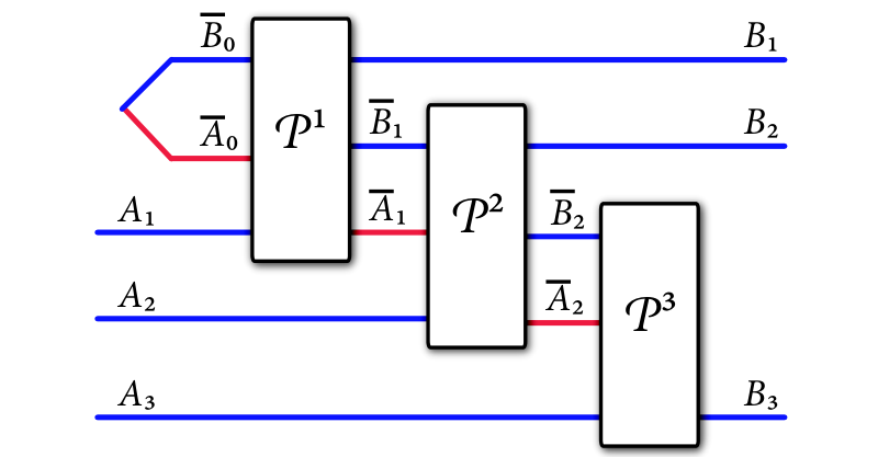
Refer to caption
Figure 3: The channel in (161), defined as the serial composition of the completely-PPT-preserving channels in the simulation.
Refer to caption
Figure 4: The exact channel simulation condition in (156) is equivalent to the condition that the Choi operators as depicted above are equal, as written in (162).

The nn-shot exact sequential simulation cost of the channel 𝒩A→B\mathcal{N}_{A\rightarrow B} is then defined as

EPPT(𝒩A→B,n)≔inf{log2M:(𝒩A→B)⊗n(ΓRn​An)=𝒫An​A¯0​B¯0→Bn(ΓRn​An⊗ΦA¯0​B¯0M)},E_{\operatorname{PPT}}(\mathcal{N}_{A\rightarrow B},n)\coloneqq\inf\big\{\log_{2}M\mathrel{\mathop{\mathchar 58\relax}}\\ (\mathcal{N}_{A\rightarrow B})^{\otimes n}(\Gamma_{R^{n}A^{n}})=\mathcal{P}_{A^{n}\overline{A}_{0}\overline{B}_{0}\rightarrow B^{n}}(\Gamma_{R^{n}A^{n}}\otimes\Phi_{\overline{A}_{0}\overline{B}_{0}}^{M})\big\}, (163)

where the optimization is with respect to sequential protocols of the form in (155) and the channel 𝒫An​A¯0​B¯0→Bn\mathcal{P}_{A^{n}\overline{A}_{0}\overline{B}_{0}\rightarrow B^{n}} is defined as in (161). The exact (sequential) simulation cost of the channel 𝒩A→B\mathcal{N}_{A\rightarrow B} is defined as

EPPT​(𝒩A→B)≔lim supn→∞1n​EPPT​(𝒩A→B,n).E_{\operatorname{PPT}}(\mathcal{N}_{A\rightarrow B})\coloneqq\limsup_{n\rightarrow\infty}\frac{1}{n}E_{\operatorname{PPT}}(\mathcal{N}_{A\rightarrow B},n). (164)

The condition in (162) illustrates that a sequential simulation is a particular kind of parallel simulation, but with more constraints. That is, in a parallel simulation, the channel 𝒫An​A¯0​B¯0→Bn\mathcal{P}_{A^{n}\overline{A}_{0}\overline{B}_{0}\rightarrow B^{n}} can be arbitrary, whereas in a sequential simulation, it is constrained to have the form in (155). For this reason, we can immediately conclude the following bound for every integer n≥1n\geq 1:

EPPT(1)​((𝒩A→B)⊗n)≤EPPT​(𝒩A→B,n),E_{\operatorname{PPT}}^{(1)}((\mathcal{N}_{A\rightarrow B})^{\otimes n})\leq E_{\operatorname{PPT}}(\mathcal{N}_{A\rightarrow B},n), (165)

which in turn implies that

EPPT(p)​(𝒩A→B)≤EPPT​(𝒩A→B).E_{\operatorname{PPT}}^{(p)}(\mathcal{N}_{A\rightarrow B})\leq E_{\operatorname{PPT}}(\mathcal{N}_{A\rightarrow B}). (166)

IV.3 Physical justification for definition of exact sequential channel simulation

The most general method for distinguishing the nn channel uses from its simulation is with an adaptive discrimination strategy. Such a strategy was described in Wil 18 and consists of an initial state ρR1​A1\rho_{R_{1}A_{1}}, a set {𝒜Ri​Bi→Ri+1​Ai+1(i)}i=1n−1\{\mathcal{A}_{R_{i}B_{i}\rightarrow R_{i+1}A_{i+1}}^{(i)}\}_{i=1}^{n-1} of adaptive channels, and a quantum measurement {QRn​Bn,𝟙Rn​Bn−QRn​Bn}\{Q_{R_{n}B_{n}},{\mathds{1}}_{R_{n}B_{n}}-Q_{R_{n}B_{n}}\}. Let us employ the shorthand {ρ,𝒜,Q}\{\rho,\mathcal{A},Q\} to abbreviate such a discrimination strategy. Note that, in performing a discrimination strategy, the discriminator has a full description of the channel 𝒩A→B\mathcal{N}_{A\rightarrow B} and the simulation protocol, which consists of ΦA¯0​B¯0\Phi_{\overline{A}_{0}\overline{B}_{0}} and the set in (155). If this discrimination strategy is performed on the nn uses of the actual channel 𝒩A→B\mathcal{N}_{A\rightarrow B}, the relevant states involved are

ρRi+1​Ai+1≔𝒜Ri​Bi→Ri+1​Ai+1(i)​(ρRi​Bi),\rho_{R_{i+1}A_{i+1}}\coloneqq\mathcal{A}_{R_{i}B_{i}\rightarrow R_{i+1}A_{i+1}}^{(i)}(\rho_{R_{i}B_{i}}), (167)

for i∈{1,…,n−1}i\in\left\{1,\ldots,n-1\right\} and

ρRi​Bi≔𝒩Ai→Bi​(ρRi​Ai),\rho_{R_{i}B_{i}}\coloneqq\mathcal{N}_{A_{i}\rightarrow B_{i}}(\rho_{R_{i}A_{i}}), (168)

for i∈{1,…,n}i\in\left\{1,\ldots,n\right\}. If this discrimination strategy is performed on the simulation protocol discussed above, then the relevant states involved are

τR1​B1​A¯1​B¯1\displaystyle\tau_{R_{1}B_{1}\overline{A}_{1}\overline{B}_{1}} ≔𝒫A1​A¯0​B¯0→B1​A¯1​B¯1(1)​(τR1​A1⊗ΦA¯0​B¯0),\displaystyle\coloneqq\mathcal{P}_{A_{1}\overline{A}_{0}\overline{B}_{0}\rightarrow B_{1}\overline{A}_{1}\overline{B}_{1}}^{(1)}(\tau_{R_{1}A_{1}}\otimes\Phi_{\overline{A}_{0}\overline{B}_{0}}),
τRi+1​Ai+1​A¯i​B¯i\displaystyle\tau_{R_{i+1}A_{i+1}\overline{A}_{i}\overline{B}_{i}} ≔𝒜Ri​Bi→Ri+1​Ai+1(i)​(τRi​Bi​A¯i​B¯i),\displaystyle\coloneqq\mathcal{A}_{R_{i}B_{i}\rightarrow R_{i+1}A_{i+1}}^{(i)}(\tau_{R_{i}B_{i}\overline{A}_{i}\overline{B}_{i}}), (169)

for i∈{1,…,n−1}i\in\left\{1,\ldots,n-1\right\}, where τR1​A1=ρR1​A1\tau_{R_{1}A_{1}}=\rho_{R_{1}A_{1}}, and

τRi​Bi​A¯i​B¯i≔𝒫Ai​A¯i−1​B¯i−1→Bi​A¯i​B¯i(i)​(τRi​Ai​A¯i−1​B¯i−1),\tau_{R_{i}B_{i}\overline{A}_{i}\overline{B}_{i}}\coloneqq\mathcal{P}_{A_{i}\overline{A}_{i-1}\overline{B}_{i-1}\rightarrow B_{i}\overline{A}_{i}\overline{B}_{i}}^{(i)}(\tau_{R_{i}A_{i}\overline{A}_{i-1}\overline{B}_{i-1}}), (170)

for i∈{2,…,n}i\in\left\{2,\ldots,n\right\}. The discriminator then performs the measurement {QRn​Bn,𝟙Rn​Bn−QRn​Bn}\{Q_{R_{n}B_{n}},{\mathds{1}}_{R_{n}B_{n}}-Q_{R_{n}B_{n}}\} and guesses “actual channel” if the outcome is QRn​BnQ_{R_{n}B_{n}} and “simulation” if the outcome is 𝟙Rn​Bn−QRn​Bn{\mathds{1}}_{R_{n}B_{n}}-Q_{R_{n}B_{n}}. Figure 5 depicts the discrimination strategy in the case that the actual channel is called n=3n=3 times and in the case that the simulation is performed.

Refer to caption
Figure 5: An adaptive protocol for discriminating the original channels (top) from their simulation (bottom).

From the physical point of view, the nn channel uses of 𝒩A→B\mathcal{N}_{A\rightarrow B} are perfectly indistinguishable from the simulation if every possible discrimination strategy as described above leads to the exact same final decision probabilities. That is, for all possible discrimination strategies, the original channels and their simulation are indistinguishable if the following equality holds

Tr⁡QRn​Bn​ρRn​Bn=Tr⁡QRn​Bn​τRn​Bn.\operatorname{Tr}Q_{R_{n}B_{n}}\rho_{R_{n}B_{n}}=\operatorname{Tr}Q_{R_{n}B_{n}}\tau_{R_{n}B_{n}}. (171)

We now prove that this physical notion of exact channel simulation is equivalent to the more mathematical notion of exact channel simulation described in the previous section. First, suppose that the physical notion of exact channel simulation holds; i.e., the equality in (171) holds for all possible discrimination strategies. Then this means that ρRn​Bn=τRn​Bn\rho_{R_{n}B_{n}}=\tau_{R_{n}B_{n}} for all possible discrimination strategies. One possible strategy could be to pick the input state for each system AiA_{i} as one of the following states

ρAx,y={|x⟩​⟨x|Aif ​x=y12​(|x⟩A+|y⟩A)​(⟨x|A+⟨y|A)if ​x<y12​(|x⟩A+i​|y⟩A)​(⟨x|A−i​⟨y|A)if ​x>y.\rho_{A}^{x,y}=\left\{\begin{array}[c]{cc}|x\rangle\!\langle x|_{A}&\text{if }x=y\\ \frac{1}{2}\left(|x\rangle_{A}+|y\rangle_{A}\right)\left(\langle x|_{A}+\langle y|_{A}\right)&\text{if }x<y\\ \frac{1}{2}\left(|x\rangle_{A}+i|y\rangle_{A}\right)\left(\langle x|_{A}-i\langle y|_{A}\right)&\text{if }x>y\end{array}\right.. (172)

and the output system BiB_{i} could be measured in the same way, but with respect to an orthonormal basis for the output system. Then all input state choices and measurement outcomes could be stored in auxiliary classical registers. Consider that for all x,yx,y such that x<yx<y, the following holds

|x⟩​⟨y|A\displaystyle|x\rangle\!\langle y|_{A} =(ρAx,y−12​ρAx,x−12​ρAy,y)\displaystyle=\left(\rho_{A}^{x,y}-\frac{1}{2}\rho_{A}^{x,x}-\frac{1}{2}\rho_{A}^{y,y}\right)
−i⁡(ρAy,x−12​ρAx,x−12​ρAy,y),\displaystyle\qquad-i\left(\rho_{A}^{y,x}-\frac{1}{2}\rho_{A}^{x,x}-\frac{1}{2}\rho_{A}^{y,y}\right), (173)
|y⟩​⟨x|A\displaystyle|y\rangle\!\langle x|_{A} =(ρAx,y−12​ρAx,x−12​ρAy,y)\displaystyle=\left(\rho_{A}^{x,y}-\frac{1}{2}\rho_{A}^{x,x}-\frac{1}{2}\rho_{A}^{y,y}\right)
+i⁡(ρAy,x−12​ρAx,x−12​ρAy,y),\displaystyle\qquad+i\left(\rho_{A}^{y,x}-\frac{1}{2}\rho_{A}^{x,x}-\frac{1}{2}\rho_{A}^{y,y}\right), (174)

so that linear combinations of all the outcomes realize the operator basis discussed in the mathematical definition of equivalence. Since the equivalence holds for all possible discrimination strategies, we can collect the data from them in the auxiliary registers, and then finally conclude that the condition in (156) holds.

Refer to caption
Figure 6: The discrimination strategy ρR1​A1\rho_{R_{1}A_{1}} and {𝒜Ri​Bi→Ri+1​Ai+1(i)}i=1n−1\{\mathcal{A}_{R_{i}B_{i}\rightarrow R_{i+1}A_{i+1}}^{(i)}\}_{i=1}^{n-1} represented as a single channel 𝒜Bn→An​Rn\mathcal{A}_{B^{n}\rightarrow A^{n}R_{n}}, as written in (175).

To see that the mathematical notion of exact sequential simulation implies the physical one, we use the method of post-selected teleportation, essentially the same idea as what was used in the proof of (BSW 11, Theorem 4). Consider the channel defined by the serial composition of the channels in the discrimination strategy {ρ,𝒜,Q}\{\rho,\mathcal{A},Q\}:

𝒜Bn→An​Rn=𝒜Rn−1​Bn−1→Rn​An(n−1)∘⋯∘𝒜R2​B2→R3​A3(2)∘𝒜R1​B1→R2​A2(1)∘ρR1​A1,\mathcal{A}_{B^{n}\rightarrow A^{n}R_{n}}=\mathcal{A}_{R_{n-1}B_{n-1}\rightarrow R_{n}A_{n}}^{(n-1)}\circ\cdots\circ\\ \mathcal{A}_{R_{2}B_{2}\rightarrow R_{3}A_{3}}^{(2)}\circ\mathcal{A}_{R_{1}B_{1}\rightarrow R_{2}A_{2}}^{(1)}\circ\rho_{R_{1}A_{1}}, (175)

where the notation ρR1​A1\rho_{R_{1}A_{1}} indicates a preparation channel that tensors in the state ρR1​A1\rho_{R_{1}A_{1}}. Figure 6 depicts this channel. By acting on both sides of the exact simulation condition with the channel and then the projection onto |Γ⟩​⟨Γ|An​Sn|\Gamma\rangle\!\langle\Gamma|_{A^{n}S^{n}}, with S≃RS\simeq R, we find that

⟨Γ|An​Sn​[𝒜Bn→An​Rn∘(𝒩A→B)⊗n​(ΓSn​An)]|Γ⟩An​Sn=⟨Γ|An​Sn​[𝒜Bn→An​Rn∘𝒫An​A¯0​B¯0→Bn​(ΓSn​An⊗ΦA¯0​B¯0M)]|Γ⟩An​Sn.\langle\Gamma|_{A^{n}S^{n}}\left[\mathcal{A}_{B^{n}\rightarrow A^{n}R_{n}}\circ(\mathcal{N}_{A\rightarrow B})^{\otimes n}(\Gamma_{S^{n}A^{n}})\right]|\Gamma\rangle_{A^{n}S^{n}}\\ =\langle\Gamma|_{A^{n}S^{n}}\left[\mathcal{A}_{B^{n}\rightarrow A^{n}R_{n}}\circ\mathcal{P}_{A^{n}\overline{A}_{0}\overline{B}_{0}\rightarrow B^{n}}(\Gamma_{S^{n}A^{n}}\otimes\Phi_{\overline{A}_{0}\overline{B}_{0}}^{M})\right]|\Gamma\rangle_{A^{n}S^{n}}. (176)

where

|Γ⟩An​Sn=|Γ⟩A1​S1⊗|Γ⟩A2​S2⊗⋯⊗|Γ⟩An​Sn.|\Gamma\rangle_{A^{n}S^{n}}=|\Gamma\rangle_{A_{1}S_{1}}\otimes|\Gamma\rangle_{A_{2}S_{2}}\otimes\cdots\otimes|\Gamma\rangle_{A_{n}S_{n}}. (177)

From the method of post-selected teleportation, we conclude that

⟨Γ|An​Sn​[𝒜Bn→An​Rn∘(𝒩A→B)⊗n​(ΓSn​An)]|Γ⟩An​Sn\displaystyle\langle\Gamma|_{A^{n}S^{n}}\left[\mathcal{A}_{B^{n}\rightarrow A^{n}R_{n}}\circ(\mathcal{N}_{A\rightarrow B})^{\otimes n}(\Gamma_{S^{n}A^{n}})\right]|\Gamma\rangle_{A^{n}S^{n}} =ρRn​Bn,\displaystyle=\rho_{R_{n}B_{n}}, (178)
⟨Γ|An​Sn​[𝒜Bn→An​Rn∘𝒫An​A¯0​B¯0→Bn​(ΓSn​An⊗ΦA¯0​B¯0M)]|Γ⟩An​Sn\displaystyle\langle\Gamma|_{A^{n}S^{n}}\left[\mathcal{A}_{B^{n}\rightarrow A^{n}R_{n}}\circ\mathcal{P}_{A^{n}\overline{A}_{0}\overline{B}_{0}\rightarrow B^{n}}(\Gamma_{S^{n}A^{n}}\otimes\Phi_{\overline{A}_{0}\overline{B}_{0}}^{M})\right]|\Gamma\rangle_{A^{n}S^{n}} =τRn​Bn.\displaystyle=\tau_{R_{n}B_{n}}. (179)

Putting these together, we finally conclude that

ρRn​Bn=τRn​Bn.\rho_{R_{n}B_{n}}=\tau_{R_{n}B_{n}}. (180)

Thus, no physical discrimination strategy can distinguish the original channels from their simulation if the exact simulation condition in (162) holds. Figure 7 depicts the operator 𝒜Bn→An​Rn∘𝒫An​A¯0​B¯0→Bn​(ΓSn​An⊗ΦA¯0​B¯0M)\mathcal{A}_{B^{n}\rightarrow A^{n}R_{n}}\circ\mathcal{P}_{A^{n}\overline{A}_{0}\overline{B}_{0}\rightarrow B^{n}}(\Gamma_{S^{n}A^{n}}\otimes\Phi_{\overline{A}_{0}\overline{B}_{0}}^{M}) in order to help visualize the above argument.

Refer to caption
Figure 7: This figure depicts the operator 𝒜Bn→An​Rn∘𝒫An​A¯0​B¯0→Bn​(ΓSn​An⊗ΦA¯0​B¯0M)\mathcal{A}_{B^{n}\rightarrow A^{n}R_{n}}\circ\mathcal{P}_{A^{n}\overline{A}_{0}\overline{B}_{0}\rightarrow B^{n}}(\Gamma_{S^{n}A^{n}}\otimes\Phi_{\overline{A}_{0}\overline{B}_{0}}^{M}) in order to help visualize the argument in (176)–(180). By projecting the systems S1​A1S_{1}A_{1} onto ⟨Γ|S1​A1\langle\Gamma|_{S_{1}A_{1}}, S2​A2S_{2}A_{2} onto ⟨Γ|S2​A2\langle\Gamma|_{S_{2}A_{2}}, and S3​A3S_{3}A_{3} onto ⟨Γ|S3​A3\langle\Gamma|_{S_{3}A_{3}}, the method of post-selected teleportation guarantees that the remaining state is τR3​B3\tau_{R_{3}B_{3}}, which is the final state of the bottom part of Figure 5.

IV.4 Exact sequential channel simulation cost

We first establish the following bounds on the nn-shot exact sequential simulation cost:

Proposition 18

Let 𝒩A→B\mathcal{N}_{A\rightarrow B} be a quantum channel such that Eκ​(𝒩)>0E_{\kappa}(\mathcal{N})>0. Then the nn-shot exact sequential simulation cost is bounded as

log2⁡[2n​Eκ​(𝒩)−1]\displaystyle\log_{2}\left[2^{nE_{\kappa}(\mathcal{N})}-1\right] ≤EPPT​(𝒩A→B,n)\displaystyle\leq E_{\operatorname{PPT}}(\mathcal{N}_{A\rightarrow B},n) (181)
≤log2⁡[2(n+1)​Eκ​(𝒩)−12Eκ​(𝒩)−1].\displaystyle\leq\log_{2}\left[\frac{2^{\left(n+1\right)E_{\kappa}(\mathcal{N})}-1}{2^{E_{\kappa}(\mathcal{N})}-1}\right]. (182)

If Eκ​(𝒩)=0E_{\kappa}(\mathcal{N})=0, then EPPT​(𝒩A→B,n)=0E_{\operatorname{PPT}}(\mathcal{N}_{A\rightarrow B},n)=0.

Proof.  Suppose that Eκ​(𝒩)>0E_{\kappa}(\mathcal{N})>0. The inequality

log2⁡[2n​Eκ​(𝒩)−1]≤EPPT​(𝒩A→B,n)\log_{2}\left[2^{nE_{\kappa}(\mathcal{N})}-1\right]\leq E_{\operatorname{PPT}}(\mathcal{N}_{A\rightarrow B},n) (183)

is a direct consequence of (165), Proposition 16, and Proposition 11.

So we now prove the other inequality. The main idea behind the construction is for the iith completely-PPT-preserving channel to perform the following exact simulation:

𝒫Ai​A¯i−1​B¯i−1→Bi​A¯i​B¯i(i)​(ρAi⊗ΦA¯i−1​B¯i−1Mi−1)=𝒩A→B​(ρAi)⊗ΦA¯i​B¯iMi,\mathcal{P}_{A_{i}\overline{A}_{i-1}\overline{B}_{i-1}\rightarrow B_{i}\overline{A}_{i}\overline{B}_{i}}^{(i)}(\rho_{A_{i}}\otimes\Phi_{\overline{A}_{i-1}\overline{B}_{i-1}}^{M_{i-1}})=\\ \mathcal{N}_{A\rightarrow B}(\rho_{A_{i}})\otimes\Phi_{\overline{A}_{i}\overline{B}_{i}}^{M_{i}}, (184)

for i∈{1,…,n−1}i\in\left\{1,\ldots,n-1\right\} and for the nnth completely-PPT-preserving channel to perform the following exact simulation:

𝒫An​A¯n−1​B¯n−1→Bn(n)​(ρAn⊗ΦA¯n−1​B¯n−1Mn−1)=𝒩A→B​(ρAn).\mathcal{P}_{A_{n}\overline{A}_{n-1}\overline{B}_{n-1}\rightarrow B_{n}}^{(n)}(\rho_{A_{n}}\otimes\Phi_{\overline{A}_{n-1}\overline{B}_{n-1}}^{M_{n-1}})=\mathcal{N}_{A\rightarrow B}(\rho_{A_{n}}). (185)

Note that, in order to perform the simulation in (184), we could actually simulate the channel 𝒩A→B⊗idMi\mathcal{N}_{A\rightarrow B}\otimes\operatorname{id}^{M_{i}}, and then send one share of the maximally entangled state ΦA¯i​B¯iMi\Phi_{\overline{A}_{i}\overline{B}_{i}}^{M_{i}} through the exactly simulated identity channel idMi\operatorname{id}^{M_{i}} to produce the output in (184).

Thus, we should now determine an upper bound on the simulation cost when using this construction. The most effective way to do so is to start from the final (nnth) simulation. By the one-shot bound from Proposition 16, its cost log2⁡Mn−1\log_{2}M_{n-1} is bounded as

log2⁡Mn−1≤log2⁡[2Eκ​(𝒩)+1].\log_{2}M_{n-1}\leq\log_{2}\left[2^{E_{\kappa}(\mathcal{N})}+1\right]. (186)

The cost log2⁡Mn−2\log_{2}M_{n-2} of the n−1n-1 simulation is then bounded as

log2⁡Mn−2\displaystyle\log_{2}M_{n-2} ≤log2⁡[2Eκ​(𝒩⊗idMn−1)+1]\displaystyle\leq\log_{2}\left[2^{E_{\kappa}(\mathcal{N}\otimes\operatorname{id}^{M_{n-1}})}+1\right] (187)
≤log2⁡[2Eκ​(𝒩)+log2⁡Mn−1+1]\displaystyle\leq\log_{2}\left[2^{E_{\kappa}(\mathcal{N})+\log_{2}M_{n-1}}+1\right] (188)
=log2⁡[2Eκ​(𝒩)​Mn−1+1]\displaystyle=\log_{2}\left[2^{E_{\kappa}(\mathcal{N})}M_{n-1}+1\right] (189)
≤log2⁡[2Eκ​(𝒩)​(2Eκ​(𝒩)+1)+1]\displaystyle\leq\log_{2}\left[2^{E_{\kappa}(\mathcal{N})}\left(2^{E_{\kappa}(\mathcal{N})}+1\right)+1\right] (190)
=log2⁡[∑ℓ=022ℓ​Eκ​(𝒩)],\displaystyle=\log_{2}\left[\sum_{\ell=0}^{2}2^{\ell E_{\kappa}(\mathcal{N})}\right], (191)

where we made use of the subadditivity inequality from Proposition 11. Performing this kind of reasoning iteratively, going backward until the first simulation, we find the following bound:

log2⁡M0≤log2⁡[∑ℓ=0n2ℓ​Eκ​(𝒩)]=log2⁡[2(n+1)​Eκ​(𝒩)−12Eκ​(𝒩)−1].\log_{2}M_{0}\leq\log_{2}\left[\sum_{\ell=0}^{n}2^{\ell E_{\kappa}(\mathcal{N})}\right]=\log_{2}\left[\frac{2^{\left(n+1\right)E_{\kappa}(\mathcal{N})}-1}{2^{E_{\kappa}(\mathcal{N})}-1}\right]. (192)

If Eκ​(𝒩)=0E_{\kappa}(\mathcal{N})=0, then the channel 𝒩\mathcal{N} is PPT entanglement binding by Proposition 13 and thus can be simulated at no cost, so that EPPT​(𝒩A→B,n)=0E_{\operatorname{PPT}}(\mathcal{N}_{A\rightarrow B},n)=0. This concludes the proof. ■\blacksquare

Theorem 19 (Exact sequential cost)

Let 𝒩A→B\mathcal{N}_{A\rightarrow B} be a quantum channel. Then the exact sequential channel simulation cost of 𝒩A→B\mathcal{N}_{A\rightarrow B} is equal to its κ\kappa-entanglement:

EPPT​(𝒩A→B)=Eκ​(𝒩A→B).E_{\operatorname{PPT}}(\mathcal{N}_{A\rightarrow B})=E_{\kappa}(\mathcal{N}_{A\rightarrow B}). (193)

Proof.  First suppose that Eκ​(𝒩)>0E_{\kappa}(\mathcal{N})>0. The lower bound follows from Proposition 18 and Theorem 17. The upper bound follows from Proposition 18:

lim supn→∞1n​EPPT​(𝒩A→B,n)\displaystyle\limsup_{n\rightarrow\infty}\frac{1}{n}E_{\operatorname{PPT}}(\mathcal{N}_{A\rightarrow B},n)
≤lim supn→∞1n​log2​[2(n+1)​Eκ​(𝒩)−12Eκ​(𝒩)−1]\displaystyle\leq\limsup_{n\rightarrow\infty}\frac{1}{n}\log_{2}\left[\frac{2^{\left(n+1\right)E_{\kappa}(\mathcal{N})}-1}{2^{E_{\kappa}(\mathcal{N})}-1}\right] (194)
=lim supn→∞1n​log2​[2n​Eκ​(𝒩)−2−Eκ​(𝒩)1−2−Eκ​(𝒩)]\displaystyle=\limsup_{n\rightarrow\infty}\frac{1}{n}\log_{2}\left[\frac{2^{nE_{\kappa}(\mathcal{N})}-2^{-E_{\kappa}(\mathcal{N})}}{1-2^{-E_{\kappa}(\mathcal{N})}}\right] (195)
=Eκ​(𝒩).\displaystyle=E_{\kappa}(\mathcal{N}). (196)

If Eκ​(𝒩)=0E_{\kappa}(\mathcal{N})=0, then the channel 𝒩\mathcal{N} is PPT entanglement binding by Proposition 13 and thus can be simulated at no cost. This concludes the proof. ■\blacksquare

By combining Theorems 17 and 19, we reach the conclusion that the exact entanglement cost of parallel and sequential simulation of quantum channels are in fact equal and given by the κ\kappa-entanglement of the channel. Thus, the κ\kappa-entanglement is a fundamental measure of the entanglement of a quantum channel. Not only is it efficiently computable by means of a semi-definite program (for finite-dimensional channels), but it also possesses a direct operational meaning in terms of these channel simulation tasks. It is the only known channel entanglement measure possessing these properties, and from this perspective, it can be helpful in understanding the fundamental structure of entanglement of quantum channels.

IV.5 PPT-simulable channels

Although the theory of exact simulation of quantum channels under PPT operations simplifies significantly due to Theorems 17 and 19, there is a class of channels for which the theory is even simpler. These channels were defined in KW 18 and are known as PPT-simulable channels. In this section, we recall their definition and show how the theory of exact entanglement cost is quite simple for certain PPT-simulable channels.

Definition 4 (PPT-simulable channel KW 18)

A channel 𝒩A→B\mathcal{N}_{A\rightarrow B} is PPT-simulable with associated resource state ωA′​B′\omega_{A^{\prime}B^{\prime}} if there exists a completely PPT-preserving channel 𝒫A​A′​B′→B\mathcal{P}_{AA^{\prime}B^{\prime}\rightarrow B} such that, for every input state ρA\rho_{A}

𝒩A→B​(ρA)=𝒫A​A′​B′→B​(ρA⊗ωA′​B′).\mathcal{N}_{A\rightarrow B}(\rho_{A})=\mathcal{P}_{AA^{\prime}B^{\prime}\rightarrow B}(\rho_{A}\otimes\omega_{A^{\prime}B^{\prime}}). (197)

A particular kind of PPT-simulable channel is one that is resource-seizable, as defined in (Wil 18, Section VI):

Definition 5 (Resource-seizable Wil 18)

Let 𝒩A→B\mathcal{N}_{A\rightarrow B} be a PPT-simulable channel with associated resource state ωA′​B′\omega_{A^{\prime}B^{\prime}}. The channel 𝒩A→B\mathcal{N}_{A\rightarrow B} is resource-seizable if there exists a PPT state τAM​A​BM\tau_{A_{M}AB_{M}} and a completely PPT-preserving post-processing channel 𝒟AM​B​BM→A′​B′\mathcal{D}_{A_{M}BB_{M}\rightarrow A^{\prime}B^{\prime}} such that

𝒟AM​B​BM→A′​B′​(𝒩A→B​(τAM​A​BM))=ωA′​B′.\mathcal{D}_{A_{M}BB_{M}\rightarrow A^{\prime}B^{\prime}}(\mathcal{N}_{A\rightarrow B}(\tau_{A_{M}AB_{M}}))=\omega_{A^{\prime}B^{\prime}}. (198)

For PPT-simulable channels, it follows that the exact entanglement cost of sequential channel simulation is bounded from above by the exact entanglement cost of the underlying resource state:

Theorem 20

Let 𝒩A→B\mathcal{N}_{A\rightarrow B} be a PPT-simulable channel with associated resource state ωA′​B′\omega_{A^{\prime}B^{\prime}}. Then the PPT-assisted entanglement cost of a channel is bounded from above as

EPPT​(𝒩A→B)≤EPPT​(ωA′​B′)=Eκ​(ωA′​B′).E_{\operatorname{PPT}}(\mathcal{N}_{A\rightarrow B})\leq E_{\operatorname{PPT}}(\omega_{A^{\prime}B^{\prime}})=E_{\kappa}(\omega_{A^{\prime}B^{\prime}}). (199)

Proof.  The proof for this inequality follows the same reasoning given in (Wil 18, Corollary 1). First simulate a large number of copies of the resource state ωA′​B′\omega_{A^{\prime}B^{\prime}} and then use the PPT-preserving channel 𝒫A​A′​B′→B\mathcal{P}_{AA^{\prime}B^{\prime}\rightarrow B} from (197) to simulate the channel 𝒩A→B\mathcal{N}_{A\rightarrow B}. The equality follows from Proposition 6. ■\blacksquare

If a PPT-simulable channel is additionally resource-seizable, then its exact entanglement cost is given by the κ\kappa-entanglement of the underlying resource state:

Theorem 21

Let 𝒩A→B\mathcal{N}_{A\rightarrow B} be a PPT-simulable channel with associated resource state ωA′​B′\omega_{A^{\prime}B^{\prime}}. Suppose furthermore that it is resource-seizable, as given in Definition 5. Then

EPPT​(𝒩A→B)\displaystyle E_{\operatorname{PPT}}(\mathcal{N}_{A\rightarrow B}) =EPPT(p)​(𝒩A→B)=Eκ​(𝒩A→B)\displaystyle=E_{\operatorname{PPT}}^{(p)}(\mathcal{N}_{A\rightarrow B})=E_{\kappa}(\mathcal{N}_{A\rightarrow B}) (200)
=EPPT​(ωA′​B′)=Eκ​(ωA′​B′).\displaystyle=E_{\operatorname{PPT}}(\omega_{A^{\prime}B^{\prime}})=E_{\kappa}(\omega_{A^{\prime}B^{\prime}}). (201)

Proof.  The following inequality

EPPT​(𝒩A→B)≤EPPT​(ωA′​B′)=Eκ​(ωA′​B′).E_{\operatorname{PPT}}(\mathcal{N}_{A\rightarrow B})\leq E_{\operatorname{PPT}}(\omega_{A^{\prime}B^{\prime}})=E_{\kappa}(\omega_{A^{\prime}B^{\prime}}). (202)

is a consequence of Theorem 20. To establish the opposite inequality, consider that we always have that

EPPT​(𝒩A→B)≥EPPT(p)​(𝒩A→B),E_{\operatorname{PPT}}(\mathcal{N}_{A\rightarrow B})\geq E_{\operatorname{PPT}}^{(p)}(\mathcal{N}_{A\rightarrow B}), (203)

where EPPT(p)E_{\operatorname{PPT}}^{(p)} denotes the exact parallel simulation entanglement cost. From Theorem 17, we have that

EPPT(p)​(𝒩A→B)=Eκ​(𝒩A→B).E_{\operatorname{PPT}}^{(p)}(\mathcal{N}_{A\rightarrow B})=E_{\kappa}(\mathcal{N}_{A\rightarrow B}). (204)

So it suffices to prove that

Eκ​(𝒩A→B)=Eκ​(ωA′​B′).E_{\kappa}(\mathcal{N}_{A\rightarrow B})=E_{\kappa}(\omega_{A^{\prime}B^{\prime}}). (205)

Letting ρR​A\rho_{RA} be an arbitrary input state, we have that

Eκ​(𝒩A→B​(ρR​A))\displaystyle E_{\kappa}(\mathcal{N}_{A\rightarrow B}(\rho_{RA})) =Eκ​(𝒫A​A′​B′→B​(ρR​A⊗ωA′​B′))\displaystyle=E_{\kappa}(\mathcal{P}_{AA^{\prime}B^{\prime}\rightarrow B}(\rho_{RA}\otimes\omega_{A^{\prime}B^{\prime}})) (206)
≤Eκ​(ρR​A⊗ωA′​B′)\displaystyle\leq E_{\kappa}(\rho_{RA}\otimes\omega_{A^{\prime}B^{\prime}}) (207)
=Eκ​(ωA′​B′),\displaystyle=E_{\kappa}(\omega_{A^{\prime}B^{\prime}}), (208)

where the inequality follows from the monotonicity of EκE_{\kappa} under PPT-preserving channels and the final equality follows because the bipartite cut is taken as R​A​A′|B′RAA^{\prime}|B^{\prime}. Since this holds for an arbitrary input state ρR​A\rho_{RA}, we conclude that

Eκ​(ωA′​B′)≥Eκ​(𝒩A→B).E_{\kappa}(\omega_{A^{\prime}B^{\prime}})\geq E_{\kappa}(\mathcal{N}_{A\rightarrow B}). (209)

Now we prove the opposite inequality, by using the fact that 𝒩A→B\mathcal{N}_{A\rightarrow B} is resource-seizable. Let τAM​A​BM\tau_{A_{M}AB_{M}} be the input PPT state from Definition 5. Consider that

Eκ​(ωA′​B′)\displaystyle E_{\kappa}(\omega_{A^{\prime}B^{\prime}}) =Eκ​(𝒟AM​B​BM→A′​B′​(𝒩A→B​(τAM​A​BM)))\displaystyle=E_{\kappa}(\mathcal{D}_{A_{M}BB_{M}\rightarrow A^{\prime}B^{\prime}}(\mathcal{N}_{A\rightarrow B}(\tau_{A_{M}AB_{M}}))) (210)
≤Eκ​(𝒩A→B​(τAM​A​BM))\displaystyle\leq E_{\kappa}(\mathcal{N}_{A\rightarrow B}(\tau_{A_{M}AB_{M}})) (211)
=Eκ​(𝒩A→B​(τAM​A​BM))−Eκ​(τAM​A​BM)\displaystyle=E_{\kappa}(\mathcal{N}_{A\rightarrow B}(\tau_{A_{M}AB_{M}}))-E_{\kappa}(\tau_{A_{M}AB_{M}}) (212)
≤Eκ​(𝒩A→B).\displaystyle\leq E_{\kappa}(\mathcal{N}_{A\rightarrow B}). (213)

The first inequality follows because EκE_{\kappa} does not increase under the action of the completely PPT-preserving channel 𝒟AM​B​BM→A′​B′\mathcal{D}_{A_{M}BB_{M}\rightarrow A^{\prime}B^{\prime}} (Theorem 1). The second equality follows because τAM​A​BM\tau_{A_{M}AB_{M}} is a PPT state, so that Eκ​(τAM​A​BM)=0E_{\kappa}(\tau_{A_{M}AB_{M}})=0. The final inequality is a consequence of the amortization inequality in Proposition 8. ■\blacksquare

IV.6 Relationship to other quantities

A previously known efficiently computable upper bound for quantum capacity is the partial transposition bound HW 01:

QΘ​(𝒩)≔log2⁡‖TB→B∘𝒩A→B‖◇,\displaystyle Q_{\Theta}({\cal N})\coloneqq\log_{2}\left\|T_{B\to B}\circ{\cal N}_{A\to B}\right\|_{\Diamond}, (214)

where TB→BT_{B\to B} is the transpose map and ∥⋅∥◇\|\cdot\|_{\Diamond} is the completely bounded trace norm or diamond norm. Note that ∥⋅∥◇\|\cdot\|_{\Diamond} for finite-dimensional channels is efficiently computable via semidefinite programming Wat 13.

Proposition 22

For every quantum channel 𝒩A→B{\cal N}_{A\to B}, we have that

QΘ​(𝒩A→B)≤Eκ​(𝒩A→B).\displaystyle Q_{\Theta}({\cal N}_{A\to B})\leq E_{\kappa}({\cal N}_{A\to B}). (215)

Proof.  Given an arbitrary quantum channel 𝒩A→B{\cal N}_{A\to B}, it holds that

Eκ​(𝒩A→B)\displaystyle E_{\kappa}({\cal N}_{A\to B}) =supϕR​AEκ​(𝒩A→B​(ϕR​A))\displaystyle=\sup_{\phi_{RA}}E_{\kappa}({\cal N}_{A\to B}(\phi_{RA})) (216)
≥supϕR​AEN​(𝒩A→B​(ϕR​A))\displaystyle\geq\sup_{\phi_{RA}}E_{N}({\cal N}_{A\to B}(\phi_{RA})) (217)
=supϕR​Alog2⁡‖𝒩A→B​(ϕR​A)TB‖1\displaystyle=\sup_{\phi_{RA}}\log_{2}\|{\cal N}_{A\to B}(\phi_{RA})^{T_{B}}\|_{1} (218)
=log2⁡‖TB→B∘𝒩A→B‖◇.\displaystyle=\log_{2}\left\|T_{B\to B}\circ{\cal N}_{A\to B}\right\|_{\Diamond}. (219)

The equality in (216) follows from Proposition 7. The inequality in (217) follows from the property of EκE_{\kappa} in Eq. (12). The last equality follows due to the definition of the completely bounded trace norm. ■\blacksquare

Remark 2

For qubit-input qubit-output channels, we have that

Eκ​(𝒩A→B)=QΘ​(𝒩A→B).E_{\kappa}({\cal N}_{A\to B})=Q_{\Theta}({\cal N}_{A\to B}). (220)

This follows because it suffices to optimize Eκ​(𝒩A→B)E_{\kappa}({\cal N}_{A\to B}) with respect to two-qubit input states ϕR​A\phi_{RA}, and then the output state consists of two qubits, so that the result of Ish 04 applies. That is, for this case,

Eκ​(𝒩A→B)\displaystyle E_{\kappa}({\cal N}_{A\to B}) =supϕR​AEκ​(𝒩A→B​(ϕR​A))\displaystyle=\sup_{\phi_{RA}}E_{\kappa}({\cal N}_{A\to B}(\phi_{RA})) (221)
=supϕR​AEN​(𝒩A→B​(ϕR​A))\displaystyle=\sup_{\phi_{RA}}E_{N}({\cal N}_{A\to B}(\phi_{RA})) (222)
=QΘ​(𝒩A→B).\displaystyle=Q_{\Theta}({\cal N}_{A\to B}). (223)

V Exact entanglement cost of fundamental channels

Theorem 21 provides a formula for the exact PPT-entanglement cost of an arbitrary resource-seizable, PPT-simulable channel, given in terms of the entanglement cost of the underlying resource state ωA′​B′\omega_{A^{\prime}B^{\prime}}. We detail some simple examples here for which this simplified formula applies. We also consider amplitude damping channels, for which it is necessary to invoke Theorems 17 and 19 in order to determine their exact entanglement costs.

Let us begin by recalling the notion of a covariant channel 𝒩A→B\mathcal{N}_{A\rightarrow B} Hol 02. For a group GG with unitary channel representations {𝒰Ag}g∈G\{\mathcal{U}_{A}^{g}\}_{g\in G} and {𝒱Bg}g∈G\{\mathcal{V}_{B}^{g}\}_{g\in G} acting on the input system AA and output system BB of the channel 𝒩A→B\mathcal{N}_{A\rightarrow B}, the channel 𝒩A→B\mathcal{N}_{A\rightarrow B} is covariant with respect to the groupG~G if the following equality holds for all g∈Gg\in G:

𝒩A→B∘𝒰Ag=𝒱Bg∘𝒩A→B.\mathcal{N}_{A\rightarrow B}\circ\mathcal{U}_{A}^{g}=\mathcal{V}_{B}^{g}\circ\mathcal{N}_{A\rightarrow B}. (224)

If the averaging channel is such that 1|G|​∑g𝒰Ag​(X)=Tr⁡[X]​I/|A|\frac{1}{\left|G\right|}\sum_{g}\mathcal{U}_{A}^{g}(X)=\operatorname{Tr}[X]I/\left|A\right|, then we simply say that the channel 𝒩A→B\mathcal{N}_{A\rightarrow B} is covariant.

Then from (CDP09a, Section 7), we conclude that a covariant channel is PPT-simulable with associated resource state given by the Choi state of the channel, i.e., ωA′​B′=𝒩A→B​(ΦA′​A)\omega_{A^{\prime}B^{\prime}}=\mathcal{N}_{A\rightarrow B}(\Phi_{A^{\prime}A}). As such, covariant channels are resource-seizable, so that the equality in Theorem 21 applies to all covariant channels. Thus, the exact entanglement cost of a covariant channel is equal to the exact entanglement cost of its Choi state.

V.1 Erasure channel

The quantum erasure channel is denoted by

ℰp​(ρ)=(1−p)​ρ+p⁡|e⟩​⟨e|,\displaystyle{\cal E}_{p}(\rho)=(1-p)\rho+p|e\rangle\!\langle e|, (225)

where ρ\rho is a dd-dimensional input state, p∈[0,1]p\in\left[0,1\right] is the erasure probability, and |e⟩​⟨e||e\rangle\!\langle e| is a pure erasure state orthogonal to every input state, so that the output state has d+1d+1 dimensions. This channel is covariant.

The Choi matrix of ℰp{\cal E}_{p} is given by

Jℰp=(1−p)​∑i,j=0d−1|i​i⟩​⟨j​j|+p​∑i=0d−1|i⟩​⟨i|⊗|e⟩​⟨e|.\displaystyle J_{{\cal E}_{p}}=(1-p)\sum_{i,j=0}^{d-1}|ii\rangle\!\langle jj|+p\sum_{i=0}^{d-1}|i\rangle\!\langle i|\otimes|e\rangle\!\langle e|. (226)

By direct calculation, we find that

EPPT​(ℰp)\displaystyle{E_{\operatorname{PPT}}}({\cal E}_{p}) =EPPT​(Jℰp/d)\displaystyle={E_{\operatorname{PPT}}}(J_{{\cal E}_{p}}/d) (227)
=EN​(Jℰp/d)\displaystyle=E_{N}(J_{{\cal E}_{p}}/d) (228)
=log2⁡(d⁡[1−p]+p).\displaystyle=\log_{2}(d[1-p]+p). (229)

V.2 Depolarizing channel

Consider the qudit depolarizing channel:

𝒩D,p​(ρ)=(1−p)​ρ+pd2−1​∑0≤i,j≤d−1(i,j)≠(0,0)Xi​Zj​ρ​(Xi​Zj)†,\displaystyle{\cal N}_{D,p}(\rho)=(1-p)\rho+\frac{p}{d^{2}-1}\sum_{\begin{subarray}{c}0\leq i,j\leq d-1\\ (i,j)\neq(0,0)\end{subarray}}X^{i}Z^{j}\rho(X^{i}Z^{j})^{\dagger}, (230)

where p∈[0,1]p\in[0,1] and X,ZX,Z are the generalized Pauli operators. This channel is covariant.

The Choi matrix of 𝒩D,p{\cal N}_{D,p} is

J𝒩D,p=d⁡[(1−p)​ΦA​B+pd2−1​(𝟙A​B−ΦA​B)],\displaystyle J_{{\cal N}_{D,p}}=d\left[(1-p)\Phi_{AB}+\frac{p}{d^{2}-1}({\mathds{1}}_{AB}-\Phi_{AB})\right], (231)

where Φ=1d​∑i,j=0d−1|i​i⟩​⟨j​j|\Phi=\frac{1}{d}\sum_{i,j=0}^{d-1}|ii\rangle\!\langle jj|. Observe that the state J𝒩D,pd\frac{J_{{\cal N}_{D,p}}}{d} is an isotropic state. Applying the previous result from (29), we conclude that

EPPT​(𝒩D,p)=\displaystyle{E_{\operatorname{PPT}}}({\cal N}_{D,p})= {log2⁡d⁡(1−p) if ​1−p≥1d0 if ​1−p<1d\displaystyle\begin{cases}\log_{2}d(1-p)&\text{ if }1-p\geq\frac{1}{d}\\ 0&\text{ if }1-p<\frac{1}{d}\end{cases} (232)

V.3 Dephasing channel

The qubit dephasing channel is given as

𝒟q​(ρ)=(1−q)​ρ+q​Z​ρ​Z.\mathcal{D}_{q}(\rho)=(1-q)\rho+qZ\rho Z. (233)

Note that this channel is covariant with respect to the Heisenberg–Weyl group of unitaries. The Choi matrix of 𝒟q\mathcal{D}_{q} is as follows:

J𝒟q=2​[(1−q)​ψ1+q​ψ2],\displaystyle J_{\mathcal{D}_{q}}=2[(1-q)\psi_{1}+q\psi_{2}], (234)

where

|ψ1⟩=12​(|00⟩+|11⟩),|ψ2⟩=12​(|00⟩−|11⟩).\displaystyle|\psi_{1}\rangle=\frac{1}{\sqrt{2}}(|00\rangle+|11\rangle),\quad|\psi_{2}\rangle=\frac{1}{\sqrt{2}}(|00\rangle-|11\rangle). (235)

By direct calculation, we find that

EPPT​(𝒟q)\displaystyle{E_{\operatorname{PPT}}}(\mathcal{D}_{q}) =EPPT​(J𝒟q/2)\displaystyle={E_{\operatorname{PPT}}}(J_{\mathcal{D}_{q}}/2) (236)
=EN​(J𝒟q/2)\displaystyle=E_{N}(J_{\mathcal{D}_{q}}/2) (237)
=log2⁡(1+2​|q−1/2|).\displaystyle=\log_{2}(1+2|q-1/2|). (238)

We note that this approach also works for a dd-dimensional dephasing channel.

V.4 Amplitude damping channel

An amplitude damping channel corresponds to the process of asymmetric relaxation in a quantum system, which is a key noise process in quantum information science. The qubit amplitude damping channel is given as 𝒩A​D,r=∑i=01Ei⋅Ei†{\cal N}_{AD,r}=\sum_{i=0}^{1}E_{i}\cdot E_{i}^{\dagger} with

E0=|0⟩​⟨0|+1−r|1⟩​⟨1|,E1=r​|0⟩​⟨1|,\displaystyle E_{0}=|0\rangle\!\langle 0|+\sqrt{1-r}|1\rangle\!\langle 1|,\quad E_{1}=\sqrt{r}|0\rangle\!\langle 1|, (239)

and where r∈[0,1]r\in[0,1] is the damping parameter. This channel is covariant with respect to {I,Z}\{I,Z\}, but not with respect to a one-design. So Theorem 21 does not apply, and we instead need to evaluate the exact entanglement cost of this channel by applying Theorems 17 and 19.

We plot EPPT​(𝒩A​D,r){E_{\operatorname{PPT}}}({\cal N}_{AD,r}) in Figure 8 and compare it with the max-Rains information of WD16b; WFD 19. The fact that there is a gap between these two quantities demonstrates that the resource theory of entanglement (exact PPT case) is irreversible, given that the max-Rains information is an upper bound on the exact distillable entanglement of an arbitrary channel BW 18.

Figure 8: This plot demonstrates the difference between EPPT​(𝒩A​D,r){E_{\operatorname{PPT}}}({\cal N}_{AD,r}) and Rmax​(𝒩A​D,r)R_{\max}({\cal N}_{AD,r}), where 𝒩A​D,r{\cal N}_{AD,r} is the amplitude damping channel in Section V.4. The solid line depicts EPPT​(𝒩A​D,r){E_{\operatorname{PPT}}}({\cal N}_{AD,r}) while the dashed line depicts Rmax​(𝒩A​D,r)R_{\max}({\cal N}_{AD,r}). The parameter rr ranges from 00 to 11, and the units of the rate (vertical axis) are ebits per channels use.

VI Exact entanglement cost of quantum Gaussian channels

In this subsection, we determine formulas for the exact entanglement cost of particular quantum Gaussian channels, which include all single-mode bosonic Gaussian channels with the exception of the pure-loss and pure-amplifier channels. In this sense, the results found here are complementary to those found recently in (Wil 18, Theorem 2). The presentation and background given in this section largely follows that given recently in Wil 18.

VI.1 Preliminary observations about the exact entanglement cost of single-mode bosonic Gaussian channels

The starting point for our analysis of single-mode bosonic Gaussian channels is the Holevo classification from Hol 07, in which canonical forms for all single-mode bosonic Gaussian channels have been given, classifying them up to local Gaussian unitaries acting on the input and output of the channel. It then suffices for us to focus our attention on the canonical forms, as it is self-evident from definitions that local unitaries do not alter the exact entanglement cost of a quantum channel. The thermal and amplifier channels form the class C discussed in Hol 07, and the additive-noise channels form the class B2 discussed in the same work. The classes that remain are labeled A, B1, and D in Hol 07. The channels in A and D are entanglement-breaking Hol 08, and are thus entanglement-binding, and as a consequence of Proposition 13 and Theorems 17 and 19, they have zero exact entanglement cost. Channels in the class B1 are perhaps not interesting for practical applications, and as it turns out, they have infinite quantum capacity Hol 07. Thus, their exact entanglement cost is also infinite, because a channel’s quantum capacity is a lower bound on its distillable entanglement, which is in turn a lower bound on its partial transposition bound. The partial transposition bound is finally a lower bound on its κ\kappa-entanglement, as shown in Proposition 22. For the same reason, the exact entanglement cost of the bosonic identity channel is also infinite.

VI.2 Thermal, amplifier, and additive-noise bosonic Gaussian channels

In light of the previous discussion, for the remainder of this section, let us focus our attention on the thermal, amplifier, and additive-noise channels. Each of these are defined respectively by the following Heisenberg input-output relations:

b^\displaystyle\hat{b} =η​a^+1−η​e^,\displaystyle=\sqrt{\eta}\hat{a}+\sqrt{1-\eta}\hat{e}, (240)
b^\displaystyle\hat{b} =G​a^+G−1​e^†,\displaystyle=\sqrt{G}\hat{a}+\sqrt{G-1}\hat{e}^{{\dagger}}, (241)
b^\displaystyle\hat{b} =a^+(x+i​p)/2,\displaystyle=\hat{a}+\left(x+ip\right)/\sqrt{2}, (242)

where a^\hat{a}, b^\hat{b}, and e^\hat{e} are the field-mode annihilation operators for the sender’s input, the receiver’s output, and the environment’s input of these channels, respectively.

The channel in (240) is a thermalizing channel, in which the environmental mode is prepared in a thermal state θ⁡(NB)\theta(N_{B}) of mean photon number NB≥0N_{B}\geq 0, defined as

θ⁡(NB)≔1NB+1​∑n=0∞(NBNB+1)n​|n⟩​⟨n|,\theta(N_{B})\coloneqq\frac{1}{N_{B}+1}\sum_{n=0}^{\infty}\left(\frac{N_{B}}{N_{B}+1}\right)^{n}|n\rangle\!\langle n|, (243)

where {|n⟩}n=0∞\left\{|n\rangle\right\}_{n=0}^{\infty} is the orthonormal, photonic number-state basis. When NB=0N_{B}=0, the state θ⁡(NB)\theta(N_{B}) reduces to the vacuum state, in which case the resulting channel in (240) is called the pure-loss channel—it is said to be quantum-limited in this case because the environment is injecting the minimum amount of noise allowed by quantum mechanics. The parameter η∈(0,1)\eta\in(0,1) is the transmissivity of the channel, representing the average fraction of photons making it from the input to the output of the channel. Let ℒη,NB\mathcal{L}_{\eta,N_{B}} denote this channel, and we make the further abbreviation ℒη≡ℒη,NB=0\mathcal{L}_{\eta}\equiv\mathcal{L}_{\eta,N_{B}=0} when it is the pure-loss channel. The channel in (240) is entanglement-breaking when (1−η)​NB≥η\left(1-\eta\right)N_{B}\geq\eta Hol 08, and is thus entanglement-binding in this case, and as a consequence of Proposition 13 and Theorems 17 and 19, it has zero exact entanglement cost for these values.

The channel in (241) is an amplifier channel, and the parameter G>1G>1 is its gain. For this channel, the environment is prepared in the thermal state θ⁡(NB)\theta(N_{B}). If NB=0N_{B}=0, the amplifier channel is called the pure-amplifier channel—it is said to be quantum-limited for a similar reason as stated above. Let 𝒜G,NB\mathcal{A}_{G,N_{B}} denote this channel, and we make the further abbreviation 𝒜G≡𝒜G,NB=0\mathcal{A}_{G}\equiv\mathcal{A}_{G,N_{B}=0} when it is the quantum-limited amplifier channel. The channel in (241) is entanglement-breaking when (G−1)​NB≥1\left(G-1\right)N_{B}\geq 1 Hol 08, and is thus entanglement-binding, and as a consequence of Proposition 13 and Theorems 17 and 19, it has zero exact entanglement cost for these values.

Finally, the channel in (242) is an additive-noise channel, representing a quantum generalization of the classical additive white Gaussian noise channel. In (242), xx and pp are zero-mean, independent Gaussian random variables each having variance ξ≥0\xi\geq 0. Let 𝒯ξ\mathcal{T}_{\xi} denote this channel. The channel in (242) is entanglement-breaking when ξ≥1\xi\geq 1 Hol 08, and is thus entanglement-binding, and as a consequence of Proposition 13 and Theorems 17 and 19, it has zero exact entanglement cost for these values.

Kraus representations for the channels in (240)–(242) are available in ISS 11, which can be helpful for further understanding their action on input quantum states.

Due to the entanglement-breaking regions discussed above, we are left with a limited range of single-mode bosonic Gaussian channels to consider, which is delineated by the white strip in Figure 1 of GGPCH 14.

VI.3 Exact entanglement cost of thermal, amplifier, and additive-noise bosonic Gaussian channels

We can now state our main result for this section, which applies to all thermal, amplifier, and additive-noise channels that are neither entanglement-breaking nor quantum-limited:

Theorem 23

For a thermal channel ℒη,NB\mathcal{L}_{\eta,N_{B}} with transmissivity η∈(0,1)\eta\in(0,1) and thermal photon number NB∈(0,η/[1−η])N_{B}\in(0,\eta/[1-\eta]), an amplifier channel 𝒜G,NB\mathcal{A}_{G,N_{B}} with gain G>1G>1 and thermal photon number NB∈(0,1/[G−1])N_{B}\in(0,1/[G-1]), and an additive-noise channel 𝒯ξ\mathcal{T}_{\xi} with noise variance ξ∈(0,1]\xi\in(0,1], the following formulas characterize the exact entanglement costs of these channels:

EPPT​(ℒη,NB)\displaystyle{E_{\operatorname{PPT}}}(\mathcal{L}_{\eta,N_{B}}) =EPPT(p)​(ℒη,NB)\displaystyle=E_{{\operatorname{PPT}}}^{(p)}(\mathcal{L}_{\eta,N_{B}})
=log2⁡(1+η(1−η)​(2​NB+1)),\displaystyle=\log_{2}\!\left(\frac{1+\eta}{(1-\eta)(2N_{B}+1)}\right), (244)
EPPT​(𝒜G,NB)\displaystyle{E_{\operatorname{PPT}}}(\mathcal{A}_{G,N_{B}}) =EPPT(p)​(𝒜G,NB)\displaystyle=E_{{\operatorname{PPT}}}^{(p)}(\mathcal{A}_{G,N_{B}})
=log2⁡(G+1(G−1)​(2​NB+1)),\displaystyle=\log_{2}\!\left(\frac{G+1}{(G-1)(2N_{B}+1)}\right), (245)
EPPT​(𝒯ξ)\displaystyle{E_{\operatorname{PPT}}}(\mathcal{T}_{\xi}) =EPPT(p)​(𝒯ξ)=log2⁡(1/ξ).\displaystyle=E_{{\operatorname{PPT}}}^{(p)}(\mathcal{T}_{\xi})=\log_{2}(1/\xi). (246)

Proof.  To arrive at the following inequalities:

EPPT​(ℒη,NB)\displaystyle{E_{\operatorname{PPT}}}(\mathcal{L}_{\eta,N_{B}}) ≤log2⁡(1+η(1−η)​(2​NB+1)),\displaystyle\leq\log_{2}\!\left(\frac{1+\eta}{(1-\eta)(2N_{B}+1)}\right), (247)
EPPT​(𝒜G,NB)\displaystyle{E_{\operatorname{PPT}}}(\mathcal{A}_{G,N_{B}}) ≤log2⁡(G+1(G−1)​(2​NB+1)),\displaystyle\leq\log_{2}\!\left(\frac{G+1}{(G-1)(2N_{B}+1)}\right), (248)
EPPT​(𝒯ξ)\displaystyle{E_{\operatorname{PPT}}}(\mathcal{T}_{\xi}) ≤log2⁡(1/ξ),\displaystyle\leq\log_{2}(1/\xi), (249)

we apply Proposition 20, along with some recent developments, to the single-mode thermal, amplifier, and additive-noise channels that are neither entanglement-breaking nor quantum-limited. Some recent papers LSMGA 17; KW 17; TDR 18 have shown how to simulate each of these channels by using a bosonic Gaussian resource state along with variations of the continuous-variable quantum teleportation protocol BK 98. Of these works, the one most relevant for us is the original one LSMGA 17, because these authors proved that the logarithmic negativity of the underlying resource state is equal to the logarithmic negativity that results from transmitting through the channel one share of a two-mode squeezed vacuum state with arbitrarily large squeezing strength. That is, let 𝒩A→B\mathcal{N}_{A\rightarrow B} denote a single-mode thermal, amplifier, or additive-noise channel. Then one of the main results of LSMGA 17 is that, associated to this channel, there is a bosonic Gaussian resource state ωA′​B′\omega_{A^{\prime}B^{\prime}} and a Gaussian LOCC channel 𝒢A​A′​B′→B\mathcal{G}_{AA^{\prime}B^{\prime}\rightarrow B} such that

EN​(ωA′​B′)\displaystyle E_{N}(\omega_{A^{\prime}B^{\prime}}) =supNS≥0EN​(σR​BNS)\displaystyle=\sup_{N_{S}\geq 0}E_{N}(\sigma^{N_{S}}_{RB}) (250)
=limNS→∞EN​(σR​BNS),\displaystyle=\lim_{N_{S}\rightarrow\infty}E_{N}(\sigma^{N_{S}}_{RB}), (251)

where

σR​BNS\displaystyle\sigma^{N_{S}}_{RB} ≔𝒩A→B​(ϕR​ANS),\displaystyle\coloneqq\mathcal{N}_{A\rightarrow B}(\phi_{RA}^{N_{S}}), (252)
ϕR​ANS\displaystyle\phi_{RA}^{N_{S}} ≔|ϕNS⟩​⟨ϕNS|R​A,\displaystyle\coloneqq|\phi^{N_{S}}\rangle\!\langle\phi^{N_{S}}|_{RA}, (253)
|ϕNS⟩R​A\displaystyle|\phi^{N_{S}}\rangle_{RA} ≔1NS+1​∑n=0∞(NSNS+1)n​|n⟩R​|n⟩A,\displaystyle\coloneqq\frac{1}{\sqrt{N_{S}+1}}\sum_{n=0}^{\infty}\sqrt{\left(\frac{N_{S}}{N_{S}+1}\right)^{n}}|n\rangle_{R}|n\rangle_{A}, (254)

and for every input state ρA\rho_{A},

𝒩A→B​(ρA)=𝒢A​A′​B′→B​(ρA⊗ωA′​B′).\mathcal{N}_{A\rightarrow B}(\rho_{A})=\mathcal{G}_{AA^{\prime}B^{\prime}\rightarrow B}(\rho_{A}\otimes\omega_{A^{\prime}B^{\prime}}). (255)

In the above, ϕR​ANS\phi_{RA}^{N_{S}} is the two-mode squeezed vacuum state Ser 17. Note that the equality in (251) holds because one can always produce ϕR​ANS\phi_{RA}^{N_{S}} from ϕR​ANS′\phi_{RA}^{N_{S}^{\prime}} such that NS′≥NSN_{S}^{\prime}\geq N_{S}, by using Gaussian LOCC and the local displacements involved in the Gaussian LOCC commute with the channel 𝒩A→B\mathcal{N}_{A\rightarrow B} GECP 03 (whether it be thermal, amplifier, or additive-noise). Furthermore, the logarithmic negativity does not increase under the action of an LOCC channel.

Thus, applying the above observations and Proposition 20, it follows that there exist bosonic Gaussian resource states ωA′​B′η,NB\omega_{A^{\prime}B^{\prime}}^{\eta,N_{B}}, ωA′​B′G,NB\omega_{A^{\prime}B^{\prime}}^{G,N_{B}}, and ωA′​B′ξ\omega_{A^{\prime}B^{\prime}}^{\xi} associated to the respective thermal, amplifier, and additive-noise channels in (240)–(242), such that the following inequalities hold

EPPT​(ℒη,NB)\displaystyle{E_{\operatorname{PPT}}}(\mathcal{L}_{\eta,N_{B}}) ≤Eκ​(ωA′​B′η,NB)=EN​(ωA′​B′η,NB)\displaystyle\leq E_{\kappa}(\omega^{\eta,N_{B}}_{A^{\prime}B^{\prime}})=E_{N}(\omega^{\eta,N_{B}}_{A^{\prime}B^{\prime}})
=log2⁡(1+η(1−η)​(2​NB+1)),\displaystyle=\log_{2}\!\left(\frac{1+\eta}{(1-\eta)(2N_{B}+1)}\right), (256)
EPPT​(𝒜G,NB)\displaystyle{E_{\operatorname{PPT}}}(\mathcal{A}_{G,N_{B}}) ≤Eκ​(ωA′​B′G,NB)=EN​(ωA′​B′G,NB)\displaystyle\leq E_{\kappa}(\omega^{G,N_{B}}_{A^{\prime}B^{\prime}})=E_{N}(\omega^{G,N_{B}}_{A^{\prime}B^{\prime}})
=log2⁡(G+1(G−1)​(2​NB+1)),\displaystyle=\log_{2}\!\left(\frac{G+1}{(G-1)(2N_{B}+1)}\right), (257)
EPPT​(𝒯ξ)\displaystyle{E_{\operatorname{PPT}}}(\mathcal{T}_{\xi}) ≤Eκ​(ωA′​B′ξ)=EN​(ωA′​B′ξ)\displaystyle\leq E_{\kappa}(\omega^{\xi}_{A^{\prime}B^{\prime}})=E_{N}(\omega^{\xi}_{A^{\prime}B^{\prime}})
=log2⁡(1/ξ),\displaystyle=\log_{2}(1/\xi), (258)

where the first equalities in each line follow because Eκ=ENE_{\kappa}=E_{N} for bosonic Gaussian states (see (12) and APE 03), and the explicit formulas on the right-hand side are found in HW 01; LSMGA 17.

On the other hand, Theorems 17 and 19 imply that

EPPT​(ℒη,NB)\displaystyle{E_{\operatorname{PPT}}}(\mathcal{L}_{\eta,N_{B}}) =EPPT(p)​(ℒη,NB)\displaystyle=E_{{\operatorname{PPT}}}^{(p)}(\mathcal{L}_{\eta,N_{B}}) (259)
≥limNS→∞EN​(ση,NB​(NS)R​B)\displaystyle\geq\lim_{N_{S}\rightarrow\infty}E_{N}(\sigma^{\eta,N_{B}}(N_{S})_{RB}) (260)
=log2⁡(1+η(1−η)​(2​NB+1)),\displaystyle=\log_{2}\!\left(\frac{1+\eta}{(1-\eta)(2N_{B}+1)}\right), (261)
EPPT​(𝒜G,NB)\displaystyle{E_{\operatorname{PPT}}}(\mathcal{A}_{G,N_{B}}) =EPPT(p)​(𝒜G,NB)\displaystyle=E_{{\operatorname{PPT}}}^{(p)}(\mathcal{A}_{G,N_{B}}) (262)
≥limNS→∞EN​(σG,NB​(NS)R​B)\displaystyle\geq\lim_{N_{S}\rightarrow\infty}E_{N}(\sigma^{G,N_{B}}(N_{S})_{RB}) (263)
=log2⁡(G+1(G−1)​(2​NB+1)),\displaystyle=\log_{2}\!\left(\frac{G+1}{(G-1)(2N_{B}+1)}\right), (264)
EPPT​(𝒯ξ)\displaystyle{E_{\operatorname{PPT}}}(\mathcal{T}_{\xi}) =EPPT(p)​(𝒯ξ)\displaystyle=E_{{\operatorname{PPT}}}^{(p)}(\mathcal{T}_{\xi}) (265)
≥limNS→∞EN​(σξ​(NS)R​B)\displaystyle\geq\lim_{N_{S}\rightarrow\infty}E_{N}(\sigma^{\xi}(N_{S})_{RB}) (266)
=log2⁡(1/ξ).\displaystyle=\log_{2}(1/\xi). (267)

Combining the inequalities above, we conclude the statement of the theorem. ■\blacksquare

The significance of Theorem 23 above is that it establishes a clear operational meaning of the Holevo–Werner quantity HW 01 (partial transposition bound) for the basic bosonic channels that are not quantum limited. This quantity has been used for a variety of purposes in prior work, as an upper bound on unassisted quantum capacity HW 01, as an upper bound on LOCC-assisted quantum capacity MHRW 16, as a tool in arriving at a no-go theorem for Gaussian quantum error correction NFC 09, and as a tool in the teleportation simulation of bosonic Gaussian channels LSMGA 17. Finally, Theorem 23 solves the long-standing open problem of giving the Holevo–Werner quantity a direct operational meaning for the basic bosonic channels, in terms of exact entanglement cost of parallel and sequential channel simulation.

In light of the results stated in Theorem 23, it is quite natural to conjecture that the following formulas hold for the pure-loss and pure-amplifier channels with η∈(0,1)\eta\in(0,1) and G>1G>1, respectively:

EPPT​(ℒη)\displaystyle{E_{\operatorname{PPT}}}(\mathcal{L}_{\eta}) =EPPT(p)​(ℒη)​=?​log2⁡(1+η1−η),\displaystyle=E_{{\operatorname{PPT}}}^{(p)}(\mathcal{L}_{\eta})\overset{?}{=}\log_{2}\!\left(\frac{1+\eta}{1-\eta}\right), (268)
EPPT​(𝒜G)\displaystyle{E_{\operatorname{PPT}}}(\mathcal{A}_{G}) =EPPT(p)​(𝒜G)​=?​log2⁡(G+1G−1).\displaystyle=E_{{\operatorname{PPT}}}^{(p)}(\mathcal{A}_{G})\overset{?}{=}\log_{2}\!\left(\frac{G+1}{G-1}\right). (269)

Theorems 17 and 19 imply that the following inequalities hold

EPPT​(ℒη)\displaystyle{E_{\operatorname{PPT}}}(\mathcal{L}_{\eta}) =EPPT(p)​(ℒη)≥log2⁡(1+η1−η),\displaystyle=E_{{\operatorname{PPT}}}^{(p)}(\mathcal{L}_{\eta})\geq\log_{2}\!\left(\frac{1+\eta}{1-\eta}\right), (270)
EPPT​(𝒜G)\displaystyle{E_{\operatorname{PPT}}}(\mathcal{A}_{G}) =EPPT(p)​(𝒜G)≥log2⁡(G+1G−1).\displaystyle=E_{{\operatorname{PPT}}}^{(p)}(\mathcal{A}_{G})\geq\log_{2}\!\left(\frac{G+1}{G-1}\right). (271)

However, what excludes us from making a rigorous statement about the opposite inequalities is the lack of a legitimate quantum state that can be used to simulate these channels exactly, as was the case for the channels considered in Theorem 23. For example, it is not clear that we could simply “plug in” the “EPR state” (i.e., the limiting object OPENlimNS→∞ϕR​ANS)\lim_{N_{S}\to\infty}\phi^{N_{S}}_{RA}) and use the teleportation simulation argument as before. There are several issues: the limiting object is not actually a state and any finite squeezing leads to a slight error or inexact simulation. In spite of these obstacles, we think that it is highly plausible that the equalities in (268)–(269) hold. More generally, based on the results of NFC 09, we suspect that the following equality holds for an arbitrary Gaussian channel 𝒩{\cal N} described by a scaling matrix XX and a noise matrix YY Ser 17:

EPPT​(𝒩)​=?​QΘ​(𝒩)​=?​12​log2​min⁡{(1+detX)2detY,1}.\displaystyle{E_{\operatorname{PPT}}}({\cal N})\overset{?}{=}Q_{\Theta}({\cal N})\overset{?}{=}\frac{1}{2}\log_{2}\min\left\{\frac{(1+\det X)^{2}}{\det Y},1\right\}. (272)

VII Concluding remarks

In the zoo of entanglment measures HHHH 09; Chr 06; PV 07, the κ\kappa-entanglement of a bipartite state is the first entanglement measure that is efficiently computable while possessing a direct operational meaning for general bipartite states. This unique feature of Eκ{E_{\kappa}} may help us better understand the structure and power of quantum entanglement. As a generalization of this notion, the κ\kappa-entanglement of a quantum channel is also efficiently computable while possessing a direct operational meaning as the entanglement cost for exact parallel and sequential simulation of a quantum channel.

Going forward from here, the most pressing open question is to determine whether the formula in (272) holds, for the exact entanglement cost of quantum Gaussian channels. One could potentially require new methods beyond the scope of this paper in order to establish (272).

Acknowledgements.
We are grateful to Renato Renner and Andreas Winter for insightful discussions. XW acknowledges support from the Department of Defense. Part of this work was done when XW was at the Joint Center for Quantum Information and Computer Science (QuICS) at the University of Maryland. MMW acknolwedges support from the National Science Foundation under Award no. 1350397.

References

  • APE [03] Koenraad Audenaert, Martin B. Plenio, and Jens Eisert. Entanglement cost under positive-partial-transpose-preserving operations. Physical Review Letters, 90(2):027901, January 2003. arXiv:quant-ph/0207146.
  • BBC+ [93] Charles H. Bennett, Gilles Brassard, Claude Crépeau, Richard Jozsa, Asher Peres, and William K. Wootters. Teleporting an unknown quantum state via dual classical and Einstein-Podolsky-Rosen channels. Physical Review Letters, 70(13):1895–1899, March 1993.
  • BBCW [13] Mario Berta, Fernando G. S. L. Brandão, Matthias Christandl, and Stephanie Wehner. Entanglement cost of quantum channels. IEEE Transactions on Information Theory, 59(10):6779–6795, October 2013. arXiv:1108.5357.
  • BBG+ [22] Mario Berta, Fernando G. S. L. Brandao, Gilad Gour, Ludovico Lami, Martin B. Plenio, Bartosz Regula, and Marco Tomamichel. On a gap in the proof of the generalised quantum Stein’s lemma and its consequences for the reversibility of quantum resources. May 2022. arXiv:2205.02813.
  • BBPS [96] Charles H. Bennett, Herbert J. Bernstein, Sandu Popescu, and Benjamin Schumacher. Concentrating partial entanglement by local operations. Physical Review A, 53(4):2046–2052, April 1996. arXiv:quant-ph/9511030.
  • BDSW [96] Charles H. Bennett, David P. DiVincenzo, John A. Smolin, and William K. Wootters. Mixed-state entanglement and quantum error correction. Physical Review A, 54(5):3824–3851, November 1996. arXiv:quant-ph/9604024.
  • Ben [05] Charles H. Bennett. Simulated time travel, teleportation without communication, and how to conduct a romance with someone who has fallen into a black hole. https://www.research.ibm.com/people/b/bennetc/QUPONBshort.pdf, May 2005.
  • BK [98] Samuel L. Braunstein and H. J. Kimble. Teleportation of continuous quantum variables. Physical Review Letters, 80(4):869–872, January 1998.
  • BP [08] Fernando G. S. L. Brandao and Martin B. Plenio. Entanglement theory and the second law of thermodynamics. Nature Physics, 4(873):873–877, October 2008. arXiv:0810.2319.
  • BP [10] Fernando G. S. L. Brandao and Martin B. Plenio. A generalization of quantum Stein’s lemma. Communications in Mathematical Physics, 295(3):791–828, May 2010. arXiv:0904.0281.
  • BSW [11] Salman Beigi, Peter Shor, and John Watrous. Quantum interactive proofs with short messages. Theory of Computing, 7(7):101–117, April 2011. arXiv:1004.0411.
  • BW [18] Mario Berta and Mark M. Wilde. Amortization does not enhance the max-Rains information of a quantum channel. New Journal of Physics, 20:053044, May 2018. arXiv:1709.04907.
  • CDP [08] Giulio Chiribella, Giacomo M. D’Ariano, and Paolo Perinotti. Memory effects in quantum channel discrimination. Physical Review Letters, 101(18):180501, October 2008. arXiv:0803.3237.
  • [14] Giulio Chiribella, Giacomo Mauro D’Ariano, and Paolo Perinotti. Realization schemes for quantum instruments in finite dimensions. Journal of Mathematical Physics, 50(4):042101, April 2009. arXiv:0810.3211.
  • [15] Giulio Chiribella, Giacomo Mauro D’Ariano, and Paolo Perinotti. Theoretical framework for quantum networks. Physical Review A, 80(2):022339, August 2009. arXiv:0904.4483.
  • Chr [06] Matthias Christandl. The structure of bipartite quantum states—Insights from group theory and cryptography. 2006. arXiv:quant-ph/0604183.
  • CKW [00] Valerie Coffman, Joydip Kundu, and William K. Wootters. Distributed entanglement. Physical Review A, 61(5):052306, April 2000. arXiv:quant-ph/9907047.
  • CLM+ [14] Eric Chitambar, Debbie Leung, Laura Mančinska, Maris Ozols, and Andreas Winter. Everything you always wanted to know about LOCC (but were afraid to ask). Communications in Mathematical Physics, 328(1):303–326, May 2014. arXiv:1210.4583.
  • CMH [17] Matthias Christandl and Alexander Müller-Hermes. Relative entropy bounds on quantum, private and repeater capacities. Communications in Mathematical Physics, 353(2):821–852, July 2017. arXiv:1604.03448.
  • CW [04] Matthias Christandl and Andreas Winter. “Squashed entanglement”: an additive entanglement measure. Journal of Mathematical Physics, 45(3):829–840, March 2004. arXiv:quant-ph/0308088.
  • [21] Nilanjana Datta. Max-relative entropy of entanglement, alias log robustness. International Journal of Quantum Information, 7(02):475–491, January 2009. arXiv:0807.2536.
  • [22] Nilanjana Datta. Min- and max-relative entropies and a new entanglement monotone. IEEE Transactions on Information Theory, 55(6):2816–2826, June 2009. arXiv:0803.2770.
  • Del [67] G. F. Dell’Antonio. On the limits of sequences of normal states. Communications on Pure and Applied Mathematics, 20(2):413–429, May 1967.
  • FAR [11] Fabian Furrer, Johan Aberg, and Renato Renner. Min- and max-entropy in infinite dimensions. Communications in Mathematical Physics, 306(1):165–186, August 2011. arXiv:1004.1386.
  • GECP [03] Geza Giedke, Jens Eisert, J. Ignacio Cirac, and Martin B. Plenio. Entanglement transformations of pure Gaussian states. Quantum Information and Computation, 3(3):211–223, May 2003. arXiv:quant-ph/0301038.
  • GGPCH [14] Vittorio Giovannetti, Raul Garcia-Patron, Nicolas J. Cerf, and Alexander S. Holevo. Ultimate classical communication rates of quantum optical channels. Nature Photonics, 8:796–800, September 2014. arXiv:1312.6225.
  • Gut [12] Gus Gutoski. On a measure of distance for quantum strategies. Journal of Mathematical Physics, 53(3):032202, March 2012. arXiv:1008.4636.
  • Hay [06] Masahito Hayashi. Quantum Information: An Introduction. Springer, 2006.
  • HH [99] Michał Horodecki and Paweł Horodecki. Reduction criterion of separability and limits for a class of distillation protocols. Physical Review A, 59(6):4206–4216, June 1999. arXiv:quant-ph/9708015.
  • HHH [00] Pawel Horodecki, Michal Horodecki, and Ryszard Horodecki. Binding entanglement channels. Journal of Modern Optics, 47(2-3):347–354, July 2000. arXiv:quant-ph/9904092.
  • HHHH [09] Ryszard Horodecki, Paweł Horodecki, Michał Horodecki, and Karol Horodecki. Quantum entanglement. Reviews of Modern Physics, 81(2):865–942, June 2009. arXiv:quant-ph/0702225.
  • HHT [01] Patrick M. Hayden, Michal Horodecki, and Barbara M. Terhal. The asymptotic entanglement cost of preparing a quantum state. Journal of Physics A: Mathematical and General, 34(35):6891–6898, September 2001. arXiv:quant-ph/0008134.
  • HM [04] Gary T. Horowitz and Juan Maldacena. The black hole final state. Journal of High Energy Physics, 2004(02):008, February 2004. arXiv:hep-th/0310281.
  • Hol [02] Alexander S. Holevo. Remarks on the classical capacity of quantum channel. December 2002. quant-ph/0212025.
  • Hol [07] Alexander S. Holevo. One-mode quantum Gaussian channels: Structure and quantum capacity. Problems of Information Transmission, 43(1):1–11, March 2007. arXiv:quant-ph/0607051.
  • Hol [08] Alexander S. Holevo. Entanglement-breaking channels in infinite dimensions. Problems of Information Transmission, 44(3):171–184, September 2008. arXiv:0802.0235.
  • [37] Alexander S. Holevo. The Choi–Jamiolkowski forms of quantum Gaussian channels. Journal of Mathematical Physics, 52(4):042202, April 2011.
  • [38] Alexander S. Holevo. Entropy gain and the Choi-Jamiolkowski correspondence for infinite-dimensional quantum evolutions. Theoretical and Mathematical Physics, 166(1):123–138, January 2011.
  • Hor [01] Michał Horodecki. Entanglement measures. Quantum Information and Computation, 1(1):3–26, January 2001.
  • HW [01] Alexander S. Holevo and Reinhard F. Werner. Evaluating capacities of bosonic Gaussian channels. Physical Review A, 63(3):032312, February 2001. arXiv:quant-ph/9912067.
  • Ish [04] Satoshi Ishizaka. Binegativity and geometry of entangled states in two qubits. Physical Review A, 69(2):020301, February 2004. arXiv:quant-ph/0308056.
  • ISS [11] J. Solomon Ivan, Krishna K. Sabapathy, and Rajiah Simon. Operator-sum representation for bosonic Gaussian channels. Physical Review A, 84(4):042311, 2011. arXiv:1012.4266.
  • KW [04] Masato Koashi and Andreas Winter. Monogamy of quantum entanglement and other correlations. Physical Review A, 69(2):022309, February 2004. arXiv:quant-ph/0310037.
  • KW [17] Eneet Kaur and Mark M. Wilde. Upper bounds on secret key agreement over lossy thermal bosonic channels. Physical Review A, 96(6):062318, December 2017. arXiv:1706.04590.
  • KW [18] Eneet Kaur and Mark M. Wilde. Amortized entanglement of a quantum channel and approximately teleportation-simulable channels. Journal of Physics A, 51(3):035303, January 2018. arXiv:1707.07721.
  • LSMGA [17] Pietro Liuzzo-Scorpo, Andrea Mari, Vittorio Giovannetti, and Gerardo Adesso. Optimal continuous variable quantum teleportation with limited resources. Physical Review Letters, 119(12):120503, September 2017. arXiv:1705.03017.
  • MHRW [16] Alexander Müller-Hermes, David Reeb, and Michael M. Wolf. Positivity of linear maps under tensor powers. Journal of Mathematical Physics, 57(1):015202, January 2016. arXiv:1502.05630.
  • MW [08] William Matthews and Andreas Winter. Pure-state transformations and catalysis under operations that completely preserve positivity of partial transpose. Physical Review A, 78(1):012317, July 2008. arXiv:0801.4322.
  • NFC [09] Julien Niset, Jaromír Fiurasek, and Nicolas J. Cerf. No-go theorem for Gaussian quantum error correction. Physical Review Letters, 102(12):120501, March 2009. arXiv:0811.3128.
  • Nie [99] Michael A. Nielsen. Conditions for a class of entanglement transformations. Physical Review Letters, 83(2):436–439, July 1999. arXiv:quant-ph/9811053.
  • [51] Note that κ\kappa-entanglement of quantum states was first introduced and proved to be equal to the exact entanglement cost in the original arXiv version of this paper in 2018 [76], and the related result was published in the companion paper [77].
  • Ple [05] Martin B. Plenio. Logarithmic negativity: A full entanglement monotone that is not convex. Physical Review Letters, 95(9):090503, August 2005. arXiv:quant-ph/0505071.
  • PV [07] Martin B. Plenio and Shashank S. Virmani. An introduction to entanglement measures. Quantum Information and Computation, 7(1):1–51, 2007. arXiv:quant-ph/0504163.
  • Rai [99] Eric M. Rains. Bound on distillable entanglement. Physical Review A, 60(1):179–184, July 1999. arXiv:quant-ph/9809082.
  • Rai [01] Eric M. Rains. A semidefinite program for distillable entanglement. IEEE Transactions on Information Theory, 47(7):2921–2933, November 2001. arXiv:quant-ph/0008047.
  • RS [78] M. Reed and B. Simon. Methods of Modern Mathematical Physics, volume I: Functional Analysis. Academic Press, New York, 1978.
  • Ser [17] Alessio Serafini. Quantum Continuous Variables. CRC Press, 2017.
  • Sio [58] M. Sion. On general minimax theorems. Pacific Journal of Mathematics, 8(1):171–176, 1958.
  • TDR [18] Spyros Tserkis, Josephine Dias, and Timothy C. Ralph. Simulation of Gaussian channels via teleportation and error correction of Gaussian states. Physical Review A, 98(5):052335, November 2018. arXiv:1803.03516v2.
  • Ter [04] Barbara M. Terhal. Is entanglement monogamous? IBM Journal of Research and Development, 48(1):71–78, 2004. arXiv:quant-ph/0307120.
  • [61] Masahiro Takeoka, Saikat Guha, and Mark M. Wilde. Fundamental rate-loss tradeoff for optical quantum key distribution. Nature Communications, 5:5235, October 2014. arXiv:1504.06390.
  • [62] Masahiro Takeoka, Saikat Guha, and Mark M. Wilde. The squashed entanglement of a quantum channel. IEEE Transactions on Information Theory, 60(8):4987–4998, August 2014. arXiv:1310.0129.
  • TH [00] Barbara M. Terhal and Paweł Horodecki. Schmidt number for density matrices. Physical Review A, 61(4):040301, March 2000. arXiv:quant-ph/9911117.
  • TWW [17] Marco Tomamichel, Mark M. Wilde, and Andreas Winter. Strong converse rates for quantum communication. IEEE Transactions on Information Theory, 63(1):715–727, January 2017. arXiv:1406.2946.
  • VW [02] Guifre Vidal and Reinhard F. Werner. Computable measure of entanglement. Physical Review A, 65(3):032314, February 2002. arXiv:quant-ph/0102117.
  • Wat [13] John Watrous. Simpler semidefinite programs for completely bounded norms. Chicago Journal of Theoretical Computer Science, 19(1):1–19, July 2013. arXiv:1207.5726.
  • Wat [18] John Watrous. The Theory of Quantum Information. Cambridge University Press, 2018.
  • WBHK [20] Mark M. Wilde, Mario Berta, Christoph Hirche, and Eneet Kaur. Amortized channel divergence for asymptotic quantum channel discrimination. Letters in Mathematical Physics, 100:2277–2336, August 2020. arXiv:1808.01498.
  • [69] Xin Wang and Runyao Duan. An improved semidefinite programming upper bound on distillable entanglement. Physical Review A, 94(5):050301, November 2016. arXiv:1601.07940.
  • [70] Xin Wang and Runyao Duan. A semidefinite programming upper bound of quantum capacity. 2016 IEEE International Symposium on Information Theory (ISIT), pages 1690–1694, July 2016. arXiv:1601.06888.
  • WD [17] Xin Wang and Runyao Duan. Irreversibility of asymptotic entanglement manipulation under quantum operations completely preserving positivity of partial transpose. Physical Review Letters, 119(18):180506, November 2017. arXiv:1606.09421.
  • WEP [03] Michael M. Wolf, Jens Eisert, and Martin B. Plenio. Entangling power of passive optical elements. Physical Review Letters, 90(4):047904, January 2003. arXiv:quant-ph/0206171.
  • Wer [89] Reinhard F. Werner. Quantum states with Einstein-Podolsky-Rosen correlations admitting a hidden-variable model. Physical Review A, 40(8):4277–4281, October 1989.
  • WFD [19] Xin Wang, Kun Fang, and Runyao Duan. Semidefinite programming converse bounds for quantum communication. IEEE Transactions on Information Theory, 65(4):2583–2592, April 2019. arXiv:1709.00200.
  • Wil [18] Mark M. Wilde. Entanglement cost and quantum channel simulation. Physical Review A, 98(4):042338, October 2018. arXiv:1807.11939.
  • WW [18] Xin Wang and Mark M. Wilde. Exact entanglement cost of quantum states and channels under PPT-preserving operations. September 2018. arXiv:1809.09592v1.
  • WW [20] Xin Wang and Mark M. Wilde. Cost of quantum entanglement simplified. Physical Review Letters, 125(4):040502, jul 2020.
  • YC [19] Qiuling Yue and Eric Chitambar. The zero-error entanglement cost is highly non-additive. Journal of Mathematical Physics, 60(11):112204, August 2019. arXiv:1808.10516.
  • Yur [03] Fumitaka Yura. Entanglement cost of three-level antisymmetric states. Journal of Physics A: Mathematical and General, 36(15):L237, April 2003. arXiv:quant-ph/0302163.

Appendix A Equality of EκE_{\kappa} and EκdualE^{\text{dual}}_{\kappa} for states acting on separable Hilbert spaces

In this appendix, we prove that

Eκ​(ρA​B)=Eκdual​(ρA​B),E_{\kappa}(\rho_{AB})=E_{\kappa}^{\text{dual}}(\rho_{AB}), (273)

for a state ρA​B\rho_{AB} acting on a separable Hilbert space. To begin with, let us recall that the following inequality always holds from weak duality

Eκ​(ρA​B)≥Eκdual​(ρA​B).E_{\kappa}(\rho_{AB})\geq E_{\kappa}^{\text{dual}}(\rho_{AB}). (274)

So our goal is to prove the opposite inequality. We suppose throughout that Eκdual​(ρA​B)<∞E_{\kappa}^{\text{dual}}(\rho_{AB})<\infty. Otherwise, the desired equality in (273) is trivially true. We also suppose that ρA​B\rho_{AB} has full support. Otherwise, it is finite-dimensional and the desired equality in (273) is trivially true.

To this end, consider sequences {ΠAk}k\{\Pi_{A}^{k}\}_{k} and {ΠBk}k\{\Pi_{B}^{k}\}_{k} of projectors weakly converging to the identities 𝟙A{\mathds{1}}_{A} and 𝟙B{\mathds{1}}_{B} and such that ΠAk≤ΠAk′\Pi_{A}^{k}\leq\Pi_{A}^{k^{\prime}} and ΠBk≤ΠBk′\Pi_{B}^{k}\leq\Pi_{B}^{k^{\prime}} for k′≥kk^{\prime}\geq k. Furthermore, we suppose that [ΠBk]TB=ΠBk[\Pi_{B}^{k}]^{T_{B}}=\Pi_{B}^{k} for all kk. Then define

ρA​Bk≔(ΠAk⊗ΠBk)​ρA​B​(ΠAk⊗ΠBk).\rho_{AB}^{k}\coloneqq\left(\Pi_{A}^{k}\otimes\Pi_{B}^{k}\right)\rho_{AB}\left(\Pi_{A}^{k}\otimes\Pi_{B}^{k}\right). (275)

It follows that [23]

limk→∞‖ρA​B−ρA​Bk‖1=0.\lim_{k\rightarrow\infty}\left\|\rho_{AB}-\rho_{AB}^{k}\right\|_{1}=0. (276)

We now prove that

Eκdual​(ρA​B)≥Eκdual​(ρA​Bk)E_{\kappa}^{\text{dual}}(\rho_{AB})\geq E_{\kappa}^{\text{dual}}(\rho_{AB}^{k}) (277)

for all kk. Let AkA^{k} and BkB^{k} denote the subspaces onto which ΠAk\Pi_{A}^{k} and ΠBk\Pi_{B}^{k} project. Let VAk​BkkV_{A^{k}B^{k}}^{k} and WAk​BkkW_{A^{k}B^{k}}^{k} be arbitrary operators satisfying VA​Bk+WA​Bk≤𝟙Ak​Bk=(ΠAk⊗ΠBk)V_{AB}^{k}+W_{AB}^{k}\leq{\mathds{1}}_{A^{k}B^{k}}=\left(\Pi_{A}^{k}\otimes\Pi_{B}^{k}\right), [VAk​Bkk]TB,[WAk​Bkk]TB≥0[V_{A^{k}B^{k}}^{k}]^{T_{B}},[W_{A^{k}B^{k}}^{k}]^{T_{B}}\geq 0. Set

V¯A​Bk\displaystyle\overline{V}_{AB}^{k} ≔(ΠAk⊗ΠBk)​VAk​Bkk​(ΠAk⊗ΠBk),\displaystyle\coloneqq\left(\Pi_{A}^{k}\otimes\Pi_{B}^{k}\right)V_{A^{k}B^{k}}^{k}\left(\Pi_{A}^{k}\otimes\Pi_{B}^{k}\right), (278)
W¯A​Bk\displaystyle\overline{W}_{AB}^{k} ≔(ΠAk⊗ΠBk)​WAk​Bkk​(ΠAk⊗ΠBk),\displaystyle\coloneqq\left(\Pi_{A}^{k}\otimes\Pi_{B}^{k}\right)W_{A^{k}B^{k}}^{k}\left(\Pi_{A}^{k}\otimes\Pi_{B}^{k}\right), (279)

and note that

V¯A​Bk+W¯A​Bk\displaystyle\overline{V}_{AB}^{k}+\overline{W}_{AB}^{k} ≤𝟙A​B,\displaystyle\leq{\mathds{1}}_{AB}, (280)
[V¯A​Bk]TB,[W¯A​Bk]TB\displaystyle[\overline{V}_{AB}^{k}]^{T_{B}},[\overline{W}_{AB}^{k}]^{T_{B}} ≥0.\displaystyle\geq 0. (281)

Then

Tr⁡ρA​Bk​(VAk​Bkk−WAk​Bkk)\displaystyle\operatorname{Tr}\rho_{AB}^{k}(V_{A^{k}B^{k}}^{k}-W_{A^{k}B^{k}}^{k})
=Tr⁡(ΠAk⊗ΠBk)​ρA​B​(ΠAk⊗ΠBk)​(VAk​Bkk−WAk​Bkk)\displaystyle=\operatorname{Tr}\left(\Pi_{A}^{k}\otimes\Pi_{B}^{k}\right)\rho_{AB}\left(\Pi_{A}^{k}\otimes\Pi_{B}^{k}\right)(V_{A^{k}B^{k}}^{k}-W_{A^{k}B^{k}}^{k}) (282)
=Tr⁡ρA​B​(ΠAk⊗ΠBk)​(VAk​Bkk−WAk​Bkk)​(ΠAk⊗ΠBk)\displaystyle=\operatorname{Tr}\rho_{AB}\left(\Pi_{A}^{k}\otimes\Pi_{B}^{k}\right)(V_{A^{k}B^{k}}^{k}-W_{A^{k}B^{k}}^{k})\left(\Pi_{A}^{k}\otimes\Pi_{B}^{k}\right) (283)
=Tr⁡ρA​B​(V¯A​Bk−W¯A​Bk)\displaystyle=\operatorname{Tr}\rho_{AB}(\overline{V}_{AB}^{k}-\overline{W}_{AB}^{k}) (284)
≤Eκdual​(ρA​B).\displaystyle\leq E_{\kappa}^{\text{dual}}(\rho_{AB}). (285)

Since the inequality holds for arbitrary VAk​BkkV_{A^{k}B^{k}}^{k} and WAk​BkkW_{A^{k}B^{k}}^{k} satisfying the conditions above, we conclude the inequality in (277).

Thus, we conclude that

Eκdual​(ρA​B)≥lim supk→∞Eκdual​(ρA​Bk).E_{\kappa}^{\text{dual}}(\rho_{AB})\geq\limsup_{k\rightarrow\infty}E_{\kappa}^{\text{dual}}(\rho_{AB}^{k}). (286)

Now let us suppose that Eκdual​(ρA​B)<∞E_{\kappa}^{\text{dual}}(\rho_{AB})<\infty. Then for all VA​BV_{AB} and WA​BW_{AB} satisfying VA​B+WA​B≤𝟙A​BV_{AB}+W_{AB}\leq{\mathds{1}}_{AB}, [VA​B]TB,[WA​B]TB≥0[V_{AB}]^{T_{B}},[W_{AB}]^{T_{B}}\geq 0, as well as Tr⁡ρA​B​(VA​B−WA​B)≥0\operatorname{Tr}\rho_{AB}(V_{AB}-W_{AB})\geq 0, we have that

Tr⁡ρA​B​(VA​B−WA​B)<∞.\operatorname{Tr}\rho_{AB}(V_{AB}-W_{AB})<\infty. (287)

Since ρA​B\rho_{AB} has full support, this means that

‖VA​B−WA​B‖∞<∞.\left\|V_{AB}-W_{AB}\right\|_{\infty}<\infty. (288)

Considering that from Hölder’s inequality

|Tr⁡(ρA​B−ρA​Bk)​(VA​B−WA​B)|≤‖ρA​B−ρA​Bk‖1​‖VA​B−WA​B‖∞,\left|\operatorname{Tr}(\rho_{AB}-\rho_{AB}^{k})(V_{AB}-W_{AB})\right|\leq\\ \left\|\rho_{AB}-\rho_{AB}^{k}\right\|_{1}\left\|V_{AB}-W_{AB}\right\|_{\infty}, (289)

and setting

VA​Bk\displaystyle V_{AB}^{k} ≔(ΠAk⊗ΠBk)​VA​B​(ΠAk⊗ΠBk),\displaystyle\coloneqq\left(\Pi_{A}^{k}\otimes\Pi_{B}^{k}\right)V_{AB}\left(\Pi_{A}^{k}\otimes\Pi_{B}^{k}\right), (290)
WA​Bk\displaystyle W_{AB}^{k} ≔(ΠAk⊗ΠBk)​WA​B​(ΠAk⊗ΠBk),\displaystyle\coloneqq\left(\Pi_{A}^{k}\otimes\Pi_{B}^{k}\right)W_{AB}\left(\Pi_{A}^{k}\otimes\Pi_{B}^{k}\right), (291)

we conclude that

Tr⁡ρA​B​(VA​B−WA​B)\displaystyle\operatorname{Tr}\rho_{AB}(V_{AB}-W_{AB})
≤lim infk→∞Tr⁡ρA​Bk​(VA​B−WA​B)\displaystyle\leq\liminf_{k\rightarrow\infty}\operatorname{Tr}\rho_{AB}^{k}(V_{AB}-W_{AB}) (292)
=lim infk→∞Tr⁡ρA​Bk​(VA​Bk−WA​Bk)\displaystyle=\liminf_{k\rightarrow\infty}\operatorname{Tr}\rho_{AB}^{k}(V_{AB}^{k}-W_{AB}^{k}) (293)
≤lim infk→∞supVk,WkTr⁡ρA​Bk​(VA​Bk−WA​Bk)\displaystyle\leq\liminf_{k\rightarrow\infty}\sup_{V^{k},W^{k}}\operatorname{Tr}\rho_{AB}^{k}(V_{AB}^{k}-W_{AB}^{k}) (294)
=lim infk→∞Eκdual​(ρA​Bk).\displaystyle=\liminf_{k\rightarrow\infty}E_{\kappa}^{\text{dual}}(\rho_{AB}^{k}). (295)

Since the inequality holds for arbitrary VA​BV_{AB} and WA​BW_{AB} satisfying the above conditions, we conclude that

Eκdual​(ρA​B)≤lim infk→∞Eκdual​(ρA​Bk).E_{\kappa}^{\text{dual}}(\rho_{AB})\leq\liminf_{k\rightarrow\infty}E_{\kappa}^{\text{dual}}(\rho_{AB}^{k}). (296)

Putting together (286) and (296), we conclude that

Eκdual​(ρA​B)=limk→∞Eκdual​(ρA​Bk).E_{\kappa}^{\text{dual}}(\rho_{AB})=\lim_{k\rightarrow\infty}E_{\kappa}^{\text{dual}}(\rho_{AB}^{k}). (297)

From strong duality for the finite-dimensional case, we have for all kk that

Eκdual​(ρA​Bk)=Eκ​(ρA​Bk),E_{\kappa}^{\text{dual}}(\rho_{AB}^{k})=E_{\kappa}(\rho_{AB}^{k}), (298)

and thus that

limk→∞Eκdual​(ρA​Bk)=limk→∞Eκ​(ρA​Bk).\lim_{k\rightarrow\infty}E_{\kappa}^{\text{dual}}(\rho_{AB}^{k})=\lim_{k\rightarrow\infty}E_{\kappa}(\rho_{AB}^{k}). (299)

It thus remains to prove that

limk→∞Eκ​(ρA​Bk)=Eκ​(ρA​B).\lim_{k\rightarrow\infty}E_{\kappa}(\rho_{AB}^{k})=E_{\kappa}(\rho_{AB}). (300)

We first prove that

Eκ​(ρA​B)≥lim supk→∞Eκ​(ρA​Bk).E_{\kappa}(\rho_{AB})\geq\limsup_{k\rightarrow\infty}E_{\kappa}(\rho_{AB}^{k}). (301)

Let SA​BS_{AB} be an arbitrary operator satisfying

SA​B≥0,−SA​BTB≤ρA​BTB≤SA​BTB.S_{AB}\geq 0,\qquad-S_{AB}^{T_{B}}\leq\rho_{AB}^{T_{B}}\leq S_{AB}^{T_{B}}. (302)

Then, defining SA​Bk=(ΠAk⊗ΠBk)​SA​B​(ΠAk⊗ΠBk)S_{AB}^{k}=\left(\Pi_{A}^{k}\otimes\Pi_{B}^{k}\right)S_{AB}\left(\Pi_{A}^{k}\otimes\Pi_{B}^{k}\right), we have that

SA​Bk≥0,−[SA​Bk]TB≤[ρA​Bk]TB≤[SA​Bk]TB.S_{AB}^{k}\geq 0,\qquad-[S_{AB}^{k}]^{T_{B}}\leq[\rho_{AB}^{k}]^{T_{B}}\leq[S_{AB}^{k}]^{T_{B}}. (303)

Then

log2⁡Tr⁡SA​B≥log2⁡Tr⁡SA​Bk≥Eκ​(ρA​Bk).\log_{2}\operatorname{Tr}S_{AB}\geq\log_{2}\operatorname{Tr}S_{AB}^{k}\geq E_{\kappa}(\rho_{AB}^{k}). (304)

Since the inequality holds for all SA​BS_{AB} satisfying (302), we conclude that

Eκ​(ρA​B)≥Eκ​(ρA​Bk)E_{\kappa}(\rho_{AB})\geq E_{\kappa}(\rho_{AB}^{k}) (305)

for all kk, and thus (301) holds.

The rest of the proof follows [24] closely. Since the condition ΠAk≤ΠAk′\Pi_{A}^{k}\leq\Pi_{A}^{k^{\prime}} and ΠBk≤ΠBk′\Pi_{B}^{k}\leq\Pi_{B}^{k^{\prime}} for k′≥kk^{\prime}\geq k holds, in fact the same sequence of steps as above allows for concluding that

Eκ​(ρA​Bk′)≥Eκ​(ρA​Bk),E_{\kappa}(\rho_{AB}^{k^{\prime}})\geq E_{\kappa}(\rho_{AB}^{k}), (306)

meaning that the sequence is monotone non-decreasing with kk. Thus, we can define

μ≔limk→∞Eκ​(ρA​Bk)∈ℝ+,\mu\coloneqq\lim_{k\rightarrow\infty}E_{\kappa}(\rho_{AB}^{k})\in\mathbb{R}^{+}, (307)

and note from the above that

μ≤Eκ​(ρA​B).\mu\leq E_{\kappa}(\rho_{AB}). (308)

For each kk, let SA​BkS_{AB}^{k} denote an optimal operator such that Eκ​(ρA​Bk)=log2⁡Tr⁡SA​BkE_{\kappa}(\rho_{AB}^{k})=\log_{2}\operatorname{Tr}S_{AB}^{k}. From the fact that SA​Bk≥0S_{AB}^{k}\geq 0, and Tr⁡SA​Bk≤2μ\operatorname{Tr}S_{AB}^{k}\leq 2^{\mu}, we conclude that {SA​Bk}k\{S_{AB}^{k}\}_{k} is a bounded sequence in the trace class operators. Since the trace class operators form the dual space of the compact operators 𝒦⁡(ℋA​B)\mathcal{K}(\mathcal{H}_{AB}) [56], we can apply the Banach–Alaoglu theorem [56] to find a subsequence {SA​Bk}k∈Γ\{S_{AB}^{k}\}_{k\in\Gamma} with a weak∗ limit S~A​B\widetilde{S}_{AB} in the trace class operators such that S~A​B≥0\widetilde{S}_{AB}\geq 0 and Tr⁡[S~A​B]≤2μ\operatorname{Tr}[\widetilde{S}_{AB}]\leq 2^{\mu}. Furthermore, the sequences [ρA​Bk]TB+[SA​Bk]TB[\rho_{AB}^{k}]^{T_{B}}+[S_{AB}^{k}]^{T_{B}} and [SA​Bk]TB−[ρA​Bk]TB[S_{AB}^{k}]^{T_{B}}-[\rho_{AB}^{k}]^{T_{B}} converge in the weak operator topology to ρA​BTB+S~A​BTB\rho_{AB}^{T_{B}}+\widetilde{S}_{AB}^{T_{B}} and S~A​BTB−ρA​BTB\widetilde{S}_{AB}^{T_{B}}-\rho_{AB}^{T_{B}}, respectively, and we can then conclude that ρA​BTB+S~A​BTB,S~A​BTB−ρA​BTB≥0\rho_{AB}^{T_{B}}+\widetilde{S}_{AB}^{T_{B}},\widetilde{S}_{AB}^{T_{B}}-\rho_{AB}^{T_{B}}\geq 0. But this means that

Eκ​(ρA​B)≤log2⁡Tr⁡S~A​B≤μ,E_{\kappa}(\rho_{AB})\leq\log_{2}\operatorname{Tr}\widetilde{S}_{AB}\leq\mu, (309)

which implies that

Eκ​(ρA​B)≤lim infk→∞Eκ​(ρA​Bk).E_{\kappa}(\rho_{AB})\leq\liminf_{k\rightarrow\infty}E_{\kappa}(\rho_{AB}^{k}). (310)

Putting together (301) and (310), we conclude that

Eκ​(ρA​B)=limk→∞Eκ​(ρA​Bk).E_{\kappa}(\rho_{AB})=\lim_{k\rightarrow\infty}E_{\kappa}(\rho_{AB}^{k}). (311)

Finally, putting together (297), (299), and (311), we conclude (273).