跳到论文正文
W Papers独立论文阅读器 arXiv:1809.09581 论文正文 计算阅读时间 · 0%
引用这篇论文根据当前论文元数据生成,正式投稿前建议核对。


License: arXiv.org perpetual non-exclusive license
arXiv:1809.09581v2 [math.SP] 12 Jan 2019

Dispersion relations of periodic quantum graphs associated with Archimedean tilings (I)

Yu-Chen Luo Affiliation: Department of Applied Mathematics, National Sun Yat-sen University, Kaohsiung, Taiwan 80424. Email: law@math.nsysu.edu.tw    Eduardo O. Jatulan Affiliation: Department of Applied Mathematics, National Sun Yat-sen University, Kaohsiung, Taiwan 80424. Email: law@math.nsysu.edu.tw Affiliation: Institute of Mathematical Sciences and Physics, University of the Philippines Los Banos, Philippines 4031. Email: eojatulan@up.edu.ph    Chun-Kong Law Affiliation: Department of Applied Mathematics, National Sun Yat-sen University, Kaohsiung, Taiwan 80424. Email: law@math.nsysu.edu.tw
Abstract

There are totally 11 kinds of Archimedean tiling for the plane. Applying the Floquet-Bloch theory, we derive the dispersion relations of the periodic quantum graphs associated with a number of Archimedean tiling, namely the triangular tiling (36)(3^{6}), the elongated triangular tiling (33,42)(3^{3},4^{2}), the trihexagonal tiling (3,6,3,6)(3,6,3,6) and the truncated square tiling (4,82)(4,8^{2}). The derivation makes use of characteristic functions, with the help of the symbolic software Mathematica. The resulting dispersion relations are surprisingly simple and symmetric. They show that in each case the spectrum is composed of point spectrum and an absolutely continuous spectrum. We further analyzed on the structure of the absolutely continuous spectra. Our work is motivated by the studies on the periodic quantum graphs associated with hexagonal tiling in [13] and [11].
Keywords: characteristic functions, Floquet-Bloch theory, quantum graphs, uniform tiling, dispersion relation.

1 Introduction

Recently there have been a lot of studies on quantum graphs, which is essentially the spectral problem of a one-dimensional Schrödinger operator acting on the edge of a graph, while the functions have to satisfy some boundary conditions as well as vertex conditions which are usually the continuity and Kirchhoff conditions. Quantum graphs finds its applications in nanomaterials, network theory and chemistry. Interested readers may consult [7, 3] for a broad introduction to quantum graphs. In particular, we developed a reduction formula for the characteristic functions [15, 16] whose zeros are exactly the square roots of eigenvalues for compact quantum trees. This characteristic function approach seems to be useful in the study of spectra for quantum graphs. In this study, we shall employ it to derive the dispersion relations of periodic quantum graphs associated with Archimedean tiling [10].

This paper is motivated by the work of Kuchment-Post [13]. On the plane, there are plenty of ways to form a tessellation with different patterns [10]. A tessellation is formed by regular polygons having the same edge length such that these regular polygons will fit around at each vertex and the pattern at every vertex is isomorphic, then it is called a uniform tiling (also called Archimedean tilings in literature). There are 11 types of uniform tilings, as shown in Table 1. We try to investigate the periodic spectrum of some differential operators, in particular the Schrödinger operator acting on these infinite graphs. Among these 11 types, the square tiling (with vertex configuration (444^{4})) was studied in [14]. The hexagonal tiling was solved by Kuchment-Post [13] and Korotyaev-Lobanov [11] independently. Using Floquet-Bloch theory, we have derived and analyzed on the dispersion relations of the remaining periodic quantum graphs in a systematic way. The analytic variety of these relations, also called Bloch variety, gives the spectrum of the differential operators.

Given an infinite graph G=E⁡(G)∪V⁡(G)G=E(G)\cup V(G) generated by an Archimedean tiling, we let HH denote a Schrödinger operator on , i.e.,

H​𝐲​(x)=−d2d​x2​𝐲​(x)+𝐪⁡(x)​𝐲​(x),H\,{\bf y}(x)=-\frac{d^{2}}{dx^{2}}{\bf y}(x)+{\bf q}(x)\,{\bf y}(x),

where 𝐪∈Ll​o​c2​(G){\bf q}\in L^{2}_{loc}(G) is periodic on the tiling (explained below), and the domain D⁡(H)D(H) consists of all admissible functions 𝐲⁡(x){\bf y}(x) (union of functions yey_{e} for each edge e∈E⁡(G)e\in E(G)) on GG in the sense that

  1. (i)

    ye∈ℋ2​(e)\displaystyle y_{e}\in{\cal H}^{2}(e) for all e∈E⁡(G)e\in E(G);

  2. (ii)

    ∑e∈E⁡(G)‖ye‖ℋ2​(e)2<∞\displaystyle\sum_{{e\in E(G)}}\|y_{e}\|^{2}_{{\cal H}^{2}(e)}<\infty;

  3. (iii)

    Neumann vertex conditions (or continuity-Kirchhoff conditions at vertices), i.e., for any vertex 𝐯∈V⁡(G){\bf v}\in V(G),

    ye1​(𝐯)=ye2​(𝐯) and ∑e∈E⁡(G)ye′​(𝐯)=0.y_{e_{1}}({\bf v})=y_{e_{2}}({\bf v})\qquad\mbox{ and }\qquad\sum_{{e\in E(G)}}y_{e}^{\prime}({\bf v})=0.

    Here ye′y_{e}^{\prime} denotes the directional derivative along the edge ee from 𝐯{\bf v}, and ∥⋅∥2ℋ2​(e)\|\cdot\|^{2}_{{\cal H}^{2}(e)} denotes the Sobolev norm of 2 distribution derivatives.

The defined operator HH is well known to be unbounded and self-adjoint. As HH is also periodic, we may apply the Floquet-Bloch theory [3, 5, 22] in the study of its spectrum. Let k→1,k→2\vec{k}_{1},\vec{k}_{2} be two linear independent vectors in ℝ2\mathbb{R}^{2}. Define 𝐤→=(k→1,k→2)\vec{{\bf k}}=(\vec{k}_{1},\vec{k}_{2}), and 𝐩=(p1,p2)∈ℤ2{\bf p}=(p_{1},p_{2})\in\mathbb{Z}^{2}. For any set S⊂GS\subset G, we define 𝐩∘S{\bf p}\circ S to be an action on SS by a shift of 𝐩⋅𝐤=p1​𝐤1+p2​𝐤2{\bf p}\cdot{\bf k}=p_{1}{\bf k}_{1}+p_{2}{\bf k}_{2}. A compact set W⊂GW\subset G is said to be a fundamental domain if

G=⋃{𝐩∘W:𝐩∈ℤ2},G=\bigcup\{{\bf p}\circ W:\ {\bf p}\in\mathbb{Z}^{2}\},

and for any different 𝐩,𝐩′∈ℤ2{\bf p},{\bf p}^{\prime}\in\mathbb{Z}^{2}, (𝐩∘W)∩(𝐩′∘W)({\bf p}\circ W)\cap({\bf p}^{\prime}\circ W) is a finite set in GG. The potential function 𝐪{\bf q} is said to be periodic if 𝐪⁡(x+𝐩⋅𝐤→)=𝐪⁡(x){\bf q}(x+{\bf p}\cdot\vec{{\bf k}})={\bf q}(x) for all 𝐩∈ℤ2{\bf p}\in\mathbb{Z}^{2} and all x∈Gx\in G. Take the quasi-momentum Θ=(θ1,θ2)\Theta=(\theta_{1},\theta_{2}) in the Brillouin zone B=[−π,π]2B=[-\pi,\pi]^{2}. Let HΘH^{\Theta} be the Bloch Hamiltonian that acts on L2​(G)L^{2}(G), and the dense domain D⁡(HΘ)D(H^{\Theta}) consists of admissible functions 𝐲{\bf y} which satisfy the Floquet-Bloch condition

𝐲⁡(x+𝐩⋅𝐤→)=ei⁡(𝐩⋅Θ)​𝐲​(x),{\bf y}(x+{\bf p}\cdot\vec{{\bf k}})={\rm e}^{i({\bf p}\cdot\Theta)}{\bf y}(x), (1.1)

for all 𝐩∈ℤ2{\bf p}\in\mathbb{Z}^{2} and all x∈Gx\in G. Such functions are uniquely determined by their restrictions on the fundamental domain WW. Hence for fixed Θ\Theta, the operator HΘH^{\Theta} has purely discrete spectrum σ⁡(HΘ)={λj​(Θ):j∈ℕ}\sigma(H^{\Theta})=\{\lambda_{j}(\Theta):\ j\in\mathbb{N}\}, where

λ1​(Θ)≤λ2​(Θ)≤⋯≤λj​(Θ)≤⋯, and ​λj​(Θ)→∞​ as ​j→∞.{\lambda_{1}(\Theta)\leq\lambda_{2}(\Theta)\leq\cdots\leq\lambda_{j}(\Theta)\leq\cdots},\quad\mbox{ and }\lambda_{j}(\Theta)\rightarrow\infty\mbox{ as }j\to\infty.

We say HH is a direct integral of HΘ\displaystyle H^{\Theta}, denoted as

H=∫B⊕HΘ​𝑑Θ.H=\int_{B}^{\oplus}H^{\Theta}\,d\Theta.

Moreover, by [3, 22],

σ⁡(H)=⋃{σ⁡(HΘ):Θ∈[−π,π]2}.\sigma(H)=\bigcup\{\sigma(H^{\Theta}):\ \Theta\in[-\pi,\pi]^{2}\}.

Furthermore, it is known that singular continuous spectrum is absent in σ⁡(H)\sigma(H). So σ⁡(H)\sigma(H) consists of only point spectrum and absolutely continuous spectrum [12, Theorem 4.5.9].

On the interval [0,a][0,a], we let C⁡(x,ρ)C(x,\rho) and S⁡(x,ρ)S(x,\rho) (λ=ρ2\lambda=\rho^{2}) be the solutions of

−y′′+q​y=λ​y-y^{\prime\prime}+qy=\lambda y

such that C⁡(0,ρ)=S′​(0,ρ)=1C(0,\rho)=S^{\prime}(0,\rho)=1, C′​(0,ρ)=S⁡(0,ρ)=0C^{\prime}(0,\rho)=S(0,\rho)=0. We call them cosine-like function and sine-like function respectively. In particular,

C⁡(x,ρ)\displaystyle C(x,\rho) =\displaystyle= cos⁡(ρ​x)+1ρ​∫0xsin⁡(ρ⁡(x−t))​q​(t)​C​(t,ρ)​𝑑t,\displaystyle\displaystyle\cos(\rho x)+\frac{1}{\rho}\int^{x}_{0}\sin(\rho(x-t))q(t)C(t,\rho)dt,
S⁡(x,ρ)\displaystyle S(x,\rho) =\displaystyle= sin⁡(ρ​x)ρ+1ρ​∫0xsin⁡(ρ⁡(x−t))​q​(t)​S​(t,ρ)​𝑑t.\displaystyle\displaystyle\frac{\sin(\rho x)}{\rho}+\frac{1}{\rho}\int^{x}_{0}\sin(\rho(x-t))q(t)S(t,\rho)dt.

So for the periodic quantum graphs above, suppose the edges {e1,…,eI}\{e_{1},\ldots,e_{I}\} lie in a typical fundamental domain WW, while (q1,…,qI)(q_{1},\ldots,q_{I}) are the potential functions acting on these edges. Assume also that the potential functions qiq_{i}’s are identical and even. Then the dispersion relation, which defines the spectral value λ\lambda as a function of the quasimomentum Θ=(θ1,θ2)\Theta=(\theta_{1},\theta_{2}), of the periodic quantum graph associated with square tiling was found [14] to be

S​(a,ρ)2​(S′​(a,ρ)2−cos2⁡(θ12)​cos2⁡(θ22))=0.S(a,\rho)^{2}\,(S^{\prime}(a,\rho)^{2}-\cos^{2}(\frac{\theta_{1}}{2})\cos^{2}(\frac{\theta_{2}}{2}))=0.

The dispersion relation for hexagonal tiling [13, 11] is

S​(a,ρ)2​(9​S′​(a,ρ)2−1−8​cos⁡(θ12)​cos⁡(θ22)​cos⁡(θ1−θ22))=0.S(a,\rho)^{2}\,\left(9S^{\prime}(a,\rho)^{2}-1-8\cos(\frac{\theta_{1}}{2})\cos(\frac{\theta_{2}}{2})\cos(\frac{\theta_{1}-\theta_{2}}{2})\right)=0.

Thus the spectra of the two periodic quantum graphs are expressed in terms of the sine-like functions defined on the line. The function S′​(a,ρ)S^{\prime}(a,\rho) in the above dispersion relation is exactly the function η⁡(λ)=12​D​(H)\displaystyle\eta(\lambda)=\frac{1}{2}D(H) (the Hill’s discriminant) defined in [13, 11].

In this study, we shall use a characteristic function approach to derive the dispersion relations of some of the other periodic quantum graphs associated with Archimedean tilings, namely the triangular tiling (363^{6}), the elongated triangular tiling (33, 423^{3},\,4^{2}), the truncated square tiling (4,82)(4,8^{2}) and the trihexagonal tiling (3,6,3,6)(3,6,3,6). These tilings are denoted in short forms as TT, e​TeT, t​r​StrS, and T​HTH respectively. We shall also assume that the periodic function 𝐪{\bf q} may have components qiq_{i} defined on each edge eie_{i} which might neither be identical, nor even. In this way, we obtain more general dispersion relations. As the computation is more complicated, we need the help of the symbolic software Mathematica. For example, the dispersion relation for the triangular tiling is

S1′​S2​S3+S1​S2′​S3+S1​S2​S3′+C1​S2​S3+C2​S1​S3+C3​S1​S2\displaystyle S_{1}^{\prime}S_{2}S_{3}+S_{1}S_{2}^{\prime}S_{3}+S_{1}S_{2}S_{3}^{\prime}+C_{1}S_{2}S_{3}+C_{2}S_{1}S_{3}+C_{3}S_{1}S_{2}
−2S1S2cos(θ1−θ2)−2S2S3cosθ1−2S1S3cosθ2= 0.\displaystyle-2S_{1}S_{2}\,\cos(\theta_{1}-\theta_{2})-2S_{2}S_{3}\,\cos\theta_{1}-2S_{1}S_{3}\cos\theta_{2}\ =\ 0.

(cf. Theorem 2.1). From now on, we shall use the following abbreviated symbols,

Sj=Sj​(a,ρ),Sj′=Sj′​(a,ρ),Cj=Cj​(a,ρ),Cj′=Cj′​(a,ρ);S_{j}=S_{j}(a,\rho),\ S_{j}^{\prime}=S_{j}^{\prime}(a,\rho),\ C_{j}=C_{j}(a,\rho),\ C_{j}^{\prime}=C_{j}^{\prime}(a,\rho);

and similar symbols for S,S′,C,C′S,\ S^{\prime},\ C,\ C^{\prime}. If we assume that potential functions are identical and even, then we arrive at a simple and symmetric dispersion relation as below. The following theorem is our main result.

Theorem 1.1.

Assume that all the qjq_{j}’s are identical (denoted as qq), and even. We also let θ1,θ2∈[−π,π]\theta_{1},\ \theta_{2}\in[-\pi,\pi].

  1. (a)

    For the triangular tiling (36)(3^{6}), the dispersion relation of the associated periodic quantum graph is

    S2​(3​S′+1−4​cos⁡(θ12)​cos⁡(θ22)​cos⁡(θ2−θ12))=0.S^{2}\left(3S^{\prime}+1-4\cos(\frac{\theta_{1}}{2})\cos(\frac{\theta_{2}}{2})\cos(\frac{\theta_{2}-\theta_{1}}{2})\right)=0. (1.2)
  2. (b)

    For the elongated triangular tiling (33,42)(3^{3},4^{2}), the dispersion relation of the associated periodic quantum graph is given by

    S3{25(S′)2−20cosθ1S′−8cos(θ12)cos(θ22)cos(θ1−θ22)+4cos2θ1−1}=0.S^{3}\,\{25(S^{\prime})^{2}-20\cos\theta_{1}S^{\prime}-8\cos(\frac{\theta_{1}}{2})\cos(\frac{\theta_{2}}{2})\cos(\frac{\theta_{1}-\theta_{2}}{2})+4\cos^{2}\theta_{1}-1\}=0. (1.3)
  3. (c)

    For the truncated square tiling (4,82)(4,8^{2}), the dispersion relation of the associated periodic quantum graph is given by

    S2{81S′4−54S′2−12S′(cosθ1+cosθ2)+1−4cosθ1cosθ2}=0.S^{2}\left\{81S^{\prime 4}-54S^{\prime 2}-12S^{\prime}(\cos\theta_{1}+\cos\theta_{2})+1-4\cos\theta_{1}\,\cos\theta_{2}\right\}=0. (1.4)
  4. (d)

    For trihexagonal tiling (3,6,3,6)(3,6,3,6), the dispersion relation of the associated periodic quantum graph is given by

    OPENS3​(2​S′+1)​(2​S′2−S′−cos⁡θ22​cos⁡θ1−θ22))=0S^{3}(2S^{\prime}+1)\,\left(2S^{\prime 2}-S^{\prime}-\cos\frac{\theta_{2}}{2}\cos\frac{\theta_{1}-\theta_{2}}{2})\right)=0 (1.5)

Since these dispersion relations are explicit and simple, it is possible to do further analysis to understand the spectra. They show that in each case the spectrum is composed of point spectrum (σp\sigma_{p}) which have an infinite number of eigenfunctions, and an absolutely continuous spectrum (σa​c\sigma_{ac}). In fact, eigenfunctions associated with point spectrum can be easily constructed through the functions S=S⁡(a,ρ)=0S=S(a,\rho)=0, or S′=S′​(a,ρ)=0S^{\prime}=S^{\prime}(a,\rho)=0. Also all the absolutely continuous spectra obviously have a band and gap structure.

The Archimedean tilings provide good models for crystal lattices. It has been known that molecules like graphene or boron nitride (BN) have crystal lattices [1, 17]. In fact in graphene the carbon atoms are located at vertices of regular hexagons. By a quantum network model (QNM), the wave functions at the bonds (Bloch waves) satisfy a Schrödinger equation along the lines, and continuity and Kirchhoff conditions at the vertices. So under this QNM, the spectrum represent the energy of the wave functions in graphene. Thus the associated spectral analysis has physical significance in quantum mechanics. In fact, in [1], the potential function for graphene is given as

q⁡(x)=−0.85+d1.34​sin2⁡(π​xd)q(x)=-0.85+\displaystyle\frac{d}{1.34}\sin^{2}\left(\frac{\pi x}{d}\right)

where dd is the distance between neighboring carbon atoms, and d=1.43d=1.43 Å. Hence the spectra of their periodic graphs, as in the case of graphene, have physical meaning and their analyses worthwhile.

Graphene is famous for its unusual electric and mechanical properties [9, 20]. In [6], 14 different 2D carbon allotropes were proposed to be likely to form novel graphene-like materials. These allotropes include two lattices from the Archimedean tiling - truncated square tiling (4,8,8)(4,8,8) and truncated trihexagonal tiling (4,6,12)(4,6,12). In [4], Do and Kuchment studied another allotrope called graphyne (similar to (4,6,4,6)(4,6,4,6) but with rhombi instead of squares in between rows of hexagons). They derived the dispersion relation of this graphyne and analyzed on the spectrum. Their method also works for our models.

Theorem 1.2.

Assuming all qi′​sq_{i}^{\prime}s are identical and even,

  1. (a)

    σa​c​(HT)={ρ2∈ℝ:S′​(a,ρ)∈[−12,1]}=σa​c​(HT​H)\displaystyle\sigma_{ac}(H_{T})=\left\{\rho^{2}\in\mathbb{R}:\ S^{\prime}(a,\rho)\in\left[-\frac{1}{2},1\right]\right\}=\ \sigma_{ac}(H_{TH})

  2. (b)

    σa​c​(He​T)={ρ2∈ℝ:S′​(a,ρ)∈[−35,1]}\displaystyle\sigma_{ac}(H_{eT})=\left\{\rho^{2}\in\mathbb{R}:\ S^{\prime}(a,\rho)\in\left[-\frac{3}{5},1\right]\right\}

  3. (c)

    σa​c​(Ht​r​S)={ρ2∈ℝ:S′​(a,ρ)∈[−1,1]}\displaystyle\sigma_{ac}(H_{trS})=\left\{\rho^{2}\in\mathbb{R}:\ S^{\prime}(a,\rho)\in\left[-1,1\right]\right\}

It is easy to see that

σa​c​(HS)={ρ2∈ℝ:S′​(a,ρ)∈[−1,1]}=σa​c​(Hh​e​x).\sigma_{ac}(H_{S})=\{\rho^{2}\in\mathbb{R}:\ S^{\prime}(a,\rho)\in[-1,1]\}=\sigma_{ac}(H_{hex}).

It means that the absolutely continuous spectra for these two Archimedean tilings are exactly the same as those for the Hill operator. It was shown in [23] for almost all C∞C^{\infty} periodic potential q0q_{0} on ℝ\mathbb{R}, the spectrum for the Hill operator opens up at each spectral value at the edges S′​(a,ρ)=±1S^{\prime}(a,\rho)=\pm 1, upon a perturbation of the potential. Furthermore, Do-Kuchment [4] proved that for graphyne, in the free case when q=0q=0, there is a conical singularity at these special points, which are called Dirac points. It was these Dirac points that account for the special electronic properties of graphene. Fefferman and Weinstein [8] studied the existence of infinitely many Dirac points for the hexagonal tiling. In [2], Berkolaiko and Comech associated the existence of Dirac points with Berry phases. We found that for all the above quantum graphs there are points such that S′​(a,ρ)=1S^{\prime}(a,\rho)=1, and for truncated square tiling, it is possible to have S′​(a,ρ)=−1S^{\prime}(a,\rho)=-1. We shall study this Dirac point issue in more detail in another paper.

In the following sections, we shall study the characteristic functions and dispersion relations for the periodic quantum graphs associated with triangular tiling, elongated triangular tiling, truncated square tiling and trihexagonal tiling. These derivations, which constitutes the proof of Theorem 1.2, will be given for each tiling from sections 2 through section 5. Then in section 6, we shall study the spectra thus obtained in more detail. There are five Archimedean tilings left. We shall deal with them in another paper.

It is interesting to note that many of these dispersion relations involves the expression cos⁡a+cos⁡b+cos⁡(a−b)\cos a+\cos b+\cos(a-b). It is easy to see that

|1+ei​θ1+ei​θ2|2\displaystyle\left|1+{\rm e}^{i\theta_{1}}+{\rm e}^{i\theta_{2}}\right|^{2} =\displaystyle= 3+2​(cos⁡θ1+cos⁡θ2+cos⁡(θ1−θ2))\displaystyle 3+2(\cos\theta_{1}+\cos\theta_{2}+\cos(\theta_{1}-\theta_{2})) (1.6)
=\displaystyle= 1+8​cos⁡(θ12)​cos⁡(θ22)​cos⁡(θ1−θ22).\displaystyle 1+8\cos(\frac{\theta_{1}}{2})\cos(\frac{\theta_{2}}{2})\cos(\frac{\theta_{1}-\theta_{2}}{2}).

Assume that CC and SS are solutions of the Sturm-Liouville equation on the interval (0,1)(0,1) with initial conditions

C⁡(0,ρ)=1=S′​(0,ρ),S⁡(0,ρ)=C′​(0,ρ)=0,C(0,\rho)=1=S^{\prime}(0,\rho),\qquad S(0,\rho)=C^{\prime}(0,\rho)=0,

where λ=ρ2∈ℂ\lambda=\rho^{2}\in\mathbb{C}. Part (d) below is extremely useful in this paper.

Theorem 1.3.

Suppose that the potential function qq is even. Then for any λ=ρ2\lambda=\rho^{2} in ℂ\mathbb{C},

  1. (a)

    C⁡(a,ρ)=2​C​(a2,ρ)​S′​(a2,ρ)−1=1+2​S​(a2,ρ)​C′​(a2,ρ)\displaystyle C(a,\rho)=2C(\frac{a}{2},\rho)S^{\prime}(\frac{a}{2},\rho)-1=1+2\,S(\frac{a}{2},\rho)C^{\prime}(\frac{a}{2},\rho);

  2. (b)

    S⁡(a,ρ)=2​S​(a2,ρ)​S′​(a2,ρ)\displaystyle S(a,\rho)=2\,S(\frac{a}{2},\rho)S^{\prime}(\frac{a}{2},\rho);

  3. (c)

    C′​(a,ρ)=2​C​(a2,ρ)​S′​(a2,ρ)\displaystyle C^{\prime}(a,\rho)=2\,C(\frac{a}{2},\rho)S^{\prime}(\frac{a}{2},\rho);

  4. (d)

    S′​(a,ρ)=C⁡(a,ρ)\displaystyle S^{\prime}(a,\rho)=C(a,\rho).

The above theorem was given in Chapter 1 of classical monograph of Magnus and Winkler [19, p.8]. Recently it was reproved by Pivovarchik-Rozhenko [21] using theory of entire functions.

Besides the abbreviation of S,S′,C,C′S,S^{\prime},C,C^{\prime}, we introduce some more notations to simplify the long expressions. For example

{(C​S​S)i​j​k:⁣=Ci​Sj​Sk+Cj​Sk​Si+Ck​Si​Sj(C​S)i​j′:⁣=Ci​Sj′+Si​Cj′.\left\{\begin{array}[]{rcl}(CSS)_{ijk}&:=&C_{i}S_{j}S_{k}+C_{j}S_{k}S_{i}+C_{k}S_{i}S_{j}\\ (CS)_{ij^{\prime}}&:=&C_{i}S_{j}^{\prime}+S_{i}C_{j}^{\prime}\end{array}\right.\ . (1.7)

These notations will show up later.

2 Triangular tiling

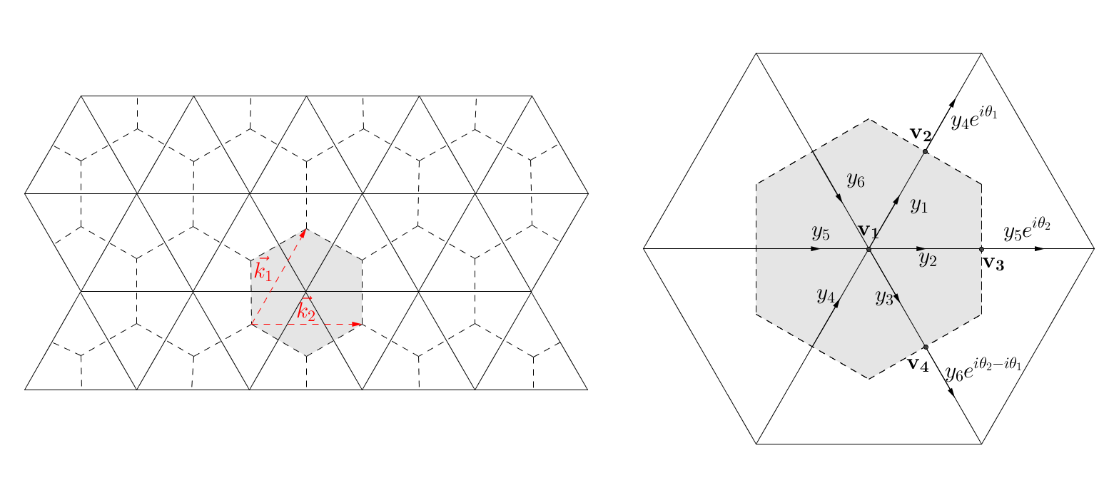
The fundamental domain for triangular tiling is quite different from that of hexagonal tiling. Its edges cut through the triangular edges. We let it be a regular hexagon that can be spread to the whole plane by two vectors k1→=(a2,32​a)\vec{k_{1}}=\left(\frac{a}{2},\frac{\sqrt{3}}{2}a\right) and k2→=(a,0)\vec{k_{2}}=(a,0) as shown in Figure 1.

Refer to caption
Figure 1: Fundamental domain for triangular tiling

Inside the domain, there are six functions (y1,⋯,y6y_{1},\cdots,y_{6}) to be determined. Assume that each equilateral triangle has edgelength aa. From Figure 1, we have first

−yi′′+qi​yi=λ​yi(i=1,…,6).-y_{i}^{\prime\prime}+q_{i}y_{i}=\lambda y_{i}\qquad(i=1,\ldots,6). (2.1)

With the Neumann vertex conditions, we find that at 𝐯1{\bf v}_{1},

{y1​(0)=y2​(0)=y3​(0)=y4​(a)=y5​(a)=y6​(a)y1′​(0)+y2′​(0)+y3′​(0)−y4′​(a)−y5′​(a)−y6′​(a)=0\left\{\begin{array}[]{l}y_{1}(0)=y_{2}(0)=y_{3}(0)=y_{4}(a)=y_{5}(a)=y_{6}(a)\\ y^{\prime}_{1}(0)+y^{\prime}_{2}(0)+y^{\prime}_{3}(0)-y^{\prime}_{4}(a)-y^{\prime}_{5}(a)-y^{\prime}_{6}(a)=0\end{array}\right. (2.2)

And at vertices 𝐯2{\bf v}_{2}, 𝐯3{\bf v}_{3}, and 𝐯5{\bf v}_{5}, by the Floquet-Bloch conditions,

{y1(a/2)=ei​θ1y4(a/2);y1′(a/2)+ei​θ1y4′(a/2)=0,y2(a/2)=ei​θ2y5(a/2);y2′(a/2)+ei​θ2y5′(a/2)=0,y3(a/2)=ei⁡(θ2−θ1)y6(a/2);y3′(a/2)+ei⁡(θ2−θ1)y6′(a/2)=0,\left\{\begin{array}[]{l}y_{1}(a/2)=e^{i\theta_{1}}y_{4}(a/2);\ y_{1}^{\prime}(a/2)+e^{i\theta_{1}}y_{4}^{\prime}(a/2)=0,\\ y_{2}(a/2)=e^{i\theta_{2}}y_{5}(a/2);\ y_{2}^{\prime}(a/2)+e^{i\theta_{2}}y_{5}^{\prime}(a/2)=0,\\ y_{3}(a/2)=e^{i(\theta_{2}-\theta_{1})}y_{6}(a/2);\ y_{3}^{\prime}(a/2)+e^{i(\theta_{2}-\theta_{1})}y_{6}^{\prime}(a/2)=0,\end{array}\right. (2.3)

This is because by periodicity, q1=q4q_{1}=q_{4}, q2=q5q_{2}=q_{5} and q3=q6q_{3}=q_{6}, and the edge e3e_{3} is just e6e_{6} translated by the vector k→3=k→2−k→1\vec{k}_{3}=\vec{k}_{2}-\vec{k}_{1}. Hence Hence, by the uniqueness of solutions, (2.3) implies that

y4​(x)=α​y1​(x);y5​(x)=β​y2​(x);y6​(x)=α​β−1​y3​(x).y_{4}(x)=\alpha y_{1}(x);\quad y_{5}(x)=\beta y_{2}(x);\quad y_{6}(x)=\alpha\beta^{-1}y_{3}(x).

where α=e−i​θ1\alpha=e^{-i\theta_{1}} and β=e−i​θ2\beta=e^{-i\theta_{2}}. Since yj=Aj​Cj+Bj​Sjy_{j}=A_{j}C_{j}+B_{j}S_{j}, the equations in (2.2) and (2.3) implies

{A1=A2=A3=α⁡(A1​C1+B1​S1)=β⁡(A2​C2+B2​S2)=α−1​β​(A3​C3+B3​S3),−B1−B2−B3+α⁡(A1​C1′+B1​S1′)+β⁡(A2​C2′+B2​S2′)+α−1​β​(A3​C3′+B3​S3′)=0.\left\{\begin{array}[]{l}A_{1}=A_{2}=A_{3}=\alpha(A_{1}C_{1}+B_{1}S_{1})=\beta(A_{2}C_{2}+B_{2}S_{2})=\alpha^{-1}\beta(A_{3}C_{3}+B_{3}S_{3}),\\ -B_{1}-B_{2}-B_{3}+\alpha(A_{1}C_{1}^{\prime}+B_{1}S_{1}^{\prime})+\beta(A_{2}C_{2}^{\prime}+B_{2}S_{2}^{\prime})+\alpha^{-1}\beta(A_{3}C_{3}^{\prime}+B_{3}S_{3}^{\prime})=0.\end{array}\right. (2.4)

This is a system of linear equations in (A1,A2,A3,B1,B2,B3)(A_{1},A_{2},A_{3},B_{1},B_{2},B_{3}). There is a solution if and only if the following determinant Φ⁡(ρ)\Phi(\rho) vanishes.

Φ⁡(ρ)=|−110000−101000−1+α​C100α​S100−1β​C200β​S20−10α−1​β​C300α−1​β​S3α​C1′β​C2′α−1​β​C3′−1+α​S1′−1+β​S2′−1+α−1​β​S3′|\Phi(\rho)=\begin{vmatrix}-1&1&0&0&0&0&\\ -1&0&1&0&0&0&\\ -1+\alpha C_{1}&0&0&\alpha S_{1}&0&0&\\ -1&\beta C_{2}&0&0&\beta S_{2}&0&\\ -1&0&\alpha^{-1}\beta C_{3}&0&0&\alpha^{-1}\beta S_{3}&\\ \alpha C_{1}^{\prime}&\beta C_{2}^{\prime}&\alpha^{-1}\beta C_{3}^{\prime}&-1+\alpha S_{1}^{\prime}&-1+\beta S_{2}^{\prime}&-1+\alpha^{-1}\beta S_{3}^{\prime}&\end{vmatrix}

We expand the above determinant with the help of the symbolic software Mathematica. Then we group the terms in order of αi​βj\alpha^{i}\beta^{j}, and invoke the Lagrange identity Cj​Sj′−Sj​Cj′=1C_{j}S_{j}^{\prime}-S_{j}C_{j}^{\prime}=1, to obtain

Φ⁡(ρ)\displaystyle\Phi(\rho) =\displaystyle= S1​S3​(β+β3)+S2​S3​(α−1​β2+α​β2)+S1​S2​(α​β+α−1​β3)−β2​(S1​S3​(C2+S2′)CLOSE\displaystyle S_{1}S_{3}(\beta+\beta^{3})+S_{2}S_{3}(\alpha^{-1}\beta^{2}+\alpha\beta^{2})+S_{1}S_{2}(\alpha\beta+\alpha^{-1}\beta^{3})-\beta^{2}(S_{1}S_{3}(C_{2}+S_{2}^{\prime})
+S2​S3​(C1+S1′)+S1​S2​(C3+S3′)\displaystyle+S_{2}S_{3}(C_{1}+S_{1}^{\prime})+S_{1}S_{2}(C_{3}+S_{3}^{\prime})
=\displaystyle= −e−2​i​θ2{(S1S2S3)′+(CSS)123−2S1S2cos(θ2−θ1)−2S2S3cosθ1\displaystyle-{\rm e}^{-2i\theta_{2}}\left\{(S_{1}S_{2}S_{3})^{\prime}+(CSS)_{123}-2S_{1}S_{2}\cos(\theta_{2}-\theta_{1})-2S_{2}S_{3}\cos\theta_{1}\right.
−2S1S3cosθ2}.\displaystyle\quad\left.-2S_{1}S_{3}\cos\theta_{2}\right\}.

In the above, we used some simple identities β2=e−2​i​θ2\beta^{2}={\rm e}^{-2i\theta_{2}}, and α+α−1=2cosθ1\alpha+\alpha^{-1}=2\cos\theta_{1}, while β+β−1=2cosθ2\beta+\beta^{-1}=2\cos\theta_{2}. The notation (C​S​S)123(CSS)_{123} was defined in (1.7).

Theorem 2.1.

For the periodic quantum graph associated with triangular tiling, the characteristic function is given by

Φ⁡(ρ)\displaystyle\Phi(\rho) =\displaystyle= −e−2​i​θ2{(S1S2S3)′+(CSS)123−2S1S2cos(θ2−θ1)−2S2S3cosθ1\displaystyle-{\rm e}^{-2i\theta_{2}}\left\{(S_{1}S_{2}S_{3})^{\prime}+(CSS)_{123}-2S_{1}S_{2}\cos(\theta_{2}-\theta_{1})-2S_{2}S_{3}\cos\theta_{1}\right.
−2S1S3cosθ2}.\displaystyle\quad\left.-2S_{1}S_{3}\cos\theta_{2}\right\}.

Assume that qq is even, then by Theorem 1.3(d), S′=CS^{\prime}=C. Therefore

Φ(ρ)=−2e−2​i​θ2((S1S2S3)′−S1S2cos(θ2−θ1)−S2S3cosθ1−S1S3cosθ2).\Phi(\rho)=-2{\rm e}^{-2i\theta_{2}}\left((S_{1}S_{2}S_{3})^{\prime}-S_{1}S_{2}\cos(\theta_{2}-\theta_{1})-S_{2}S_{3}\cos\theta_{1}-S_{1}S_{3}\cos\theta_{2}\right).

And if all the potentials are equal, we let Cj:=CC_{j}:=C and Sj:=SS_{j}:=S. Then the dispersion relation will be

S2​(3​S′−cos⁡(θ2−θ1)−cos⁡θ1−cos⁡θ2)=0.S^{2}\,\left(3S^{\prime}-\cos(\theta_{2}-\theta_{1})-\cos\theta_{1}-\cos\theta_{2}\right)=0.

Consequently by (1.6), the dispersion relation becomes

S2​(3​S′+1−4​cos⁡(θ12)​cos⁡(θ22)​cos⁡(θ2−θ12))=0.S^{2}\,\left(3S^{\prime}+1-4\cos(\frac{\theta_{1}}{2})\cos(\frac{\theta_{2}}{2})\cos(\frac{\theta_{2}-\theta_{1}}{2})\right)=0.

3 Elongated triangular tiling

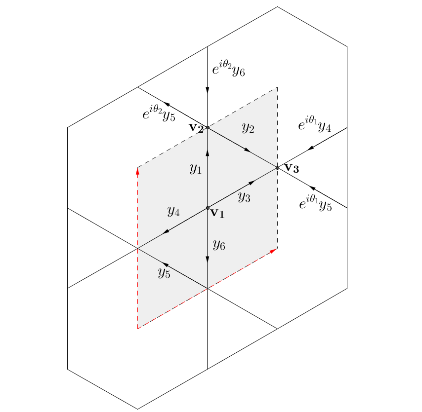
For this periodic graph associated with elongated triangular tiling with edgelength aa, we choose a fundamental domain as a hexagon as shown in Fig.2 that can be spread to the whole plane by two vectors k→1=(a,0)\vec{k}_{1}={(a,0)} and k→2=(a2,(1+32)​a)\vec{k}_{2}=\left(\frac{a}{2},(1+\frac{\sqrt{3}}{2})a\right). Thus k→3=k→1−k→2=(a2,−(1+32)​a)\displaystyle\vec{k}_{3}=\vec{k}_{1}-\vec{k}_{2}=(\frac{a}{2},-(1+\frac{\sqrt{3}}{2})a).

Refer to caption
Figure 2: Fundamental domain for elongated triangular tiling

Realizing the Neumann vertex condition at 𝐯1{\bf v}_{1},

{y1​(a)=y2​(a)=y2​(0)​ei​θ1=y3​(a)=y4​(a)y1′​(a)+y2′​(a)−y2′​(0)​ei​θ1+y3′​(a)+y4′​(a)=0.\begin{cases}&y_{1}(a)=y_{2}(a)=y_{2}(0)e^{i\theta_{1}}=y_{3}(a)=y_{4}(a)\\ &y^{\prime}_{1}(a)+y^{\prime}_{2}(a)-y^{\prime}_{2}(0)e^{i\theta_{1}}+y^{\prime}_{3}(a)+y^{\prime}_{4}(a)=0\end{cases}. (3.1)

Also, at the vertex 𝐯2{\bf v}_{2}, we have

{y4​(0)=y5​(a)=y3​(0)​ei​θ1=y5​(0)​ei​θ1=y1​(0)​ei​θ1−i​θ2y4′​(0)−y5′​(a)+y3′​(0)​ei​θ1+y5′​(0)​ei​θ1+y1′​(0)​ei​θ1−i​θ2=0.\begin{cases}&y_{4}(0)=y_{5}(a)=y_{3}(0)e^{i\theta_{1}}=y_{5}(0)e^{i\theta_{1}}=y_{1}(0)e^{i\theta_{1}-i\theta_{2}}\\ &y^{\prime}_{4}(0)-y^{\prime}_{5}(a)+y^{\prime}_{3}(0)e^{i\theta_{1}}+y^{\prime}_{5}(0)e^{i\theta_{1}}+y^{\prime}_{1}(0)e^{i\theta_{1}-i\theta_{2}}=0\end{cases}. (3.2)

Since yj=Aj​Cj+Bj​Sjy_{j}=A_{j}C_{j}+B_{j}S_{j}, we can rewrite (3.1)(\ref{1}) and (3.2)(\ref{2}) as a linear system of (A1,⋯,A5)(A_{1},\cdots,A_{5}) and (B1,⋯,B5)(B_{1},\cdots,B_{5}) with α~=ei​θ1\widetilde{\alpha}=e^{i\theta_{1}} and β=e−i​θ2\beta=e^{-i\theta_{2}}. Thus,

{A1​C1+B1​S1=A2​C2+B2​S2=A2​α~=A3​C3+B3​S3=A4​C4+B4​S4(A1​C1′+B1​S1′)+(A2​C2′+B2​S2′)−B2​α~+(A3​C3′+B3​S3′)+(A4​C4′+B4​S4′)=0A4=A5​C5+B5​S5=A3​α~=A5​α~=A1​α~​βB4−(A5​C5′+B5​S5′)+B3​α~+B5​α~+B1​α~​β=0.\begin{cases}&A_{1}C_{1}+B_{1}S_{1}=A_{2}C_{2}+B_{2}S_{2}=A_{2}\widetilde{\alpha}=A_{3}C_{3}+B_{3}S_{3}=A_{4}C_{4}+B_{4}S_{4}\\ &(A_{1}C^{\prime}_{1}+B_{1}S^{\prime}_{1})+(A_{2}C^{\prime}_{2}+B_{2}S^{\prime}_{2})-B_{2}\widetilde{\alpha}+(A_{3}C^{\prime}_{3}+B_{3}S^{\prime}_{3})+(A_{4}C^{\prime}_{4}+B_{4}S^{\prime}_{4})=0\\ &A_{4}=A_{5}C_{5}+B_{5}S_{5}=A_{3}\widetilde{\alpha}=A_{5}\widetilde{\alpha}=A_{1}\widetilde{\alpha}\beta\\ &B_{4}-(A_{5}C^{\prime}_{5}+B_{5}S^{\prime}_{5})+B_{3}\widetilde{\alpha}+B_{5}\widetilde{\alpha}+B_{1}\widetilde{\alpha}\beta=0\end{cases}.

So the characteristic equation Φ⁡(ρ)\Phi(\rho) is a determinant of 10×1010\times 10 matrix

Φ⁡(ρ)=|C1−α~000S100000C2−α~0000S20000−α~C30000S3000−α~0C40000S40C1′C2′C3′C4′0S1′S2′−α~S3′S4′0000−1C50000S500α~−1000000000−1α~00000α~​β00−10000000000−C5′α~​β0α~1α~−S5′|\Phi(\rho)=\begin{vmatrix}C_{1}&-\widetilde{\alpha}&0&0&0&S_{1}&0&0&0&0&\\ 0&C_{2}-\widetilde{\alpha}&0&0&0&0&S_{2}&0&0&0&\\ 0&-\widetilde{\alpha}&C_{3}&0&0&0&0&S_{3}&0&0&\\ 0&-\widetilde{\alpha}&0&C_{4}&0&0&0&0&S_{4}&0&\\ C^{\prime}_{1}&C^{\prime}_{2}&C^{\prime}_{3}&C^{\prime}_{4}&0&S^{\prime}_{1}&S^{\prime}_{2}-\widetilde{\alpha}&S^{\prime}_{3}&S^{\prime}_{4}&0&\\ 0&0&0&-1&C_{5}&0&0&0&0&S_{5}&\\ 0&0&\widetilde{\alpha}&-1&0&0&0&0&0&0&\\ 0&0&0&-1&\widetilde{\alpha}&0&0&0&0&0&\\ \widetilde{\alpha}\beta&0&0&-1&0&0&0&0&0&0&\\ 0&0&0&0&-C^{\prime}_{5}&\widetilde{\alpha}\beta&0&\widetilde{\alpha}&1&\widetilde{\alpha}-S^{\prime}_{5}\end{vmatrix}

The above matrix is complicated to handle by using manual computation. However, with the help of Mathematica, and the Lagrange identity, Cj​Sj′−Sj​Cj′=1C_{j}S_{j}^{\prime}-S_{j}C_{j}^{\prime}=1, it still comes up with a long expression. Grouping in terms of different powers of α~\widetilde{\alpha} and β~\widetilde{\beta}, we obtain

Φ⁡(ρ)=Ψ1+Ψ2+Ψ3+Ψ4,\Phi(\rho)=\Psi_{1}+\Psi_{2}+\Psi_{3}+\Psi_{4},

where, as α~2+1=2α~cosθ1\widetilde{\alpha}^{2}+1=2\widetilde{\alpha}\,\cos\theta_{1}, and 1+α~2​β2=2​α~​β​cos⁡(θ1−θ2)1+\widetilde{\alpha}^{2}\beta^{2}=2\widetilde{\alpha}\beta\,\cos(\theta_{1}-\theta_{2}),

Ψ1=−(α~6+α~2)​β​S1​S3​S4−2​α~4​β​S1​S3​S4=−4​α~4​β​cos2⁡θ1​S1​S3​S4,\Psi_{1}=-(\widetilde{\alpha}^{6}+\widetilde{\alpha}^{2})\beta S_{1}S_{3}S_{4}-2\widetilde{\alpha}^{4}\beta S_{1}S_{3}S_{4}=-4\widetilde{\alpha}^{4}\beta\cos^{2}\theta_{1}\,S_{1}S_{3}S_{4},

while

Ψ2\displaystyle\Psi_{2} =\displaystyle= (α~5+α~3)​β​(S1′​S2​S3​S4+S2′​S1​S3​S4+S3′​S1​S2​S4+S4′​S1​S2​S3+S5′​S1​S3​S4CLOSE\displaystyle(\widetilde{\alpha}^{5}+\widetilde{\alpha}^{3})\beta\left(S_{1}^{\prime}S_{2}S_{3}S_{4}+S_{2}^{\prime}S_{1}S_{3}S_{4}+S_{3}^{\prime}S_{1}S_{2}S_{4}+S_{4}^{\prime}S_{1}S_{2}S_{3}+S_{5}^{\prime}S_{1}S_{3}S_{4}\right.
OPEN+C1​S3​S4​S5+C2​S1​S3​S4+C3​S1​S4​S5+C4​S1​S3​S5+C5​S1​S3​S4)\displaystyle\left.+C_{1}S_{3}S_{4}S_{5}+C_{2}S_{1}S_{3}S_{4}+C_{3}S_{1}S_{4}S_{5}+C_{4}S_{1}S_{3}S_{5}+C_{5}S_{1}S_{3}S_{4}\right)
=\displaystyle= 2α4βcosθ1((S1S2S3S4)′+(CSSS)1345+S1S3S4(C2+S5′));\displaystyle 2\alpha^{4}\beta\cos\theta_{1}\,\left((S_{1}S_{2}S_{3}S_{4})^{\prime}+(CSSS)_{1345}+S_{1}S_{3}S_{4}(C_{2}+S_{5}^{\prime})\right)\ ;
Ψ3\displaystyle\Psi_{3} =\displaystyle= (α~5+α~3)​β​S1​S2​S5+(α~3+α~5​β2)​S2​S3​S5+α~4​(1+β2)​S2​S4​S5\displaystyle(\widetilde{\alpha}^{5}+\widetilde{\alpha}^{3})\beta S_{1}S_{2}S_{5}+(\widetilde{\alpha}^{3}+\widetilde{\alpha}^{5}\beta^{2})S_{2}S_{3}S_{5}+\widetilde{\alpha}^{4}(1+\beta^{2})S_{2}S_{4}S_{5}
=\displaystyle= 2α~4β(S1S2S5cosθ1+S2S3S5cos(θ1−θ2)+S2S4S5cosθ2).\displaystyle 2\widetilde{\alpha}^{4}\beta\,\left(S_{1}S_{2}S_{5}\cos\theta_{1}+S_{2}S_{3}S_{5}\cos(\theta_{1}-\theta_{2})+S_{2}S_{4}S_{5}\cos\theta_{2}\right).

The last part is most tedious. But we follow the pattern of the above main terms and succeed in grouping them as follows:

Ψ4\displaystyle\Psi_{4} =\displaystyle= −α~4β[S1′S5′S2S3S4+S2′S5′S1S3S4+S3′S5′S1S2S4\displaystyle-\widetilde{\alpha}^{4}\beta\left[S_{1}^{\prime}S_{5}^{\prime}S_{2}S_{3}S_{4}+S_{2}^{\prime}S_{5}^{\prime}S_{1}S_{3}S_{4}+S_{3}^{\prime}S_{5}^{\prime}S_{1}S_{2}S_{4}\right.
+S4′​S5′​S1​S2​S3+C1′​S2​S3​S4​S5+C3′​S1​S2​S4​S5+C4′​S1​S2​S3​S5+S1′​C3​S2​S4​S5+S1′​C4​S2​S3​S5\displaystyle\left.+S_{4}^{\prime}S_{5}^{\prime}S_{1}S_{2}S_{3}+C_{1}^{\prime}S_{2}S_{3}S_{4}S_{5}+C_{3}^{\prime}S_{1}S_{2}S_{4}S_{5}+C_{4}^{\prime}S_{1}S_{2}S_{3}S_{5}+S_{1}^{\prime}C_{3}S_{2}S_{4}S_{5}+S_{1}^{\prime}C_{4}S_{2}S_{3}S_{5}\right.
+S1′​C5​S2​S3​S4+S2′​C1​S3​S4​S5+S2′​C3​S1​S4​S5+S2′​C4​S1​S3​S5+S2′​C5​S1​S3​S4+S3′​C1​S2​S4​S5\displaystyle\left.+S_{1}^{\prime}C_{5}S_{2}S_{3}S_{4}+S_{2}^{\prime}C_{1}S_{3}S_{4}S_{5}+S_{2}^{\prime}C_{3}S_{1}S_{4}S_{5}+S_{2}^{\prime}C_{4}S_{1}S_{3}S_{5}+S_{2}^{\prime}C_{5}S_{1}S_{3}S_{4}+S_{3}^{\prime}C_{1}S_{2}S_{4}S_{5}\right.
+S3′​C4​S1​S2​S5+S3′​C5​S1​S2​S4+S4′​C1​S2​S3​S5+S4′​C3​S1​S2​S5+S4′​C5​S1​S2​S3+S5′​C2​S1​S3​S4\displaystyle\left.+S_{3}^{\prime}C_{4}S_{1}S_{2}S_{5}+S_{3}^{\prime}C_{5}S_{1}S_{2}S_{4}+S_{4}^{\prime}C_{1}S_{2}S_{3}S_{5}+S_{4}^{\prime}C_{3}S_{1}S_{2}S_{5}+S_{4}^{\prime}C_{5}S_{1}S_{2}S_{3}+S_{5}^{\prime}C_{2}S_{1}S_{3}S_{4}\right.
+C1C2S3S4S5+C2C3S1S4S5+C2C4S1S3S5+C2C5S1S3S4]\displaystyle\left.+C_{1}C_{2}S_{3}S_{4}S_{5}+C_{2}C_{3}S_{1}S_{4}S_{5}+C_{2}C_{4}S_{1}S_{3}S_{5}+C_{2}C_{5}S_{1}S_{3}S_{4}\right]
=\displaystyle= −α~4β[(S1S2S3S4)′(C5+S5′)+(CSSS)1345(S2′+C2)+S1S2S5((C4S3)′+(C3S4)′)\displaystyle{-\widetilde{\alpha}^{4}\beta}\left[(S_{1}S_{2}S_{3}S_{4})^{\prime}(C_{5}+S_{5}^{\prime})+(CSSS)_{1345}(S_{2}^{\prime}+C_{2})+S_{1}S_{2}S_{5}((C_{4}S_{3})^{\prime}+(C_{3}S_{4})^{\prime})\right.
+S2S3S5(C4S1′+(C1S4)′)+S2S4S5(S1′C3+C1S3′)+S1S3S4(C2S5′−S2′C5)]\displaystyle\left.+S_{2}S_{3}S_{5}(C_{4}S_{1}^{\prime}+(C_{1}S_{4})^{\prime})+S_{2}S_{4}S_{5}({S^{\prime}_{1}C_{3}}+C_{1}S_{3}^{\prime})+S_{1}S_{3}S_{4}(C_{2}S_{5}^{\prime}-S_{2}^{\prime}C_{5})\right]

Therefore, we have the following formula for the characteristic function:

Theorem 3.1.

For the periodic quantum graph of elongated triangular tiling with length aa, we have

Φ⁡(ρ)\displaystyle\Phi(\rho) =\displaystyle= −α~4β{(S1S2S3S4)′(C5+S5′−2cosθ1)+(CSSS)1345(S2′+C2−2cosθ1)\displaystyle-\widetilde{\alpha}^{4}\beta\{(S_{1}S_{2}S_{3}S_{4})^{\prime}(C_{5}+S_{5}^{\prime}-2\cos\theta_{1})+(CSSS)_{1345}(S_{2}^{\prime}+C_{2}-2\cos\theta_{1})
+S1S2S5((C4S3)′+(C3S4)′−2cosθ1)+S2S3S5((C1S4)′+S1′C4−2cos(θ1−θ2))\displaystyle+S_{1}S_{2}S_{5}((C_{4}S_{3})^{\prime}+(C_{3}S_{4})^{\prime}-2\cos\theta_{1})+S_{2}S_{3}S_{5}((C_{1}S_{4})^{\prime}+S_{1}^{\prime}C_{4}-2\cos(\theta_{1}-\theta_{2}))
+S2S4S5(S1′C3+C1S3′−2cosθ2)+S1S3S4(C2S5′−S2′C5−2(C2+S5′)cosθ1+4cos2θ1)}\displaystyle+S_{2}S_{4}S_{5}({S^{\prime}_{1}C_{3}}+C_{1}S_{3}^{\prime}-2\cos\theta_{2})+S_{1}S_{3}S_{4}(C_{2}S_{5}^{\prime}-S_{2}^{\prime}C_{5}-2(C_{2}+S_{5}^{\prime})\cos\theta_{1}{+}4\cos^{2}\theta_{1})\}

Note that in Theorem 3.1, the involved quantum graph has different potential functions on distinct edges. If all the potentials are equal, then we let Cj:=CC_{j}:=C and Sj:=SS_{j}:=S. The dispersion relation is given by

0\displaystyle 0 =\displaystyle= S3{2cosθ1+2cosθ2+2cos(θ1−θ2)+3+10S′cosθ1+10Ccosθ1−4cos2θ1\displaystyle S^{3}\{2\cos\theta_{1}+2\cos\theta_{2}+2\cos(\theta_{1}-\theta_{2})+3+10S^{\prime}\cos\theta_{1}+10C\cos\theta_{1}-4\cos^{2}\theta_{1}
−17S′C−4(S′)2−4C2}\displaystyle-17S^{\prime}C-4(S^{\prime})^{2}-4C^{2}\}

If we further assume that the potentials are even, then by Theorem 1.3(d), the dispersion relation becomes

0\displaystyle 0 =\displaystyle= S3{25(S′)2−20cosθ1S′−2cosθ1−2cosθ2−2cos(θ1−θ2)+4cos2θ1−3}\displaystyle S^{3}\{25(S^{\prime})^{2}-20\cos\theta_{1}S^{\prime}-2\cos\theta_{1}-2\cos\theta_{2}-2\cos(\theta_{1}-\theta_{2})+4\cos^{2}\theta_{1}-3\}
=\displaystyle= S3{25(S′)2−20cosθ1S′−8cos(θ12)cos(θ22)cos(θ1−θ22)+4cos2θ1−1},\displaystyle S^{3}\{25(S^{\prime})^{2}-20\cos\theta_{1}S^{\prime}-8\cos(\frac{\theta_{1}}{2})\cos(\frac{\theta_{2}}{2})\cos(\frac{\theta_{1}-\theta_{2}}{2})+4\cos^{2}\theta_{1}-1\},

by (1.6). This proves Theorem 1.1(b).

4 Truncated square tiling

For this periodic quantum graph associated with truncated square tiling with edgelength aa, we choose a fundamental domain as a square spanned by two vectors k→1=(0,(1+2)​a)\vec{k}_{1}=\left(0,(1+\sqrt{2})a\right) and k→2=((1+2)​a,0)\vec{k}_{2}=\left((1+\sqrt{2})a,0\right) as shown in the figure below.

Refer to caption
Figure 3: Fundamental domain for truncated square tiling

We first note that by the Floquet-Bloch conditions, y7​(x)=ei​θ1​y5​(x)y_{7}(x)={\rm e}^{i\theta_{1}}y_{5}(x), and y8​(x)=ei​θ2​y6​(x)y_{8}(x)={\rm e}^{i\theta_{2}}y_{6}(x). Next the Neumann vertex conditions at vertex 𝐯1{\bf v}_{1} imply

{y1​(0)=y4​(0)=y5​(0)y1′​(0)+y4′​(0)+y5′​(0)=0.\begin{cases}&y_{1}(0)=y_{4}(0)=y_{5}(0)\\ &y^{\prime}_{1}(0)+y^{\prime}_{4}(0)+y^{\prime}_{5}(0)=0\end{cases}.

At the vertex v2,

{y1​(a)=y2​(a)=y6​(0)y1′​(a)+y2′​(a)−y6′​(0)=0.\begin{cases}&y_{1}(a)=y_{2}(a)=y_{6}(0)\\ &y^{\prime}_{1}(a)+y^{\prime}_{2}(a)-y^{\prime}_{6}(0)=0\end{cases}.

At vertex v3, they become

{y2​(0)=y3​(0)=ei​θ1​y5​(a)y2′​(0)+y3′​(0)−ei​θ1​y5​(a)=0;\begin{cases}&y_{2}(0)=y_{3}(0)={\rm e}^{i\theta_{1}}y_{5}(a)\\ &y^{\prime}_{2}(0)+y^{\prime}_{3}(0)-{\rm e}^{i\theta_{1}}y_{5}(a)=0\end{cases};

and

{y3​(a)=y4​(a)=ei​θ2​y6​(a)y3′​(a)+y4′​(a)+ei​θ2​y6′​(a)=0.\begin{cases}&y_{3}(a)=y_{4}(a)={\rm e}^{i\theta_{2}}y_{6}(a)\\ &y^{\prime}_{3}(a)+y^{\prime}_{4}(a)+{\rm e}^{i\theta_{2}}y^{\prime}_{6}(a)=0\end{cases}.

Since yj=Aj​Cj+Bj​Sjy_{j}=A_{j}C_{j}+B_{j}S_{j}, we can rewrite the above equations as a linear system of (A1,⋯,A6)(A_{1},\cdots,A_{6}) and (B1,⋯,B6)(B_{1},\cdots,B_{6}) with α~=ei​θ1\widetilde{\alpha}=e^{i\theta_{1}} and β~=ei​θ2\widetilde{\beta}=e^{i\theta_{2}}. Thus,

{A1=A4=A5B1+B4+B5=0A6=A1​C1+B1​S1=A2​C2+B2​S2B6−A1​C1′−B1​S1′−A2​C2′−B2​S2=0A2=A3=ei​θ1​(A5​C5+B5​C5)B2+B3−ei​θ1​(A5​C5′+B5​S5′)=0ei​θ2​(A6​C6+B6​S6)=A3​C3+B3​S3=A4​C4+B4​S4ei​θ2​(A6​C6′+B6​S6′)+A3​C3′+B3​S3′+A4​C4′+B4​S4′=0.\begin{cases}&A_{1}=A_{4}=A_{5}\\ &B_{1}+B_{4}+B_{5}=0\\ &A_{6}=A_{1}C_{1}+B_{1}S_{1}=A_{2}C_{2}+B_{2}S_{2}\\ &B_{6}-A_{1}C_{1}^{\prime}-B_{1}S_{1}^{\prime}-A_{2}C_{2}^{\prime}-B_{2}S_{2}=0\\ &A_{2}=A_{3}={\rm e}^{i\theta_{1}}(A_{5}C_{5}+B_{5}C_{5})\\ &B_{2}+B_{3}-{\rm e}^{i\theta_{1}}(A_{5}C_{5}^{\prime}+B_{5}S_{5}^{\prime})=0\\ &{\rm e}^{i\theta_{2}}(A_{6}C_{6}+B_{6}S_{6})=A_{3}C_{3}+B_{3}S_{3}=A_{4}C_{4}+B_{4}S_{4}\\ &{\rm e}^{i\theta_{2}}(A_{6}C_{6}^{\prime}+B_{6}S_{6}^{\prime})+A_{3}C_{3}^{\prime}+B_{3}S_{3}^{\prime}+A_{4}C_{4}^{\prime}+B_{4}S_{4}^{\prime}=0\end{cases}.

So the characteristic equation Φ⁡(ρ)\Phi(\rho) is a determinant of 12×1212\times 12 matrix

Φ⁡(ρ)=|100−1000S100001000−10000000000000100110C10000−1S1000000C2000−10S20000C1′C2′0000S1′S2′000−101−10000000000−100α​C500000α​S500000α​C5′0−1−100α​S5′000−C3C40000−S3S40000−C300β​C600−S300β​S600C3′C4′0β​C6′00S3′S4′0β​S6′|\Phi(\rho)=\scriptsize{\begin{vmatrix}1&0&0&-1&0&0&0&S_{1}&0&0&0&0&\\ 1&0&0&0&-1&0&0&0&0&0&0&0&\\ 0&0&0&0&0&0&1&0&0&1&1&0&\\ C_{1}&0&0&0&0&-1&S_{1}&0&0&0&0&0&\\ 0&C_{2}&0&0&0&-1&0&S_{2}&0&0&0&0\\ C^{\prime}_{1}&C^{\prime}_{2}&0&0&0&0&S^{\prime}_{1}&S^{\prime}_{2}&0&0&0&-1&\\ 0&1&-1&0&0&0&0&0&0&0&0&0&\\ 0&-1&0&0&\alpha C_{5}&0&0&0&0&0&\alpha S_{5}&0&\\ 0&0&0&0&\alpha C_{5}^{\prime}&0&-1&-1&0&0&\alpha S_{5}^{\prime}&0&\\ 0&0&-C_{3}&C_{4}&0&0&0&0&-S_{3}&S_{4}&0&0&\\ 0&0&-C_{3}&0&0&\beta C_{6}&0&0&-S_{3}&0&0&\beta S_{6}&\\ 0&0&C_{3}^{\prime}&C_{4}^{\prime}&0&\beta C_{6}^{\prime}&0&0&S_{3}^{\prime}&S_{4}^{\prime}&0&\beta S_{6}^{\prime}&\end{vmatrix}}

The above matrix is complicated to handle by using manual computation. However, with the help of Mathematica, we manage to simplify the expression using the Lagrange identity, CjSj′−SjCj′=1,∀j=1,⋯,5C_{j}S_{j}^{\prime}-S_{j}C_{j}^{\prime}=1,\forall j=1,\cdots,5. It still comes up with a long expression. Grouping in terms of different powers of α~\widetilde{\alpha} and β~\widetilde{\beta}, we obtain

−Φ⁡(ρ)=Ψ1+Ψ2+Ψ3+Ψ4,-\Phi(\rho)=\Psi_{1}+\Psi_{2}+\Psi_{3}+\Psi_{4},

where

Ψ1=(1+α~2​β~2)​S1​S3+(α~2+β~2)​S2​S4​2​S2​S4​cos⁡(θ1−θ2)+2​S1​S3​cos⁡(θ1+θ2),\Psi_{1}=(1+\widetilde{\alpha}^{2}\widetilde{\beta}^{2})S_{1}S_{3}+(\widetilde{\alpha}^{2}+\widetilde{\beta}^{2})S_{2}S_{4}2S_{2}S_{4}\cos(\theta_{1}-\theta_{2})+2S_{1}S_{3}\cos(\theta_{1}+\theta_{2}),

while

Ψ2\displaystyle\Psi_{2} =\displaystyle= (1+α~2)​β~​(C6​S1​S2+S1​S6​S2′+S2​S6​S1′+S4​S6​S3′+S3​S6​S4′+S3​S4​S6′)\displaystyle(1+\widetilde{\alpha}^{2})\widetilde{\beta}(C_{6}S_{1}S_{2}+S_{1}S_{6}S_{2}^{\prime}+S_{2}S_{6}S_{1}^{\prime}+S_{4}S_{6}S_{3}^{\prime}+S_{3}S_{6}S_{4}^{\prime}+S_{3}S_{4}S_{6}^{\prime})
=\displaystyle= 2α~β~cosθ1((S3S4S6)′+S6(S1S2)′+C6S1S2)\displaystyle 2\widetilde{\alpha}\widetilde{\beta}\cos\theta_{1}\,\left((S_{3}S_{4}S_{6})^{\prime}+S_{6}(S_{1}S_{2})^{\prime}+C_{6}S_{1}S_{2}\right)\,
Ψ3\displaystyle\Psi_{3} =\displaystyle= α~​(1+β~2)​(C5​S1​S4+C4​S1​S5+C3​S2​S5+C2​S3​S5+C1​S4​S5+S2​S3​S5′)\displaystyle\widetilde{\alpha}(1+\widetilde{\beta}^{2})(C_{5}S_{1}S_{4}+C_{4}S_{1}S_{5}+C_{3}S_{2}S_{5}+C_{2}S_{3}S_{5}+C_{1}S_{4}S_{5}+S_{2}S_{3}S_{5}^{\prime})
=\displaystyle= 2α~β~cosθ2((CSS)145−S5(CS)23−S2S3S5′).\displaystyle 2\widetilde{\alpha}\widetilde{\beta}\cos\theta_{2}\,\left((CSS)_{145}-S_{5}(CS)_{23}-S_{2}S_{3}S_{5}^{\prime}\right).

Finally, Ψ4\Psi_{4} is the most tedious part.

Ψ4\displaystyle\Psi_{4} =\displaystyle= α~​β~​(−2​S5​S6+C1​C6​S2​S4​S5​C3′+S2​S4​S5​S6​C1′​C3′+C3​C6​S1​S2​S5​C4′+C2​C6​S1​S3​S5​C4′+S1​S3​S5​S6​C2′​C4′CLOSE\displaystyle\widetilde{\alpha}\widetilde{\beta}(-2S_{5}S_{6}+C_{1}C_{6}S_{2}S_{4}S_{5}C_{3}^{\prime}+S_{2}S_{4}S_{5}S_{6}C_{1}^{\prime}C_{3}^{\prime}+C_{3}C_{6}S_{1}S_{2}S_{5}C_{4}^{\prime}+C_{2}C_{6}S_{1}S_{3}S_{5}C_{4}^{\prime}+S_{1}S_{3}S_{5}S_{6}C_{2}^{\prime}C_{4}^{\prime}
+C1​C3​S2​S4​S5​C6′​C3​S2​S5​S6​C4′​S1′+C2​S3​S5​S6​C4′​S1′+C1​S4​S5​S6​C3′​S2′+C3​S1​S5​S6​C4′​S2′+C1​C2​C6​S4​S5​S3′\displaystyle+C_{1}C_{3}S_{2}S_{4}S_{5}C_{6}^{\prime}C_{3}S_{2}S_{5}S_{6}C_{4}^{\prime}S_{1}^{\prime}+C_{2}S_{3}S_{5}S_{6}C_{4}^{\prime}S_{1}^{\prime}+C_{1}S_{4}S_{5}S_{6}C_{3}^{\prime}S_{2}^{\prime}+C_{3}S_{1}S_{5}S_{6}C_{4}^{\prime}S_{2}^{\prime}+C_{1}C_{2}C_{6}S_{4}S_{5}S_{3}^{\prime}
+C2​S4​S5​S6​C1′​S3′+C1​S4​S5​S6​C2′​S3′+C6​S1​S2​S4​C5′​S3′+S2​S4​S6​C5′​S1′​S3′+S1​S4​S6​C5′​S2′​S3′+C1​C3​C6​S2​S5​S4′\displaystyle+C_{2}S_{4}S_{5}S_{6}C_{1}^{\prime}S_{3}^{\prime}+C_{1}S_{4}S_{5}S_{6}C_{2}^{\prime}S_{3}^{\prime}+C_{6}S_{1}S_{2}S_{4}C_{5}^{\prime}S_{3}^{\prime}+S_{2}S_{4}S_{6}C_{5}^{\prime}S_{1}^{\prime}S_{3}^{\prime}+S_{1}S_{4}S_{6}C_{5}^{\prime}S_{2}^{\prime}S_{3}^{\prime}+C_{1}C_{3}C_{6}S_{2}S_{5}S_{4}^{\prime}
+C1​C2​C​C6​S3​S5​S4′+C3​S2​S5​S6​C1′​S4′+C2​S3​S5​S6​C1′​S4′+C1​S3​S5​S6​C2′​S4′+C6​S1​S2​S3​C5′​S4′+S2​S3​S6​C5′​S1′​S4′\displaystyle+C_{1}C_{2}CC_{6}S_{3}S_{5}S_{4}^{\prime}+C_{3}S_{2}S_{5}S_{6}C_{1}^{\prime}S_{4}^{\prime}+C_{2}S_{3}S_{5}S_{6}C_{1}^{\prime}S_{4}^{\prime}+C_{1}S_{3}S_{5}S_{6}C_{2}^{\prime}S_{4}^{\prime}+C_{6}S_{1}S_{2}S_{3}C_{5}^{\prime}S_{4}^{\prime}+S_{2}S_{3}S_{6}C_{5}^{\prime}S_{1}^{\prime}S_{4}^{\prime}
+C1​C3​S5​S6​S2′​S4′+S1​S3​C6​C5′​S2′​S4′+C6​S1​S2​S3​C4′​S5′+C1​S2​S3​S4​C6′​S5′+S2​S3​S6​C4′​S1′​S4′+S1​S3​S6​C4′​S2′​S5′\displaystyle+C_{1}C_{3}S_{5}S_{6}S_{2}^{\prime}S_{4}^{\prime}+S_{1}S_{3}C_{6}C_{5}^{\prime}S_{2}^{\prime}S_{4}^{\prime}+C_{6}S_{1}S_{2}S_{3}C_{4}^{\prime}S_{5}^{\prime}+C_{1}S_{2}S_{3}S_{4}C_{6}^{\prime}S_{5}^{\prime}+S_{2}S_{3}S_{6}C_{4}^{\prime}S_{1}^{\prime}S_{4}^{\prime}+S_{1}S_{3}S_{6}C_{4}^{\prime}S_{2}^{\prime}S_{5}^{\prime}
+C1​C6​S2​S4​S3′​S5′+S2​S4​S6​C1′​S3′​S5′+C1​S4​S6​S2′​S3′​S5′​C1​C6​S2​S3​S4′​S5′+S2​S3​S6​C1′​S4′​S5′+C1​S3​S6​S2′​S4′​S5′\displaystyle+C_{1}C_{6}S_{2}S_{4}S_{3}^{\prime}S_{5}^{\prime}+S_{2}S_{4}S_{6}C_{1}^{\prime}S_{3}^{\prime}S_{5}^{\prime}+C_{1}S_{4}S_{6}S_{2}^{\prime}S_{3}^{\prime}S_{5}^{\prime}C_{1}C_{6}S_{2}S_{3}S_{4}^{\prime}S_{5}^{\prime}+S_{2}S_{3}S_{6}C_{1}^{\prime}S_{4}^{\prime}S_{5}^{\prime}+C_{1}S_{3}S_{6}S_{2}^{\prime}S_{4}^{\prime}S_{5}^{\prime}
+C3​S2​S4​S5​C1′​S6′+C2​S3​S4​S5​C1′​S6′+C1​S3​S4​S5​C2′​S6′+S2​S3​S4​C5′​S1′​S6′+C1​C3​S4​S5​S2′​S6′+S1​S3​S4​C5′​S2′​S6′\displaystyle+C_{3}S_{2}S_{4}S_{5}C_{1}^{\prime}S_{6}^{\prime}+C_{2}S_{3}S_{4}S_{5}C_{1}^{\prime}S_{6}^{\prime}+C_{1}S_{3}S_{4}S_{5}C_{2}^{\prime}S_{6}^{\prime}+S_{2}S_{3}S_{4}C_{5}^{\prime}S_{1}^{\prime}S_{6}^{\prime}+C_{1}C_{3}S_{4}S_{5}S_{2}^{\prime}S_{6}^{\prime}+S_{1}S_{3}S_{4}C_{5}^{\prime}S_{2}^{\prime}S_{6}^{\prime}
+S2​S3​S4​C1′​S5′​S6′+C1​S3​S4​S2′​S5′​S6′+C4​(C2​S1​S3​S5​C6′+S2​S5​S6​C3′​S1′+S1​S5​S6​C3′​S2′+S1​S5​S6​C2′​S3′CLOSE\displaystyle+S_{2}S_{3}S_{4}C_{1}^{\prime}S_{5}^{\prime}S_{6}^{\prime}+C_{1}S_{3}S_{4}S_{2}^{\prime}S_{5}^{\prime}S_{6}^{\prime}+C_{4}\,(C_{2}S_{1}S_{3}S_{5}C_{6}^{\prime}+S_{2}S_{5}S_{6}C_{3}^{\prime}S_{1}^{\prime}+S_{1}S_{5}S_{6}C_{3}^{\prime}S_{2}^{\prime}+S_{1}S_{5}S_{6}C_{2}^{\prime}S_{3}^{\prime}
+C2​S5​S6​S1′​S3′+S1​S2​S3​C6′​S5′+S2​S6​S1′​S3′​S5′+S1​S6​S2′​S3′​S5′+C6​S1​(C2​S5​S3′+S2​(S5​C3′+S3′​S5′))\displaystyle+C_{2}S_{5}S_{6}S_{1}^{\prime}S_{3}^{\prime}+S_{1}S_{2}S_{3}C_{6}^{\prime}S_{5}^{\prime}+S_{2}S_{6}S_{1}^{\prime}S_{3}^{\prime}S_{5}^{\prime}+S_{1}S_{6}S_{2}^{\prime}S_{3}^{\prime}S_{5}^{\prime}+C_{6}S_{1}(C_{2}S_{5}S_{3}^{\prime}+S_{2}(S_{5}C_{3}^{\prime}+S_{3}^{\prime}S_{5}^{\prime}))
OPEN+S1​S3​S5​C2′​S6′+C2​S3​S5​S1′​S6′+S2​S3​S1′​S5′​S6′+S1​S3​S2′​S5′​S6′+C3​S5​(S2​S1′​S6′+S1​(S2​C6′+S2′​S6′)))\displaystyle+S_{1}S_{3}S_{5}C_{2}^{\prime}S_{6}^{\prime}+C_{2}S_{3}S_{5}S_{1}^{\prime}S_{6}^{\prime}+S_{2}S_{3}S_{1}^{\prime}S_{5}^{\prime}S_{6}^{\prime}+S_{1}S_{3}S_{2}^{\prime}S_{5}^{\prime}S_{6}^{\prime}+C_{3}S_{5}(S_{2}S_{1}^{\prime}S_{6}^{\prime}+S_{1}(S_{2}C_{6}^{\prime}+S_{2}^{\prime}S_{6}^{\prime})))
+C5​(C2​S1​S3​S4​C6′+S2​S4​S6​C3′​S1′+S1​S4​S6​C3′​S2′+S1​S4​S6​C2′​S3′+C2​S4​S6​S1′​S3′+S1​S3​S6​C2′​S4′CLOSE\displaystyle+C_{5}\,(C_{2}S_{1}S_{3}S_{4}C_{6}^{\prime}+S_{2}S_{4}S_{6}C_{3}^{\prime}S_{1}^{\prime}+S_{1}S_{4}S_{6}C_{3}^{\prime}S_{2}^{\prime}+S_{1}S_{4}S_{6}C_{2}^{\prime}S_{3}^{\prime}+C_{2}S_{4}S_{6}S_{1}^{\prime}S_{3}^{\prime}+S_{1}S_{3}S_{6}C_{2}^{\prime}S_{4}^{\prime}
+C2​S3​S6​S1′​S4′+C6​S1​(S2​(S4​C3′+C3​S4′)+C2​(S4​S3′+S3​S4′))+S1​S3​S4​C2′​S6′+C2​S3​S4​S1′​S6′\displaystyle+C_{2}S_{3}S_{6}S_{1}^{\prime}S_{4}^{\prime}+C_{6}S_{1}(S_{2}(S_{4}C_{3}^{\prime}+C_{3}S_{4}^{\prime})+C_{2}(S_{4}S_{3}^{\prime}+S_{3}S_{4}^{\prime}))+S_{1}S_{3}S_{4}C_{2}^{\prime}S_{6}^{\prime}+C_{2}S_{3}S_{4}S_{1}^{\prime}S_{6}^{\prime}
OPENOPEN+C3​(S2​S1′​(S6​S4′+S4​S6′)+S1​(S2​S4​C6′+S2′​(S6​S4′+S4​S6′)))))\displaystyle+C_{3}(S_{2}S_{1}^{\prime}(S_{6}S_{4}^{\prime}+S_{4}S_{6}^{\prime})+S_{1}(S_{2}S_{4}C_{6}^{\prime}+S_{2}^{\prime}(S_{6}S_{4}^{\prime}+S_{4}S_{6}^{\prime})))))

We follow the pattern of the above main terms and succeed in grouping them, as follows:

Ψ4\displaystyle\Psi_{4} =\displaystyle= (S5​S2​S3+S5​(C​S)23)​(C1′​(S4​S6)′+S1′​(C4​S6)′+S1​(C4​C6)′+C1​(S4​C6)′)+(C​S​S)145​(S2′​(C3​S6)′+C2′​(S3​S6)′CLOSE\displaystyle(S_{5}S_{2}S_{3}+S_{5}(CS)_{23})\,(C_{1}^{\prime}(S_{4}S_{6})^{\prime}+S_{1}^{\prime}(C_{4}S_{6})^{\prime}+S_{1}(C_{4}C_{6})^{\prime}+C_{1}(S_{4}C_{6})^{\prime})+(CSS)_{145}\,(S_{2}^{\prime}(C_{3}S_{6})^{\prime}+C_{2}^{\prime}(S_{3}S_{6})^{\prime}
OPEN+C6​(C​S)23′)+(C6​S1​S2+S6​(S1​S2)′)​(C5′​(S3​S4)′+C3​S4′​C5+S3′​C4​S5′)+(S3​S4​S6)′​(C1​S2′​S5′+S1′​C2​C5)\displaystyle+C_{6}(CS)_{23^{\prime}})+(C_{6}S_{1}S_{2}+S_{6}(S_{1}S_{2})^{\prime})\,(C_{5}^{\prime}(S_{3}S_{4})^{\prime}+C_{3}S_{4}^{\prime}C_{5}+S_{3}^{\prime}C_{4}S_{5}^{\prime})+(S_{3}S_{4}S_{6})^{\prime}\,(C_{1}S_{2}^{\prime}S_{5}^{\prime}+S_{1}^{\prime}C_{2}C_{5})
+S5​S6​((S​C)14′​(S​C)32′+(S​C)41′​(S​C)23′)+S2​S4​((S1′​S6′+S1​C6′)​(C3​C5+S3​C5′)CLOSE\displaystyle+S_{5}S_{6}\,((SC)_{14^{\prime}}(SC)_{32^{\prime}}+(SC)_{41^{\prime}}(SC)_{23^{\prime}})+S_{2}S_{4}\,((S_{1}^{\prime}S_{6}^{\prime}+S_{1}C_{6}^{\prime})(C_{3}C_{5}+S_{3}C_{5}^{\prime})
OPEN+S6​(C1′​S3′​S5′+S1′​C3′​C5)+C1​C6​S3′​S5′)+S1​S3​(S2′​S6′​(C​S)45′+C2​C5​(S4​S6)′+S6​(C2′​S4′​C5+S2′​C4′​S5′)CLOSE.\displaystyle+S_{6}(C_{1}^{\prime}S_{3}^{\prime}S_{5}^{\prime}+S_{1}^{\prime}C_{3}^{\prime}C_{5})+C_{1}C_{6}S_{3}^{\prime}S_{5}^{\prime})+S_{1}S_{3}\,(S_{2}^{\prime}S_{6}^{\prime}(CS)_{45^{\prime}}+C_{2}C_{5}(S_{4}S_{6})^{\prime}+S_{6}(C_{2}^{\prime}S_{4}^{\prime}C_{5}+S_{2}^{\prime}C_{4}^{\prime}S_{5}^{\prime}).

Therefore, we have the following formula for the characteristic function:

Theorem 4.1.

For the periodic quantum graph of truncated square tiling with length aa, we have

Φ⁡(ρ)\displaystyle\Phi(\rho) =\displaystyle= ei​θ1+i​θ2{(S5′S2S3+S5(CS)23)(C1′(S4S6)′+S1′(C4S6)′+S1(C4C6)′+C1(S4C6)′−2cosθ2)\displaystyle{\rm e}^{i\theta_{1}+i\theta_{2}}\,\left\{(S_{5}^{\prime}S_{2}S_{3}+S_{5}(CS)_{23})\,(C_{1}^{\prime}(S_{4}S_{6})^{\prime}+S_{1}^{\prime}(C_{4}S_{6})^{\prime}+S_{1}(C_{4}C_{6})^{\prime}+C_{1}(S_{4}C_{6})^{\prime}-2\cos\theta_{2})\right.
+(CSS)145(S2′(C3S6)′+C2′(S3S6)′+C6(CS)23′−2cosθ2)\displaystyle+(CSS)_{145}\,(S_{2}^{\prime}(C_{3}S_{6})^{\prime}+C_{2}^{\prime}(S_{3}S_{6})^{\prime}+C_{6}(CS)_{23^{\prime}}-2\cos\theta_{2})
+(C6S1S2+S6(S1S2)′)(C5′(S3S4)′+C3S4′C5+S3′C4S5′−2cosθ1)+(S3S4S6)′(C1S2′S5′\displaystyle+(C_{6}S_{1}S_{2}+S_{6}(S_{1}S_{2})^{\prime})\,(C_{5}^{\prime}(S_{3}S_{4})^{\prime}+C_{3}S_{4}^{\prime}C_{5}+S_{3}^{\prime}C_{4}S_{5}^{\prime}-2\cos\theta_{1})+(S_{3}S_{4}S_{6})^{\prime}\,(C_{1}S_{2}^{\prime}S_{5}^{\prime}
+S1′C2C5−2cosθ1)+S5S6((SC)14′(SC)32′+(SC)41′(SC)23′−2)\displaystyle+S^{\prime}_{1}C_{2}C_{5}-2\cos\theta_{1})+S_{5}S_{6}\,((SC)_{14^{\prime}}(SC)_{32^{\prime}}+(SC)_{41^{\prime}}(SC)_{23^{\prime}}-2)
+S2​S4​((S1′​S6′+S1​C6′)​(C3​C5+S3​C5′)+S6​(C1′​S3′​S5′+S1′​C3′​C5)+C1​C6​S3′​S5′−2​cos⁡(θ1−θ2))\displaystyle+S_{2}S_{4}\,((S_{1}^{\prime}S_{6}^{\prime}+S_{1}C_{6}^{\prime})(C_{3}C_{5}+S_{3}C_{5}^{\prime})+S_{6}(C_{1}^{\prime}S_{3}^{\prime}S_{5}^{\prime}+S_{1}^{\prime}C_{3}^{\prime}C_{5})+C_{1}C_{6}S_{3}^{\prime}S_{5}^{\prime}-2\cos(\theta_{1}-\theta_{2}))
+S1S3(S2′S6′(CS)45′+C2C5(S4C6)′+S6(C2′S4′C5+S2′C4′S5′)−2cos(θ1+θ2))}.\displaystyle\left.+S_{1}S_{3}\,(S_{2}^{\prime}S_{6}^{\prime}(CS)_{45^{\prime}}+C_{2}C_{5}(S_{4}C_{6})^{\prime}+S_{6}(C_{2}^{\prime}S_{4}^{\prime}C_{5}+S_{2}^{\prime}C_{4}^{\prime}S_{5}^{\prime})-2\cos(\theta_{1}+\theta_{2}))\right\}.

Note that in Theorem 4.1, the involved quantum graph has different potential functions on distinct edges. If all the potentials are equal, then the dispersion relation becomes

0\displaystyle 0 =\displaystyle= S2{CS′(18S′2+45CS′+18C2)−11S′2−32CS−11C2+1−2(5S′+C)cosθ1\displaystyle S^{2}\left\{CS^{\prime}(18S^{\prime 2}+45CS^{\prime}+18C^{2})-11S^{\prime 2}-32CS-11C^{2}+1-2(5S^{\prime}+C)\cos\theta_{1}\right.
−2(S′+5C)cosθ2−2cos(θ1−θ2)−cos(θ1+θ2)}\displaystyle\left.-2(S^{\prime}+5C)\cos\theta_{2}-2\cos(\theta_{1}-\theta_{2})-\cos(\theta_{1}+\theta_{2})\right\}

If we further assume that the potential is even, then we may invoke a trigonometric identity to arrive at the following dispersion relation.

S2{81S′4−54S′2−12S′(cosθ1+cosθ2)+1−4cosθ1cosθ2}=0.S^{2}\left\{81S^{\prime 4}-54S^{\prime 2}-12S^{\prime}(\cos\theta_{1}+\cos\theta_{2})+1-4\cos\theta_{1}\,\cos\theta_{2}\right\}=0.

5 Trihexagonal tiling

For this periodic graph associated with trihexagonal tiling with edgelength aa, we choose a fundamental domain as a parallelogram spanned by two vectors k→1=(3​a,a)\vec{k}_{1}=(\sqrt{3}a,a), and k→2=(0,2​a)\vec{k}_{2}=(0,2a).

Refer to caption
Figure 4: Fundamental domain for trihexagonal tiling

Letting yi​(x)=Ai​Ci​(x)+Bi​Si​(x)y_{i}(x)=A_{i}C_{i}(x)+B_{i}S_{i}(x), i=1,…,6i=1,\ldots,6. Using the Neumann vertex conditions, we have

{A1=A3=A4=A6B1+B3+B4+B6=0A2​C2+B2​S2=A3​C3+B3​S3=ei​θ1​(A4​C4+B4​S4)=ei​θ1​(A5​C5+B5​S5)A2​C2′+B2​S2′+A3​C3′+B3​S3′+ei​θ1​(A4​C4′+B4​S4′)+ei​θ1​(A5​C5′+B5​S5′)=0A2=ei​θ2​A5=ei​θ2​(A6​C6+B6​S6)=A1​C1+B1​S1−B2−ei​θ2​B5+ei​θ2​(A6​C6′+B6​S6′)+A1​C1′+B1​S1′=0\left\{\begin{array}[]{l}A_{1}=A_{3}=A_{4}=A_{6}\\ B_{1}+B_{3}+B_{4}+B_{6}=0\\ A_{2}C_{2}+B_{2}S_{2}=A_{3}C_{3}+B_{3}S_{3}={\rm e}^{i\theta_{1}}(A_{4}C_{4}+B_{4}S_{4})={\rm e}^{i\theta_{1}}(A_{5}C_{5}+B_{5}S_{5})\\ A_{2}C_{2}^{\prime}+B_{2}S_{2}^{\prime}+A_{3}C_{3}^{\prime}+B_{3}S_{3}^{\prime}+{\rm e}^{i\theta_{1}}(A_{4}C_{4}^{\prime}+B_{4}S_{4}^{\prime})+{\rm e}^{i\theta_{1}}(A_{5}C_{5}^{\prime}+B_{5}S_{5}^{\prime})=0\\ A_{2}={\rm e}^{i\theta_{2}}A_{5}={\rm e}^{i\theta_{2}}(A_{6}C_{6}+B_{6}S_{6})=A_{1}C_{1}+B_{1}S_{1}\\ -B_{2}-{\rm e}^{i\theta_{2}}B_{5}+{\rm e}^{i\theta_{2}}(A_{6}C_{6}^{\prime}+B_{6}S_{6}^{\prime})+A_{1}C_{1}^{\prime}+B_{1}S_{1}^{\prime}=0\end{array}\right.

Let α~=ei​θ1\displaystyle\widetilde{\alpha}={\rm e}^{i\theta_{1}}, β~=ei​θ2\widetilde{\beta}={\rm e}^{i\theta_{2}}. The characteristic equation Φ⁡(ρ)\Phi(\rho) is a determinant of another 12×1212\times 12 matrix

Φ⁡(ρ)\displaystyle\Phi(\rho) =\displaystyle= |10−1000000000100−10000000010000−10000000000001011010C2−C30000S2−S30000C20−α~​C4000S20−α~​S4000C200−α~​C500S200−α~​S500C2′C3′α~​C4′α~​C5′00S2′S3′α~​S4′α~​S5′00100−β~000000001000−β~​C600000−β~​S6−C110000−S100000C1′0000β~​C6′S1′−100−β~β~​S6′|\displaystyle\left|\begin{array}[]{cccccccccccc}1&0&-1&0&0&0&0&0&0&0&0&0\\ 1&0&0&-1&0&0&0&0&0&0&0&0\\ 1&0&0&0&0&-1&0&0&0&0&0&0\\ 0&0&0&0&0&0&1&0&1&1&0&1\\ 0&C_{2}&-C_{3}&0&0&0&0&S_{2}&-S_{3}&0&0&0\\ 0&C_{2}&0&-\widetilde{\alpha}C_{4}&0&0&0&S_{2}&0&-\widetilde{\alpha}S_{4}&0&0\\ 0&C_{2}&0&0&-\widetilde{\alpha}C_{5}&0&0&S_{2}&0&0&-\widetilde{\alpha}S_{5}&0\\ 0&C_{2}^{\prime}&C_{3}^{\prime}&\widetilde{\alpha}C_{4}^{\prime}&\widetilde{\alpha}C_{5}^{\prime}&0&0&S_{2}^{\prime}&S_{3}^{\prime}&\widetilde{\alpha}S_{4}^{\prime}&\widetilde{\alpha}S_{5}^{\prime}&0\\ 0&1&0&0&-\widetilde{\beta}&0&0&0&0&0&0&0\\ 0&1&0&0&0&-\widetilde{\beta}C_{6}&0&0&0&0&0&-\widetilde{\beta}S_{6}\\ -C_{1}&1&0&0&0&0&-S_{1}&0&0&0&0&0\\ C_{1}^{\prime}&0&0&0&0&\widetilde{\beta}C_{6}^{\prime}&S_{1}^{\prime}&-1&0&0&-\widetilde{\beta}&\widetilde{\beta}S_{6}^{\prime}\end{array}\right|

Using the software Mathematica, we expand the determinant and group the terms in the order of α~i​β~j\widetilde{\alpha}^{i}\widetilde{\beta}^{j}. After simplification

−Φ⁡(ρ)\displaystyle-\Phi(\rho) =\displaystyle= (α~​β~2+α~3​β~2)​(S1​S2​S4+S3​S5​S6+S1​S6​(C​S)25+S2​S5​(S1​S6)′+(α~​β~3+α~3​β~)​(S1​S3​S5CLOSECLOSE\displaystyle(\widetilde{\alpha}\widetilde{\beta}^{2}+\widetilde{\alpha}^{3}\widetilde{\beta}^{2})(S_{1}S_{2}S_{4}+S_{3}S_{5}S_{6}+S_{1}S_{6}(CS)_{25}+S_{2}S_{5}(S_{1}S_{6})^{\prime}+(\widetilde{\alpha}\widetilde{\beta}^{3}+\widetilde{\alpha}^{3}\widetilde{\beta})(S_{1}S_{3}S_{5}
OPEN+S2​S4​S6+(C​S​S​S)1346)+(α~2​β~+α~2​β~3)​(S1​S4​S5+S2​S3​S6+(S2​S3​S4​S5)′)−α~2​β~2​Δ.\displaystyle+S_{2}S_{4}S_{6}+(CSSS)_{1346})+(\widetilde{\alpha}^{2}\widetilde{\beta}+\widetilde{\alpha}^{2}\widetilde{\beta}^{3})(S_{1}S_{4}S_{5}+S_{2}S_{3}S_{6}+(S_{2}S_{3}S_{4}S_{5})^{\prime})-\widetilde{\alpha}^{2}\widetilde{\beta}^{2}\,\Delta.

Here Δ\Delta is a very long algebraic expression consisting of around 70 terms. Following the pattern in previous section, we obtain

Δ\displaystyle\Delta =\displaystyle= −2​(S1​S2​S3+S4​S5​S6)+(S2​S3​S4​S5)′​(S6​C1+S1​C6)′+(C​S​S​S)1346​(C2​S5+C5​S2)′\displaystyle-2(S_{1}S_{2}S_{3}+S_{4}S_{5}S_{6})+(S_{2}S_{3}S_{4}S_{5})^{\prime}(S_{6}C_{1}+S_{1}C_{6})^{\prime}+(CSSS)_{1346}(C_{2}S_{5}+C_{5}S_{2})^{\prime}
+(S1​S6)′​(S2​S5)′​(C3​S4+C4​S3)+(C3​S4+C4​S3)′​(S1​S6​(C2​S5+C5​S2)+S2​S5​(S1​S6)′)\displaystyle+(S_{1}S_{6})^{\prime}(S_{2}S_{5})^{\prime}(C_{3}S_{4}+C_{4}S_{3})+(C_{3}S_{4}+C_{4}S_{3})^{\prime}\,(S_{1}S_{6}(C_{2}S_{5}+C_{5}S_{2})+S_{2}S_{5}(S_{1}S_{6})^{\prime})
OPEN+(S3​S4)′​(C2​S5+C5​S2)​(C1​S6)+C6​S1).\displaystyle+(S_{3}S_{4})^{\prime}(C_{2}S_{5}+C_{5}S_{2})(C_{1}S_{6})+C_{6}S_{1}).
Theorem 5.1.

For the periodic quantum graph of trihexagonal tiling, the dispersion relation is given by

Φ⁡(ρ)\displaystyle\Phi(\rho) =\displaystyle= −e2​i​(θ1+θ2){2((S1S2S4+S3S5S6)cosθ1+(S1S3S5+S2S4S6)cos(θ1−θ2)\displaystyle-{\rm e}^{2i(\theta_{1}+\theta_{2})}\left\{2((S_{1}S_{2}S_{4}+S_{3}S_{5}S_{6})\cos\theta_{1}+(S_{1}S_{3}S_{5}+S_{2}S_{4}S_{6})\cos(\theta_{1}-\theta_{2})\right.
+(S1S4S5+S2S3S6)cosθ2+S1S2S3+S4S5S6)+(S2S3S4S5)′(2cosθ2−((CS)16)′)\displaystyle+(S_{1}S_{4}S_{5}+S_{2}S_{3}S_{6})\cos\theta_{2}+S_{1}S_{2}S_{3}+S_{4}S_{5}S_{6})+(S_{2}S_{3}S_{4}S_{5})^{\prime}\,(2\cos\theta_{2}-((CS)_{16})^{\prime})
+(C​S​S​S)1346​(2​cos⁡(θ1−θ2)−((C​S)25)′)−(S1​S6)′​(S2​S5)′​(C​S)34\displaystyle+(CSSS)_{1346}(2\cos(\theta_{1}-\theta_{2})-((CS)_{25})^{\prime})-(S_{1}S_{6})^{\prime}(S_{2}S_{5})^{\prime}(CS)_{34}
−(S3S4)′(CS)25(CS)16+(S1S6(CS)25+S2S5(S1S6)′)(2cosθ1−((CS)34)′)}\displaystyle\left.-(S_{3}S_{4})^{\prime}(CS)_{25}(CS)_{16}+(S_{1}S_{6}(CS)_{25}+S_{2}S_{5}(S_{1}S_{6})^{\prime})(2\cos\theta_{1}-((CS)_{34})^{\prime})\right\}

When all potentials are identical to qq, then using Lagrange identity, it yields

Φ⁡(ρ)\displaystyle\Phi(\rho) =\displaystyle= −4α~2β~2S3{8CS′2+8S′C2)−C(3+2cos(θ1−θ2)+cosθ1)\displaystyle-4\widetilde{\alpha}^{2}\widetilde{\beta}^{2}S^{3}\left\{8CS^{\prime 2}+8S^{\prime}C^{2})-C(3+2\cos(\theta_{1}-\theta_{2})+\cos\theta_{1})\right.
−S′(3+2cosθ2+cosθ1)−cosθ1−cosθ2−cos(θ1−θ2)−1}\displaystyle\quad\left.-S^{\prime}(3+2\cos\theta_{2}+\cos\theta_{1})-\cos\theta_{1}-\cos\theta_{2}-\cos(\theta_{1}-\theta_{2})-1\right\}

And when qq is even, the dispersion relation becomes

0\displaystyle 0 =\displaystyle= S3​(4​S′3−S′​(1+2​cos⁡(θ12)​cos⁡(θ12)​cos⁡(θ1−θ22))−cos⁡(θ12)​cos⁡(θ12)​cos⁡(θ1−θ22))\displaystyle S^{3}\left(4S^{\prime 3}-S^{\prime}(1+2\,\cos(\frac{\theta_{1}}{2})\cos(\frac{\theta_{1}}{2})\cos(\frac{\theta_{1}-\theta_{2}}{2}))-\cos(\frac{\theta_{1}}{2})\cos(\frac{\theta_{1}}{2})\cos(\frac{\theta_{1}-\theta_{2}}{2})\right)
=\displaystyle= S3​(2​S′+1)​(2​S′2−S′−cos⁡(θ12)​cos⁡(θ12)​cos⁡(θ1−θ22))\displaystyle{S^{3}(2S^{\prime}+1)\,\left(2S^{\prime 2}-S^{\prime}-\cos(\frac{\theta_{1}}{2})\cos(\frac{\theta_{1}}{2})\cos(\frac{\theta_{1}-\theta_{2}}{2})\right)}

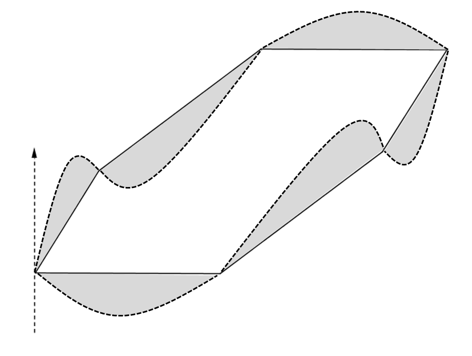
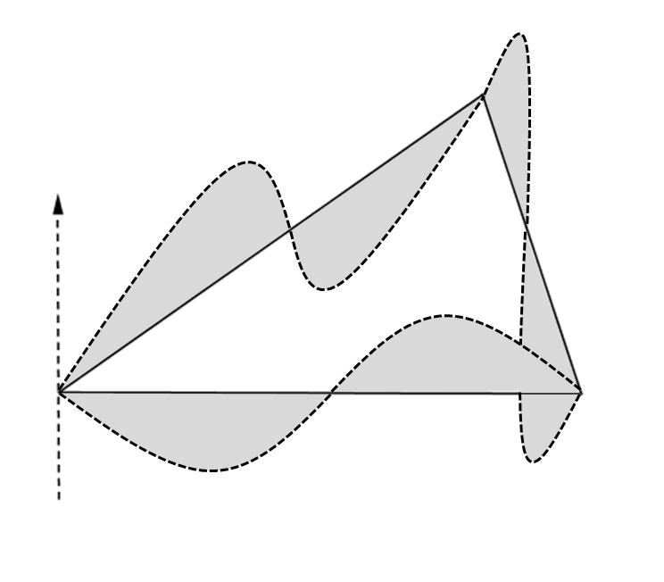
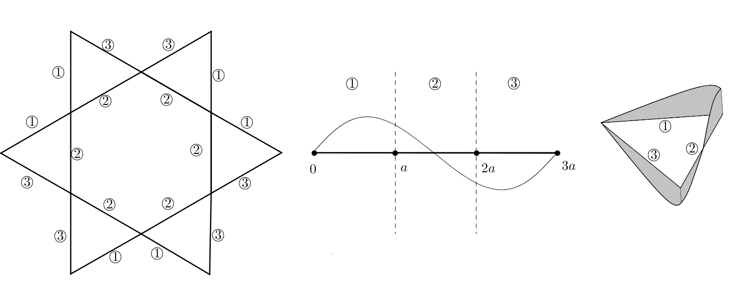
Similar as the case of hexagonal tiling [13, 11], the equation S⁡(a,ρ)=0S(a,\rho)=0 defines a point spectrum with infinite number of eigenfunctions. A typical example of these eigenfunctions is a repetition of the function φ2\varphi_{2} for the Dirichlet-Dirichlet boundary conditions around any basic triangular unit, while vanishing elsewhere. Another example is a repetition of φ1\varphi_{1} around any basic hexagonal unit. There are infinite number of such eigenfunctions on the periodic quantum graph. Besides the two examples as the following shaded functions on a hexagon (type (a) or a triangle (type (b), extended by zero to the rest of the graph, another class of eigenfunctions (type (c)) are also found (see Fig. 5).

Refer to caption
(a)
Refer to caption
(b)
Refer to caption
(c)
Figure 5: Eigenfunctions for trihexagonal tiling

Let us explain the class of type (c) eigenfunctions. By the theory of Hill’s discriminant [5, Theorem 2.3.1], the condition S′(a,ρ)=−1/2S^{\prime}(a,\rho)=-1/2 defines a sequence of eigenpairs (λn,un)(\lambda_{n},u_{n}) on the interval [0,a][0,a]. This sequence of solutions unu_{n}, if extended, has nn periods in (0,3​a)(0,3a). The graphs, on each subintervals are different, and are names as graphs ①,②,③\textcircled{1},\textcircled{2},\textcircled{3}. They represent Dirichlet-Dirchlet eigenfunctions on [0,3​a][0,3a] because from Theorem 1.3 (a),(b) and (d), with λn=ρn2\lambda_{n}=\rho_{n}^{2},

S′​(2​a,ρn)\displaystyle S^{\prime}(2a,\rho_{n}) =\displaystyle= C⁡(2​a,ρn)=2​S′​(a,ρn)2−1=−12;\displaystyle C(2a,\rho_{n})=2\,S^{\prime}(a,\rho_{n})^{2}-1=-\frac{1}{2};
S⁡(2​a,ρn)\displaystyle S(2a,\rho_{n}) =\displaystyle= 2​S​(a,ρn)​S′​(a,ρn)=−S⁡(a,ρn).\displaystyle 2\,S(a,\rho_{n})S^{\prime}(a,\rho_{n})=-S(a,\rho_{n}).

Notice that if we fold the graph to base it on a triangle with sidelength aa, and place six of them on the sides of a hexagon, allowing the function to vanish on the rest of the graph (see Fig. 5), we obtain a sequence of eigenfunctions for the quantum graph with eigenvalues λn\lambda_{n}’s. The multiplicity for each eigenvalue λn\lambda_{n} is infinite.

6 More analysis on the spectrum

In this section, we study the spectra of these periodic quantum graphs in more detail. In short, we try to understand more about the point spectrum σp\sigma_{p} and the asymptotic behavior of the absolutely continuous spectrum σa​c\sigma_{ac}. Define ℕk={1,2,…,k}\mathbb{N}_{k}=\{1,2,\ldots,k\}, for any k∈ℕk\in\mathbb{N}.

Theorem 6.1.
  1. (a)

    The point spectrum of the periodic quantum graph associated with triangular tiling satisfies

    σp​(HT)=⋃i,j∈ℕ3{ρ2∈ℝ:Si​(a,ρ)=Sj​(a,ρ)=0}\sigma_{p}(H_{T})=\bigcup_{i,j\in\mathbb{N}_{3}}\{\rho^{2}\in\mathbb{R}:\ S_{i}(a,\rho)=S_{j}(a,\rho)=0\}
  2. (b)

    The point spectrum of the periodic quantum graph associated with elongated triangular tiling satisfies

    σp​(He​T)=⋃i,j,k∈ℕ5{ρ2∈ℝ:Si​(a,ρ)=Sj​(a,ρ)=Sk​(a,ρ)=0}\sigma_{p}(H_{eT})=\bigcup_{i,j,k\in\mathbb{N}_{5}}\{\rho^{2}\in\mathbb{R}:\ S_{i}(a,\rho)=S_{j}(a,\rho)=S_{k}(a,\rho)=0\}
  3. (c)

    The point spectrum of the periodic quantum graph associated with truncated square tiling satisfies: λ=ρ2\lambda=\rho^{2} lies in σp​(Ht​r​S)\sigma_{p}(H_{trS}) if and only if ρ\rho satisfies

    2​S1​S3\displaystyle 2S_{1}S_{3} =\displaystyle= 2​S2​S4=C6​S1​S2+S6​(S1​S2)′+(S3​S4​S6)′\displaystyle 2S_{2}S_{4}\ =\ C_{6}S_{1}S_{2}+S_{6}(S_{1}S_{2})^{\prime}+(S_{3}S_{4}S_{6})^{\prime} (6.1)
    =\displaystyle= S5′​S2​S3+S5​(C​S)23+(C​S​S)145= 0,\displaystyle S_{5}^{\prime}S_{2}S_{3}+S_{5}(CS)_{23}+(CSS)_{145}\ =\ 0\ ,

    and

    0\displaystyle 0 =\displaystyle= (C​S​S)145​(S2′​(C3​S6)′+C2′​(S3​S6)′+C6​(C​S)23′−C1′​(S4​S6)′−S1′​(C4​S6)′−S1​(C4​C6)′CLOSE\displaystyle(CSS)_{145}\,\left(S_{2}^{\prime}(C_{3}S_{6})^{\prime}+C_{2}^{\prime}(S_{3}S_{6})^{\prime}+C_{6}(CS)_{23^{\prime}}-C_{1}^{\prime}(S_{4}S_{6})^{\prime}-S_{1}^{\prime}(C_{4}S_{6})^{\prime}-S_{1}(C_{4}C_{6})^{\prime}\right. (6.2)
    OPEN−C1​(S4​C6)′)+(S3​S4​S6)′​(C1​S2′​S5′+S1′​C2​C5−C5′​(S3​S4)′−C3​S4′​C5−S3′​C4​S5′)\displaystyle\left.-C_{1}(S_{4}C_{6})^{\prime}\right)+(S_{3}S_{4}S_{6})^{\prime}\,\left(C_{1}S_{2}^{\prime}S_{5}^{\prime}+S_{1}^{\prime}C_{2}C_{5}-C_{5}^{\prime}(S_{3}S_{4})^{\prime}-C_{3}S_{4}^{\prime}C_{5}-S_{3}^{\prime}C_{4}S_{5}^{\prime}\right)
    +S5​S6​((C​S)14′​(C​S)32′+(C​S)41′​(C​S)23′−2)\displaystyle+S_{5}S_{6}\,\left((CS)_{14^{\prime}}\,(CS)_{32^{\prime}}+(CS)_{41^{\prime}}\,(CS)_{23^{\prime}}-2\right)
  4. (d)

    The point spectrum of the periodic quantum graph associated with trihexagonal tiling satisfies: λ=ρ2\lambda=\rho^{2} lies in σp​(HT​H)\sigma_{p}(H_{TH}) if and only if ρ\rho satisfies

    0\displaystyle 0 =\displaystyle= S1​S3​S5+S2​S4​S6+(C​S​S​S)1346=S1​S4​S5+S2​S3​S6+(S2​S3​S4​S5)′\displaystyle S_{1}S_{3}S_{5}+S_{2}S_{4}S_{6}+(CSSS)_{1346}=S_{1}S_{4}S_{5}+S_{2}S_{3}S_{6}+(S_{2}S_{3}S_{4}S_{5})^{\prime} (6.3)
    =\displaystyle= S1​S2​S4+S3​S5​S6+S1​S6​(C​S)25+S2​S5​(S1​S6)′\displaystyle S_{1}S_{2}S_{4}+S_{3}S_{5}S_{6}+S_{1}S_{6}\,(CS)_{25}+S_{2}S_{5}\,(S_{1}S_{6})^{\prime}

    and

    0\displaystyle 0 =\displaystyle= −S1​S2​S3−S4​S5​S6+(S1​S3​S5+S2​S4​S6)​((C​S)16)′+(S1​S4​S5+S2​S6​S6)​((C​S)25)′\displaystyle-S_{1}S_{2}S_{3}-S_{4}S_{5}S_{6}+(S_{1}S_{3}S_{5}+S_{2}S_{4}S_{6})\,((CS)_{16})^{\prime}+(S_{1}S_{4}S_{5}+S_{2}S_{6}S_{6})\,((CS)_{25})^{\prime}
    +(S1​S2​S4+S3​S5​S6)​((C​S)34)′+(S1​S6)′​(S2​S5)′​(C​S)34+(S3​S4)′​(C​S)25​(C​S)16.\displaystyle+(S_{1}S_{2}S_{4}+S_{3}S_{5}S_{6})\,((CS)_{34})^{\prime}+(S_{1}S_{6})^{\prime}\,(S_{2}S_{5})^{\prime}\,(CS)_{34}+(S_{3}S_{4})^{\prime}\,(CS)_{25}\,(CS)_{16}.

Remark. It is easy to verify that for the spectrum σ⁡(Ht​r​S){\sigma(H_{trS})} related to truncated square tiling,

⋃i,j,k,l,m∈ℕ6{ρ2∈ℝ:Si=Sj=Sk=Sl=Sm=0}⊆σp​(Ht​r​S).\bigcup_{i,j,k,l,m\in\mathbb{N}_{6}}\{\rho^{2}\in\mathbb{R}:\ S_{i}=S_{j}=S_{k}=S_{l}=S_{m}=0\}\ \subseteq\ \sigma_{p}(H_{trS})\ .

In particular, σp​(Ht​r​S)\sigma_{p}(H_{trS}) contains those ρ\rho which satisfies S1=S2=S3=S4=S5=S6=0S_{1}=S_{2}=S_{3}=S_{4}=S_{5}=S_{6}=0, whence the eigenfunction is known and there are infinitely many of them. Then for the spectrum σp​(HT​H)\sigma_{p}(H_{TH}) related to trihexagonal tiling,

⋃i,j,k,l∈ℕ6{ρ2∈ℝ:Si=Sj=Sk=Sl=0}⊆σp​(HT​H).\bigcup_{i,j,k,l\in\mathbb{N}_{6}}\{\rho^{2}\in\mathbb{R}:\ S_{i}=S_{j}=S_{k}=S_{l}=0\}\ \subseteq\ {\sigma_{p}(H_{TH})}\ .

Certainly it includes the case when all SiS_{i}’s are zero.

Proof.

(a) For the triangular tiling, let

ψ(ρ,θ1,θ2)=(S1S2S3)′+(CSS)123−2S1S2cos(θ2−θ1)−2S2S3cosθ1−2S1S3cosθ2.\psi(\rho,\theta_{1},\theta_{2})=(S_{1}S_{2}S_{3})^{\prime}+(CSS)_{123}-2S_{1}S_{2}\,\cos(\theta_{2}-\theta_{1})-2S_{2}S_{3}\,\cos\theta_{1}-2S_{1}S_{3}\,\cos\theta_{2}. (6.5)

Now by the characterization of point spectrum, σp​(HT)\sigma_{p}(H_{T}) contains exactly those λ=ρ2\lambda=\rho^{2} which do not vary with Θ\Theta. Hence for any θ1,θ2∈[−π,π]\theta_{1},\theta_{2}\in[-\pi,\pi], from Theorem 2.1,

0\displaystyle 0 =\displaystyle= ∂ψ∂θ1=2S1S2sin(θ2−θ1)+2S2S3sinθ1\displaystyle\frac{\partial\psi}{\partial\theta_{1}}=2S_{1}S_{2}\,\sin(\theta_{2}-\theta_{1})+2S_{2}S_{3}\,\sin\theta_{1}
0\displaystyle 0 =\displaystyle= ∂ψ∂θ2=−2S1S2sin(θ2−θ1)+2S2S3sinθ2\displaystyle\frac{\partial\psi}{\partial\theta_{2}}=-2S_{1}S_{2}\,\sin(\theta_{2}-\theta_{1})+2S_{2}S_{3}\,\sin\theta_{2}

Hence either S2=0S_{2}=0 or S1=S3=0S_{1}=S_{3}=0. In the first case, (6.5) implies

S1S3(S2′+C2−2cosθ2)=0,S_{1}S_{3}\,(S_{2}^{\prime}+C_{2}-2\cos\theta_{2})=0,

which means that either S1=0S_{1}=0 or S3=0S_{3}=0. Thus part (a) is proved.
(b) For the elongated triangular tiling, for any θ1,θ2\theta_{1},\theta_{2}, from Theorem 3.1,

∂ψ∂θ1\displaystyle\frac{\partial\psi}{\partial\theta_{1}} =\displaystyle= 2((S1S2S3S4)′+(CSSS)1345+S1S2S5+S1S3S4(C2+S5′+8cosθ1))sinθ1\displaystyle 2\left((S_{1}S_{2}S_{3}S_{4})^{\prime}+(CSSS)_{1345}+S_{1}S_{2}S_{5}+S_{1}S_{3}S_{4}(C_{2}+S_{5}^{\prime}+8\cos\theta_{1})\right)\,\sin\theta_{1} (6.6)
+2​S2​S3​S5​sin⁡(θ1−θ2)= 0\displaystyle+2S_{2}S_{3}S_{5}\,\sin(\theta_{1}-\theta_{2})\ =\ 0
∂ψ∂θ2\displaystyle\frac{\partial\psi}{\partial\theta_{2}} =\displaystyle= 2S2S4S5sinθ2−2S2S3S5sin(θ1−θ2)= 0.\displaystyle 2S_{2}S_{4}S_{5}\,\sin\theta_{2}-2S_{2}S_{3}S_{5}\,\sin(\theta_{1}-\theta_{2})\ =\ 0. (6.7)

The equation (6.7) implies S2​S5=0S_{2}S_{5}=0, or S3=S4=0S_{3}=S_{4}=0, while S1​S3​S4=0S_{1}S_{3}S_{4}=0 follows from the first case. Eventually, we have that in any case there exists i,j,k∈ℕ5i,j,k\in\mathbb{N}_{5} such that Si=Sj=Sk=0S_{i}=S_{j}=S_{k}=0.
(c) For truncated square tiling, when θ1,θ2∈[−π,π]\theta_{1},\theta_{2}\in[-\pi,\pi], from Theorem 4.1 with ψ=Φ⁡(ρ)​e−i⁡(θ1+θ2)\displaystyle\psi=\Phi(\rho)\,{\rm e}^{-i(\theta_{1}+\theta_{2})},

∂ψ∂θ1\displaystyle\frac{\partial\psi}{\partial\theta_{1}} =\displaystyle= 2(C6S1S2+S6(S1S2)′+(S3S4S6)′)sinθ1\displaystyle 2\left(C_{6}S_{1}S_{2}+S_{6}(S_{1}S_{2})^{\prime}+(S_{3}S_{4}S_{6})^{\prime}\right)\,\sin\theta_{1}
+2​S2​S4​sin⁡(θ1−θ2)+2​S1​S3​sin⁡(θ1+θ2)= 0\displaystyle+2S_{2}S_{4}\,\sin(\theta_{1}-\theta_{2})+2S_{1}S_{3}\,\sin(\theta_{1}+\theta_{2})\ =\ 0
∂ψ∂θ2\displaystyle\frac{\partial\psi}{\partial\theta_{2}} =\displaystyle= 2(S5′S2S3+S5(CS)23+(CSS)145)sinθ2\displaystyle 2\left(S_{5}^{\prime}S_{2}S_{3}+S_{5}(CS)_{23}+(CSS)_{145}\right)\,\sin\theta_{2}
−2​S2​S4​sin⁡(θ1−θ2)+2​S1​S3​sin⁡(θ1+θ2)= 0.\displaystyle-2S_{2}S_{4}\,\sin(\theta_{1}-\theta_{2})+2S_{1}S_{3}\,\sin(\theta_{1}+\theta_{2})\ =\ 0.

It follows that (6.1) is valid. Together with Theorem 4.1, (6.2) also follows.
(d) For trihexagonal tiling, from Theorem 5.1,

∂ψ∂θ1\displaystyle\frac{\partial\psi}{\partial\theta_{1}} =\displaystyle= −2(S1S2S4+S3S5S6+S1S6(CS)25+S2S5(S1S6)′)sinθ1\displaystyle-2\left(S_{1}S_{2}S_{4}+S_{3}S_{5}S_{6}+S_{1}S_{6}(CS)_{25}+S_{2}S_{5}(S_{1}S_{6})^{\prime}\right)\,\sin\theta_{1}
−(S1​S3​S5+S2​S4​S6+(C​S​S​S)1346)​sin⁡(θ1−θ2)= 0\displaystyle-(S_{1}S_{3}S_{5}+S_{2}S_{4}S_{6}+(CSSS)_{1346})\,\sin(\theta_{1}-\theta_{2})\ =\ 0
∂ψ∂θ2\displaystyle\frac{\partial\psi}{\partial\theta_{2}} =\displaystyle= −2(S1S4S5+S2S3S6+(S2S3S4S5)′)sinθ2\displaystyle-2(S_{1}S_{4}S_{5}+S_{2}S_{3}S_{6}+(S_{2}S_{3}S_{4}S_{5})^{\prime})\,\sin\theta_{2}
+(S1​S3​S5+S2​S4​S6+(C​S​S​S)1346)​sin⁡(θ1−θ2)= 0\displaystyle+(S_{1}S_{3}S_{5}+S_{2}S_{4}S_{{6}}+(CSSS)_{1346})\,\sin(\theta_{1}-\theta_{2})\ =\ 0

These implies (6.3), and together with Theorem 5.1 also yields (). ∎

The explicit dispersion relations given in Theorem 1.1, assuming all qiq_{i}’s are identical and even, are simpler. They are all of the form Si​p​(S′)=0{S^{i}\,p(S^{\prime})=0}, where pp is a polynomial whose coefficients depend on θ1\theta_{1} and θ2\theta_{2}. Clearly, the point spectrum is defined by S=0S=0, while the polynomials in S′S^{\prime} define the absolutely continuous spectra.
Proof of Theorem 1.2:
For the triangular tiling, the dispersion relation (1.2) implies ρ2∈σa​c​(HT)\rho^{2}\in\sigma_{ac}(H_{T}) if and only if

S′​(a,ρ)=43​cos⁡θ12​cos⁡θ22​cos⁡θ1−θ22−13=16​|1+ei​θ1+ei​θ2|2−12,S^{\prime}(a,\rho)=\frac{4}{3}\cos\frac{\theta_{1}}{2}\cos\frac{\theta_{2}}{2}\cos\frac{\theta_{1}-\theta_{2}}{2}-\frac{1}{3}=\frac{1}{6}\,\left|1+{\rm e}^{i\theta_{1}}+{\rm e}^{i\theta_{2}}\right|^{2}-\frac{1}{2},

by (1.6). Since the range of |1+ei​θ1+ei​θ2|\displaystyle\left|1+{\rm e}^{i\theta_{1}}+{\rm e}^{i\theta_{2}}\right| is [0,3][0,3]. We conclude that ρ2∈σa​c​(HT)\rho^{2}\in\sigma_{ac}(H_{T}) if and only if

S′​(a,ρ)∈[−12,1].S^{\prime}(a,\rho)\in[-\frac{1}{2},1].

In the case of elongated triangular tiling, the dispersion relation (1.3) is

(S′)2−(45cosθ1)S′−125(8cosθ12cosθ22cosθ1−θ22−4cos2θ1+1)=0.(S^{\prime})^{2}-(\frac{4}{5}\cos\theta_{1})\,S^{\prime}-\frac{1}{25}\left(8\cos\frac{\theta_{1}}{2}\cos\frac{\theta_{2}}{2}\cos\frac{\theta_{1}-\theta_{2}}{2}-4\cos^{2}\theta_{1}+1\right)=0.

It implies, through (1.6), that ρ2∈σa​c​(He​T)\rho^{2}\in\sigma_{ac}(H_{eT}) iff

S′(a,ρ)=25cosθ1±15|1+ei​θ1+ei​θ2|∈[−35,1].S^{\prime}(a,\rho)=\frac{2}{5}\cos\theta_{1}\pm\frac{1}{5}\left|1+{\rm e}^{i\theta_{1}}+{\rm e}^{i\theta_{2}}\right|\in[-\frac{3}{5},1].

For truncated square tiling, if we let θ1=θ2=θ\theta_{1}=\theta_{2}=\theta, then (1.4) implies

0\displaystyle 0 =\displaystyle= (9​S′2−1)2−(36​S′2+24​cos⁡θ​S′+4​cos2⁡θ)\displaystyle(9S^{\prime 2}-1)^{2}-(36S^{\prime 2}+24\cos\theta\,S^{\prime}+4\,\cos^{2}\theta)
=\displaystyle= (9​S′2−1−6​S′−2​cos⁡θ)​(9​S′2−1+6​S′+2​cos⁡θ).\displaystyle(9S^{\prime 2}-1-6S^{\prime}-2\cos\theta)(9S^{\prime 2}-1+6S^{\prime}+2\cos\theta).

Thus,

S′​(a,ρ)=13​(1±2​cos⁡θ2)∈[13,1]∪[−13,13]=[−13,1];S^{\prime}(a,\rho)=\frac{1}{3}({1\pm 2\cos\frac{\theta}{2}})\in[\frac{1}{3},1]\cup[-\frac{1}{3},\frac{1}{3}]=[-\frac{1}{3},1];

or

S′​(a,ρ)=13​(−1±2​sin⁡θ2)∈[−1,−13]∪[−13,13]=[−1,13].S^{\prime}(a,\rho)=\frac{1}{3}({-1\pm 2\sin\frac{\theta}{2}})\in[-1,-\frac{1}{3}]\cup[-\frac{1}{3},\frac{1}{3}]=[-1,\frac{1}{3}].

Also, if |S′​(a,ρ)|=1+ϵ|S^{\prime}(a,\rho)|=1+\epsilon with ϵ>0\epsilon>0, then

(9​S′2−1)2−4​(3​S′+cos⁡θ1)​(3​S′+cos⁡θ2)≥192​ϵ+432​ϵ2+324​ϵ3+81​ϵ4>0.(9S^{\prime 2}-1)^{2}-4(3S^{\prime}+\cos\theta_{1})(3S^{\prime}+\cos\theta_{2})\geq 192\epsilon+432\epsilon^{2}+324\epsilon^{3}+81\epsilon^{4}>0.

Hence we conclude that σa​c(Ht​r​S)={S′(a,ρ)∈[−1,1]}\displaystyle\sigma_{ac}(H_{trS})=\left\{S^{\prime}(a,\rho)\in\left[-1,1\right]\right\}.

Finally the dispersion relation (1.5) for trihexagonal tiling involves

2​S′2−S′−cos⁡(θ12)​cos⁡(θ12)​cos⁡(θ1−θ22)=0.2S^{\prime 2}-S^{\prime}-\cos(\frac{\theta_{1}}{2})\cos(\frac{\theta_{1}}{2})\cos(\frac{\theta_{1}-\theta_{2}}{2})=0.

This implies that ρ2∈σa​c​(HT​H)\rho^{2}\in\sigma_{ac}(H_{TH}) iff

S′\displaystyle S^{\prime} =\displaystyle= 1±1+8​cos⁡θ12​cos⁡θ22​cos⁡θ1−θ224\displaystyle\frac{1\pm\sqrt{1+8\cos\frac{\theta_{1}}{2}\cos\frac{\theta_{2}}{2}\cos\frac{\theta_{1}-\theta_{2}}{2}}}{4}
=\displaystyle= 14​(1±|1+ei​θ1+ei​θ2|)\displaystyle\frac{1}{4}(1\pm|1+{\rm e}^{i\theta_{1}}+{\rm e}^{i\theta_{2}}|)
∈\displaystyle\in [14,1]∪[−12,14]=[−12,1].\displaystyle{[\frac{1}{4},1]\cup[-\frac{1}{2},\frac{1}{4}]=[-\frac{1}{2},1]}.

□\Box

In case q=0q=0, then S′​(a,ρ)=cos⁡(ρ​a)S^{\prime}(a,\rho)=\cos(\rho a). Hence from above, we have the following

  1. (a)

    σa​c​(HT)=σa​c​(HT​H)=[0,4​π29​a2]∪⋃n=1∞[(2​n−23)2​π2a2,(2​n+23)2​π2a2]\displaystyle\sigma_{ac}(H_{T})=\sigma_{ac}(H_{TH})=\left[0,\frac{4\pi^{2}}{9a^{2}}\right]\cup\bigcup_{n=1}^{\infty}\left[(2n-\frac{2}{3})^{2}\frac{\pi^{2}}{a^{2}},\,(2n+\frac{2}{3})^{2}\frac{\pi^{2}}{a^{2}}\right]

  2. (b)

    σa​c​(He​T)=[0,(ηa)2]∪⋃n=1∞[(2​n​π−ηa)2,(2​n​π+ηa)2]\displaystyle\sigma_{ac}(H_{eT})=\left[0,\left(\frac{\eta}{a}\right)^{2}\right]\cup\bigcup_{n=1}^{\infty}\left[\left(\frac{2n\pi-\eta}{a}\right)^{2},\left(\frac{2n\pi+\eta}{a}\right)^{2}\right], η=cos−1⁡(−35)∼2.2143\eta=\cos^{-1}(-\frac{3}{5})\sim 2.2143

  3. (c)

    σa​c​(Ht​r​S)=ℝ\sigma_{ac}(H_{trS})=\mathbb{R}

7 Concluding remarks

Just like the case of trihexagonal tiling, we found infinitely many eigenfunctions for the point spectra for the periodic quantum graphs associated with the other three Archimedean tiling. Most eigenfunctions involves types (a) and (b) shown in Figure 3. They are based on one triangle or one square of the tiling, and there are infinitely many of them. But for trihexagonal tiling we also have additional eigenfunctions based on a hexagon; and for truncated square tiling we have similar eigenfunctions based on a octagon.

As a summary, we have proved that the dispersion relations for the periodic quantum graphs associated with the 4 Archimedean tilings are of the form Si​(2​S′−1)j​p​(S′)=0S^{i}(2S^{\prime}-1)^{j}p(S^{\prime})=0 for some i,j≥0i,j\geq 0, and polynomial pp. Also their absolutely continuous spectra satisfy σa​c⊂ϕ−1​([−1,1])\sigma_{ac}\subset\phi^{-1}([-1,1]) where ϕ⁡(ρ)=S′​(a,ρ)\phi(\rho)=S^{\prime}(a,\rho). The spectra are all of a band and gap structure. In a next paper [18], we shall see that the situation for the other Archimedean tiling are essentially the same. Their dispersion relations are of the form Si​(2​S′−1)j​(2​S′+1)k​p​(S′)=0S^{i}(2S^{\prime}-1)^{j}(2S^{\prime}+1)^{k}p(S^{\prime})=0, and their absolutely continuous spectra satisfy σa​c⊂ϕ−1​([−1,1])\sigma_{ac}\subset\phi^{-1}([-1,1]).

We would like to emphasize that the dispersion relations are derived with the help of Mathematica, because of the determinants of large matrices (12×1212\times 12 at the most). To guarantee that these relations are indeed correct, we also plug in arbitrary numerical values of Si​(a,ρ)S_{i}(a,\rho), Si′​(a,ρ)S^{\prime}_{i}(a,\rho) and Ci​(a,ρ)C_{i}(a,\rho) into the characteristic functions in Theorem 2.1-Theorem 5.1, to verify that they match with the determinants. Thus we are sure that our results are correct.

The dispersion relations obtained in this paper make it easy for the analysis of the spectrum. We believe that there will be a lot of interesting properties about these quantum graphs to be dug out. We also emphasize that our method, through some hard work, may allow qiq_{i}’s to be neither identical, nor even, as given in Theorems 2.1=5.1. For the sake of completeness, we also include the cases of square tiling [14],

(C1​S2​S3​S4)′+(S1​C2​S3​S4)′+(S1​S2​C3​S4)′+(S1​S2​S3​C4)′\displaystyle(C_{1}S_{2}S_{3}S_{4})^{\prime}+(S_{1}C_{2}S_{3}S_{4})^{\prime}+(S_{1}S_{2}C_{3}S_{4})^{\prime}+(S_{1}S_{2}S_{3}C_{4})^{\prime}
=\displaystyle= 2[(S1S3+S2S4)cosθ1+(S1S2+S3S4)cosθ2+S2S3cos(θ1+θ2)+S1S4cos(θ1−θ2)].\displaystyle 2[(S_{1}S_{3}+S_{2}S_{4})\cos\theta_{1}+(S_{1}S_{2}+S_{3}S_{4})\cos\theta_{2}+S_{2}S_{3}\cos(\theta_{1}+\theta_{2})+S_{1}S_{4}\cos(\theta_{1}-\theta_{2})].

Acknowledgements

The authors are grateful to the anonymous reviewers for their very careful reading and constructive comments. Their suggestions help us to improve the paper significantly and correct some mistakes. We also thank Vyacheslav Pivovarchik and Min-Jei Huang for stimulating discussions. The authors are partially supported by Ministry of Science and Technology, Taiwan, under contract number MOST105-2115-M-110-004.

Table 1: Table of 11 Archimedean tilings

NameTriangular tilingSnub trihexagonal tilingElongated triangular tilingNotation(36)(34,6)(33,42)[Uncaptioned image][Uncaptioned image][Uncaptioned image]NameSnub square tilingTrihexagonal tilingRhombi-trihexagonal tilingNotation(32,4,3,4)(3,6,3,6)(3,4,6,4)[Uncaptioned image][Uncaptioned image][Uncaptioned image]NameTruncated hexagonal tilingSquare tilingTruncated trihexagonal tilingNotation(3,122)(44)(4,6,12)[Uncaptioned image][Uncaptioned image][Uncaptioned image]NameTruncated square tilingHexagonal tilingNotation(4,82)(63)[Uncaptioned image][Uncaptioned image]\begin{array}[]{|c||c|c|c|}\hline\cr\text{Name}&\text{Triangular tiling}&\text{{\small Snub trihexagonal tiling}}&\text{{\small Elongated triangular tiling}}\\ \hline\cr\text{Notation}&\left(3^{6}\right)&\left(3^{4},6\right)&\left(3^{3},4^{2}\right)\\ \hline\cr&\includegraphics[width=85.35826pt]{A01.png}&\includegraphics[width=85.35826pt]{A02.png}&\includegraphics[width=85.35826pt]{A03.png}\\ \hline\cr\hline\cr\text{Name}&\text{Snub square tiling}&\text{Trihexagonal tiling}&\text{{\small Rhombi-trihexagonal tiling}}\\ \hline\cr\text{Notation}&\left(3^{2},4,3,4\right)&(3,6,3,6)&(3,4,6,4)\\ \hline\cr&\includegraphics[width=85.35826pt]{A04.png}&\includegraphics[width=85.35826pt]{A05.png}&\includegraphics[width=85.35826pt]{A06.png}\\ \hline\cr\hline\cr\text{Name}&\text{{\small Truncated hexagonal tiling}}&\text{Square tiling}&\text{{\small Truncated trihexagonal tiling}}\\ \hline\cr\text{Notation}&\left(3,12^{2}\right)&\left(4^{4}\right)&(4,6,12)\\ \hline\cr&\includegraphics[width=85.35826pt]{A07.png}&\includegraphics[width=85.35826pt]{A08.png}&\includegraphics[width=85.35826pt]{A09.png}\\ \hline\cr\hline\cr\text{Name}&\text{{\small Truncated square tiling}}&\text{Hexagonal tiling}&\\ \hline\cr\text{Notation}&\left(4,8^{2}\right)&(6^{3})&\\ \hline\cr&\includegraphics[width=85.35826pt]{A10.png}&\includegraphics[width=85.35826pt]{A11.png}&\\ \hline\cr\end{array}

References

  • [1] C. Amovilli, F.E. Leys, and N.H. March, Electronic energy spectrum of two-Dimensional solids and a chain of C atoms from a quantum network model, J. Math. Chem., 36 (2004), 93-112.
  • [2] G. Berkolaiko and A. Comech, Symmetry and Dirac points in graphene spectrum, J. Spectral Theory, 8 (2018) no.3, 1099-1147.
  • [3] G. Berkolaiko and P. Kuchment, Introduction to Quantum Graphs, Amer. Math. Soc., Providence, 2012.
  • [4] N.T. Do and P. Kuchment, Quantum graph spectra of a graphyne structure, Math. Quantum Nano Tech., 2 (2013) 107-123.
  • [5] M. Eastham, The Spectral Theory of Periodic Differential Equations, Scottish Academiac Press, Edinburgh and London, 1973.
  • [6] A. Enyanshin and A. Ivanovskii, Graphen alloptropes: stability, structural and electronic properties from DF-TB calculations, Phys. Status Solidi (b), 248 (2011) 1879-1883.
  • [7] P. Exner, J.P. Keating, P. Kuchment, T. Sunada and A. Teplyaev, Analysis on Graphs and Its Applications, Proceedings of a Isaac Newton Institute programme, Janunary 8-June 29, 2007, Proc. Symp. Pure Math. 77, American Mathematical Society, R. I., 2008.
  • [8] C.L. Fefferman and M.I. Weinstein, Honeycomb lattice potentials and Dirac points, J. Amer. Math. Soc. 25, (2012) 1169-1220.
  • [9] A. Geim, Nobel lecture: Random valk to graphene, Rev. Mod. Phys., 83 (2011) 851-862.
  • [10] B. Grünbaum and G. Shephard, Tilings and Patterns, W. H. Freeman and Company, New York, 1987.
  • [11] E. Korotyaev and I. Lobanov, Schrödinger operators on zigzag nanotubes, Ann. Henri Poincaré, 8 (2007), 1151-1176.
  • [12] P. Kuchment, Floquet Theory for Partial Differential Equations, Birkhäuse Verlag, Basel, (1993).
  • [13] P. Kuchment and O. Post, On the spectra of carbon nano-structures, Comm. Math. Phys., 275 (2007), 805-826.
  • [14] C.K. Law, Y.C. Luo and T.E. Wang, Periodic spectrum of nn-cubic quantum graphs, submitted (2018).
  • [15] C.K. Law and V. Pivovarchik, Characteristic functions of quantum graphs, J. Phys. A, 42 (2009), 12 pp.
  • [16] C.K. Law and E. Yanagida, A solution to an Ambarzumyan problem on trees, Kodai Math. J., 35 (2012), 358-373
  • [17] F.E. Leys, C. Amovilli and N.H. March, Topology, connectivity, and electronic structure of C and B cages and the corresponding nanotubes, J. Chem. Inf. Comput. Sci., 44 (2004), 122-135.
  • [18] Y.C. Luo, E.O. Jatulan and C.K. Law, Dispersion relations of periodic quantum graphs associated with Archimedean tilings (II), preprint (2018).
  • [19] W. Magnus and S. Winkler, Hill’s equation, 2nd ed., Dover, N.Y., 1979.
  • [20] K. Novoselov, Nobel lecture: Graphene: Materials in the flatland, Rev. Mod. Phys., 83 (2011) 837-849.
  • [21] V. Pivovarchik and N. Rozhenko, Inverse Sturm-Liouville proble on equilateral regular tree, Appl. Anal. , 92 (2013), 784-798.
  • [22] M. Reed and B. Simon, Methods of Modern Mathematical Physics IV: Analysis of Operators, Academic Press, New York, (1978).
  • [23] B. Simon, On the genericity of nonvanishing instability intervals in Hill’s equation, Ann. Inst. Henri Poincaré 24(1) (1976), 91-93.