Analysis of Outage Probabilities for Cooperative NOMA Users with Imperfect CSI
Abstract
Non-orthogonal multiple access (NOMA) is a promising spectrally-efficient technology to meet the massive data requirement of the next-generation wireless communication networks. In this paper, we consider a cooperative non-orthogonal multiple access (CNOMA) networks consisting of a base station and two users, where the near user serves as a decode-and-forward relay to help the far user, and investigate the outage probability of the CNOMA users under two different types of channel estimation errors. For both CNOMA users, we derive the closed-form expressions of the outage probability and discuss the asymptotic characteristics for the outage probability in the high signal-to-noise ratio (SNR) regimes. Our results show that for the case of constant variance of the channel estimation error, the outage probability of two users are limited by a performance bottleneck which related to the value of the error variance. In contrast, there is no such performance bottleneck for the outage probability when the variance of the channel estimation error deceases with SNR, and in this case the diversity gain is fully achieved by the far user.
Index Terms:
Outage probability, cooperative non-orthogonal multiple access, channel estimation error, decode-and-forward.I Introduction
Non-orthogonal multiple access (NOMA) has been considered as an emerging technology which can address the massive data requirement due to increasing demand of mobile Internet and the Internet-of-Things (IoT) for the fifth-generation (5G) wireless communications[1, 2]. Different from the conventional orthogonal multiple access (OMA) schemes, NOMA can accommodate substantially more users via non-orthogonal resource allocation to obtain a significant gain in spectral efficiency [3, 4, 5]. As an essential technology of 5G to achieve higher spectral efficiency and massive connectivity, NOMA was extended to cooperative transmission to enhance the transmission reliability for the users with poor channel conditions [6, 7]. Specifically, two types of cooperative NOMA (CNOMA) systems were introduced and classified by different cooperation schemes: the cooperation among the NOMA users [6, 8], and the CNOMA systems employing dedicated relays [7, 9]. It is shown that the above two types of CNOMA can utilize the resources of the network efficiently and improve the spectral efficiency of the system compared to cooperative OMA systems[10].
As perfect channel state information (CSI) cannot be acquired in practice due to the limited overhead of pilot signals in time-division-duplex systems and the finite capacity of feedback channel in frequency-division-duplex systems, the impact of imperfect CSI on NOMA networks has drawn much attention in recent years. Some early work addressed NOMA networks based on statistical characteristics of channels. For instance, the outage performance of a NOMA system was discussed in [11] with the priori knowledge of the distribution characteristics of the users’s location and their small scale fading. In [12], the ergodic capacity maximization problem was studied for the multiple-input multiple-output (MIMO) NOMA systems with statistical CSI acquired by the transmitters. Afterwards, the impact of channel estimation error was further discussed for practical systems in the following works [13, 14, 15, 16]. For instance, the authors in [13] investigated the outage probability and the average rate for NOMA systems under channel estimation error, with comparison of the NOMA systems when only statistical CSI is known by the receivers. In [14], a tractable analysis on the outage probability was performed for a downlink NOMA system with imperfect CSI on account of estimation error and noise. Based on that, the user selection and power allocation were optimized. Moreover, the study of NOMA systems with imperfect CSI was extended to multi-users MIMO-NOMA systems in [15], in which the rate gain of system was indicated by applying NOMA scheme in MIMO systems. Besides, the authors in [16] proposed a dynamic-ordered self-interference cancellation (SIC) receiver for NOMA systems with the assumption of imperfect CSI, then the advantage of the proposed receiver was shown with comparison of traditional SIC receiver under the same situation of imperfect CSI.
Despite the aforementioned progress on the study of NOMA systems under imperfect CSI, the impact of imperfect CSI on CNOMA networks is rarely addressed.
To the best of the authors’ knowledge, most of the previous literatures on CNOMA networks assume that perfect CSI can be obtained at the receivers [6, 7, 8, 9], which is infeasible in practical systems. In this paper, we investigate the outage performance of a downlink CNOMA system under imperfect CSI, in which two different types of CSI estimation errors, constant and variable variance of CSI estimation errors are assumed. Our contribution includes two parts:
1) For the considered two-user CNOMA system under imperfect CSI, we firstly derive the exact closed-form expression of the outage probability for the near user.
However, the closed-form expression of outage probability of the far user is too complicated and mathematical intractable. Therefore we propose an analytical approximation for that, which is validated to be sufficiently close to the exact outage probability of the far user;
2) With the above analytical results for outage probability of both users, we analyze the asymptotic behaviors of the outage probability in the high SNR regimes, and compared them between two types of channel estimation errors with constant and variable variance.
We found that a performance floor exist for the outage probability of both users in the high SNR regimes when the error variance keeps constant.
On the contrary, the outage probability of both users will decrease with the SNR when the errors variance is reduced by the increase of SNR. Moreover, we prove that the diversity gain of the far user can be fully achieved in the case of the variable error variance.
Monte-Carlo simulations are provided to validate our analytical results.
Notations— In this paper, we denote the probability and the expectation value of a random event by and , respectively. denotes the absolute value of a complex-valued scalar.

II System Model
Consider a model of a downlink CNOMA system as shown in Fig. 1, including one BS and two users (UE1 and UE2), in which UE1 and UE2 directly communicate with the BS. However, UE2 is much far away from the BS than UE1 so that UE2 needs the help from UE1. Each node is equipped with a single-antenna and UE1 serves as a relay (for UE2) operating in HD mode. For this system, we model all the channels as independent Rayleigh fading, and represent the channels between the BS and the two users and the channel between the two users as , , and , respectively. Besides, we assume that the CSI are estimated imperfectly at the receivers, thus we have [13]
| (1) |
where denotes the estimated channel coefficient for with and denotes the channel estimation error with , for . In this paper, two types of the channel estimation error are considered. The first one is that decreases inversely proportional to the received SNR by a scaling factor [17], and the second is that keeps constant [13].
The transmission scheme of CNOMA consists of two consecutive time slots with equal length, as described in the follows.
During the first time slot, the BS broadcasts a superimposed signal, ,
to both users, where and are the desired signals for UE1 and UE2, respectively, with
.
We denote the transmit power for UE1 and UE2 as and , respectively, and denote the total transmit power for the BS as .
Therefore the received signals at the two users are expressed by
| (2) |
where denotes the complex additive white Gaussian noise (AWGN) at the UE, i.e., .
We assume without loss of generality and set according to the NOMA protocol described in [18].
During the second time slot,
UE1 serves as a DF relay by transmitting to UE2 after was successfully detected.
This means that there are two cases of the received signal at UE2 as follows.
Case 1: When was not detected by UE1 successfully, then cannot be sent by UE1 and the received signal at UE2 is as represented by (2).
Case 2: When was detected by UE1 successfully, then UE1 transmit to UE2, and the received signal at UE2 is expressed as
| (3) |
where denotes the AWGN at UE2, i.e., . Then, by using the maximum ratio combining (MRC), the received signals from both time slots at UE2 are combined with the MRC coefficients, and , which yields
| (4) |
Based on the considered model, we can express the received SINRs at UE1 as
| (5) | ||||
| (6) |
where and , respectively, denote the SINRs for detecting and in the SIC process at UE1.
Then, according to the two cases for the received signals at UE2, the SINR at UE2 (for decoding ) are shown as follows.
Case 1: The received signal at UE2 is in (2)
and the SINR at UE2 is represented by
| (7) |
Case 2: The received signal at UE2 is in (4), and by using the property of MRC, the SINR at UE2 is given by
| (8) |
III Outage Probabilities under imperfect CSI
In this section, we investigate the outage probability, which is an important performance metric of the considered CNOMA system. The outage probability of the CNOMA users are both derived in closed-form expressions. Furthermore, the asymptotic characteristics of outage performance of the CNOMA users are investigated for the high SNR regimes and the impact of different CSI estimation errors on the outage performance of the CNOMA users are discussed.
III-A Outage Probabilities for CNOMA Users
To begin with, we characterize the outage probability achieved by this two-phase CNOMA system. Denoting the SINR thresholds of data rate requirements of UE1 and UE2 as and , respectively, the definition of the outage probability of UE1 is expressed as
| (9) |
and that of UE2 is expressed as .
We denote and note that is a sufficient condition for this considered CNOMA system working normally (It can be easily proved that when ). Therefore we assume for the analysis of the outage probability in the rest of this paper.
Then, the outage probability of UE1 is shown in Theorem 1.
Theorem 1.
The outage probability of UE1 is given by
| (10) |
where , , and .
Proof.
See Appendix A. ∎
Besides, the overall outage probability of UE2 is decided by the actual results of the outage probability of UE2 in the two cases, which are shown in the following lemma.
Lemma 1.
The outage probability of UE2 in Case 1 is given by
| (11) |
with , and the outage probability of UE2 in Case 2 is given by (12) (at top of next page).
| (12) |
Proof.
See Appendix B. ∎
However, the results in (12) is too complicated and is difficult to be analyzed. Therefore by using the mean value of , , to replace with in (12), we obtain an approximation of (12) as shown in the following lemma.
Lemma 2.
An approximation of the outage probability of UE2 in Case 2 is given by
| (13) |
where with , , , .
Proof.
See Appendix C. ∎
With the conclusions of Lemmas 1–2, we finally obtain the overall outage probability of UE2 as follows.
Theorem 2.
The overall outage probability of UE2 is approximated by (14) (at top of next page)
| (14) |
with , , and , .
Proof.
See Appendix D. ∎
III-B Asymptotic characteristics for CNOMA users
Since we have obtained the analytical expressions of outage probability of the two users, we then carry on a further study on asymptotic characteristics of and in the high SNR regimes. In specific, assuming that and both grow to infinity while with a constant ratio of , the asymptotic characteristics of the outage probability of both users are discussed under two different CSI estimation error assumptions. The analytical results are shown in the following theorem.
Theorem 3.
When is a constant, i.e., , , the outage probability of the two users both approach performance floors in the high SNR regimes, which are given by
| (15) | ||||
| (16) |
| (17) |
with in (17) (at top of next page) and , .
Besides, when is inversely proportional to the received SNR, i.e., , , the outage probability of the two users are given by
| (18) | ||||
| (19) |
It can be easily proved from (15) and (16) that there are performance floors for the outage probability of both CNOMA users in the high SNR regimes when the CSI estimation error variance keeps constant. Meanwhile, we can observe that the performance floors are independent of the received SNRs, and the floors increase with the error variance. However, there is no such performance bottleneck in the case of variable variance of CSI estimation error, and it is indicated from (18) and (19) that the outage probability of the two users both decrease with the increase of SNR. Moreover, it can be proved from (19) that the diversity order for UE2 is , which means the diversity gain is fully acquired by UE2 under variable error variance.
Proof.
Depending on the different types of CSI estimation errors, we substitute or , respectively into (10) and omit the the small terms in them for . Then by skipping the details of simplification, we obtain (15) and (18) for UE1. In the sequel, we substitute or , respectively into (14), for . Then we apply the Taylor’s expansions on the logarithmic and exponential functions in them and omit the small terms for . Finally, we obtain (16) and (19) for UE2. ∎
IV Numerical Results
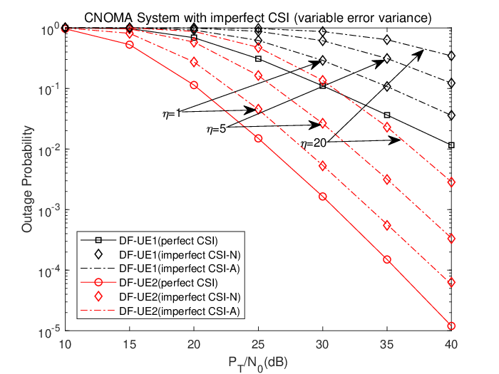

In this section, the outage probability of the CNOMA system is evaluated based on Monte-Carlo simulations averaging over independent channel realizations, considering different levels of channsl estimation error variances. Furthermore, the asymptotic characteristics of the outage probability of the users are shown in the high SNRs. The system performance with perfect CSI is also included as a benchmark. In specific, the adopted simulation system parameters are set as follows. The data requirements of UE1 and UE2 are set as bit/Hz/s and bit/Hz/s, respectively. The variances of channels fading for BS-UE1, BS-UE2, and UE1-UE2 are set as , , and , respectively. In addition, the power of noises are all set as , and the parameters of the transmit powers are set by and dB. In all the figures, the numerical results of outage probability are labeled ’-N’, and the analytical results of outage probability of UE1 (in (10)) and UE2 (in (14)) are labeled ’-A’. We set with and for the case of variable CSI estimation error variance, and set and for the case of constant CSI estimation error variance, for .
In Fig. 2, the outage probability of the two users under variable CSI estimation error variance are shown as a function of . An excellent agreement between the analytical and the Monte Carlo simulation results of outage probability of both users, which verifies the validity of the approximation for the outage probability of UE2. Compared with the CNOMA systems with perfect CSI, there is an increase of the outage probability of both users with imperfect CSI and the gap between them increases with . In addition, it is observed that the curves of the same user show the same slope degree (in log-scale) in the moderate-to-high SNR range, which indicates the outage performance with variable CSI estimation error variance can achieve the same diversity order with that of perfect CSI estimation, as been proved in Theorem 3.
Fig. 3 shows the variation of the outage probability of two CNOMA users under constant CSI estimation error variance, following the variation of . The analytical results of the outage probability of both users in Fig 3 show an excellent agreement with the Monte-Carlo simulation results of both users. It is also observed from Fig. 3 that there is an increase of the outage probability of both users with imperfect CSI in comparison with that with perfect CSI, while the gap between them increases with . Moreover, it is indicated from Fig. 3 that there is a floor for outage probability of both users under constant variance of CSI estimation error in high SNR regimes. This means that the constant variance of CSI estimation error causes a bottleneck of the outage performance in CNOMA systems, which validates the conclusion of Theorem 3.
V Conclusion
In this paper, we have studied the impact of imperfect CSI on the outage probability of downlink two-user CNOMA networks in which the near user acts as a DF relay for assisting the far user. For two different types of imperfect CSI estimation when the variance of the estimation error keeps constant value or decreases linearly with received SNR, the closed-form expressions of the outage probability of the two users were derived. Based on that, the asymptotic behaviors of the outage probability of both users were investigated. It is shown that the outage probability of both users under constant variance of errors approaches a performance bottleneck, even when the received SNRs are sufficiently high. Meanwhile, there is no such performance bottleneck for the outage probability of the two users when the error variance improves with the received SNRs. It is also shown that the diversity order of both users for the case of variable error variance are identical with that under perfect CSI.
Appendix A Proof of Theorem1
| (20) |
Appendix B Proof of Lemma 1
Firstly, we consider Case 1: When was not detected by UE1, the expression of is given by
| (24) |
and further recast into
| (25) |
We note that (25) has a similar form with (21), and it can be easily to obtain the expression of in (11).
Next, we consider Case 2: When was successfully detected by UE1 and then transmitted to UE2, the outage probability of UE2 is given by
| (26) |
with , .
With , , , the cumulative distribution function (CDF) of and the PDF of are given by (B) and (29) (at top of next page), respectively.
| (29) |
Appendix C Proof of Lemma 2
Firstly, the outage probability of UE2 is approximated by
| (30) |
with , , whilst the CDF of and the PDF of are given as follows.
Appendix D Proof of Theorem 2
Firstly, the approximation of the overall outage probability of UE2 is expressed as
| (34) |
where represents the probability of unsuccessfully decoding at UE1. Then, is recast into
| (35) |
Due to the similarity between (25) and (35), it can be easily obtained that
| (36) |
Then by substituting (36), (12) and (13) into (34) and through simplifications, we finally obtain in (14), which completes the proof.
Acknowledgment
The paper has been accepted by 2018 Information Technology and Mechatronics Engineering Conference (ITOEC 2018£©, 17th Sept. 2018.
References
- [1] M. Shirvanimoghaddam, M. Dohler, and S. J. Johnson, “Massive non-orthogonal multiple access for cellular IoT: Potentials and limitations,” IEEE Commun. Mag., vol. 55, no. 9, pp. 55–61, Sep. 2017.
- [2] V. W. S. Wong, R. Schober, D. W. K. Ng, and L.-C. Wang, Key Technologies for 5G Wireless Systems. Cambridge university press, 2017.
- [3] Y. Saito, Y. Kishiyama, A. Benjebbour, T. Nakamura, A. Li, and K. Higuchi, “Non-orthogonal multiple access (NOMA) for cellular future radio access,” in Proc. IEEE Vehicular Technology Conference (VTC), Dresden, Germany, Jun. 2013, pp. 1–5.
- [4] L. Dai, B. Wang, Y. Yuan, S. Han, C. l. I, and Z. Wang, “Non-orthogonal multiple access for 5G: solutions, challenges, opportunities, and future research trends,” IEEE Commun. Mag., vol. 53, no. 9, pp. 74–81, Sep. 2015.
- [5] S. M. R. Islam, N. Avazov, O. A. Dobre, and K. s. Kwak, “Power-domain non-orthogonal multiple access (NOMA) in 5G systems: Potentials and challenges,” IEEE Commun. Surveys Tuts., vol. 19, no. 2, pp. 721–742, Secondquarter 2017.
- [6] Z. Ding, M. Peng, and H. V. Poor, “Cooperative non-orthogonal multiple access in 5G systems,” IEEE Commun. Lett., vol. 19, no. 8, pp. 1462–1465, Aug. 2015.
- [7] J. B. Kim and I. H. Lee, “Non-orthogonal multiple access in coordinated direct and relay transmission,” IEEE Commun. Lett., vol. 19, no. 11, pp. 2037–2040, Nov. 2015.
- [8] Y. Zhou, V. W. S. Wong, and R. Schober, “Dynamic decode-and-forward based cooperative NOMA with spatially random users,” IEEE Trans. Wireless Commun., vol. 17, no. 5, pp. 3340–3356, May 2018.
- [9] X. Liang, Y. Wu, D. W. K. Ng, Y. Zuo, S. Jin, and H. Zhu, “Outage performance for cooperative NOMA transmission with an AF relay,” IEEE Commun. Lett., vol. 21, no. 11, pp. 2428–2431, Nov. 2017.
- [10] Z. Ding, X. Lei, G. K. Karagiannidis, R. Schober, J. Yuan, and V. K. Bhargava, “A survey on non-orthogonal multiple access for 5G networks: Research challenges and future trends,” IEEE J. Sel. Areas Commun., vol. 35, no. 10, pp. 2181–2195, Oct. 2017.
- [11] Z. Ding, Z. Yang, P. Fan, and H. V. Poor, “On the Performance of Non-Orthogonal Multiple Access in 5G Systems with Randomly Deployed Users,” IEEE Signal Process. Lett., vol. 21, no. 12, pp. 1501–1505, Dec. 2014.
- [12] Q. Sun, S. Han, C. L. I, and Z. Pan, “On the Ergodic Capacity of MIMO NOMA Systems,” IEEE Commun. Lett., vol. 4, no. 4, pp. 405–408, Aug. 2015.
- [13] Z. Yang, Z. Ding, P. Fan, and G. K. Karagiannidis, “On the performance of non-orthogonal multiple access systems with partial channel information,” IEEE Trans. Commun., vol. 64, no. 2, pp. 654–667, Feb. 2016.
- [14] W. Cai, C. Chen, L. Bai, Y. Jin, and J. Choi, “User Selection and Power Allocation Schemes for Downlink NOMA Systems with Imperfect CSI,” in Proc. IEEE Vehicular Technology Conference (VTC), Montreal, QC, Canada, Sep. 2016, pp. 1–5.
- [15] H. V. Cheng, E. Bjornson, and E. G. Larsson, “NOMA in multiuser MIMO systems with imperfect CSI,” in Proc. IEEE Workshop on Signal Processing Advances in Wireless Communications (SPAWC), Sapporo, Japan, Jul. 2017, pp. 1–5.
- [16] Y. Gao, B. Xia, Y. Liu, Y. Yao, K. Xiao, and G. Lu, “Analysis of the Dynamic Ordered Decoding for Uplink NOMA Systems with Imperfect CSI,” vol. 1, no. 1, pp. 1–1, Jan. 2018.
- [17] S. S. Ikki and S. Aissa, “Two-way amplify-and-forward relaying with gaussian imperfect channel estimations,” IEEE Commun. Lett., vol. 16, no. 7, pp. 956–959, Jul. 2012.
- [18] A. Benjebbour, Y. Saito, Y. Kishiyama, A. Li, A. Harada, and T. Nakamura, “Concept and practical considerations of non-orthogonal multiple access (NOMA) for future radio access,” in Proc. Intelligent Signal Processing and Communications Systems (ISPACS), Okinawa, Japan, Nov. 2013, pp. 770–774.