∎
Efimov states of three unequal bosons in non-integer dimensions Thanks: This work has been partially supported by the Spanish Ministerio de Economía y Competitividad under Project FIS2014-51971-P
Abstract
The Efimov effect for three bosons in three dimensions requires two infinitely large -wave scattering lengths. We assume two identical particles with very large scattering lengths interacting with a third particle. We use a novel mathematical technique where the centrifugal barrier contains an effective dimension parameter, which allows efficient calculations precisely as in ordinary three spatial dimensions. We investigate properties and occurrence conditions of Efimov states for such systems as functions of the third scattering length, the non-integer dimension parameter, mass ratio between unequal particles, and total angular momentum. We focus on the practical interest of the existence, number of Efimov states and their scaling properties. Decreasing the dimension parameter from towards the Efimov effect and states disappear for critical values of mass ratio, angular momentum and scattering length parameter. We investigate the relations between the four variables and extract details of where and how the states disappear. Finally, we supply a qualitative relation between the dimension parameter and an external field used to squeeze a genuine three dimensional system.
1 Introduction
The Efimov effect in three dimensions is characterized by a three-body system, where the two-body -wave scattering lengths for at least two of the three pairs are infinitely large, and consequently infinitely many bound three-body states can be found [1; 2]. This is a rigorous mathematical definition which can never be precisely obeyed, neither for systems found in nature nor for constructions in laboratories. Therefore it is essential to distinguish between occurrence conditions for the effect and appearance of a finite number of states that can be classified as Efimov states.
The Efimov effect has by now been demonstrated in many laboratories [3; 4; 5; 6], but only one direct measurement exists of an Efimov state [3]. All other observations are convincing but indirect and restricted to derived relative features of at most three different Efimov states. We shall therefore be concerned with the properties of only the lowest few Efimov states. This is already challenging as witnessed by the difficulties in laboratory tuning to the very well-known mathematical conditions.
The experimental techniques are crucial but fortunately very developed over the last decade. The decisive feature is tuning of the effective two-body interaction by use of the Feshbach resonance technique [7]. The central ingredient is the controllable external fields which are directly varied to place a two-body state at zero energy corresponding to infinite -wave scattering length. Clearly this tuning can only be approximate with a resulting finite scattering length.
The orders of the achievable control are such that cold atoms or molecules are the only candidates for this artificial tuning. On the other hand, then the technique is both efficient and flexible with external fields varying continuously from spherical to extremely deformed. This makes it practically possible to squeeze by use of a deformed external field, which effectively continuously reduces the spatial dimensions. The effects of this dimension variation has been investigated recently in various ways [8; 9; 10; 11].
A change of dimension from to is known to produce qualitative structure changes as evidenced by the fact that the Efimov effect exists in but not in [1]. Furthermore, the mass dependence and the dependence on the number (two or three) of contributing large scattering lengths are extremely important for scaling properties in [12], and in addition the third finite scattering length may have substantial effect [13]. Most likely then the variation with dimension would be crucial for these dependencies. In this report, we focus on the Efimov effect, and the number and structure of Efimov states as function of the dimension parameter, , varying between and .
In section II we first provide details of the theoretical formulation and section III describes the numerical procedure and pertinent basic properties. In section IV we discuss occurrence of the Efimov effect and provide characteristic properties of the corresponding states. In section V we discuss the meaning of the dimension parameter, and indicate an interpretation in terms of an external field. Finally, in section VI we conclude and point out some perspectives of this work.
2 Theoretical formulation
The Efimov effect is the appearance of an infinite number of bound states in a three-body system without bound two-body subsystems [14]. This occurs when at least two of the two-body -wave scattering lengths, and , are infinitely large. We shall focus on the third scattering length, , since the properties depend substantially on its value between and [13]. We shall first specify which systems to study, then define key quantities, give equations to determine them, and discuss schematic numerical results.

2.1 Specifying system and purpose
The system consists of three point-like particles of masses, , and coordinates , where , see Fig. 1. We assume that two of the particles, and , are identical with equal masses, , in such a way that , which are, respectively, the scattering lengths associated to the interaction between particles 1 and 3, and between particles 1 and 2. We shall use hyperspherical coordinates built on the Jacobi sets in Fig. 1, where the mass factors and are given by:
| (1) |
where is an arbitrary normalization mass, chosen in this work to be .
The only length is the hyperradius, , for example defined by
| (2) |
where . The remaining relative coordinates, denoted , are dimensionless, where four of them describe directions of the relative Jacobi coordinates in Fig. 1, while the fifth describes the relative size of and . They all only enter very weakly in the following and precise definitions are not necessary here, but may be found, for example, in [1].
The overall reason for the absence of the angular -coordinates is that occurrence of the Efimov effect and appearance of Efimov states are due to large-distance properties. The directional dependencies are then only necessary for spatially close-lying two-body configurations which also may carry a few units of angular momenta, . In contrast, the larger distances for our purpose only require spherical -waves, which means that the total angular momentum, , must equal , that is the angular momentum related to the -coordinate.
A necessary condition for an Efimov-like effect is that are very large, and if infinitely large the effect is present in three dimensions for all mass ratios for . However, non-zero -values and dimension parameters, , differing from change this simple conclusion, and complicated dependencies appear on mass ratio, total angular momentum, , dimension parameter, , and scattering length, . For all parameter values, the effect can only occur when are very large and only by use of the -wave interactions between the corresponding particles, - and -. We shall therefore only consider this limit throughout the present report. The parameter, , is well-defined in as well as in where however the meaning has changed from total to axis projection of angular momentum [1]. Between two and three dimensions we consider as a parameter closely related to the quantum number of angular momentum projection.
2.2 Specifying the hamiltonian
The technique is very well known from numerous previous detailed three-body calculations, that is hyperspheric adiabatic expansion of the Faddeev equations. The focus on the possible Efimov effect and the related appearance of Efimov states allow several strongly simplifying assumptions. The most important is that only one adiabatic potential is necessary to describe the features we investigate. The necessary, but also sufficient, reduced hyper-radial hamiltonian, , is given as [1]
| (3) |
where the total wave function, , is given in terms of the angular part, , with related eigenvalue, , while the reduced radial part, , remains after removal of the phase space related piece, . All coupling terms are assumed to be negligibly small and hence omitted. The defining in the hamiltonian in Eq.(3) does not necessarily correspond to the ground state, as Efimov states often appear as excited states. The principal point is that the equation is approximately decoupled from the other adiabatic potentials.
The potential, and therefore , in Eq.(3) is real as it corresponds to a hermitian hamiltonian. The numerator exceeds by the famous and in the limits of and , respectively. The is extracted separately because this is the threshold where positive or negative, , produce either infinitely many or no bound states, respectively. Thus, this threshold is crucially important for the occurrence of the Efimov effect. The quantitative assessment can be made by the size of , that is we can define the critical value as .
We collect these crucial relations along with the related parameter, , which is very convenient to use in the eigenvalue equations,
| (4) | |||
| (5) | |||
| (6) | |||
| (7) |
where is the imaginary unit. We emphasize that is a complex number, in contrast to . These expressions are valid for the usual integer orbital angular momentum quantum numbers as well as for continuous values of .
2.3 Eigenvalue equations
The potential in Eq.(3) is determined by the function , which is obtained from the angular (fixed ) eigenvalue Faddeev equations. Briefly, the corresponding angular boundary conditions provide transcendental large-distance (large ) equations with discrete solutions. The details of the rather involved derivations can be found in [1]. The results for the emerging three equations () can be written
| (8) |
where is given in Eq.(1), and the arguments of the hypergeometric function, , are given by
| (9) | |||||
| (10) | |||||
| (11) |
using as the natural variable which in turn provides and the potential through Eqs.(7) and (3). The hypergeometric function , is a special function that can be represented by a power series called the hypergeometric series. It is straight forward to incorporate in a numerical routine. For more information see appendix A in [1]. The -quantities are abbreviations depending on , and , and they are defined by
| (12) | ||||
where is the complex gamma function.
With all these definitions we are ready to work on Eq.(8), where the -dependence only appears through the combination . We emphasize that the scattering lengths entering in all these expressions are defined in dimension. The procedure is to find the boundary matching constants, , from the linear homogeneous equations. Non-trivial solutions only exist when the determinant is zero, that is for special discrete values of .
Our focus is on the Efimov effect which requires two very large scattering lengths. We therefore assume leading to the simpler equations where only the combined dependence of and , , remains. In reality this means that . The corresponding two masses are also equal, i.e. , which has the important consequence that dependence on masses is collected in only one variable, namely the ratio of masses .
In [1] Eq. (8) is derived and limiting cases of three identical particles, and are studied. Here we explore the consequences of finite values of , while still maintaining infinite values of the other two scattering lengths. With these assumptions we demand that the determinant of the system of equations in Eq. (8) should be zero and choose the interesting solution depending on , as described in [1], to obtain:
| (13) |
where the coefficients, , are defined by
| (14) | ||||
The procedure is then to solve Eq. (13) to get for each and as function of , and relate to through Eq. (7) and the hyperradial potential in the hamiltonian Eq. (3). The mass dependence enter though , and .
3 Numerical procedure
Mass ratio and dimension parameter are the main variables. We concentrate on the dependence on , while maintaining infinitely large and , which are necessary conditions for occurrence of the Efimov effect. We sketch the numerical technique and demonstrate the validity range of the analytic but transcendental equations in Eq. (13). In the following subsection we give the basic quantities to be discussed in the later sections.
3.1 Validity-range of the solutions
Eq. (13) is conceptually an equation for through all the abbreviations in the preceding defining equations. The adiabatic potentials are then determined through Eq. (13) as functions of the ratio, . In principle this is done by first computing , then using Eq. (7) to find , and finally finding the potential in Eq. (3) expressed by , and . However, by inspection it is clear that the -dependence can be simply isolated and in fact expressed as a function of . In turn, can be expressed as function of . Thus, it is numerically easy to find as function of , and subsequently read the curve in the opposite direction. The initially chosen -interval decides in this way which of the many adiabatic potentials are obtained as function of .

We follow this procedure throughout this report, but first we demonstrate the validity of the approximation of infinite (large) values of . We notice that and in Eq. (13) only enter as their ratio, which therefore is conveniently chosen as the distance parameter determining the -values. The numerical results for specific cases are shown in Fig. 2 for different (large) values of and . We choose large negative and -values to avoid the inevitable divergence for large corresponding to two-body bound states which are irrelevant in connection with possible existence of Efimov states. The lowest s in Fig. 2 are given relative to the Efimov critical value, , since this later in this report has to be the reference point.
The potentials related to Fig. 2 are found by numerical solutions of the full three-body equations with finite-range gaussian two-body potentials between all pairs of particles. Since we intend to use the zero-range approximation we only consider lengths and distances much larger than the gaussian range, , which is used in the figure as length unit. Only the two lowest ’s are necessary where the first and second carry the possible Efimov states, when and , respectively. For our purpose we only use these (approximately) decoupled solutions, as they are responsible for all possible Efimov states. When the lowest corresponds at large distances to a two-body bound state between the identical particles. The rapid variation of this potential for very small is due to the finite range potential causing the discontinuity at . To be specific, the calculation has been performed for two different values of , and 20, and two different values of , and . Therefore, each of the curves shown in the figure for a given and a given sign of contains actually four curves, corresponding to the four possible combinations of the values chosen for and .
From Fig. 2 we conclude that the limit, , is reached for all . This means that deviations only would be visible about two orders of magnitude larger than the scale on the figure. This observation is reassuring, but far from surprising in the hyperspherical adiabatic expansion method, where hyperradius and scattering lengths are the decisive properties at large-distances, that is outside the short-range potentials [1]. This genuine universal validity criterion is essentially independent of the variables in our investigation. Therefore it is not necessary to confirm this conclusion by showing results for more values of , , and .
We proceed by use of the zero-range approximation and the solutions to Eq. (13). Examples compatible with Fig. 2 are shown in Fig. 3 for zero-range interactions. The extreme limits of very large from Fig. 2 are reproduced to test the numerical procedure. In this case, the lowest -branch for continues smoothly into the sector, which is a feature of the zero-range approximation. The large-distance divergence for , corresponding to the bound state, is the same for zero-range and finite-range potentials, compare Figs. 2 and 3.
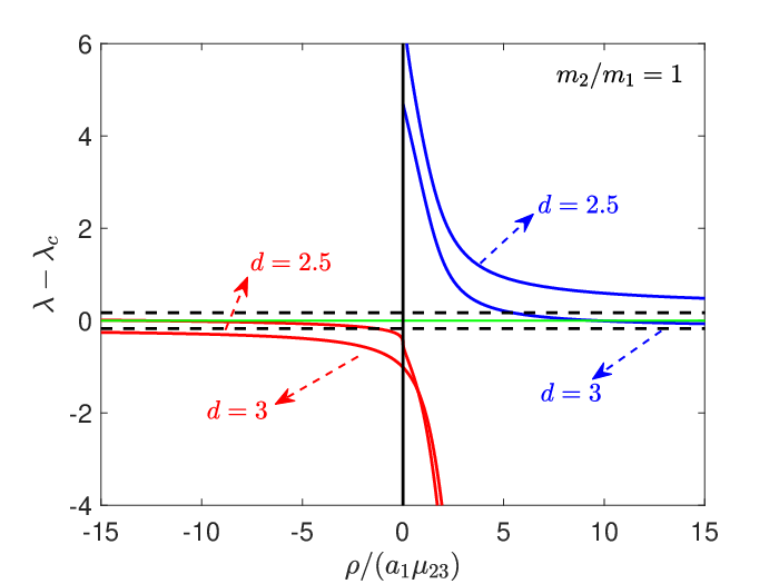
These figures are meant to establish the somewhat unusual presentation, where is the distance coordinate while we have assumed . The variation with is substantial but only appearing through the ratio to . The extreme limits of are shown in Fig. 3 as the straight horizontal dashed lines. The values for are the ultimate optimum for occurrence of the Efimov effect. Comparing to Fig. 2, we emphasize that these features are only valid for .
The left hand side of Fig. 3 is the lowest for negative . This function continues smoothly through on the right hand side where is positive. The divergence towards corresponds to the two-body bound state between the identical particles. It is irrelevant in connection with the Efimov state with completely different structure. Instead the possible Efimov states for must be supported by the second which for this zero-range interaction is diving down and approaching the same value (black dashed line, or infinite ) above as for large and . The qualitative behavior is the same for the two chosen examples of and equal masses as well as for other choices of variables. The quantitative differences shall be discussed further on in this report.
3.2 Basic properties
The Efimov effect is most easily understood for constant independent of distance. If this constant value is lower than the critical infinitely many states occur, whereas a value higher than does not support any bound state. Generalizing this schematic description we conclude that the Efimov effect with infinitely many bound three-body states occur if and only if is below in an infinitely large region of space. This is seen to be the case for both signs of in Fig. 3 as it should for for two infinitely large scattering lengths in three spatial dimensions. We emphasize that the -solutions for both positive and negative meet the Efimov condition (below the green line) for sufficiently large .
These conclusions and their dependencies on , , , and to be discussed later in this report. However, before proceeding with this we shall present a few other crucial properties. The wave functions, , arising from solving are, provided that and is constant in a sufficiently large region of , given by
| (15) |
where is the modified Bessel function of second kind. When the energy approaches zero this expression reduces to
| (16) |
where is a phase depending on the boundary condition at . The value of is either the small-distance range limit or the small where the potential crosses the threshold value corresponding to . The many bound states arise for different energies, , through the number of oscillations of the Bessel function for this energy. This form of the wave function implies scaling properties between neighboring states
| (17) |
Clearly infinitely many bound states correspond to infinitely many oscillations, that is for an infinitely large -space. In the present context the large -limit is given by the scattering length where the potential falls off exponentially, that is, it ceases to behave as . Thus we can rather accurately estimate the number of bound states in this available interval by counting the corresponding number, , of possible oscillations. We get
| (18) |
which diverge as . This discussion implies that the rigorously defined Efimov effect with infinitely many bound states only can occur for . However, even for finite there may be a finite number of bound states with precisely the same wave function properties. Thus, the number of such Efimov states is much more important than occurrence of the strict Efimov effect. The number of states is directly proportional to , which is a measure of the distance below the critical threshold for occurrence of the effect.
These derivations and considerations are strictly only valid for -independent , but rather accurate when the -variation is weak over intervals extended over more than a few oscillation of the wave function in Eq. (16). It is here important to appreciate the scale on the abscissa of Fig. 3, where is in units of the scattering length. The size of the variation of the curves over appropriate intervals are then easily visually deceiving, since the spatial extension of the states may be smaller than the scale of the variation. We maintain this -axis because it contains the full dependence on both and . In any case the qualitative features are correctly described.
So far the discussion has only rephrased known properties for three spatial dimensions (), total angular momentum zero (), and two infinite scattering lengths. After having defined the essential ingredients in the known cases, we shall extend to other and values as well as to arbitrary mass ratios, . We shall still concentrate on the -dependence while assuming the other two scattering lengths are equal and numerically very large.
4 Properties of Efimov states
The qualitative occurrence conditions can be elaborated to extract quantitative values of the theoretical variables. This means first of all relations between critical values for , , and , and second number of states and scaling properties. After the qualitative discussion we continue and present more quantitative results. We first connect to the more studied cases of , and afterwords we describe the dependence on smaller and non-integer values of . We shall present results with focus on the important but relatively unknown -dependence.
4.1 Occurrence of the Efimov effect
From Fig. 3 we confirm that the Efimov effect is always present for this case of two infinitely large scattering lengths in , independent of masses and size and sign of . The monotonous hypersherical angular eigenvalues at infinity both approach the same value below the critical number, . Then there is necessarily an infinite interval below and the Efimov effect exists in this case. However, this conclusion is crucially depending on , , and .
 |
 |
 |
 |
 |
 |
In Figs. 4 we show how the angular eigenvalues vary for different choices of these variables. For simplicity we have plotted all the relevant ’s as functions of , that is reflected in for negative . The overall picture is as in Fig. 3 with two curves both approaching the same asymptotic large-distance value from below and above, respectively. The decisive feature is whether this asymptotic value of is either below or above , which determines the existence or not of the Efimov effect.
The behavior of is monotonous not only as function of , but also as function of each of the variables, , , and . The asymptotic values for large are significant indicators. It moves upwards in Figs. 4 when increases, and when and decrease. This last fact indicates that large values of (two identical heavy particles and one light) are clearly more convenient for the appearance of the Efimov states than just the opposite (small values, corresponding to two light particles and one heavy).
The figures also reveal very flat (red) curves corresponding to the unbound case of . But also the blue curves for are very flat after a fast initial decrease from the starting points. Here it is important that the -axes are the hyperradius in units of the scattering length . The approximations of constant are therefore very appropriate.
In the limit of the Efimov effect is not present for any choice of variables. This possibility therefore disappears somewhere between and . The precise critical -value depends on both and . For given the curves are moved upwards with increasing and decreasing . Thus for sufficiently large , there are critical values of both and corresponding to crossing of .
The conclusion is that to rigorously have the Efimov effect the asymptotic -value must be below , and then the effect exists for both signs of . However, in practice these schematic curves must fall off much faster when becomes comparable to . The infinite series of bound Efimov states are then abruptly cut off. Still a finite number of bound states may be present and furthermore they may have properties (like universality and scaling) precisely (or approximately) as genuine Efimov states. This might happen at relatively small distances on the unbound branch even when the asymptotic is above . Thus, properties of a finite small number of states are even more interesting than strict occurrence of the effect.
4.2 Dependence for
Three dimensions are very well studied. We shall therefore only use this limit to set the stage while emphasizing the aspects of interest in the present context. The Efimov effect is present for two infinite -wave scattering lengths for all masses for . On the other hand, the effect only exists for non-zero -values when the mass ratio between the two heavy and the light particle exceeds critical values. We find for , respectively. The results for the higher -values are probably only of academic interest and are well known [1; 15].

The number of Efimov states is always finite in practice and very often also very small. The states are located below the limiting large scattering lengths but outside both the radius of the short-range potential and the critical crossing point, clearly seen on Fig. 3 in the side, where the blue curve takes negative values. The number of states is estimated analytically in Eq. (18), that is proportional to and the related logarithm. The crucial dependence is shown in Fig. 5 for both signs of and for different mass ratios.
The value of is the distance from to on figures similar to Fig. 3. The curves on the positive -side corresponding to a bound heavy-heavy subsystem increase dramatically before saturating at large at values increasing with mass ratio. The threshold values of zero correspond to -values of the crossing point where in Fig. 3. On the unbound (negative) -side we observe the opposite behavior of a slightly increasing with decreasing size of or equivalently increasing . This counter intuitive behavior is due to extension of the available space towards smaller distance, that is the earlier crossing of , see Figs. 3 and 4. The limit here is the short-range radius.
In all cases the size of is unpleasantly small even if multiplied by a sizable value of to produce the number of bound states in the accessible region of space. A realistic estimate could be , where is , resulting in only a few Efimov states for all . Closely related to the number of states is the scaling between the possible states, see Eq. (17). Unless is negative and very large, the scaling factor is very large for moderate mass ratios. Thus, the relative position of a few Efimov states would depend strongly on the precise value of , which in practice prevent universal prediction of these positions.
4.3 Dependence for
Decreasing from we know that the Efimov effect has disappeared all together in the limit, independent of any choice of variables. The questions are therefore where the disappearance takes place depending on mass ratio and angular momentum. We know from Figs. 4 that larger mass ratio increases the distance from the critical and consequently the -value increases. The same trend remains for all other , where the existence of the Efimov effect depends on the masses.

We show in Fig. 6 the corresponding critical mass as function of for different . Since the mathematics applies to any we also give results for . We notice the almost symmetric behavior around for . The minimum critical mass around allows the existence only in a region around . For higher values of , the minimum critical mass shifts to higher values of . The precise numbers for at are already given above but now we also see the variations as steep increases as decreases. The higher the more compensation is needed from increasing the mass ratio. Higher -values could also be calculated but we refrain.
The strict limit for is less favorable than the condition for large . This is obvious already for physical reasons since these limits (large ) and (small ) on the plots correspond to either three or two contributing subsystems, respectively. In Fig. 6 we present the critical masses as functions of for both and the ultimate limit of which can support more states. The difference between these estimates gives an interval for occurrence of Efimov states depending slightly on the third scattering length. The small bump on the curve is numerical inaccuracy in this extreme limit.
For equal masses and the difference is that the critical value of is pushed from () to (). For other given mass ratios we may read off the critical -value allowing Efimov states in both these extreme limits. When decreases towards the critical masses increase dramatically. A closer inspection of the governing equations in Eq. (13) reveals a corresponding unlimited increase, that is sufficiently large mass ratio allow Efimov states for any .
For the limits of large and small are almost indistinguishable. This may be understood from the fact that Efimov states are only allowed for -waves between at least two subsystems. This implies that finite angular momenta must be attached to the remaining subsystem in the present work labeled by . Then the corresponding -wave scattering length does not enter the Efimov equations.

As discussed for , we can also in the general cases calculate the expected number of states and the corresponding scaling from Eqs. (17) and (18). In Fig. 7, we show examples for different -parameters as functions of the variable. The appearance and explanations are the same as in Fig. 5 for both bound and unbound cases, threshold and saturation behavior. The numbers are larger because we have chosen a much larger mass ratio. Still the conclusions hold about only a few Efimov states and an unfortunate large scale parameter with huge variation close to the threshold at the bound side. However, this variation has essentially no physical impact since the interval is too small to support bound states.
5 Translation of
The dimension parameter, , is appealingly a measure of the spatial dimension varying between and . While this is rigorously correct in the two limits, it is unfortunately much more complicated for intermediate non-integer values. A proper physical interpretation, or a direct translation, is so far only available for two particles [16]. The problem can be formulated in ordinary three spatial dimensions where the effective dimension, , has to be related to confinement by an external potential. Then one coordinate is squeezed by such external walls varying from being at infinity to practically zero, which means much smaller than the short-range potential responsible for the properties.
It is physically obvious that the walls of the external potential have no effect on a system of much smaller spatial extension, and, vice versa, crucial for a system of larger natural extension. Thus the size of the system is decisive, as described in [16; 9], where a universal result is given for two particles held together by a spherical gaussian short-range potential and squeezed by a one dimensional external oscillator potential defined by a length parameter, .

The resulting relation for ( is the gaussian range) as function of is shown in Fig. 8 where the size of the system enters through the factor , where () is the scattering length of the two-body potential. This relation is parameterized as
| (19) |
where the constants take the values .
The qualitative behavior is seen to be that a large external field length, , is not noticed by the system, which therefore lives in just the ordinary three-dimensional space, i.e., . In the opposite limit, when the squeezing length approaches zero, the system is very much confined along the squeezing direction, corresponding therefore to . These two limits are connected by the curve in Fig. 8, which we emphasize is only strictly valid for two-particle systems. The generalization to three particles is not available at the moment, since an elaborate set of calculations are necessary for three particles in external fields implying complications as for a four-body problem. However, we anticipate qualitatively similar correspondence between and an external field. For now the two-body relation shown in Fig. 8 and Eq.(19) is sufficiently indicative for the investigations in the present report.
6 Conclusions
We use the hyperspherical expansion method with one uncoupled single adiabatic potential and the dimension parameter, , in the centrifugal barrier. We assume two identical bosons with two infinitely (equal) large -wave scattering lengths against the third particle, and , which allow existence of the Efimov effect in three dimensions. We then investigate dependence on the finite scattering length () between the two identical bosons, while varying the dimension parameter, the mass ratio, and total angular momentum. The Efimov effect, the scaling and number of Efimov states are large-distance phenomena and independent of short-range attraction. We consequently use the simple zero-range formulation.
We distinguish between occurrence of the Efimov effect and the finite number of practically accessible Efimov states. Both, the effect and all the corresponding states, disappear as the dimension is decreased towards two dimensions. When all masses are equal and the angular momentum is zero the effect disappears for and when the third scattering length is infinitely large and zero, respectively. We provide information about critical dimensions and critical masses for different angular momenta. We extract the scaling parameter and estimate the number of Efimov states as function of the third scattering length.
We discuss specifically the qualitative difference between results for different signs of corresponding to bound or unbound identical two-boson system. If the effect exists, the number of Efimov states is on the unbound side both proportional to the scaling parameter and limited to the number of possible wave function oscillations before reaching the large scattering length. On the bound side the number of states is given in the same way except for an additional restriction to be outside a radius varying weakly with . If the Efimov effect strictly does not exist, still a few Efimov states might be allowed on the unbound side while forbidden on the bound side.
Finally, we provide a qualitative relation between dimension parameter and a length parameter of an external field used to squeeze the spatial dimension of the system from to . The precise size of the external field in a three-body calculation is at present only estimated. However, a firm conclusion is that a reduction of the available space parameterized by unambiguously leads to disappearance of both, effect and all Efimov states. We provide at the moment only a qualitative estimate of the function translating the -parameter into precise size and shape of the external squeezing potential.
In summary, we have calculated occurrence conditions and properties of Efimov states depending on dimension, the third scattering length, masses, and angular momentum. All results are possible to test in practice in present day laboratories.
References
- [1] E. Nielsen, D. V. Fedorov, A. S. Jensen, and E. Garrido, Phys. Rep. 347, 373 (2001).
- [2] P. Naidon and S. Endo, Rep. Prog. Phys. 80, 056001 (2017).
- [3] M. Kunitski et al. Science 348, 551 (2015).
- [4] J. Johansen, B. J. DeSalvo, K. Patel and C. Chin, Nature Phys. 13, 731 (2017).
- [5] T. Kraemer et al., Nature 440, 315 (2006).
- [6] Q.-Y. Liang et al. Science 359, 783 (2018).
- [7] C. Chin, R. Grimm, P. S. Julienne, and E. Tiesinga, Rev. Mod. Phys. 82, 1225 (2010).
- [8] J. H. Sandoval, F. F. Bellotti, M. T. Yamashita, T. Frederico, D. V. Fedorov, A. S. Jensen, N. T. Zinner, J. Phys. B: At. Mol. Opt. Phys. 51 , 065004 (2018).
- [9] D.S. Rosa, T. Frederico, G. Krein, M.T. Yamashita, Phys.Rev. A 97 050701 (2018).
- [10] J. Levinsen, P. Massignan and M. M. Parish, Phys. Rev. X 4 , 031020 (2014).
- [11] M.T. Yamashita, F.F. Bellotti, T. Frederico, D.V. Fedorov, A.S. Jensen and N.T. Zinner, J. Phys. B 48, 025302 (2015).
- [12] A.S. Jensen and D.V. Fedorov, Europhys.Lett. 62, 336 (2003).
- [13] L. J. Wacker et al., Phys. Rev. Lett. 117, 163201 (2016).
- [14] V. Efimov, Yad. Fiz 12, 1080 (1970); Sov. J. Nucl. Phys. 12, 589 (1971).
- [15] O. I. Kartavtsev and A. V. Malykh, Phys. Rev. A 74, 042506 (2006).
- [16] E. Garrido, A.S. Jensen, R. Álvarez Rodríguez, to be published, (2018).