On local Dressians of matroids
Abstract.
We study the fan structure of Dressians and local Dressians for a given matroid . In particular we show that the fan structure on given by the three term Plücker relations coincides with the structure as a subfan of the secondary fan of the matroid polytope . As a corollary, we have that a matroid subdivision is determined by its 3-dimensional skeleton. We also prove that the Dressian of the sum of two matroids is isomorphic to the product of the Dressians of the matroids. Finally we focus on indecomposable matroids. We show that binary matroids are indecomposable, and we provide a non-binary indecomposable matroid as a counterexample for the converse.
1. Introduction
Let be an algebraically closed field of characteristic with a non-trivial, non-archimedean valuation. The tropical Grassmannian is a rational polyhedral fan parametrizing realizable -dimensional tropical linear spaces in the tropical projective space . These are contractible polyhedral complexes arising from the tropicalization of -dimensional linear spaces in the projective space . The tropical Grassmannian is the tropical variety obtained from the tropicalization of the Plücker ideal generated by the algebraic relations among the -minors of a -matrix of indeterminates. It is the tropicalization of the Grassmannian Gr. Its study has been initiated by Speyer and Sturmfels [26]. In the paper the authors focus in particular on the tropical Grassmannian , exhibiting a bijection with the space of phylogenetic trees with labeled leaves.
Herrmann, Jensen, Joswig and Sturmfels [11] studied the Dressian Dr, an outer approximation of the tropical Grassmannian which parametrizes all -dimensional tropical linear spaces in . This is the tropical prevariety defined by the three term Plücker relations among the generators of . These relations induce the Plücker fan structure on Dr. From work of Speyer [24] it follows that a point is in the Dressian if and only if it induces a matroid subdivision of the hypersimplex . This endows Dr with a secondary fan structure as subfan of the secondary fan of . In [11], the authors proved that for the two fan structures coincide.
The Grassmannian Gr can be stratified in strata consisting of points with coordinates equal to zero if and only if they are not indexed by a basis of a matroid. As remarked in [11], a similar stratification can be considered in the tropical setting. In particular, we can look at the intersection of the Dressian Dr with each of the open faces of . The intersection is not empty only if the face corresponds to a matroid of rank on . This motivates the authors to give a similar definition for the local Dressian Dr of a matroid . In the article, they focused exclusively on this construction for the Pappus matroid. In our paper, we provide more examples and we analyze more deeply the properties of local Dressians.
Local Dressians can also be endowed with two fan structures: one coming from the Plücker relations, one as a subfan of the secondary fan. Our main contribution is Theorem 14 which states that the two fan structures coincide. The proof is based on a careful analysis of the subdivision induced by a point in the local Dressian on the -dimensional skeleton of the matroid polytope. From our study it follows that a matroid subdivision is completely determined by its restriction to the -skeleton.
We then focus on local Dressians of disconnected matroids. We show that the local Dressian of the direct sum of two matroids is the product of their local Dressians. Again, the key step in the proof is to look at the -dimensional skeleton of the matroid polytope.
Finally, we move our attention to indecomposable matroids, i.e., matroids which do not admits matroid subdivisions of their matroid polytopes. The local Dressians of such matroids are linear spaces. We prove that binary matroids are indecomposable. Moreover, we give a counterexample for the converse, exhibiting a indecomposable non-binary matroid.
Many questions related to the indecomposability of matroids arose during the work for this manuscript. We conclude with a short section collecting them, including a conjecture.
Acknowledgments
We are very grateful to Takayuki Hibi and Akiyoshi Tsuchiya for the kind hospitality and the organization of the Summer Workshop on Lattice Polytopes 2018. Furthermore, we are indebted to Alex Fink for suggesting us to look at the matroid of Preposition 32. We also thank Michael Joswig and Felipe Rincón for their useful comments. Research by the first and second author is supported by the Einstein Foundation Berlin. Research by third author is carried out in the framework of Matheon (Project MI6 - Geometry of Equilibria for Shortest Path) supported by Einstein Foundation Berlin. The authors would also like to thank the Institute Mittag-Leffler for its hospitality during the program Tropical Geometry, Amoebas and Polytopes, where the collaboration started.
Notation
Before beginning, we fix some notation. Given non-negative integers, we define the sets , and . Moreover, given and , we use the notation . Furthermore, we denote the all ones vector by .
2. Tropical Grassmannians and tropical linear spaces
We begin with some basics about tropical geometry following Maclagan and Sturmfels [17], focusing in particular on the definition of tropical Grassmannian. We work over the tropical semiring , where arithmetic is defined by and .
Let be an algebraically closed field of carachteristic with a non-trivial non-archimedean valuation . Examples are the field of Puiseaux series and their generalizations with real exponents; see Markwig [18]. Given a polynomial ,
its tropicalization is
The tropical hypersurface trop is defined as the set of points such that the minimum in trop is attained at least twice. Given an ideal , the tropical variety trop is the intersection of the tropical hypersurfaces trop, with . A tropical prevariety is the intersection of finitely many tropical hypersurfaces. Any tropical variety is a tropical prevariety as it is the intersection of the hypersurfaces of a tropical basis; see Hept and Theobald [10] and [17, Section 2.6] for more details.
Any vector defines a partial term order on the polynomial ring . Given an homogeneous ideal the set of initial ideals endows with the structure of polyhedral complex called Gröbner complex. The following result, known as Fundamental Theorem of Tropical Algebraic Geometry, gives the connection between algebraic and tropical varieties, and subcomplexes of the Gröbner complex.
Theorem 1 ([17, Theorem 3.1.3]).
Let be an ideal in and its variety intersected with the torus . The following sets coincide in :
- (1)
the tropical variety trop;
- (2)
the closure in of set of vectors such that does not contain a monomial.
- (3)
the closure in of the set .
When working with homogeneous polynomials it makes sense to consider tropical hypersurfaces and varieties in the tropical torus or in its compactification . We will adopt both interpretations in this paper, making sure to specify which one we are considering.
Now, let be the polynomial ring in variables
We consider the Plücker ideal in generated by the algebraic relations among the -minors of any -matrix in any field. The Grassmannian is the variety . The ideal is generated by quadrics. The tropical Grassmannian is the tropical variety . It is a pure -dimensional rational polyhedral fan in .
The study of tropical Grassmannian was initiated by Speyer and Sturmfels [26]. The authors focused on and the special case . The fan structure and the homology of the tropical Grassmannian is studied in [11].
Theorem 2 ([26, Theorem 3.4 and Corollary 4.5]).
The tropical Grassmannian is characteristic-free and coincides with the space of phylogenetic trees with labeled leaves.
Classically, the Grassmannian Gr is an example of a moduli space. It parametrizes the -dimensional subspaces of a -dimensional -vector space. A -dimensional linear subspace of can be represented by a full rank matrix. The -minors form the Plücker vector which is a point on the Grassmannian. This surjective map from linear spaces to Plücker vectors is called the Stiefel map.
Now, let be a vector in the tropical Grassmanian . For each subset , consider the tropical linear polynomial
| (1) |
and define as the intersection of the tropical hyperplanes defined by , as varies over all elements in . Then, is the tropicalization of a classical -dimensional linear space.
Speyer in [24, Proposition 4.5.1] showed that every tropicalization of a linear space arises this way. Indeed, any classical linear space has Plücker coordinates. Taking the valuation of each Plücker coordinate yields a vector such that coincides with the tropicalization of the linear space. We take the above as definition of realizable tropical linear space. The tropical Grassmannian is the moduli space of realizable tropical linear spaces.
Theorem 3 ([26, Theorem 3.8]).
The bijection between the classical Grassmannian and the set of -planes in induces a unique bijection between the tropical Grassmannian and the set of realizable tropical -planes in -space.
Let be a tropical matrix. The tropical Stiefel map sends the matrix to the vector of its tropical minors . More precisely, for any we have
The tropical linear spaces which lie in the image of the tropical Stiefel map are called Stiefel tropical linear spaces. These linear spaces have been studied by Ricón [23], Herrmann et al.[13], and Fink and Rincón [7]. Notice that not all tropical linear spaces arise in this way, i.e., the tropical Stiefel map is not surjective.
3. Matroids and Dressians
In this section we introduce the main characters of this paper: matroids and Dressians. The former are classical objects in discrete mathematics. They are an abstraction of the concept of linear independence. Nakasawa and Whitney introduced them independently in the 1930s. There are many cryptomorphic ways to define a matroid. We will present just one definition and focus on their relation to polyhedral structures. We refer the interested reader to Oxley [21] and White [28]. A matroid is a pair where is a finite set and is a non-empty collection of subsets of satisfying the base exchange property: whenever and are in and and , there exists and element such that is also in . The sets in are called bases. Each basis has the same number of elements, called the rank of . Given a subset , the rank of is . A flat of is a subset of such that for every we have .
Example 4.
Given a matrix with entries in a field , the pair consisting of the set of columns of and the collection of the maximally independent subsets of is a matroid .
Example 5.
Given a (finite) graph, the pair consisting of the set of edges and the collection of the maximally spanning subsets of is a matroid.
One of the fundamental questions regarding matroid is about their representabilty. A matroid is representable over a field if it is isomorphic to a matroid for a matrix with entries in . A matroid representable over the finite field with two elements is called binary. A ternary matroid is one representable over the finite field with three elements. A matroid that can be obtained from a graph as described in Example 5 is called graphical matroid. Graphical matroids are regular, i.e., representable over any field. It is a recent result of Nelson [20] that almost no matroid is representable. The following example provides non-regular matroids.
Example 6.
Let and the collection of subsets of with elements. The matroid is the uniform matroid . The uniform matroid is not representable over a field with less than elements. In particular, the matroid is not binary.
Example 7.
The Fano matroid is an example of a binary matroid that is only representable over fields of characteristic two. It is represented by all seven non vanishing -vectors of length three over a field of characteristic .
The following operations on matroids are derived from taking minors of matrices. Let be a matroid and . The deletion of from , denoted , is the matroid . The contraction of from , denoted , is the matroid . Any matroid that is the result of successive deletions and contractions of is called a minor of . The dual of , denoted , is the matroid . It is straightforward to verify that , and that .
We are most interested in the polyhedral point of view of defining and studying matroids. We fix as ground set. Let be the canonical basis of . For a collection of subsets of , we define the polytope
where . The -th hypersimplex in is the polytope
A subset is a matroid of rank on elements if the edges of are parallel to the edges of , i.e., they are of the form for distinct. The elements in are the bases and is a matroid polytope. The fact that this construction gives a matroid is a result of Edmonds [5]. See also Gelfand, Goresky, MacPherson and Serganova [8].
In terms of the matroid polytope, we have that
Moreover, where is the affine involution that sends to for each coordinate . In particular, the polytopes and are isomorphic.
We now move to the definition of Dressians. We will particularly highlight their connection with matroids and matroid polytopes. Among the quadric generators of the Plüker ideal are the three term Plücker relations
| (2) |
where and pairwise distinct. The Dressian is the tropical prevariety in defined by the Plücker relations. This means that for a vector in the Dressian the minimum of
| (3) |
is achieved at least twice, where and pairwise distinct. The name Dressian was proposed by Herrmann et al. [11] in honor of Andreas Dress who discovered these relations by looking at valuated matroids. We call a point in the Dressian valuated matroid. The three term Plücker relations endow Dr with the Plücker fan structure. The Dressian can be also viewed as a subcomplex in the tropical projective space . We will do this in the next section, when we introduce local Dressians.
It follows directly from the definition that the Dressian contains the tropical Grassmannian for any characteristic . From the results in Maclagan–Sturmfels [17], it follows that = as fans and only as sets. The tropical Grassmannian depends on the characteristic of the field and for due to the representability properties of the Fano matroid. This implies that the Dressian disagrees with the tropical Grassmannian for and . This fact is even reflected in their dimensions. The dimension of is of order for fixed , while the dimension of grows linear in , see [15, Corollary 32].
As we said, the Dressian is the intersection of tropical hypersurfaces coming from the three term Plücker relations. Note that these relations do not generate the Plücker Ideal for , but they generate its image in the Laurent polynomials ring , see [11, Section 2]. The tropical variety defined by the ideal generated by the three term Plücker relations coincides with the tropical Grassmannian.
The following proposition provides an upper bound for the number of elements in a tropical basis for the tropical Grassmannian , i.e., the number of tropical hypersurfaces defining .
Proposition 8.
The tropical Grassmannian has a tropical basis of size:
Proof.
Note that this is a better estimation of the minimal size of a tropical basis than the one that can be derived from a general degree bound given in [16, Example 9].
Our final goal for this section is to explain the relation of the Dressian to a general concept in polyhedral geometry. Let be a polytope in with vertices and dimension . Any vector induces a regular subdivision of . We think as a height function which lifts the vertex to the height . By projecting the lower faces of the convex hull we get a subdivision of . Vectors inducing the same subdivision form a relatively open cone. The collection of all these cones is the secondary fan of the polytope . The lineality space is the largest linear space contained in each cone of the fan. The secondary fan has a -dimensional lineality space that contains . In particular we may consider its image in .
A subdivision of is a matroid subdivision if each of its cell is a matroid polytope. Speyer proved a description of the Dressian in terms of matroid subdivisions.
Theorem 9 (Proposition 2.2 in Speyer [24]).
A vector lies in the Dressian if and only if it induces a matroid subdivision of the hypersimplex .
This description sees the Dressian as a subfan of the secondary fan of the hypersimplex , and define the secondary fan structure on . Suppose that . For each of cardinality , and , the points
define the vertices of a octahedron , which is a -dimensional face of the hypersimplex . A point in the Dressian induces a matroid subdivision of . According to which of the three inequalities and equations in (3) are satisfied, the subdivision induced by on , determines one of the three possible subdivision of the octahedron in two quadrilateral pyramids or the trivial subdivision. Herrmann et al. [11] showed that for the Plücker fan structure coincides with the secondary fan structure. In the next section we will prove that this holds in general.
For any valuated matroid , we can define in the same way as we did for points in the Grassmanian in Section 2. We call such a tropical linear space. Note that, as there are valuated matroids that are not in the tropical Grassmanian, there are tropical linear spaces which are not realizable. If then all the faces of the subdivision induced by must be polytopes of matroids representable in characteristic ; see [25, Example 4.5.4] and [15, Proposition 34].
Given a valuated matroid , any point defines a matroid by taking the face from the regular subdivision of that is minimized in the direction of . In other words, the bases of are the sets such that is minimal. A loop in a matroid is an element which is contained in no bases. The notation of a linear space in (1) generalizes to an arbitary Plücker vector of its realizability. The following is a combinatorial description of such a tropical linear space.
Proposition 10 ([24, Proposition 2.3]).
The tropical linear space consists of exactly all points such that has no loops.
For each loopless matroid whose polytope appears in the regular subdivision induced by , there is a corresponding polyhedral cell in given by the closure of all the points such that . This way the tropical linear space has the structure of a polyhedral complex. A cell is bounded in this complex if and only if has no coloops. The subcomplex of bounded cells is the tight span. Note that the polyhedral structure of is not unique. We will illustrate this by looking at the recession fan of .
Whenever in the tropical projective space has only and as values, the tropical linear space coincides with the Bergman fan of the matroid whose bases are the coordinates where is . This is also the recession fan of . The Bergman fan has a natural fan structure by the above arguments. We can equip the Bergman fan with a finer structure in the following way: for each flat of , i.e., closed set, let be a ray in the Bergman fan. And for every flag of flats we get a cone generated by . When is any valuated matroid and , then is locally near the same as the Bergman fan of the matroid . For further details see [6], [1] and [17, Chapter 4]. Moreover, the introduction of Hampe [9] gives a broad overview about properties and developments of tropical linear spaces.
4. Local Dressians
Let be a matroid on the set of rank . Let be the number of bases of . We consider the variety in defined by the ideal obtained from the Plücker ideal by setting all the variables to zero, where is not a basis of . The variety is the realization space of the matroid . It parametrizes all the -dimensional linear subspaces of whose non-zero Plücker coordinates are the bases of . In particular if and only if the matroid is not representable over . This gives a stratification of the Grassmannian Gr, where the strata are defined as
A variation of Mnëv’s Universality theorem implies that the strata can be complicated as any algebraic variety.
Remark 11.
For the reader familiar with toric geometric, consider the Grassmannian Gr over the complex numbers . The algebraic torus acts on by . The action is linear so it maps subspaces to subspaces. Therefore, it induces an action on the Grassmannian Gr. Given a point , the closure of the orbit is a toric variety. Let be a point in the stratum defined by . The image of through the moment map is the matroid polytope . For further reading we refer to [8].
We now look at a similar local construction for the Dressian, i.e., we look at the Dressian of a matroid . This construction has been introduced by Herrmann et al. [11]. In the article the authors focus just on a single example where is the Pappus matroid of rank three on nine elements.
The Dressian of a matroid is the tropical prevariety in given by the set of quadrics obtained from the three term Plücker relations by setting the variables to zero, where is not a basis of . The Dressian contains the Dressians of all matroids of rank on elements as subcomplexes at infinity.
Let us be more precise. From the coordinatewise logarithmic map we get a homoemorphism . The tropical projective space is a compactification of the tropical torus , such that the pair is homeomorphic to .
Given a non-empty subset of , we define the set
The image of the sets through the quotient map give a stratification of the boundary of . See Section 5 of Joswig [14] for further details.
The intersection of the closure of the Dressian in the tropical projective space and the boundary stratum agrees with the local Dressian . Therefore the Dressian contains the Dressians of the matroid as subcomplex at infinity.
Remark 12.
Our definition of the local Dressian of the uniform matroid agrees with the definition of the Dressian and is bases only on the three term Plücker relations. The definition of the local Dressian given in [11, Section 6] and [17, Definition 4.4.1] takes all quadratic Plücker relations into account. These definitions agree, see [2, Example 2.32]. In the paper, the authors call the elements in our definition of the Dressian weak matroids and the elements coming from all quadratic Plücker relations strong matroids over the tropical hyperfield.
The following statement follows from the definition of Dr and Theorem 9.
Corollary 13.
A vector lies in the Dressian if and only if it induces a matroid subdivision of the matroid polytope .
Therefore we have again two fan structures on the Dressian of a matroid : one induced by the Plücker relations and one induced by the secondary fan.
Theorem 14.
Let be a matroid of rank on elements. The Plücker fan structure coincides with the secondary fan structure on .
Proof.
First, we take vectors and lying in the same cone of the secondary fan. They induce the same subdivision of the matroid polytope , in particular of the -dimensional skeleton. Therefore and satisfy the same three term Plücker relations and lie in the same cone of the local Dressian equipped with the Plücker structure.
Now we focus on the viceversa. We take and lying in the same Plücker cone . This means that they satisfy the same equations and inequalities coming from the three term Plücker relations. By Corollary 13, they induce two matroid subdivisions and of . We want to show that . This will imply that are in the same secondary cone. By the fact that they satisfy the same Plücker relations, we know that as the -faces are either tetrahedra or octahedra. We pick a maximal dimensional cell in . We suppose that is not in . It means without loss of generality there are vertices and in the cell such that and do not lie in a maximal dimensional cell of . Let be a path in the vertex-edge graph of the cell . We pick a cell in that contains for some and there is no cell in containing .
Now we have that and are at most of distance two. So we can use the base exchange axiom in the definition of a matroid to construct up to six points giving the unique face of spanned by and . The following situations may arise.
- •
Either is a octahedron, then is subdivided in as , are in and is not. This is a contradiction to the fact that the subdivisions agree on the -skeleton.
- •
If is a pyramid, it cannot be subdivided, therefore is a face of and hence is a vertex of , and that contradicts our assumption.
- •
Similarly if is -dimensional, i.e., a square or a triangle.
Hence we conclude that both points and are in and hence the subdivisions and agree. ∎
Corollary 15.
The Plücker fan structure on the Dressian as a fan in coincides with the secondary fan structure.
Proof.
It is enough to consider the uniform matroid in the previous statement. ∎
Corollary 16.
Let , and and be two matroid subdivisions of the hypersimplex . If they induce the same subdivision on the -skeleton, or equivalently on the octahedral faces of , then and coincide.
Remark 17.
The above statement extends Proposition 4.3 and Theorem 4.4 by Herrmann et al. [11] and is the key in the algorithm in Section 6 of Herrmann et al. [13] for computing (local) Dressians. Note that the abstract tree arrangements in Section 4 of Herrmann et al. [11] are a cover of the -skeleton of the hypersimplex for and the metric condition guarantees that the height functions agree on all three maps that contain a given vertex.
A connected component of is a minimal non empty subset with the property that is the same for every base of . Connected components of partition . If is the only connected component, we say that is connected. We derive the following characterization of the lineality space which follows from the characterization of the dimension of a matroid polytope in terms of connected components by Edmonds [5] or Feichtner and Sturmfels [6]. Together with the fact that the secondary fan of a set of vertices has a lineality space of the same dimension as the affine dimension of the set of vertices.
Corollary 18.
Let be the number of bases of a matroid on elements and with connected components. The lineality space of the Dressian in is of dimension .
Proof.
Adding a linear functions to the height function of a regular subdivision does not change the subdivision. Therefore the linealty space is the image of the map with . ∎
Example 19.
The local Dressian of the uniform matroid coinsides with the Dressian . This is a -dimensional pure balanced fan in consisting of three maximal cells and a -dimensional lineality space.
Example 20.
The local Dressian of the matroid is a -dimensional linear space in spanned by and . The corresponding matroid polytope is a square, which has no finer matroidal subdivision.
Let us discuss two examples of local Dressians of non-regular connected ternary -matroids. These are matroids that are representable over the field with three elements, but are not representable over the field with two elements.
Example 21.
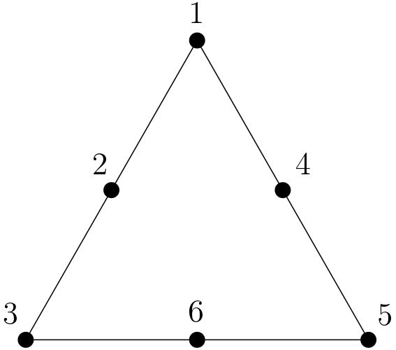
Let be the matroid on 6 elements and rank 3 whose bases are , see Figure 1. The polytope is full dimensional so the local Dressian has a lineality space of dimension in . The local Dressian is -dimensional and consists of three maximal cones. These cones correspond to the vertex split with the hyperplane and two -splits, i.e., a subdivision into three maximal cells that intersect in a common cell of codimension . The three maximal cells of one of those -splits is illustrated in Figure 2.

Example 22.
Let be the connected matroid given by the bases:
The local Dressian consists of three maximal cones of dimension and a -dimensional lineality space in . In other words the polytope has four matroidal subdivisions. The trivial subdivision and three splits with respect to the hyperplanes , or .
Remark 23.
For any point in the local Dressian we can construct a tropical linear space , by taking the intersection over of the tropical hyperplanes defined by
Further details on tropical linear spaces can be found in [17, Section 4.4].
Proposition 24.
Let and be matroids such that is combinatorially isomorphic to . Then,
Proof.
A matroid subdivision of the polytope does not impose new edges. The isomorphism between the polytopes and induces a subdivision of as images of cells. Moreover, this subdivision is matroidal as the -cells are edges of . This subdivision is regular, as the map between and is a concatenation of a coordinate permutation, an embedding and a reflection. This follows from the explicit description in Remark 25. ∎
Remark 25.
It can be shown that the two matroid polytopes of and are combinatorially isomorphic if and only if the matroids are isomorphic up to loops, coloops or dual connected components. This is part of the work by Pineda-Villavicencio and Schröter [22].
The following statement deals with Dressians of disconnected matroids. Let and be matroids and with and disjoint. We define the direct sum of and as
Theorem 26.
Let and be matroids with disjoint element sets. Then
Proof.
We have the map
where for any and . To check that satisfies the tropical Plücker relations notice the following: any octahedron contained in must be of the form , with and octahedron contained in , or , with and octahedron contained in . Then the Plücker relations follow from those of and . In particular, the cone where lies is determined by the cones where and lie, so maps cones into cones.
To construct the inverse of , we fix a basis and we define the map
where and for any and any . It is straight forward to verify that the Plücker relations satisfied by imply that the projections and satisfy them as well. In particular, maps cones to cones.
Now we prove that is independent of the choice of basis . We do this by contradiction. Suppose it is not, without loss of generality we can assume there exist and , with and of distance 1 such that does not agree for these two choices. Clearly is the same for both choices, so we look at . Let be bases at distance 1. We have that the points form a square face of . This square can not be subdivided, so
But this means that the difference of for and is independent of the choice of . By connectivity of the graph of , we can conclude that is independent of the choice of .
We are left with proving that is the inverse of . First we check that for any we have that . To see this, notice that for any . But is a constant independent of , so in the tropical torus. Analogously, we get that .
Now we check the other direction, that is, for any we have . Consider two bases of at distance 1. Without loss of generality let them be and . We have that
We have already shown that is independent of the choice of , so we may assume . Hence, the above equals . By connectivity of the graph of , we get as we wanted.
Therefore, the maps and are bijective linear maps which send cones to cones, which implies . ∎
Remark 27.
The statement above generalizes Theorem 4 by Chatelain and Ramírez [4] which deals with sequences of weakly compatible hyperplane splits. While the article by Joswig and Schröter [15] provides the case of sequences of strongly compatible hyperplane splits and the matroid polytopes that occur in these matroid subdivisions. We refer to Herrmann and Joswig [12] for the definitions.
Let be a matroid . Two elements and in are parallel if . We denote this by . Remark that this implies that .
Theorem 28.
Let be a matroid and in . Then
and .
Proof.
Clearly, contains the circuit . Hence, the number of connected components of is the same as the number of connected components of . It follows that .
The projection that forgets the coordinates that correspond to bases that contain is surjective. Our goal is to show that this projection is injective if we quoten by the lineality spaces. Let and be a basis of that contains and . We may assume that as the lineality space of contains . Let be a basis of and of distance . That is , , , , form a square in the vertex-edge graph of . The set is a non-basis of distance to those four bases. Therefore, the square is not subdivided by the regular subdivision induced by . We conclude that and by our assumption . Iterating our argument shows that for any basis that contains . As the basis exchange graph of a matroid is connected. Therefore, we derive that the projection is injective up to lineality and therefore the desired isomorphism. ∎
5. Indecomposable Matroids
In this section, we begin with focusing on local Dressians of binary matroids, i.e., those matroids which are representable over the field with two elements. Recall that any matroid obtained from successive deletions and contractions form a matroid is a minor of . The following is a useful characterization of binary matroids in terms of their minors.
Proposition 29 (Tutte[27]).
A matroid is binary if and only if it has no minor isomorphic to the uniform matroid .
From Proposition 29 we derive a generalization of Theorem 3 by Chatelain and Ramírez [3] which states that a matroid polytope of a binary matroid can not be splited into two matroid polytopes.
Definition 30.
A matroid is said to be indecomposable if and only if its polytope does not allow a non-trivial matroid subdivision.
Corollary 31.
Let be a binary matroid. Then the local Dressian linear space. In particular, the matroid polytope is indecomposable.
Proof.
Let be a binary matroid and its matroid polytope. The -skeleton of the polytope does not contain a octahedral face as such a face corresponds to a minor isomorphic to the uniform matroid . From Corollary 16 we deduce that only has a trivial matroid subdivision. That is the Dressian is a linear space and is indecomposable. ∎
A matroid can be indecomposable even if its matroid polytope contains octahedral faces. Consider the simple matroid on elements and rank given by the ternary projective plane. This matroid is not binary and its matroid polytope has octahedral faces.
Proposition 32.
The local Dressian is a -dimensional linear space. In particular, the matroid is indecomposable.
Proof.
We will show the indecomposability by contradiction. We assume that is a proper connected submatroid of . Being a submatroid means that every basis of is a basis of . In this proof we will use the closure operators of the matroids and . Recall that the closure of a set is the maximal set that contains with . Here with maximal we mean that for every element we have . We denote by the closure of in and by the closure of in . They satisfy whenever .
The proof consists of five steps:
- •
There are two parallel elements in .
- •
Two lines in collapse to a line in .
- •
A quadrilateral in collapses to a point in .
- •
Three concurrent lines in collapse into a line in .
- •
Contradiction.
After each step, for improving the exposition, we reset the labeling. We make sure to clarify the new assigned labels. We do this in order to assure that there is no loss of generality. Keep in mind that for to be connected there is no line such that its complement is a single point. In particular there must be a least four points, i.e., four parallelism classes.
Our first step is to show that contains a pair of parallel elements. Suppose that the set is a basis of but it is dependent in . Either contains a parallel pair or is of rank as is loop free. In the latter case, let be not in the rank flat . This implies that the intersection of the lines is of rank in . As is not parallel to in then and, as is independent in , there is an element in . This means that and hence it is parallel to in .
Suppose now that and are two parallel elements in . Notice that there are at lest three elements not in . Moreover, has four elements, at least two of which are in . Then there exists an element such that is not in . Therefore, and are two different lines in which are contained in .
Suppose that the seven points on the two lines and in span a line in . There must be at least two points and outside this line in the connected matroid . Each of the three lines , and intersects the line in a different point in the projective geometry . This induces a bijection between and where elements are mapped to parallel elements in . Similarly, a bijection can be constructed by considering the lines from . These bijections do not agree and hence, there are at least four parallel elements in that span a quadrilateral in .
Suppose that is a quadrilateral in which collapses to a point in . Let , and , and . As is connected, there are at least three elements outside . Suppose that these points are exactly , and . Then forcing , and to be colinear in , and disconnected. So there is another point outside . In particular, three of the lines in passing through also pass through at least one point in the quadrilateral . Therefore they collapse in a single line in .
Suppose three concurrent lines passing through in collapse to a single line in . Let be the set of elements different from forming these three lines. As is connected there must be at least two elements outside . For each point, the lines passing through it and not induces a partition of in three subsets of size three, such that the elements in each subsets belong to the same parallelism class. The two partitions are transversal, therefore is in the same parallelism class. As the complement of is a line in , then is disconnected and we obtain a contradiction. ∎
Remark 33.
We actually proved a stronger statement, namely that the matroid does not contain a proper connected submatroid.
We end this section by showing that a finest matroid subdivision of contains only indecomposable matroids.
Proposition 34.
The cells of a finest matroid subdivision of correspond to binary matroids. In particular, they are indecomposable.
Proof.
Every matroid subdivisions of the hypersimplex is regular, as it is a sequence of compatible splits, i.e., subdivisions that divide into two maximal cells. See [15] and [12] for further details. Every regular matroid subdivision of is representable in characteristic as . Moreover, it is a finest subdivision if and only if it has maximal cells. The Main Theorem in [25] states that all cells in a subdivision of the hypersimplex are graphical and therefore binary whenever the subdivision is induced by a Plücker vector in and has maximal cells. This applies to the finest subdivisions of and hence the maximal cells are matroid polytopes of binary matroids and indecomposable. ∎
6. Open Questions
Several questions arise from the last section. We end this article by stating them and in particular, by making a conjecture.
A class of possible indecomposable matroids comes directly from the previous section. We conjecture the following generalization of Proposition 32:
Conjecture 35.
All matroids that arise from projective spaces over finite fields are indecomposable.
Notice that a direct consequence would be examples of indecomposable matroids which are only representable over a particular characteristic. While the direct sum of the ternary projective plane and the binary projective plane, i.e., fano matroid, is an indecomposable matroid which is not representable over any field. We also want to remark that as the ternary projective plane has a decomposable minor , a classification of indecomposable matroids can not relay on excluded minors.
Moreover, it would be interesting to find an efficient criterion to check indecomposability. In Proposition 32 we used that there does not exist a connected submatroid. We wonder whether a submatroid is in general a certificate of decomposability.
Question 1.
Does there exist two connected matroids and such that is strictly contained in but no matroid subdivision of has as a cell?
Notice that when is a uniform matroid then the corank subdivision has as a cell. But the corank function of does not necessarily satisfy local Plücker relations.
Example 36.
Let be a matroid with bases , , , and and be the matroid with the two bases and . Then the local corank lifting is and this vector is not in the local Dressian as it subdivides the square pyramid into two tetrahedra.
Our last question is about finest matroid subdivisions of hypersimplicies and is derived from Proposition 34.
Question 2.
Are all cells in a finest matroid subdivision of a hypersimplex matroid polytopes of indecomposable matroids?
References
- [1] Federico Ardila and Caroline J. Klivans. The Bergman complex of a matroid and phylogenetic trees. J. Combin. Theory Ser. B, 96(1):38–49, 2006.
- [2] Matthew Baker and Nathan Bowler Matroids over partial hyperstructures preprint arXiv.org/pdf/1709.09707, 2017.
- [3] Vanessa Chatelain and Jorge L. Ramírez Alfonsín. Matroid base polytope decomposition. Adv. in Appl. Math., 47(1):158–172, 2011.
- [4] Vanessa Chatelain and Jorge L. Ramírez Alfonsín. Matroid base polytope decomposition II: Sequences of hyperplane splits. Adv. in Appl. Math., 54:121–136, 2014.
- [5] Jack Edmonds. Submodular functions, matroids, and certain polyhedra. In Combinatorial Structures and their Applications (Proc. Calgary Internat. Conf., Calgary, Alta., 1969), 69–87. Gordon and Breach, New York, 1970.
- [6] Eva Maria Feichtner and Bernd Sturmfels. Matroid polytopes, nested sets and Bergman fans. Port. Math. (N.S.), 62(4):437–468, 2005.
- [7] Alex Fink and Felipe Rincón. Stiefel tropical linear spaces. J. Combin. Theory Ser. A, 135:291–331, 2015.
- [8] I. M. Gelfand, R. M. Goresky, R. D. MacPherson, and V. V. Serganova. Combinatorial geometries, convex polyhedra, and Schubert cells. Adv. in Math., 63(3):301–316, 1987.
- [9] Simon Hampe. Tropical linear spaces and tropical convexity. Electron. J. Combin., 22(4):Paper 4.43, 20, 2015.
- [10] Kerstin Hept and Thorsten Theobald. Tropical bases by regular projections. Proc. Amer. Math. Soc., 137(7):2233–2241, 2009.
- [11] Sven Herrmann, Anders N. Jensen, Michael Joswig, and Bernd Sturmfels. How to draw tropical planes. Electron. J. Combin., 16(2, Special volume in honor of Anders Björner): Research Paper 6, 26, 2009.
- [12] Sven Herrmann and Michael Joswig. Splitting polytopes. Münster J. Math., 1:109–141, 2008.
- [13] Sven Herrmann, Michael Joswig, and David E Speyer. Dressians, tropical Grassmannians and their rays. Forum Mathematicum, pages 389–411, 2012.
- [14] Michael Joswig. Essentials of tropical combinatorics. Book in preperation.
- [15] Michael Joswig and Benjamin Schröter. Matroids from hypersimplex splits. J. Combin. Theory Ser. A, 151:254–284, 2017.
- [16] Michael Joswig and Benjamin Schröter. The degree of a tropical basis. Proc. Amer. Math. Soc., 146(3):961–970, 2018.
- [17] Diane Maclagan and Bernd Sturmfels. Introduction to Tropical Geometry, volume 161 of Graduate Studies in Mathematics. American Mathematical Society, Providence, RI, 2015.
- [18] Thomas Markwig. A field of generalised Puiseux series for tropical geometry. Rend. Semin. Mat. Univ. Politec. Torino, 68(1):79–92, 2010.
- [19] Ezra Miller and Bernd Sturmfels. Combinatorial commutative algebra, volume 227 of Graduate Texts in Mathematics. Springer-Verlag, New York, 2005.
- [20] Peter Nelson. Almost all matroids are nonrepresentable. Bull. Lond. Math. Soc., 50(2):245–248, 2018.
- [21] James Oxley. Matroid theory, volume 21 of Oxford Graduate Texts in Mathematics. Oxford University Press, Oxford, second edition, 2011.
- [22] Guillermo Pineda-Villavicencio and Benjamin Schröter. Reconstruction of matroid polytopes. In preperation.
- [23] Felipe Rincón. Local tropical linear spaces Discrete Comput. Geom., 50:700–713, 2013.
- [24] David E. Speyer. Tropical linear spaces. SIAM J. Discrete Math., 22(4):1527–1558, 2008.
- [25] David E. Speyer. A matroid invariant via the K-theory of the Grassmannian. Adv. Math., 221(3):882–913, 2009.
- [26] David Speyer and Bernd Sturmfels. The tropical Grassmannian. Adv. Geom., 4(3):389–411, 2004.
- [27] W. T. Tutte. A homotopy theorem for matroids. I, II. Trans. Amer. Math. Soc., 88:144–174, 1958.
- [28] Neil White, editor. Theory of matroids, volume 26 of Encyclopedia of Mathematics and its Applications. Cambridge University Press, Cambridge, 1986.