Semi-Parametric estimation of plane similarities Application to fast computation of aeronautic loads

In our framework, we have at hand $K+1$ curves. $\tilde{C}$ is the reference curve and we assume that the $K$ other curves $C_{j},\ j=1,...,K$ are the images of $\tilde{C}$ by the transformation model described bellow. The $K$ curves are observed on the same random grid $\mathcal{D}_{N}:=\{X_{1},...,X_{N}\}$ where $(X_{i})_{i=1,...,N}$ are iid random variables with uniform distribution. Hence we have at our disposal

We will consider the following two cases

• i) $\tilde{C}$ is known everywhere: $\tilde{C}=(x,\tilde{f}(x))$, $\forall x\in[0,1]$,
  

• ii) $\tilde{C}$ is only known on $\mathcal{D}_{N}$: $\tilde{C}=(x,\tilde{f}(x))$, $\forall x\in\mathcal{D}_{N}$.
  

Before defining the transformation model linking the $K$ observed curves to the pattern $\tilde{C}$, one must ensure that the functions $f_{j}$, $j=1,...,K$ and $\tilde{f}$ are ”admissible”. This is the aim of the next definition:

Let now define the parametric family of transformation that we will put in action.

In the following, we define our transformation model.

Set $0<\theta_{0}<\theta_{1}<\frac{\pi}{2}$, and $0<\lambda_{min}<\lambda_{max}$. For any $\alpha:=(\theta,\lambda)\in\Theta=[-\theta_{0},\theta_{1}]\times[\lambda_{min},\lambda_{max}]$, set

$T_{\alpha}:=H_{\lambda}\circ S_{\theta}\circ R_{\theta}$

the composition of a rotation $R_{\theta}$, a rescaling $S_{\theta}$ applied on the $x$-axis, and a homothetic transformation $H_{\lambda}$ on the $y$-axis. More precisely

• $\bullet$

  $R_{\theta}$ is the rotation centered in $\begin{pmatrix}1\\ 0\end{pmatrix}$ and of angle $\theta$. That is
  

  	$\displaystyle R_{\theta}:[0,1]\times\mathbb{R}^{+}$	$\displaystyle\to[-A_{min},1]\times\mathbb{R}$
  	$\displaystyle\begin{pmatrix}x\\ y\end{pmatrix}$	$\displaystyle\to\begin{pmatrix}(x-1)\cos{\theta}-y\sin{\theta}+1\\ (x-1)\sin{\theta}+y\cos{\theta}\end{pmatrix},$

  with $A_{min}=\sqrt{1+y(0)^{2}}-1$.
  

• $\bullet$

  After rotating a curve, depending of the angle $\theta$, the resulting design space of the curve is generally no more [0,1]. Hence, we define the following transformation to re-position the curve on [0,1]:
  

  	$\displaystyle S_{\theta}:[-A_{min},1]\times\mathbb{R}$	$\displaystyle\to[0,1]\times\mathbb{R}$
  	$\displaystyle\begin{pmatrix}x\\ y\end{pmatrix}$	$\displaystyle\to\begin{pmatrix}\frac{x-a}{1-a}\\ y\end{pmatrix},$

  with $a$ is the real minimum value of the design space after rotating the curve.
  

• $\bullet$

  The scaling transformation of parameter $\lambda>0$ acting on the second coordinate of the curve:

  	$\displaystyle H_{\theta}:[0,1]\times\mathbb{R^{+}}$	$\displaystyle\to[0,1]\times\mathbb{R}^{+}$
  	$\displaystyle\begin{pmatrix}x\\ y\end{pmatrix}$	$\displaystyle\to\begin{pmatrix}x\\ \lambda y\end{pmatrix}.$

We now introduced the assumption that will be used:

• (A1): The functions $(f_{j})_{j=1,...,K}$, and $\tilde{f}$ belong to $\mathcal{F}_{\theta_{0}}$.
  

• (A2): For any $\theta\in[-\theta_{0},\theta_{1}]$, for any $x\in[0,1]$ and any $f\in\mathcal{F}_{\theta_{0}}$, the second coordinate of $R_{\theta}$ is positive.
  

• (A3): $\Theta=[-\theta_{0},\theta_{1}]\times[\lambda_{min},\lambda_{max}]$.
  

• (A4): $\tilde{C}$ is known on $[0,1]$.
  

• (A5): $\tilde{C}$ is known on the grid $\mathcal{D}_{N}$.
  

Thus, the transformation model considered is as follows:

Recall that we wish to adjust the reference curve $\tilde{C}$ on the other curves $C_{j}$ ($j=1,...,K$) by transformations defined in the previous subsection. Notice that these transformations act on both axis. For any $\alpha$, we want to compare the value of the transformed curve $(T_{\alpha}\tilde{C})(X_{i})$ with $f_{j}(X_{i})$. Since the abscissa points are affected by the transformation, we denote by $X_{i}(\alpha)$ the point such that $T_{\alpha}^{1}(X_{i}(\alpha))=X_{i}$. For that reason, we introduce the following definition:

To ease the notation, we finally set $x(\alpha):=x(\alpha,g)$, so $X_{i}(\alpha)=X_{i}(\alpha,\tilde{f})$. We consider the parametric regression model:

Where:

• $\bullet$

  $(X_{i})$ are iid with distribution $\mathbb{P}_{X}$. It is the design on which we observe the curves $C_{j}$;

• $\bullet$

  $\alpha_{j}^{*}=(\theta_{j}^{*}$,$\lambda_{j}^{*})$ is the couple of true parameters for each curve ($j=1,...,K$);

• $\bullet$

  $\epsilon_{j,i},\ \forall i=1,...,N,\ \forall j=1,...,K$ are iid $\mathcal{N}(0,\sigma^{2})$ random variables. These variables are assumed to be independent of $X_{i}$.
  

We consider the following model:

with $g(x)=2(\cos{\pi x}+1)$. We observe $f_{\lambda_{j},\theta_{j}}(x_{i})$ for $i=1,...,100$, for $J=25$ values of $(\lambda,\theta)$ with some iid errors $\epsilon_{ij}$.

• $\bullet$

  The observations points $x_{i},\ i=1,...,100$ are iid random variables with uniform distribution on $[0,1]$.

• $\bullet$

  The parameters are chosen randomly with the following arbitrary distribution $(\lambda,\theta)\hookrightarrow\mathcal{U}([0,15])\times\mathcal{U}([-\frac{\pi}{3},\frac{\pi}{30}])$.

• $\bullet$

  The errors are assumed to be $\mathcal{N}(0,0.01)$.

Results are given in Figure 1. The simulated data are shown in Figure 1 (a). Each of these curves is rescaled to $[0,1]$ to avoid numerical issues. The curve in blue is the reference curve. After the estimation of the parameters $\lambda_{j}$ and $\theta_{j}$, all curves can be rescaled back to their original space as shown in Figure 1 (b).

Rescaling the curves allows to easily choose the initial point of parameters for the optimization algorithm taking 1 for $\lambda$ and 0 for $\theta$.

An airframe structure is a complex system and its design is a complex task involving today many simulation activities generating massive amounts of data. This is, for example, the process of loads and stress computations of an aircraft. That is the computations of the forces and the mechanical strains suffered by the structure. The overall process exposed in Figure 2 is run to identify load cases (i.e aircraft mission and configurations: maneuvers, speed, loading, stiffness…), that are critical in terms of stress endured by the structure and, of course, the parameters which make them critical. The final aim is to size and design the structure (and potentially to reduce loads in order to reduce the weight of the structure). Typically for an overall aircraft structure, millions of load cases can be generated and for each of these load cases millions of structural responses (i.e how structural elements react under such conditions) have to be computed. As a consequence, computational times can be significant.

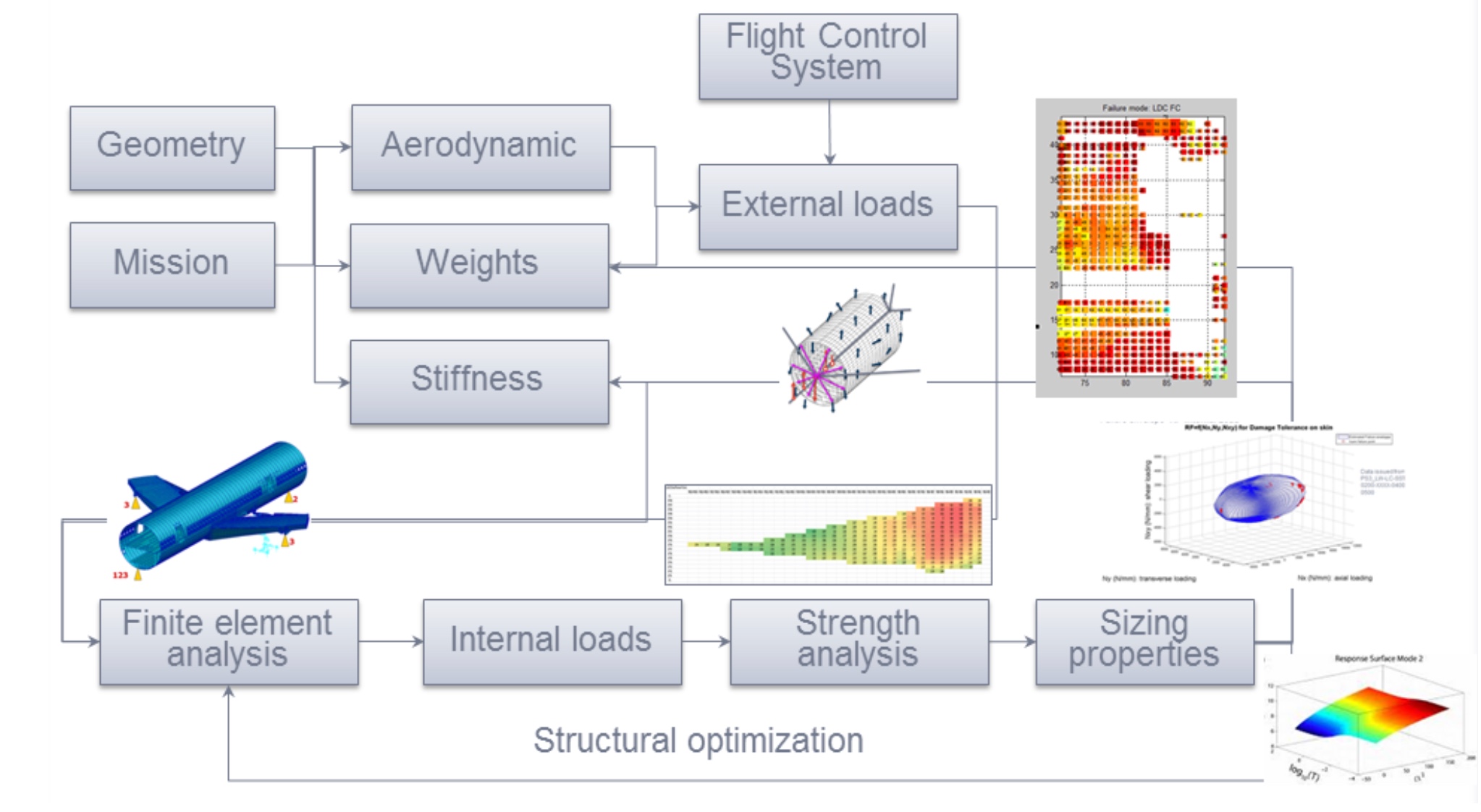
In an effort to continuously improve methods, tools and ways-of-working, Airbus has invested a lot in digital transformation and the development of infrastructures allowing to treat data (newly or already produced). The main industrial challenge for Airbus is to reduce lead time in the computation and preliminary sizing of an airframe as well as extracting value from already calculated loads. In this paper, we focus on the external loads of a wing: for each load case are calculated the shear forces (transverse forces near to vertical arising from aerodynamic pressure and inertia) and bending moments (resulting from the shear forces, they represent the flexion of the wing) such as shown in Figure 3.

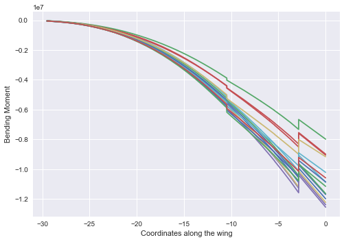
These external loads appeared to be extremely regular and one can legitimately suppose that it exists a link between all those curves. Indeed, it is natural to assume that it exists a reference bending moment (a reference curve) which can be morphed through a deformation model to give all the other curves.

In [6], the authors present an aeronautic model that computes the loads (forces and moments) on the wing of some aircraft model denoted by $ACM1$. They present several statistical methods in order to study these data. In this section, we will compare the method used in [6] with the model presented in Section 2 for a new aircraft model called $ACM2$. The data at our disposal represents bending moments of a wing (representing its flexion) of an aircraft calculated for 1152 different configurations (load cases). Each configuration is defined by 28 features (speed of the aircraft, mass, altitude, quantity of fuel, etc.), leading to a bending moment calculated on 45 stations along the wing. In a more formal way, we observe the couple $(X_{j},Y_{j})_{j=1,...,1152}$, where $X_{j}=(X_{j}^{1},...,X_{j}^{28})$ are the features and $Y_{j}=(Y_{j}^{1},...,Y_{j}^{45})$ is the bending moment. The idea is to predict the bending moment for different configurations. The data are represented in Figure 4.

Due to the discontinuities at the $3^{rd}$ and $20^{th}$ stations, we apply our methodology to each section independently. Then, each section can be represented by its minimum and maximum values, and by its rotation and scaling coefficients $\lambda_{j}$ and $\theta_{j}$. Figure 5 assess the quality of the matching process (the reference curve used is the average bending moment).

Thus the dimensional space of the outputs is reduce to 12 instead of 45. We compare our method to three other methods of [6] applied on the outputs: no transformation (we call it raw - we build 45 models, one per station); a PCA (the three first principal components represent 99,9% of the explained variance - 3 models instead of 45); a polynomial fitting per section (of degree 4 for the first section, of degree 2 for the second and of degree 1 for the third section) which leads to 10 models instead of 45. The Table 1 sums up the number of outputs to predict depending on the method used.

The significant advantage of the reduction dimension techniques used is that the response of the model would have a physical form contrary to the simple linear models performed on the raw data. To build our models, we use the Orthogonal Greedy Algorithm (OGA) also known as the Matching Pursuit Algorithm. Detailed explanations can be found in [2], [23] and [18]. Roughly speaking, we consider the problem of approximating a function by a sparse linear combination of inputs.

To assess the goodness of fit of our models, we defined for a curve of bending moment $j$ the error rate as follows:

$error(j)=\sqrt{\frac{\sum_{i=1}^{45}(\hat{y}(x_{i})-y_{j}(x_{i}))^{2}}{\sum_{i=1}^{45}y_{j}^{2}(x_{i})}}$, $j=1,...,n_{test}$,

where $n_{test}$ is the size of the sample of test. We compute the error rates on (the sample of test is of 25% the size of the total database). It gives an idea of how far our predictions are. For this standpoint, we can easily compute the empirical cumulative distribution function (CDF): $\forall\ j=1,...,n_{test}$, let $\alpha\in[0,1]$. The empirical CDF is defined as:

$\alpha\to G(\alpha)=\frac{1}{n}\sum_{j=1}^{n_{test}}\mathds{1}_{(error(j)\leq\alpha)}$

In Table 2, we give the values of $G(\alpha)$ for $\alpha=1\%,2\%,5\%,10\%$ and the mean error. In Figure 6 we give the plots of the function $G(\alpha)$ for the different methods.

Concerning the approximation and prediction of loads, our model is equivalent in average to other tested methods, there are just slightly more observations with an error below 1%. Nevertheless, in our case, the linear models built through the deformation model are sparser than the other. Indeed, in average, 11 variables are chosen as optimal parameter of the greedy algorithm by cross-validation for the deformation model, 13 for the polynomial fitting, 15 for the PCA and 14 for the raw outputs one.

Even though the prediction of loads with the deformation model is so likely equivalent to none transformation, it obtains better results than the polynomial fitting and the PCA. Besides, it is important to notice that it gives to engineers a physical interpretation and idea of how react the wing to new constraints. Besides, using this deformation model gives a physical response contrary to a simple linear model per station whose response could be irregular.

This section is dedicated to the technical result used in the proof of Theorem 4.

Now, for $\epsilon>0$

By using (13), we have

Then,

The result follows replacing $\epsilon$ by $\frac{\epsilon}{a_{N}}$ and letting $N\to+\infty$.  

i) By (3) it is easy to see that $M_{N}(\alpha)$ is an empirical mean of iid bounded random variables. Thus, by the Strong Law of Large Number (SLLN)

$M_{N}(\alpha)\xrightarrow[N\to+\infty]{p.s}M(\alpha)$,

with $M(\alpha)=\mathbb{E}[\epsilon^{2}]+\mathbb{E}[(T_{\alpha}^{2}(X(\alpha),\tilde{f}(X(\alpha)))-T_{\alpha^{*}}^{2}(X(\alpha^{*}),\tilde{f}(X(\alpha^{*}))))^{2}]$.

$M(\alpha)$ is continuous and has an obvious unique minimum $\alpha^{*}$. Since $\Theta$ is compact, this implies that $\underset{\alpha:d(\alpha,\alpha^{*})\geq\epsilon}{\inf}\ M(\alpha)>M(\alpha^{*})$ is satisfied (see Problem 27 p. 84 in [24]).

It remains to prove that $\{m_{\alpha}:\alpha\in\Theta\}$ is a Glivenko-Cantelli class. Thanks to the remark following the proof of Theorem 5.9 in [24], this is an easy consequence of the continuity of $\alpha\to m_{\alpha}$ and the fact that the function is bounded by a continuous and integrable function on $[0,1]$. Indeed, it exists at least a function $f^{*}$ in $\mathcal{F}_{\theta_{0}}$ which bounds every other functions, and two constants $K_{1}>0,K_{2}>0$ such that

$m_{\alpha}(x)\leq K_{1}(f^{*}(x)+K_{2})^{2}$,

and

The result follows from the Theorem 5.7 in [24].

ii) The Central Limit Theorem will be a consequence of Theorem 5.23 in [24]. Recall that

$m_{\alpha}(x)=[f(x)-\lambda((x(\alpha)-1)\sin\theta+\cos\theta\tilde{f}(x(\alpha)))]^{2}$.

By the Implicit Function Theorem, that is easy to see that $\alpha\to x(\alpha)$ is $C^{1}$ on a compact set. This implies that the norm of the gradient of $m_{\alpha}$ is uniformly bounded in $\alpha$. Hence $\exists\dot{\phi}(x)\in L^{1}$ such that $||\nabla_{\alpha}m_{\alpha}(x)||\leq\dot{\phi}(x)$ hence

$|m_{\alpha_{1}}(x)-m_{\alpha_{2}}(x)|\leq\dot{\phi}(x)\times||\alpha_{1}-\alpha_{2}||.$

In order to give an explicit formula for the limit variance, we apply the results of Example 5.27 in [24] where $f_{\theta}$ becomes in our case $T_{\alpha}^{2}$ and hence, we have

with $\Gamma_{\alpha_{j}^{*}}=V_{\alpha_{j}^{*}}^{-1}2\sigma^{2}$ and $V_{\alpha_{j}^{*}}=2\mathbb{E}[\dot{T}_{\alpha_{j}^{*}}^{2}\dot{T}_{\alpha_{j}^{*}}^{2\textbf{T}}]$.

i) To prove the consistency of $\hat{\hat{\alpha}}_{N}$ we have to show that

$\underset{\alpha\in\Theta}{\sup}|\hat{M}_{N}(\alpha)-M(\alpha)|\xrightarrow[N\to+\infty]{\mathbb{P}}\ 0$.

We have,

$\underset{\alpha\in\Theta}{\sup}|\hat{M}_{N}(\alpha)-M(\alpha)|\leq\underset{\alpha\in\Theta}{\sup}|\hat{M}_{N}(\alpha)-M_{N}(\alpha)|+\underset{\alpha\in\Theta}{\sup}|M_{N}(\alpha)-M(\alpha)|$.

It has been shown in the proof of Theorem 3 that

$\underset{\alpha\in\Theta}{\sup}|M_{N}(\alpha)-M(\alpha)|\xrightarrow[N\to+\infty]{\mathbb{P}}\ 0$.

It remains to prove that

$\underset{\alpha\in\Theta}{\sup}|\hat{M}_{N}(\alpha)-M_{N}(\alpha)|\xrightarrow[N\to+\infty]{\mathbb{P}}\ 0$.

To ease the notation, we write $T_{\alpha}^{2}(i,N)=T_{\alpha}^{2}(X_{i}(\alpha,N),\tilde{f}_{N}(X_{i}(\alpha,N)))$, and $T_{\alpha}^{2}(i)=T_{\alpha}^{2}(X_{i}(\alpha),\tilde{f}(X_{i}(\alpha)))$. Set

As $f$ and $T_{\alpha}^{2}$ are continuous and bounded on $\Theta\times[0,1]$, this implies that:

By construction, there exists $j$ such that $X_{(j)}\leq X_{i}(\alpha)\leq X_{(j+1)}$, and $X_{(j)}\leq X_{i}(\alpha,N)\leq X_{(j+1)}$ which leads to:

Besides, since there exists $\gamma^{\prime}>0$ such that
$\tilde{f}_{N}(X_{i}(\alpha))=\gamma^{\prime}\tilde{f}(X_{(j+1)})+(1-\gamma^{\prime})\tilde{f}(X_{(j)})$ we have

and

By Lemma 1 $\mathbb{P}(K^{\prime}\underset{j}{\sup}|X_{(j+1)}-X_{(j)}|\geq\epsilon)\xrightarrow[N\to+\infty]{}0$. Hence $D_{N}$ is bounded by an integrable and continuous function which goes to 0 in probability on $\Theta$

$\underset{\alpha\in\Theta}{\sup}|\hat{M}_{N}(\alpha)-M(\alpha)|\xrightarrow[N\to+\infty]{\mathbb{P}}\ 0$.

So we may conclude.

ii) First, we use that $\sqrt{N}(\hat{\hat{\alpha}}_{N}-\alpha^{*})=\sqrt{N}(\hat{\hat{\alpha}}_{N}-\hat{\alpha}_{N})+\sqrt{N}(\hat{\alpha}_{N}-\alpha^{*})$. By Theorem 3, $\sqrt{N}(\hat{\alpha}_{N}-\alpha^{*})\xrightarrow[N\to+\infty]{\mathcal{L}}\mathcal{N}(0,\Gamma_{\alpha^{*}})$ with $\Gamma_{\alpha^{*}}$ defined in (6). It remains to prove that $\sqrt{N}(\hat{\hat{\alpha}}_{N}-\hat{\alpha})\xrightarrow[N\to+\infty]{\mathbb{P}}0$.

Using the same arguments as in the proof i), we have

The right hand side of (15) converges to $0$ by Lemma 1. This implies that $\sqrt{N}(\hat{\hat{\alpha}}_{N}-\hat{\alpha})\xrightarrow[N\to+\infty]{\mathbb{P}}0$.

References

- [1] Allassonniere, S., Bigot, J., Glaunes, J., Maire, F., F., R.: Statistical models for deformable templates in image and shape analysis. Annales Mathematiques Blaise Pascal 20(1), 1–35 (2013)
- [2] Barron, A.R., Cohen, A., Dahmen, W., DeVore, R.A.: Approximation and learning by greedy algorithms. Ann. Statist. 36(1), 64–94 (2008). DOI 10.1214/009053607000000631. URL https://doi.org/10.1214/009053607000000631
- [3] Bigot, J., Christophe, C., Gadat, S.: Random action of compact lie groups and minimax estimation of a mean pattern. IEEE Transactions on Information Theory 58(6), 3509–3520 (2012)
- [4] Bigot, J., Gadat, S.: A deconvolution approach to estimation of a common shape in a shifted curves model. Ann. Statist. 38(4), 2422–2464 (2010). DOI 10.1214/10-AOS800. URL https://doi.org/10.1214/10-AOS800
- [5] Bigot, J., Gamboa, F., Vimond, M.: Estimation of translation, rotation, and scaling between noisy images using the fourier–mellin transform. SIAM Journal on Imaging Sciences 2, 614–645. ISSN 2936-4954
- [6] Fournier, E., Grihon, S., Klein, T.: A case study : Influence of Dimension Reduction on regression trees-based Algorithms -Predicting Aeronautics Loads of a Derivative Aircraft (2018). URL https://hal.archives-ouvertes.fr/hal-01700314. Working paper or preprint
- [7] Gamboa, F., Loubes, J.M., Maza, E.: Semi-parametric estimation of shifts. Electron. J. Statist. 1, 616–640 (2007). DOI 10.1214/07-EJS026. URL https://doi.org/10.1214/07-EJS026
- [8] Gasser, T., Kneip, A.: Searching for structure in curve samples. Journal of the american statistical association 90(432), 1179–1188 (1995)
- [9] Gassiat, E., Lévy-Leduc, C.: Efficient semiparametric estimation of the periods in a superposition of periodic functions with unknown shape. Journal of Time Series Analysis 27(6), 877–910 (2006)
- [10] Golubev, G.: Estimation of the period of a signal with an unknown form against a white noise background. Problems Inform. Transmission 24(4), 288–299 (1988)
- [11] Grenander, U.: General pattern theory. Oxford Science Publications (1993)
- [12] Hardle, W., Marron, J.S.: Semiparametric comparison of regression curves. The Annals of Statistics pp. 63–89 (1990)
- [13] Ke, C., Wang, Y.: Semiparametric nonlinear mixed-effects models and their applications. Journal of the American Statistical Association 96(456), 1272–1298 (2001)
- [14] Kneip, A., Engel, J.: Model estimation in nonlinear regression under shape invariance. The Annals of Statistics pp. 551–570 (1995)
- [15] Kneip, A., Li, X., MacGibbon, K., Ramsay, J.: Curve registration by local regression. Canadian Journal of Statistics 28(1), 19–29 (2000)
- [16] Lawton, W., Sylvestre, E., Maggio, M.: Self modeling nonlinear regression. Technometrics 14(3), 513–532 (1972)
- [17] Lindstrom, M.J.: Self-modelling with random shift and scale parameters and a free-knot spline shape function. Statistics in medicine 14(18), 2009–2021 (1995)
- [18] Mallat, S.G., Zhang, Z.: Matching pursuits with time-frequency dictionaries. IEEE Transactions on Signal Processing 41(12), 3397–3415 (1993). DOI 10.1109/78.258082
- [19] McGuire, M.: An image registration technique for recovering rotation, scale and translation parameters. Tech. rep., NEC Tech Report (1998). URL http://casual-effects.com/research/McGuire1998ParameterRecovery/index.html
- [20] Nocedal, J., Wright, S.J.: Numerical Optimization, second edn. Springer, New York, NY, USA (2006)
- [21] Ramsay, J.O., Li, X.: Curve registration. Journal of the Royal Statistical Society: Series B (Statistical Methodology) 60(2), 351–363. DOI 10.1111/1467-9868.00129
- [22] Ritter, M., Dillinger, J.: Nonlinear numerical flight dynamics for the prediction of maneuver loads. IFASD 2011 pp. 1–10 (2011)
- [23] Sancetta, A.: Greedy algorithms for prediction. Bernoulli 22(2), 1227–1277 (2016). DOI 10.3150/14-BEJ691. URL https://doi.org/10.3150/14-BEJ691
- [24] Van der Vaart, A.W.: Asymptotic statistics. Cambridge Series in Statistical and Probabilistic Mathematics. Cambridge University Press (1998)
- [25] Vimond, M.: Efficient estimation for homothetic shifted regression models. Université Paul Sabatier, Laboratoire de statistique et probabilités (2006)