K2-265 b: A Transiting Rocky Super-Earth
Abstract
We report the discovery of the super-Earth K2-265 b detected with K2 photometry. The planet orbits a bright () star of spectral type G8V with a period of days. We obtained high-precision follow-up radial velocity measurements from HARPS, and the joint Bayesian analysis showed that K2-265 b has a radius of and a mass of , corresponding to a bulk density of . Composition analysis of the planet reveals an Earth-like, rocky interior, with a rock mass fraction of . The short orbital period and small radius of the planet puts it below the lower limit of the photoevaporation gap, where the envelope of the planet could have eroded due to strong stellar irradiation, leaving behind an exposed core. Knowledge of the planet core composition allows us to infer the possible formation and evolution mechanism responsible for its current physical parameters.
Key Words.
Planetary systems – Stars: individual: K2-265– Techniques: radial velocities, photometric1 Introduction
Exoplanetary discovery has widened our perspective and knowledge of planetary science in the past two decades. The space-based mission Kepler used transit photometry to detect and characterise exoplanets (Borucki et al. 2010; Borucki et al. 2011; Koch et al. 2010), with one of its key objectives being the determination of the frequency of terrestrial planets in the habitable zones of stars. From their sample of over 4000 transiting planet candidates, it was revealed that small planets () are by far the most common in our Galaxy (Howard et al. 2012; Batalha et al. 2013; Dressing & Charbonneau 2013; Petigura et al. 2013), a result that is also supported by radial-velocity surveys (e.g. Bonfils et al. 2013; Mayor et al. 2011). While the Kepler sample provided an insight into the planet occurrence rate (e.g. Batalha 2014), only a few dozen host stars were bright enough for follow-up characterisation. With the loss of two reaction wheels on the Kepler spacecraft, the K2 mission was adopted to extend the transiting exoplanet discoveries (Howell et al. 2014). K2 has observed nineteen fields so far, and supplied precise photometry of approximately bright stars per campaign. This has yielded hundreds of transiting planet candidates (e.g. Vanderburg et al. 2016; Barros et al. 2016; Pope et al. 2016), over 300 of which have been statistically validated (e.g. Montet et al. 2015; Barros et al. 2015; Crossfield et al. 2016).
Super-Earths are absent in our own Solar system. Therefore, they are of particular interest in the study of planet formation and evolution. To probe the formation histories of these small planets, it is necessary to derive the planetary masses and radii with precision better than a few percent in order to differentiate their internal compositions in the context of planet evolution models (e.g. Zeng & Sasselov 2013; Brugger et al. 2017). Recent theories have proposed a distinct transition in the composition of small exoplanets (Weiss & Marcy 2014; Rogers 2015). Planets with typically have high densities and are predominantly rocky. On the other hand, planets with larger radii typically have lower densities and possess extended H/He envelopes. In fact, planets such as Kepler-10 b (, ; Batalha et al. 2011), LHS1140 b (, ; Dittmann et al. 2017), Kepler-20 b (, ; Buchhave et al. 2016), and K2-38 b (, ; Sinukoff et al. 2016) all have densities higher than that of the Earth () and compositions consistent with a rocky world, whereas low density planets such as GJ 1214 b (, ; Charbonneau et al. 2009), the Kepler-11 system (–, –; Lissauer et al. 2011), and HIP 116454 b (, ; Vanderburg et al. 2015) have solid cores, and substantial gaseous envelopes.
Recent efforts by the California-Kepler Survey (CKS) (Johnson et al. 2017; Fulton et al. 2017) have refined the physical characteristics of Kepler short-period planets () and their host stars for an in-depth study of the planet size distribution. Their results show a significant lack of planets with sizes between and . The gap in the radius distribution can be explained by the ‘photoevaporation’ model (Owen & Wu 2013; Lopez & Fortney 2013), where the gaseous envelopes of planets are stripped away as a result of exposure to high incident flux from their host stars. The CKS also highlighted the importance of obtaining precise measurements of planet masses and radii in order to perform statistically significant studies of the radius distribution.
In this paper, we report the detection of a -day transiting super-Earth, K2-265 b. K2 photometry and HARPS radial velocity measurements were used to constrain the radius and mass measurements of this planet with a precision of 6% and 13%, respectively. In Section 2, we describe the observations made from K2, data reduction, and spectroscopic follow up. Our analyses and results are presented in Section 3, and we conclude the paper with a summary and discussion in Section 4.
2 Observations
2.1 K2 Photometry
K2-265 was observed during K2 Campaign 3 in long cadence mode. The photometry was obtained between November 2014 and January 2015. The target was independently flagged as a candidate from two transit searches; the first made use of the POLAR pipeline (Barros et al. 2016), and the second used the methods described in Armstrong et al. (2015a) and Armstrong et al. (2015b), where human input was involved to identify high priority candidates. K2-265 was also independently identified as a planet-hosting candidate by other search algorithms (Vanderburg et al. 2016; Crossfield et al. 2016; Mayo et al. 2018).
The K2 lightcurve generated from the POLAR pipeline (Barros et al. 2016) has less white noise than that of Armstrong et al. (2015a); Armstrong et al. (2015b), hence the former was used in the planetary system analysis. The POLAR pipeline is summarised as follows: The K2 pixel data was downloaded from the Mikulski Archive for Space Telescopes (MAST)11 1 http://archive.stsci.edu/kepler/data_search/search.php. The photometric data was extracted using the adapted CoRoT imagette pipeline Barros et al. (2014) which uses an optimal aperture for the photometric extraction. In this case, the optimal aperture was found to be close to circular and comprised of 44 pixels. The Modified Moment Method developed by Stone (1989) was used to determine the centroid positions for systematic corrections. Flux and position variations of the star on the CCD can lead to systematics in the data. These were corrected following the self-flat-fielding method similar to Vanderburg & Johnson (2014). Figure 1 shows the final extracted lightcurve, and Table 1 gives the photometric properties of K2-265.
| Parameter | Value and uncertainty | Source |
| K2 Campaign | 3 | a |
| EPIC | 206011496 | a |
| 2MASS ID | 2MASS J224807551429407 | b |
| RA(J2000) | 22:48:07.56 | c |
| Dec(J2000) | 14:29:40.84 | c |
| (mas/yr) | c | |
| (mas/yr) | c | |
| Parallax (mas) | c | |
| Photometric magnitudes | ||
| Kp | a | |
| Gaia G | c | |
| Johnson B | d | |
| Johnson V | d | |
| Sloan g′ | d | |
| Sloan r′ | d | |
| Sloan i′ | d | |
| 2-MASS J | b | |
| 2-MASS H | b | |
| 2-MASS Ks | b | |
| WISE W1 | e | |
| WISE W2 | e | |
| WISE W3 | e | |
- •
a. EXOFOP-K2: https://exofop.ipac.caltech.edu/k2/
- •
b. The Two Micron All Sky Survey (2MASS)
- •
c. Gaia DR2
- •
d. The AAVSO Photometric All-Sky Survey (APASS)
- •
e. AllWISE
2.2 Spectroscopic Follow Up
We obtained radial velocity (RV) measurements of K2-265 with the HARPS spectrograph (), mounted on the m Telescope at ESO La Silla Observatory (Mayor et al. 2003). A total of 153 observations were made between 2016 October 29 and 2017 November 22 as part of the ESO-K2 large programme22 2 Based on observations made with ESO Telescopes at the La Silla Paranal Observatory under programme ID 198.C-0169.. An exposure time of 1800 s was used for each observation, giving a signal-to-noise ratio of about 50 per pixel at 5500 Å. The data were reduced using the HARPS pipeline (Baranne et al. 1996). RV measurements were computed with the weighted cross-correlation function (CCF) method using a G2V template (Baranne et al. 1996; Pepe et al. 2002), and the uncertainties in the RVs were estimated as described in Bouchy et al. (2001). The line bisector (BIS), and the full width half maximum (FWHM) were measured using the methods of Boisse et al. (2011) and Santerne et al. (2015). Ten observations that were obtained when the target was close to a bright Moon exhibit a significant anomaly in their FWHM, up to 500 m s-1. We removed these data completely from the analyses described in the later sections. The remaining 143 RV measurements and their associated uncertainties are reported in Table. 5. The time-series RVs and the phase-folded RVs of K2-265 are shown in Figures 3 and 4 respectively. Following the calibrations of Noyes et al. (1984), we derived the activity index of . The activity index is used in Sect. 3.3 to derive the stellar rotational period.
2.3 Direct imaging observations
Shallow imaging observations were obtained with the NIRC2 instrument at Keck on 2015-08-04 in the narrow-band filter at 2.169 m (programme N151N2, PI: Ciardi). Several images were acquired with a dithering pattern on-sky and they were simply realigned and median-combined. In the combined image, a candidate companion was clearly detected at close separation from the star. Figure 9 shows the K-bank Keck AO image of K2-265 and the near-by companion, where the contrast of the objects is measured to be in the K-band. The relative astrometry of the candidate was estimated using a simple Gaussian fitting on both the star and the candidate. The error on the measurement is conservatively estimated to 0.5 pixel, i.e. 5 mas. The relative Keck astrometry was derived following methods described in Vigan et al. (2016), and the following parameters were obtained: mas, mas, separation mas, and position angle deg.
The target was further observed with the SPHERE/VLT instrument in the IRDIFS mode (Vigan et al. 2010; Zurlo et al. 2014). More details on these observations, together with the data reduction are presented in Ligi et al. (2018). The relative astrometry of the candidate companion with respect to the star were derived from SPHERE/IRDIFS, and the results are shown in Table 3. The combined astrometry confirms that the companion is bound with the target star. The SPHERE/IFS data was used to derive a low-resolution NIR spectrum (Ligi et al. 2018) which we used to characterise the companion star and estimate its contamination in the K2 photometry (see section 3.2.
2.4 GAIA Astrometry
The Gaia Data Release 2 (DR2) has surveyed over one billion stars in the Galaxy (Gaia Collaboration et al. 2016; Gaia Collaboration et al. 2018; Lindegren et al. 2018) and provided precise measurements of the parallaxes and proper motions for the sources. K2-265 has a measured parallax of mas, corresponding to a distance of pc. The proper motion of K2-265 is mas, mas. As part of the Gaia DR2, the stellar effective temperature of K2-265 was derived from the three photometric bands (Andrae et al. 2018) as K. The G-band extinction and the reddening estimated from the parallax and magnitudes were used to determine the stellar luminosity, which in turn provides an estimate of the stellar radius as (Andrae et al. 2018). The stellar parameters from the results of Gaia DR2 are consistent with the distance estimate, effective temperature and stellar radius which are derived in the joint Bayesian analysis in section 3.4. However, Gaia DR2 does not detect the companion star in the system and K2-265 is registered as a single object.
3 Analysis and Results
3.1 Spectral Analysis
The spectral analysis of the host star was performed by co-adding all the individual (Doppler corrected) spectra with IRAF33 3 IRAF is distributed by National Optical Astronomy Observatories, operated by the Association of Universities for Research in Astronomy, Inc., under contract with the National Science Foundation, USA.. We first derived the stellar parameters following the analysis of Sousa et al. (2008) by measuring the equivalent widths (EW) of Fe i and Fe ii lines with version 2 of the ARES code44 4 The ARES code can be downloaded at http://www.astro.up.pt/ sousasag/ares/ (Sousa et al. 2015), and the chemical abundances were derived using the 2014 version of the code MOOG (Sneden 1973) which used the iron excitation and ionization balance. We obtained the following parameters: Teff = 5457 29 K, log g = 4.42 0.05 dex, [Fe/H] = 0.08 0.02 dex, microturbulence = 0.81 0.05 km s-1. The errors provided here for the stellar parameters are precision errors which are intrinsic to the method (Sousa et al. 2011).
The chemical abundances of the host star are found in Table. 4. For more details on this analysis and the complete list of lines we refer the reader to the following works: Adibekyan et al. (2012), Santos et al. (2015), and Delgado Mena et al. (2017). Li and S abundances were derived by spectral synthesis as performed in Delgado Mena et al. (2014) and Ecuvillon et al. (2004), respectively.
3.2 Characterisation of the Companion Star
To determine the physical parameters of the bound companion, we used the same approach as in Santerne et al. (2016). We fit the magnitude difference between the target and companion star, as observed by SPHERE IRDIFS, with the BT-Settl stellar atmosphere models (Allard et al. 2012). The two stars are bound companions (see sections 2.3), hence they have the same distance to Earth and age, and they are assumed to have the same iron abundance. We used an MCMC method to derive the companion mass, using the results of the spectral analysis of the target star as priors on the analysis. We used the Dartmouth stellar evolution tracks to convert the companion mass (at a given age and metallicity) into spectroscopic parameters. Our final derivation gives: , , , , corresponding to a star of spectral type M2 (Cox 2000). Using this result, we integrated the SED models in the Kepler band, and derived the contribution of flux contamination in the light curve of star A from star B to be . The derived contamination of the companion star was taken into account in the joint Bayesian analysis in section 3.4 to determine the system parameters of K2-265. The parameters of the companion star and their corresponding uncertainties are reported in Table 2.
3.3 Stellar Rotation
Rotational modulation is observed in the detrended K2 lightcurve as shown in Fig. 1. We derived the rotational period of K2-265 using multiple methods to determine the origin of the periodic variation.
We first calculated the stellar rotational period with the auto-correlation-function (ACF) method as described in McQuillan et al. (2013); McQuillan et al. (2014), and found the stellar rotational period as d, with a further peak observed at d.
The Lomb-Scargle periodogram (Lomb 1976; Scargle 1982) analysis was performed to determine the periodicity in the RV data. Fig. 5 shows the periodogram of the bisector analysis (BIS), the full width at half maximum (FWHM), the RV measurements, and the S index. A clear peak is measured in all four periodograms at d, which is larger than but marginally consistent with the ACF period of 30.48 d at a 2- level. The timescale of lightcurve variation measures the changing visibility of starspots. We attribute the discrepancy between the two rotation periods to latitude variation of the magnetically active regions.
An upper limit of the sky-projected stellar rotational velocity was derived from the FWHM of the HARPS spectra ( km s-1). Using the stellar radius in Table 2, we estimate a rotation period d (assuming an aligned system, ), which agrees with the d period derived from the photometry and the RV data.
Furthermore, the stellar rotation period was also derived following the method of Mamajek & Hillenbrand (2008). In summary, we used the colour from APASS55 5 https://www.aavso.org/apass to find the convective turnover time using calibrations from Noyes et al. (1984). We then used the measured Mount Wilson index to derive , from which we determine the Rossby number using calibrations from Mamajek & Hillenbrand (2008). Finally, using the relation , we calculated the stellar rotation period as d.
3.4 Joint Bayesian Analysis With PASTIS
We employed a Bayesian approach to derive the physical parameters of the host star and the planet. We jointly analysed the K2 photometric light curve, the HARPS RV measurements and the spectral energy distribution (SED) observed by the APASS, 2-MASS, and WISE surveys (Munari et al. 2014; Cutri 2014; a full list of host star magnitudes can be found in Table 1) using the PASTIS software (Díaz et al. 2014; Santerne et al. 2015). The light curve was modelled using the jktebop package (Southworth 2008) by taking an oversampling factor of 30 to account for the long integration time of the K2 data (Kipping 2010). The RVs were modelled with Keplerian orbits. Following similar approaches to Barros et al. (2017) and Santerne et al. (2018), a Gaussian process (GP) regression was used to model the activity signal of the star. The SED was modelled using the BT-Settl library of stellar atmosphere models (Allard et al. 2012).
The Markov Chain Monte Carlo (MCMC) method was used to derive the system parameters. The spectroscopic parameters of K2-265A were converted into physical stellar parameters using the Dartmouth evolution tracks (Dotter et al. 2008) at each step of the chain. The quadratic limb darkening coefficients were also computed using the stellar parameters and tables of Claret & Bloemen (2011).
For the stellar parameters, we used normal distribution priors centred on the values derived in our spectral analysis. We chose a normal prior for the orbital ephemeris centred on values found by the detection pipeline. Furthermore, we adopted a sine distribution for the inclination of the planet. Uninformative priors were used for the other parameters. The priors of the fitted parameters used in the model can be found in Table 6.
Twenty MCMC chains of iterations were run during the MCMC analysis, where the starting points were randomly drawn from the joint prior. The Kolmogorov-Smirnov test was used to test for convergence in each chain. We then removed the burn-in phase and merged the converged chains to derive the system parameters.
| Parameter | Value and uncertainty |
|---|---|
| Stellar parameters | |
| Star A | |
| Effective temperature Teff [K] | |
| Surface gravity log g [cgs] | |
| Iron abundance [Fe/H] [dex] | |
| Distance to Earth [pc] | |
| Interstellar extinction [mag] | |
| Systemic radial velocity [km s-1] | |
| Stellar density | |
| Stellar mass M⋆ [] | |
| Stellar radius R⋆ [] | |
| Stellar age [Gyr] | |
| Star B | |
| Effective temperature Teff [K] | |
| Surface gravity log g [cgs] | |
| Stellar mass M⋆ [] | |
| Stellar radius R⋆ [] | |
| Planet Parameters | |
| Orbital Period [d] | |
| Transit epoch [BJD - 2456000] | |
| Radial velocity semi-amplitude [m s-1] | |
| Orbital inclination [∘] | |
| Planet-to-star radius ratio | |
| Orbital eccentricity | |
| Impact parameter | |
| Transit duration T14 [h] | |
| Semi-major axis [AU] | |
| Planet mass Mp [] | |
| Planet radius Rp [] | |
| Planet bulk density [g cm-3] |
3.5 Stellar Age
From the joint analysis of the observational data, together with the Dartmouth stellar evolution tracks, the age of K2-265 was determined as Gyr. The stellar rotation analysis in Section 3.3 found that K2-265 has a rotation period of d. We adopted a rotational period of d, and followed the methods by Barnes (2010) to find that K2-265 has a gyrochronological age of Gyr. We further derived the age of K2-265 using the relation between the [Y/Mg] abundance ratio and the stellar age (Tucci Maia et al. 2016; Nissen 2015), and found an age of Gyr. agrees with within 1- uncertainty but is lower than the derived isochronal age. The low lithium abundance A(Li ii) of the host star obtained from spectral analysis (Section 3.1) suggests that the host is not young. Hence it is likely that the host is of at least an intermediate age.
4 Discussion & Conclusion
K2-265 b has a mass of and a radius of . This corresponds to a bulk density of , which is slightly higher than that of the Earth’s density. We applied a number of theoretical models to investigate the planet’s interior composition.
Fortney et al. (2007) modelled the radii of planets with a range of different masses at various compositions, and derived an analytical function which allows an estimate of the rock mass fraction (rmf) of ice-rock-iron planets. We find a rmf of 0.84 for K2-265 b which is equivalent to a rock-to-iron ratio of , a rock fraction that is higher than the Earth. Seager et al. (2007) also used interior models of planets to study the mass-radius relation of solid planets. By assuming the planets are composed primarily of iron, silicates, water, and carbon compounds, Seager et al. (2007) showed that masses and radii of terrestrial planets follow a power law. Using the derived best-fit mass and radius of K2-265 b, the bulk composition of the planet was determined to be predominantly rocky with of silicate mantle by mass.
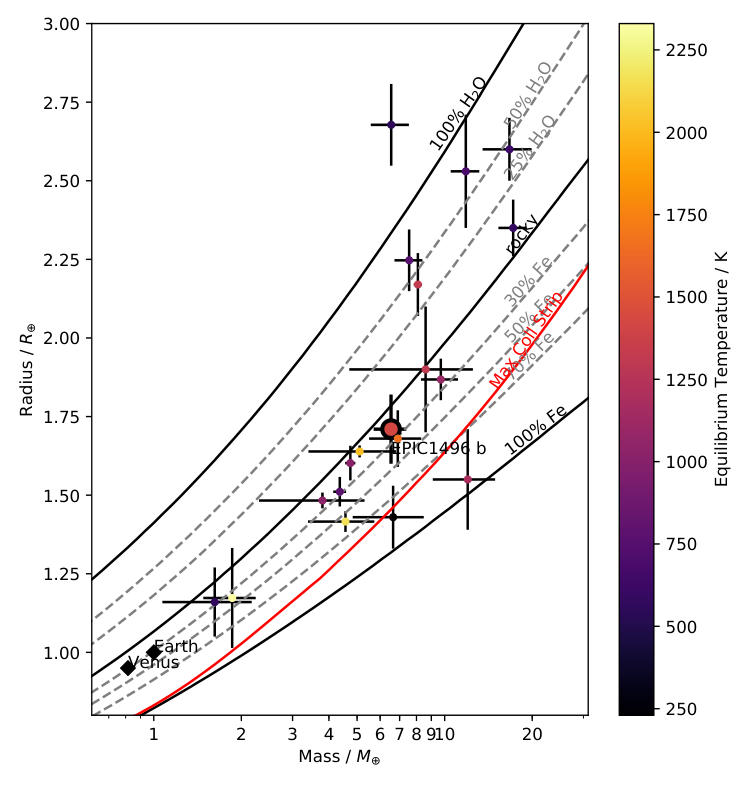
We performed a more detailed investigation of the composition of K2-265 b using the interior model of Brugger et al. (2017). This model considers planets made out of three differentiated layers: core (metals), mantle (rocks), and a liquid water envelope. Figure 7 shows the possible compositions of K2-265 b inferred from the 1- uncertainties on the planet’s mass and radius. By focusing on terrestrial compositions only (i.e. without any water), we show that the central mass and radius of the planet are best fitted with a rock mass fraction of 81%, consistently with other theoretical predictions. However, given the uncertainties on the fundamental parameters, the rmf remains poorly constrained, namely within the 44–100% range. If we assume that the stellar Fe/Si ratio (here ) can be used as a proxy for the bulk planetary value (Dorn et al. 2015; Brugger et al. 2017), this range is reduced to 60–83%. In the case of a water-rich K2-265 b, the model only allows us to derive an upper limit on the planet’s water mass fraction (wmf). Indeed, given the high equilibrium temperature of the planet ( K assuming an Earth-like albedo), water would be in the gaseous and supercritical phases, which are less dense than the liquid phase. From the uncertainties on the mass, radius, and bulk Fe/Si ratio of K2-265 b, we infer that this planet cannot present a wmf larger than 31%.
.
The California-Kepler Survey (CKS) measured precise stellar parameters of Kepler host stars using spectroscopic follow-up (Johnson et al. 2017), and refined the planetary radii to study the planet size distribution and planet occurrence rate (Fulton et al. 2017). The survey has revealed a bimodal distribution of small planet sizes. Planets tend to have radii of either or , with a deficit of planets at . The survey confirms the prediction by Owen & Wu (2013), whereby a gap in the planetary radius distribution exists as a consequence of atmospheric erosion by the photoevaporation mechanism. Alternatively, the core-powered mass loss mechanism could also drive the evaporation of small planets (Ginzburg et al. 2016; Ginzburg et al. 2018).
Due to its close proximity to the host star, the super-Earth K2-265 b is exposed to strong stellar irradiation. The planet’s gas envelope could be evaporated as a result. This process was observed in a number of systems (e.g. HD209458 b ; Vidal-Madjar et al. 2003, GJ 436 b; Ehrenreich et al. 2015). The present irradiance of the planet is , where and are the luminosity of the star and the Sun, is the Solar irradiance on Earth, and is the semi-major axis of the planet. The equilibrium temperature of the K2-265 b can be estimated using Equ. 1 of López-Morales & Seager (2007): , where f and are the reradiation factor and the Bond albedo of the planet. Assuming an Earth-like Bond albedo and that the incident radiation is redistributed around the atmosphere (i.e. ), the equilibrium temperature of K2-265 b is K.
Indeed, K2-265 b lies below the lower limit of the photoevaporation valley as shown in the 2D radius distribution plot in Figure 8. This implies that the planet could have been stripped bare due to photoevaporation, revealing its naked core. This atmospheric stripping process is presumed to have occurred in the first Myr since the birth of the planet when X-ray emission is saturated (Jackson et al. 2012), after which the X-ray emission decays. We estimated the total X-ray luminosity of K2-265 over its lifetime, , using the X-ray-age relation of Jackson et al. (2012). Using the results of section 3.5, we adopted a mean age of 6.32 Gyr for the host star. The X-ray-to-bolometric luminosity ratio in the saturated regime for a star is . The corresponding turn-off age is , where the decrease in X-ray emission follows a power law (). Over the lifetime of the star, ergs (assuming efficiency factor ) and K2-265 b is expected to have lost 2.7% of its mass under the constant-density assumption. K2-265 b has a predominantly rocky interior as shown in Figure 7. This indicates that the planet was likely formed inside the ice-line, and could have either migrated to its current orbital separation well before Myr or accreted its mass locally (Owen & Wu 2017).

K2-265 b is among the denser super-Earths below the photoevaporation gap. In addition to photoevaporation, giant impact between super-Earths could drive mass loss in the planetary atmosphere. Super-Earths are thought to have formed via accretion in gas discs, followed by migration and eccentricity damping due to their interactions with the gas disc (e.g. Lee & Chiang 2015), leading to densely packed planetary systems. As the gas disc disperses, secular perturbation between planets excites their eccentricity, triggering giant impacts between the bodies before the system becomes stable (Cossou et al. 2014). Two planets of comparable sizes could collide at a velocity beyond the surface escape velocity (Agnor & Asphaug 2004; Marcus et al. 2009). The impact could lead to a reduction in the planet envelope-to-core-mass ratio, hence an increase in the mean density and alteration of the bulk composition of the planet (Liu et al. 2015; Inamdar & Schlichting 2016).
Discoveries of super-Earths have shown a diversity of small planets in the mass-radius diagram. Precise RV and photometric measurements with an accuracy of a few percent are necessary to put strong constraints on the planetary mass and radius, and provide a precise bulk composition. The core composition of the planet can be derived as a result. In particular, the mass fraction of a planetary core can inform us of the formation and evolution history of the planet. K2-265 b has a precisely determined mass (13%) and radius (6%), and the composition of the planet is consistent with a rocky planet. Its small radius and short orbital period suggest that K2-265 b could have been photoevaporated to a bare rocky core. Its high rock-to-mass fraction implies a planet formation within the ice line. Studying planets with an exposed core could provide valuable insight to planet formation via the core accretion mechanism. The increasing sample of small planets will help distinguish planet origins, identify types of mass loss mechanism, and probe the efficiency of atmospheric evaporation processes.
Acknowledgements.
We thank the anonymous referee for the helpful comments which improved the manuscript. DJAB acknowledges support by the UK Space Agency. DJA gratefully acknowledges support from the STFC via an Ernest Rutherford Fellowship (ST/R00384X/1). This work was funded by FEDER - Fundo Europeu de Desenvolvimento Regional funds through the COMPETE 2020 - Programa Operacional Competitividade e Internacionalização (POCI), and by Portuguese funds through FCT - Fundação para a Ciência e a Tecnologia in the framework of the projects POCI-01-0145-FEDER-028953 and POCI-01-0145-FEDER-032113. N.S. and O.D. also acknowledge the support from FCT and FEDER through COMPETE2020 to grants UID/FIS/04434/2013 & POCI-01-0145-FEDER-007672, PTDC/FIS-AST/1526/2014 & POCI-01-0145-FEDER-016886 and PTDC/FIS-AST/7073/2014& POCI-01-0145-FEDER-016880. S.G.S acknowledge support from FCT through Investigador FCT contract nr. IF/00028/2014/CP1215/CT0002. SCCB also acknowledges support from FCT through Investigador FCT contracts IF/01312/2014/CP1215/CT0004. E.D.M. acknowledges the support by the Investigador FCT contract IF/00849/2015/CP1273/CT0003. RL has received funding from the European Union’s Horizon 2020 research and innovation programme under the Marie Skłodowska-Curie grant agreement n.664931. FF acknowledges support from PLATO ASI-INAF contract n.2015-019-R0. This research was made possible through the use of the AAVSO Photometric All-Sky Survey (APASS), funded by the Robert Martin Ayers Sciences Fund. This publication makes use of data products from the Two Micron All Sky Survey, which is a joint project of the University of Massachusetts and the Infrared Processing and Analysis Center/California Institute of Technology, funded by the National Aeronautics and Space Administration and the National Science Foundation. This publication makes use of data products from the Wide-field Infrared Survey Explorer, which is a joint project of the University of California, Los Angeles, and the Jet Propulsion Laboratory/California Institute of Technology, funded by the National Aeronautics and Space Administration. This research has made use of NASA’s Astrophysics Data System Bibliographic Services. This paper includes data collected by the K2 mission. Funding for the K2 mission is provided by the NASA Science Mission directorate. This research has made use of the Exoplanet Follow-up Observation Program website, which is operated by the California Institute of Technology, under contract with the National Aeronautics and Space Administration under the Exoplanet Exploration Program. This work has made use of data from the European Space Agency (ESA) mission Gaia (https://www.cosmos.esa.int/gaia), processed by the Gaia Data Processing and Analysis Consortium (DPAC, https://www.cosmos.esa.int/web/gaia/dpac/consortium). Funding for the DPAC has been provided by national institutions, in particular the institutions participating in the Gaia Multilateral Agreement.References
- Adibekyan et al. (2012) Adibekyan, V. Z., Sousa, S. G., Santos, N. C., et al. 2012, A&A, 545, A32
- Agnor & Asphaug (2004) Agnor, C. & Asphaug, E. 2004, ApJ, 613, L157
- Allard et al. (2012) Allard, F., Homeier, D., & Freytag, B. 2012, Philosophical Transactions of the Royal Society of London Series A, 370, 2765
- Andrae et al. (2018) Andrae, R., Fouesneau, M., Creevey, O., et al. 2018, ArXiv e-prints [arXiv:1804.09374]
- Armstrong et al. (2015a) Armstrong, D. J., Kirk, J., Lam, K. W. F., et al. 2015a, A&A, 579, A19
- Armstrong et al. (2015b) Armstrong, D. J., Santerne, A., Veras, D., et al. 2015b, A&A, 582, A33
- Baranne et al. (1996) Baranne, A., Queloz, D., Mayor, M., et al. 1996, A&AS, 119, 373
- Barnes (2010) Barnes, S. A. 2010, ApJ, 722, 222
- Barros et al. (2014) Barros, S. C. C., Almenara, J. M., Deleuil, M., et al. 2014, A&A, 569, A74
- Barros et al. (2015) Barros, S. C. C., Almenara, J. M., Demangeon, O., et al. 2015, MNRAS, 454, 4267
- Barros et al. (2016) Barros, S. C. C., Demangeon, O., & Deleuil, M. 2016, A&A, 594, A100
- Barros et al. (2017) Barros, S. C. C., Gosselin, H., Lillo-Box, J., et al. 2017, A&A, 608, A25
- Batalha (2014) Batalha, N. M. 2014, Proceedings of the National Academy of Science, 111, 12647
- Batalha et al. (2011) Batalha, N. M., Borucki, W. J., Bryson, S. T., et al. 2011, ApJ, 729, 27
- Batalha et al. (2013) Batalha, N. M., Rowe, J. F., Bryson, S. T., et al. 2013, ApJS, 204, 24
- Boisse et al. (2011) Boisse, I., Bouchy, F., Hébrard, G., et al. 2011, A&A, 528, A4
- Bonfils et al. (2013) Bonfils, X., Delfosse, X., Udry, S., et al. 2013, A&A, 549, A109
- Borucki et al. (2010) Borucki, W. J., Koch, D., Basri, G., et al. 2010, Science, 327, 977
- Borucki et al. (2011) Borucki, W. J., Koch, D. G., Basri, G., et al. 2011, ApJ, 736, 19
- Bouchy et al. (2001) Bouchy, F., Pepe, F., & Queloz, D. 2001, A&A, 374, 733
- Brugger et al. (2017) Brugger, B., Mousis, O., Deleuil, M., & Deschamps, F. 2017, ApJ, 850, 93
- Buchhave et al. (2016) Buchhave, L. A., Dressing, C. D., Dumusque, X., et al. 2016, AJ, 152, 160
- Charbonneau et al. (2009) Charbonneau, D., Berta, Z. K., Irwin, J., et al. 2009, Nature, 462, 891
- Claret & Bloemen (2011) Claret, A. & Bloemen, S. 2011, A&A, 529, A75
- Cossou et al. (2014) Cossou, C., Raymond, S. N., Hersant, F., & Pierens, A. 2014, A&A, 569, A56
- Cox (2000) Cox, A. N. 2000, Allen’s astrophysical quantities
- Crossfield et al. (2016) Crossfield, I. J. M., Ciardi, D. R., Petigura, E. A., et al. 2016, ApJS, 226, 7
- Cutri (2014) Cutri, R. M. e. 2014, VizieR Online Data Catalog, 2328
- Delgado Mena et al. (2014) Delgado Mena, E., Israelian, G., González Hernández, J. I., et al. 2014, A&A, 562, A92
- Delgado Mena et al. (2017) Delgado Mena, E., Tsantaki, M., Adibekyan, V. Z., et al. 2017, ArXiv e-prints [arXiv:1705.04349]
- Díaz et al. (2014) Díaz, R. F., Almenara, J. M., Santerne, A., et al. 2014, MNRAS, 441, 983
- Dittmann et al. (2017) Dittmann, J. A., Irwin, J. M., Charbonneau, D., et al. 2017, Nature, 544, 333
- Dorn et al. (2015) Dorn, C., Khan, A., Heng, K., et al. 2015, A&A, 577, A83
- Dotter et al. (2008) Dotter, A., Chaboyer, B., Jevremović, D., et al. 2008, ApJS, 178, 89
- Dressing & Charbonneau (2013) Dressing, C. D. & Charbonneau, D. 2013, ApJ, 767, 95
- Ecuvillon et al. (2004) Ecuvillon, A., Israelian, G., Santos, N. C., et al. 2004, A&A, 426, 619
- Ehrenreich et al. (2015) Ehrenreich, D., Bourrier, V., Wheatley, P. J., et al. 2015, Nature, 522, 459
- Fortney et al. (2007) Fortney, J. J., Marley, M. S., & Barnes, J. W. 2007, ApJ, 659, 1661
- Fulton et al. (2017) Fulton, B. J., Petigura, E. A., Howard, A. W., et al. 2017, AJ, 154, 109
- Gaia Collaboration et al. (2018) Gaia Collaboration, Brown, A. G. A., Vallenari, A., et al. 2018, ArXiv e-prints [arXiv:1804.09365]
- Gaia Collaboration et al. (2016) Gaia Collaboration, Prusti, T., de Bruijne, J. H. J., et al. 2016, A&A, 595, A1
- Ginzburg et al. (2016) Ginzburg, S., Schlichting, H. E., & Sari, R. 2016, ApJ, 825, 29
- Ginzburg et al. (2018) Ginzburg, S., Schlichting, H. E., & Sari, R. 2018, MNRAS, 476, 759
- Howard et al. (2012) Howard, A. W., Marcy, G. W., Bryson, S. T., et al. 2012, ApJS, 201, 15
- Howell et al. (2014) Howell, S. B., Sobeck, C., Haas, M., et al. 2014, PASP, 126, 398
- Inamdar & Schlichting (2016) Inamdar, N. K. & Schlichting, H. E. 2016, ApJ, 817, L13
- Jackson et al. (2012) Jackson, A. P., Davis, T. A., & Wheatley, P. J. 2012, MNRAS, 422, 2024
- Johnson et al. (2017) Johnson, J. A., Petigura, E. A., Fulton, B. J., et al. 2017, AJ, 154, 108
- Kipping (2010) Kipping, D. M. 2010, MNRAS, 408, 1758
- Koch et al. (2010) Koch, D. G., Borucki, W. J., Basri, G., et al. 2010, ApJ, 713, L79
- Lee & Chiang (2015) Lee, E. J. & Chiang, E. 2015, ApJ, 811, 41
- Ligi et al. (2018) Ligi, R., Demangeon, O., Barros, S., et al. 2018, ArXiv e-prints [arXiv:1809.03848]
- Lindegren et al. (2018) Lindegren, L., Hernandez, J., Bombrun, A., et al. 2018, ArXiv e-prints [arXiv:1804.09366]
- Lissauer et al. (2011) Lissauer, J. J., Fabrycky, D. C., Ford, E. B., et al. 2011, Nature, 470, 53
- Liu et al. (2015) Liu, S.-F., Hori, Y., Lin, D. N. C., & Asphaug, E. 2015, ApJ, 812, 164
- Lomb (1976) Lomb, N. R. 1976, Ap&SS, 39, 447
- Lopez & Fortney (2013) Lopez, E. D. & Fortney, J. J. 2013, ApJ, 776, 2
- López-Morales & Seager (2007) López-Morales, M. & Seager, S. 2007, ApJ, 667, L191
- Mamajek & Hillenbrand (2008) Mamajek, E. E. & Hillenbrand, L. A. 2008, ApJ, 687, 1264
- Marcus et al. (2010) Marcus, R. A., Sasselov, D., Hernquist, L., & Stewart, S. T. 2010, ApJ, 712, L73
- Marcus et al. (2009) Marcus, R. A., Stewart, S. T., Sasselov, D., & Hernquist, L. 2009, ApJ, 700, L118
- Mayo et al. (2018) Mayo, A. W., Vanderburg, A., Latham, D. W., et al. 2018, AJ, 155, 136
- Mayor et al. (2011) Mayor, M., Marmier, M., Lovis, C., et al. 2011, ArXiv e-prints [arXiv:1109.2497]
- Mayor et al. (2003) Mayor, M., Pepe, F., Queloz, D., et al. 2003, The Messenger, 114, 20
- McQuillan et al. (2013) McQuillan, A., Mazeh, T., & Aigrain, S. 2013, ApJ, 775, L11
- McQuillan et al. (2014) McQuillan, A., Mazeh, T., & Aigrain, S. 2014, ApJS, 211, 24
- Montet et al. (2015) Montet, B. T., Morton, T. D., Foreman-Mackey, D., et al. 2015, ApJ, 809, 25
- Munari et al. (2014) Munari, U., Henden, A., Frigo, A., et al. 2014, AJ, 148, 81
- Nissen (2015) Nissen, P. E. 2015, A&A, 579, A52
- Noyes et al. (1984) Noyes, R. W., Weiss, N. O., & Vaughan, A. H. 1984, ApJ, 287, 769
- Owen & Wu (2013) Owen, J. E. & Wu, Y. 2013, ApJ, 775, 105
- Owen & Wu (2017) Owen, J. E. & Wu, Y. 2017, ApJ, 847, 29
- Pepe et al. (2002) Pepe, F., Mayor, M., Rupprecht, G., et al. 2002, The Messenger, 110, 9
- Petigura et al. (2013) Petigura, E. A., Howard, A. W., & Marcy, G. W. 2013, Proceedings of the National Academy of Science, 110, 19273
- Pope et al. (2016) Pope, B. J. S., Parviainen, H., & Aigrain, S. 2016, MNRAS, 461, 3399
- Rogers (2015) Rogers, L. A. 2015, ApJ, 801, 41
- Santerne et al. (2018) Santerne, A., Brugger, B., Armstrong, D. J., et al. 2018, Nature Astronomy, 2, 393
- Santerne et al. (2015) Santerne, A., Díaz, R. F., Almenara, J.-M., et al. 2015, MNRAS, 451, 2337
- Santerne et al. (2016) Santerne, A., Hébrard, G., Lillo-Box, J., et al. 2016, ApJ, 824, 55
- Santos et al. (2015) Santos, N. C., Adibekyan, V., Mordasini, C., et al. 2015, A&A, 580, L13
- Scargle (1982) Scargle, J. D. 1982, ApJ, 263, 835
- Seager et al. (2007) Seager, S., Kuchner, M., Hier-Majumder, C. A., & Militzer, B. 2007, ApJ, 669, 1279
- Sinukoff et al. (2016) Sinukoff, E., Howard, A. W., Petigura, E. A., et al. 2016, ApJ, 827, 78
- Sneden (1973) Sneden, C. A. 1973, PhD thesis, The University of Texas at Austin.
- Sousa et al. (2015) Sousa, S. G., Santos, N. C., Adibekyan, V., Delgado-Mena, E., & Israelian, G. 2015, A&A, 577, A67
- Sousa et al. (2011) Sousa, S. G., Santos, N. C., Israelian, G., et al. 2011, A&A, 526, A99
- Sousa et al. (2008) Sousa, S. G., Santos, N. C., Mayor, M., et al. 2008, A&A, 487, 373
- Southworth (2008) Southworth, J. 2008, MNRAS, 386, 1644
- Stone (1989) Stone, R. C. 1989, AJ, 97, 1227
- Tucci Maia et al. (2016) Tucci Maia, M., Ramírez, I., Meléndez, J., et al. 2016, A&A, 590, A32
- Vanderburg & Johnson (2014) Vanderburg, A. & Johnson, J. A. 2014, PASP, 126, 948
- Vanderburg et al. (2016) Vanderburg, A., Latham, D. W., Buchhave, L. A., et al. 2016, ApJS, 222, 14
- Vanderburg et al. (2015) Vanderburg, A., Montet, B. T., Johnson, J. A., et al. 2015, ApJ, 800, 59
- Vidal-Madjar et al. (2003) Vidal-Madjar, A., Lecavelier des Etangs, A., Désert, J.-M., et al. 2003, Nature, 422, 143
- Vigan et al. (2016) Vigan, A., Bonnefoy, M., Ginski, C., et al. 2016, A&A, 587, A55
- Vigan et al. (2010) Vigan, A., Moutou, C., Langlois, M., et al. 2010, MNRAS, 407, 71
- Weiss & Marcy (2014) Weiss, L. M. & Marcy, G. W. 2014, ApJ, 783, L6
- Zeng & Sasselov (2013) Zeng, L. & Sasselov, D. 2013, PASP, 125, 227
- Zeng et al. (2016) Zeng, L., Sasselov, D. D., & Jacobsen, S. B. 2016, ApJ, 819, 127
- Zurlo et al. (2014) Zurlo, A., Vigan, A., Mesa, D., et al. 2014, A&A, 572, A85
Appendix A Supplementary Tables and Figures

| Instrument | Date | Sep. | Pos. ang. | ||
|---|---|---|---|---|---|
| (mas) | (mas) | (mas) | (deg) | ||
| Keck/NIRC2 | 2015-08-04 | -910 5 | -363 5 | 979 5 | 248.27 0.29 |
| VLT/SPHERE | 2015-08-04 | -906 1 | -368 1 | 978 1 | 247.87 0.20 |
| VLT/SPHERE | 2017-08-30 | -903 1 | -365 1 | 975 1 | 247.99 0.01 |
| Element | Abundance | Lines number |
|---|---|---|
| X/H | [dex] | |
| C 1 | 2 | |
| O 1 | 2 | |
| Na 1 | 2 | |
| Mg 1 | 3 | |
| Al 1 | 2 | |
| Si 1 | 11 | |
| S 1 | 2 | |
| Ca 1 | 9 | |
| Sc 1 | 3 | |
| Sc 2 | 6 | |
| Ti 1 | 18 | |
| Ti 2 | 5 | |
| V 1 | 6 | |
| Cr 1 | 17 | |
| Mn 1 | 5 | |
| Co 1 | 7 | |
| Ni 1 | 40 | |
| Cu 1 | 4 | |
| Zn 1 | 3 | |
| Sr 1 | 1 | |
| Y 2 | 6 | |
| Zr 2 | 4 | |
| Ba 2 | 3 | |
| Ce 2 | 4 | |
| Nd 2 | 2 | |
| A(Li 1)∗ | 1 | |
| ∗A(Li) = log[N(Li)/N(H)] + 12 | ||
| Time | RV | RV | FWHM | FWHM | BIS | BIS | SMW | SMW | S/N |
|---|---|---|---|---|---|---|---|---|---|
| BJD | [km s-1] | [m s-1] | [km s-1] | [m s-1] | [m s-1] | [m s-1] | |||
| 57690.54527 | -18.19493 | 2.01 | 6.9428 | 4.0 | -27.1 | 4.0 | 0.1820 | 0.0064 | 46.8 |
| 57690.65420 | -18.19306 | 1.70 | 6.9393 | 3.4 | -24.5 | 3.4 | 0.1826 | 0.0056 | 57.3 |
| 57691.52542 | -18.18932 | 1.84 | 6.9423 | 3.7 | -27.3 | 3.7 | 0.1755 | 0.0056 | 51.0 |
| 57691.64089 | -18.18784 | 1.57 | 6.9380 | 3.1 | -19.0 | 3.1 | 0.1789 | 0.0052 | 62.8 |
| 57692.54337 | -18.19043 | 1.82 | 6.9336 | 3.6 | -17.0 | 3.6 | 0.1799 | 0.0057 | 52.2 |
| 57692.66890 | -18.19007 | 2.03 | 6.9400 | 4.1 | -18.4 | 4.1 | 0.1868 | 0.0082 | 48.1 |
| 57694.55555 | -18.18570 | 1.90 | 6.9404 | 3.8 | -30.9 | 3.8 | 0.1873 | 0.0061 | 50.0 |
| 57694.65367 | -18.18799 | 1.89 | 6.9472 | 3.8 | -17.4 | 3.8 | 0.1825 | 0.0071 | 51.6 |
| 57695.53842 | -18.19169 | 2.29 | 6.9375 | 4.6 | -34.0 | 4.6 | 0.1877 | 0.0077 | 40.8 |
| 57695.55993 | -18.19412 | 2.09 | 6.9479 | 4.2 | -24.2 | 4.2 | 0.1730 | 0.0065 | 44.5 |
| 57696.54203 | -18.19052 | 2.05 | 6.9560 | 4.1 | -26.0 | 4.1 | 0.1857 | 0.0068 | 45.8 |
| 57696.67629 | -18.19411 | 1.94 | 6.9507 | 3.9 | -22.7 | 3.9 | 0.1817 | 0.0075 | 50.1 |
| 57697.56269 | -18.19541 | 1.90 | 6.9536 | 3.8 | -29.4 | 3.8 | 0.1788 | 0.0061 | 49.7 |
| 57697.64405 | -18.19883 | 1.74 | 6.9470 | 3.5 | -26.9 | 3.5 | 0.1855 | 0.0058 | 55.5 |
| 57699.51415 | -18.18805 | 1.53 | 6.9476 | 3.1 | -24.6 | 3.1 | 0.2188 | 0.0041 | 62.7 |
| 57699.56041 | -18.18795 | 1.56 | 6.9584 | 3.1 | -18.3 | 3.1 | 0.2205 | 0.0048 | 62.6 |
| 57701.53183 | -18.18327 | 2.03 | 6.9532 | 4.1 | -26.0 | 4.1 | 0.2197 | 0.0061 | 45.9 |
| 57701.57985 | -18.18358 | 2.01 | 6.9494 | 4.0 | -26.0 | 4.0 | 0.2343 | 0.0061 | 46.5 |
| 57703.53660 | -18.18968 | 1.74 | 6.9375 | 3.5 | -15.2 | 3.5 | 0.2164 | 0.0054 | 55.2 |
| 57703.57238 | -18.18313 | 1.78 | 6.9565 | 3.6 | -15.9 | 3.6 | 0.2190 | 0.0055 | 53.8 |
| 57705.53138 | -18.19312 | 1.53 | 6.9390 | 3.1 | -12.6 | 3.1 | 0.2031 | 0.0045 | 64.9 |
| 57705.57766 | -18.19513 | 1.76 | 6.9337 | 3.5 | -16.9 | 3.5 | 0.2142 | 0.0060 | 55.6 |
| 57714.60057 | -18.19074 | 2.33 | 6.9600 | 4.7 | -13.1 | 4.7 | 0.2277 | 0.0086 | 41.2 |
| 57714.62010 | -18.19333 | 2.37 | 6.9489 | 4.7 | -12.6 | 4.7 | 0.2225 | 0.0099 | 41.4 |
| 57717.55993 | -18.19042 | 2.01 | 6.9418 | 4.0 | -17.8 | 4.0 | 0.1746 | 0.0073 | 48.1 |
| 57717.58112 | -18.18483 | 2.13 | 6.9487 | 4.3 | -17.2 | 4.3 | 0.1940 | 0.0079 | 45.2 |
| 57718.53008 | -18.19030 | 1.78 | 6.9488 | 3.6 | -17.7 | 3.6 | 0.1990 | 0.0061 | 54.1 |
| 57718.55149 | -18.18923 | 1.73 | 6.9507 | 3.5 | -12.9 | 3.5 | 0.2019 | 0.0060 | 56.2 |
| 57719.55290 | -18.19238 | 1.71 | 6.9511 | 3.4 | -22.8 | 3.4 | 0.1884 | 0.0056 | 56.5 |
| 57719.57368 | -18.19477 | 1.71 | 6.9425 | 3.4 | -18.4 | 3.4 | 0.1994 | 0.0057 | 56.7 |
| 57720.53108 | -18.18721 | 1.45 | 6.9469 | 2.9 | -14.2 | 2.9 | 0.1922 | 0.0046 | 70.4 |
| 57720.55102 | -18.18671 | 1.52 | 6.9397 | 3.0 | -17.1 | 3.0 | 0.1968 | 0.0051 | 65.7 |
| 57721.53077 | -18.19020 | 2.01 | 6.9556 | 4.0 | -24.1 | 4.0 | 0.1938 | 0.0070 | 47.5 |
| 57721.55300 | -18.18965 | 2.09 | 6.9408 | 4.2 | -14.9 | 4.2 | 0.1838 | 0.0076 | 45.7 |
| 57935.79544 | -18.17258 | 2.34 | 6.9898 | 4.7 | -7.0 | 4.7 | 0.2700 | 0.0091 | 42.0 |
| 57935.81684 | -18.17136 | 2.21 | 6.9761 | 4.4 | -5.1 | 4.4 | 0.2564 | 0.0084 | 44.2 |
| 57936.84590 | -18.17932 | 2.48 | 6.9803 | 5.0 | -15.5 | 5.0 | 0.2820 | 0.0100 | 39.7 |
| 57936.86711 | -18.18014 | 2.53 | 6.9722 | 5.1 | 1.8 | 5.1 | 0.2668 | 0.0104 | 39.1 |
| 57937.77515 | -18.17689 | 2.58 | 6.9604 | 5.2 | -6.9 | 5.2 | 0.2415 | 0.0105 | 38.3 |
| 57937.82206 | -18.17986 | 2.30 | 6.9765 | 4.6 | -15.1 | 4.6 | 0.2444 | 0.0088 | 42.4 |
| 57942.77873 | -18.18570 | 1.58 | 6.9310 | 3.2 | -19.1 | 3.2 | 0.2124 | 0.0046 | 61.4 |
| 57942.88776 | -18.19012 | 1.65 | 6.9373 | 3.3 | -15.1 | 3.3 | 0.2270 | 0.0066 | 61.1 |
| 57943.75116 | -18.18923 | 1.62 | 6.9337 | 3.2 | -13.2 | 3.2 | 0.1961 | 0.0048 | 60.4 |
| 57943.86160 | -18.19289 | 2.46 | 6.9371 | 4.9 | -21.2 | 4.9 | 0.1863 | 0.0097 | 39.7 |
| 57944.77832 | -18.19228 | 2.24 | 6.9244 | 4.5 | -15.5 | 4.5 | 0.1864 | 0.0082 | 42.9 |
| 57944.86188 | -18.19112 | 1.99 | 6.9344 | 4.0 | -25.0 | 4.0 | 0.1829 | 0.0075 | 48.7 |
| 57945.75844 | -18.18714 | 1.79 | 6.9247 | 3.6 | -23.8 | 3.6 | 0.1759 | 0.0057 | 53.7 |
| 57946.77897 | -18.19034 | 2.30 | 6.9292 | 4.6 | -25.4 | 4.6 | 0.1791 | 0.0080 | 42.0 |
| 57948.80722 | -18.18963 | 2.00 | 6.9241 | 4.0 | -25.8 | 4.0 | 0.1690 | 0.0069 | 48.4 |
| 57948.86573 | -18.19051 | 2.09 | 6.9274 | 4.2 | -21.6 | 4.2 | 0.1760 | 0.0080 | 46.5 |
| 57949.84184 | -18.18010 | 5.61 | 6.9040 | 11.2 | -11.5 | 11.2 | 0.1322 | 0.0280 | 20.3 |
| 57951.76491 | -18.19084 | 4.40 | 6.9380 | 8.8 | -23.9 | 8.8 | 0.2072 | 0.0226 | 24.4 |
| 57951.85922 | -18.17271 | 3.38 | 6.9374 | 6.8 | -17.4 | 6.8 | 0.1802 | 0.0169 | 30.3 |
| 57952.73957 | -18.17978 | 3.26 | 6.9507 | 6.5 | -13.5 | 6.5 | 0.1720 | 0.0148 | 31.2 |
| 57952.86046 | -18.17574 | 2.49 | 6.9466 | 5.0 | -27.4 | 5.0 | 0.1881 | 0.0111 | 39.7 |
| 57953.85555 | -18.18618 | 2.46 | 6.9581 | 4.9 | -19.0 | 4.9 | 0.1945 | 0.0105 | 40.1 |
| 57954.82099 | -18.17750 | 3.16 | 6.9479 | 6.3 | -23.7 | 6.3 | 0.1541 | 0.0150 | 32.5 |
| 57955.75309 | -18.17132 | 2.30 | 6.9634 | 4.6 | -16.6 | 4.6 | 0.1838 | 0.0080 | 41.8 |
| 57955.91602 | -18.17448 | 1.72 | 6.9752 | 3.4 | -26.9 | 3.4 | 0.1939 | 0.0077 | 59.6 |
| 57956.72888 | -18.17041 | 2.32 | 6.9676 | 4.6 | -25.0 | 4.6 | 0.2022 | 0.0082 | 41.8 |
| 57956.91804 | -18.17142 | 2.42 | 6.9667 | 4.8 | -33.5 | 4.8 | 0.2255 | 0.0106 | 41.0 |
| 57957.89416 | -18.17995 | 4.32 | 6.9690 | 8.6 | -10.7 | 8.6 | 0.1634 | 0.0218 | 25.0 |
| 57959.78548 | -18.17701 | 2.51 | 6.9612 | 5.0 | -15.7 | 5.0 | 0.2194 | 0.0103 | 39.4 |
| 57959.90585 | -18.17966 | 1.91 | 6.9555 | 3.8 | -16.3 | 3.8 | 0.2075 | 0.0084 | 52.1 |
| 57960.74725 | -18.18476 | 2.68 | 6.9651 | 5.4 | -20.1 | 5.4 | 0.2090 | 0.0104 | 36.9 |
| 57960.84628 | -18.18490 | 2.65 | 6.9605 | 5.3 | -12.9 | 5.3 | 0.1981 | 0.0108 | 37.4 |
| 57961.76442 | -18.17957 | 2.22 | 6.9582 | 4.4 | -7.1 | 4.4 | 0.2149 | 0.0087 | 44.4 |
| 57961.83425 | -18.18436 | 2.41 | 6.9526 | 4.8 | -16.7 | 4.8 | 0.2094 | 0.0171 | 43.3 |
| 57962.78393 | -18.17748 | 1.96 | 6.9541 | 3.9 | -2.2 | 3.9 | 0.2119 | 0.0081 | 51.1 |
| 57962.87271 | -18.19164 | 5.55 | 6.9251 | 11.1 | -18.0 | 11.1 | 0.2266 | 0.0438 | 21.7 |
| 57964.74231 | -18.17793 | 1.84 | 6.9650 | 3.7 | -11.6 | 3.7 | 0.2149 | 0.0061 | 52.7 |
| 57964.83225 | -18.18182 | 1.94 | 6.9492 | 3.9 | -20.0 | 3.9 | 0.2078 | 0.0089 | 51.7 |
| 57965.73570 | -18.19438 | 5.34 | 6.9277 | 10.7 | -25.5 | 10.7 | 0.1945 | 0.0308 | 21.4 |
| 57965.83742 | -18.18131 | 5.94 | 6.9409 | 11.9 | -8.8 | 11.9 | 0.2740 | 0.0440 | 20.4 |
| 57993.66968 | -18.18228 | 2.03 | 6.9482 | 4.1 | -22.7 | 4.1 | 0.2104 | 0.0075 | 47.0 |
| 57993.78491 | -18.17993 | 2.08 | 6.9523 | 4.2 | -18.3 | 4.2 | 0.1954 | 0.0086 | 46.3 |
| 57993.84799 | -18.18314 | 1.83 | 6.9520 | 3.7 | -27.1 | 3.7 | 0.1934 | 0.0088 | 53.9 |
| 57994.63060 | -18.17385 | 1.98 | 6.9446 | 4.0 | -22.7 | 4.0 | 0.1980 | 0.0070 | 47.8 |
| 57994.74383 | -18.17639 | 2.22 | 6.9466 | 4.4 | -16.1 | 4.4 | 0.1864 | 0.0091 | 43.3 |
| 57994.82005 | -18.17586 | 2.19 | 6.9553 | 4.4 | -23.9 | 4.4 | 0.2004 | 0.0102 | 44.6 |
| 57995.63098 | -18.17764 | 3.46 | 6.9558 | 6.9 | -23.8 | 6.9 | 0.1701 | 0.0174 | 29.9 |
| 57998.62754 | -18.19046 | 1.56 | 6.9459 | 3.1 | -15.7 | 3.1 | 0.1987 | 0.0046 | 61.3 |
| 57998.71879 | -18.19124 | 2.02 | 6.9506 | 4.0 | -14.9 | 4.0 | 0.1797 | 0.0087 | 48.3 |
| 57998.81073 | -18.18741 | 2.21 | 6.9488 | 4.4 | -17.8 | 4.4 | 0.1645 | 0.0116 | 45.0 |
| 58008.66469 | -18.18777 | 3.48 | 6.9314 | 7.0 | -7.3 | 7.0 | 0.1958 | 0.0153 | 29.0 |
| 58010.65231 | -18.19970 | 2.19 | 6.9277 | 4.4 | -28.0 | 4.4 | 0.1689 | 0.0085 | 43.3 |
| 58010.77942 | -18.19305 | 2.25 | 6.9234 | 4.5 | -26.8 | 4.5 | 0.1921 | 0.0107 | 43.3 |
| 58010.83344 | -18.19911 | 2.07 | 6.9391 | 4.1 | -28.7 | 4.1 | 0.1985 | 0.0115 | 47.9 |
| 58011.68577 | -18.18190 | 2.40 | 6.9283 | 4.8 | -9.4 | 4.8 | 0.1728 | 0.0105 | 40.2 |
| 58011.77789 | -18.18417 | 2.23 | 6.9321 | 4.5 | -15.3 | 4.5 | 0.1739 | 0.0104 | 43.6 |
| 58011.83205 | -18.18652 | 2.60 | 6.9261 | 5.2 | -37.8 | 5.2 | 0.1888 | 0.0150 | 38.6 |
| 58012.67262 | -18.18860 | 2.91 | 6.9347 | 5.8 | -29.1 | 5.8 | 0.1680 | 0.0137 | 34.0 |
| 58012.75336 | -18.19386 | 2.31 | 6.9312 | 4.6 | -35.4 | 4.6 | 0.1780 | 0.0106 | 42.0 |
| 58012.82174 | -18.18669 | 2.43 | 6.9230 | 4.9 | -17.5 | 4.9 | 0.1579 | 0.0132 | 40.9 |
| 58013.67492 | -18.18197 | 3.38 | 6.9334 | 6.8 | -28.1 | 6.8 | 0.1733 | 0.0158 | 30.1 |
| 58013.74342 | -18.18162 | 2.52 | 6.9295 | 5.0 | -21.7 | 5.0 | 0.1862 | 0.0109 | 38.5 |
| 58013.81433 | -18.18331 | 2.17 | 6.9467 | 4.3 | -31.5 | 4.3 | 0.1964 | 0.0106 | 45.2 |
| 58014.68555 | -18.18273 | 2.62 | 6.9207 | 5.2 | -26.3 | 5.2 | 0.2481 | 0.0102 | 37.1 |
| 58014.77534 | -18.18936 | 2.77 | 6.9302 | 5.5 | -28.6 | 5.5 | 0.1661 | 0.0130 | 36.0 |
| 58018.63224 | -18.18640 | 2.33 | 6.9479 | 4.7 | -28.0 | 4.7 | 0.1890 | 0.0095 | 40.9 |
| 58018.72534 | -18.18438 | 2.52 | 6.9262 | 5.0 | -23.1 | 5.0 | 0.1978 | 0.0108 | 38.2 |
| 58019.62715 | -18.19033 | 1.99 | 6.9432 | 4.0 | -20.6 | 4.0 | 0.1888 | 0.0077 | 47.8 |
| 58019.72843 | -18.19547 | 1.92 | 6.9260 | 3.8 | -25.9 | 3.8 | 0.1963 | 0.0080 | 49.9 |
| 58020.66431 | -18.18766 | 3.01 | 6.9468 | 6.0 | -5.8 | 6.0 | 0.1870 | 0.0121 | 32.5 |
| 58020.75915 | -18.18656 | 2.21 | 6.9431 | 4.4 | -19.1 | 4.4 | 0.1977 | 0.0099 | 43.6 |
| 58021.55154 | -18.17666 | 2.55 | 6.9344 | 5.1 | -19.9 | 5.1 | 0.2109 | 0.0103 | 37.6 |
| 58021.66021 | -18.18003 | 3.07 | 6.9414 | 6.1 | -35.5 | 6.1 | 0.2225 | 0.0132 | 32.3 |
| 58021.75738 | -18.18448 | 2.24 | 6.9325 | 4.5 | -15.9 | 4.5 | 0.1845 | 0.0100 | 43.1 |
| 58022.53363 | -18.18830 | 2.59 | 6.9472 | 5.2 | -24.9 | 5.2 | 0.1947 | 0.0103 | 37.1 |
| 58022.59935 | -18.18210 | 3.26 | 6.9427 | 6.5 | -17.1 | 6.5 | 0.1937 | 0.0128 | 30.2 |
| 58022.74556 | -18.19200 | 2.80 | 6.9414 | 5.6 | -22.3 | 5.6 | 0.2040 | 0.0124 | 35.0 |
| 58023.53440 | -18.17930 | 1.81 | 6.9489 | 3.6 | -32.0 | 3.6 | 0.2030 | 0.0058 | 51.1 |
| 58023.63020 | -18.17708 | 2.62 | 6.9523 | 5.2 | -19.1 | 5.2 | 0.1963 | 0.0106 | 36.7 |
| 58023.75632 | -18.18220 | 2.00 | 6.9325 | 4.0 | -24.1 | 4.0 | 0.1824 | 0.0092 | 48.3 |
| 58025.54957 | -18.17300 | 1.67 | 6.9443 | 3.3 | -17.9 | 3.3 | 0.2031 | 0.0055 | 56.1 |
| 58025.64932 | -18.17642 | 1.82 | 6.9560 | 3.6 | -19.6 | 3.6 | 0.1990 | 0.0074 | 52.8 |
| 58025.70429 | -18.17085 | 1.93 | 6.9569 | 3.9 | -4.2 | 3.9 | 0.2057 | 0.0089 | 50.3 |
| 58026.55716 | -18.16496 | 4.02 | 6.9580 | 8.0 | -8.4 | 8.0 | 0.2396 | 0.0170 | 25.7 |
| 58026.65617 | -18.17836 | 2.73 | 6.9569 | 5.5 | -22.0 | 5.5 | 0.2263 | 0.0112 | 35.7 |
| 58026.74871 | -18.18277 | 2.88 | 6.9711 | 5.8 | -22.1 | 5.8 | 0.1771 | 0.0154 | 35.2 |
| 58027.56593 | -18.15614 | 5.14 | 6.9831 | 10.3 | -11.8 | 10.3 | 0.2023 | 0.0274 | 21.8 |
| 58027.67900 | -18.16790 | 4.30 | 7.0036 | 8.6 | -8.0 | 8.6 | 0.1720 | 0.0246 | 25.4 |
| 58027.74799 | -18.15559 | 5.45 | 6.9669 | 10.9 | 28.2 | 10.9 | 0.1827 | 0.0322 | 21.1 |
| 58041.54788 | -18.19556 | 2.00 | 6.9314 | 4.0 | -31.2 | 4.0 | 0.1730 | 0.0067 | 47.1 |
| 58043.56762 | -18.18878 | 1.35 | 6.9287 | 2.7 | -24.3 | 2.7 | 0.2094 | 0.0039 | 73.6 |
| 58043.72519 | -18.18693 | 1.89 | 6.9299 | 3.8 | -25.9 | 3.8 | 0.2145 | 0.0086 | 52.1 |
| 58052.55248 | -18.18881 | 1.46 | 6.9380 | 2.9 | -22.7 | 2.9 | 0.2180 | 0.0046 | 66.9 |
| 58052.61595 | -18.19051 | 1.95 | 6.9391 | 3.9 | -27.6 | 3.9 | 0.2350 | 0.0085 | 50.3 |
| 58053.56897 | -18.18273 | 1.70 | 6.9377 | 3.4 | -27.6 | 3.4 | 0.2239 | 0.0060 | 56.8 |
| 58053.64640 | -18.18326 | 1.80 | 6.9436 | 3.6 | -23.4 | 3.6 | 0.2202 | 0.0074 | 54.6 |
| 58054.52491 | -18.18453 | 2.44 | 6.9497 | 4.9 | -36.6 | 4.9 | 0.2112 | 0.0083 | 39.1 |
| 58054.67331 | -18.18235 | 2.09 | 6.9612 | 4.2 | -21.0 | 4.2 | 0.2261 | 0.0086 | 46.9 |
| 58056.53663 | -18.18039 | 1.35 | 6.9497 | 2.7 | -23.1 | 2.7 | 0.2132 | 0.0039 | 74.8 |
| 58056.62290 | -18.18640 | 1.60 | 6.9600 | 3.2 | -33.6 | 3.2 | 0.2198 | 0.0064 | 62.6 |
| 58057.53537 | -18.18602 | 1.32 | 6.9511 | 2.6 | -28.4 | 2.6 | 0.2202 | 0.0038 | 76.5 |
| 58057.59482 | -18.18711 | 1.41 | 6.9528 | 2.8 | -29.3 | 2.8 | 0.2291 | 0.0049 | 71.7 |
| 58068.58875 | -18.18136 | 1.63 | 6.9330 | 3.3 | -14.5 | 3.3 | 0.1845 | 0.0055 | 59.0 |
| 58069.65402 | -18.19329 | 1.90 | 6.9399 | 3.8 | -17.5 | 3.8 | 0.1783 | 0.0062 | 49.6 |
| 58070.66278 | -18.19205 | 1.93 | 6.9408 | 3.9 | -20.7 | 3.9 | 0.1868 | 0.0086 | 50.8 |
| 58071.54887 | -18.18911 | 1.69 | 6.9187 | 3.4 | -23.1 | 3.4 | 0.1924 | 0.0061 | 56.8 |
| 58074.55346 | -18.18790 | 1.55 | 6.9236 | 3.1 | -18.4 | 3.1 | 0.1788 | 0.0060 | 62.4 |
| 58075.53852 | -18.18124 | 1.76 | 6.9243 | 3.5 | -18.9 | 3.5 | 0.1630 | 0.0069 | 54.5 |
| 58077.54947 | -18.18492 | 1.60 | 6.9297 | 3.2 | -23.9 | 3.2 | 0.1872 | 0.0063 | 61.9 |
| 58079.61835 | -18.19371 | 1.94 | 6.9281 | 3.9 | -21.6 | 3.9 | 0.1803 | 0.0084 | 49.5 |
| Parameter | Prior | Posterior | |
|---|---|---|---|
| Dartmouth | PARSEC | ||
| (adopted) | |||
| Stellar Parameters | |||
| Effective temperature Teff [K] | |||
| Surface gravity log g [cgs] | |||
| Iron abundance [Fe/H] [dex] | |||
| Distance to Earth [pc] | |||
| Interstellar extinction [mag] | |||
| Systemic radial velocity [km s-1] | |||
| Linear limb-darkening coefficient | (derived) | ||
| Quadratic limb-darkening coefficient | (derived) | ||
| Stellar density | (derived) | ||
| Stellar mass M⋆ [] | (derived) | ||
| Stellar radius R⋆ [] | (derived) | ||
| Stellar age [Gyr] | (derived) | ||
| Planet b Parameters | |||
| Orbital Period [d] | |||
| Transit epoch [BJD - 2456000] | |||
| Radial velocity semi-amplitude [m s-1] | |||
| Orbital inclination [∘] | |||
| Planet-to-star radius ratio | |||
| Orbital eccentricity | |||
| Argument of periastron [∘] | |||
| System scale | (derived) | ||
| Impact parameter | (derived) | ||
| Transit duration T14 [h] | (derived) | ||
| Semi-major axis [AU] | (derived) | ||
| Planet mass Mp [] | (derived) | ||
| Planet radius Rp [] | (derived) | ||
| Planet bulk density [g cm-3] | (derived) | ||
| Gaussian Process Hyperparameters | |||
| [m s-1] | |||
| [d] | |||
| [d] | |||
| Instrument-related Parameters | |||
| HARPS jitter [m s-1] | |||
| K2 contamination [%] | |||
| K2 jitter [ppm] | |||
| K2 out-of-transit flux | |||
| SED jitter [mag] | |||
| Notes: | |||
| : normal distribution with mean and width | |||
| : uniform distribution between and | |||
| : normal distribution with mean and width multiplied with a uniform distribution between and | |||
| : sine distribution between and | |||
| : Beta distribution with parameters and | |||