Modeling non-linear spectral domain dependence using copulas with applications to rat local field potentials

Brain stroke occurs when blood circulation in one of the cerebral blood vessels is abnormally weak, and in such case, leads to death of the cells.. Brain stroke has been studied for years by biologists and neurologists. Studying this disorder from the perspective of the changes in the brain’s electrical activities among different regions has yielded many clinically important results: these changes are so important that often they do irreversible damages to patients and incur extravagant costs to society (e.g., high medical expenses and low quality of patients’ lives). In order to reduce these societal costs, neuroscientists study the behavior of the cortex activity by inducing stroke in rats. Due to ethical considerations, stroke experiments are conducted mostly only on rats. This paper is based on an experimental setup designed to induce stroke in a rat and to study the electrical oscillations among different regions in his brain. Using the copula information, we developed methods for assessing and analyzing dependence between the rat’s brain regions. Our work is in collaboration with neuroscientists from University of California at Irvine (co-author Frostig and student Wann [39]) who mechanically induced brain stroke in the rats by clamping a brain artery and recorded the brain activity on $32$ microelectrodes (or channels) before and after the stroke. Figure 1 shows, for one of the analyzed rats, how the data act differently in the pre-stroke phase (first $5$ minutes or first $300$ epochs) versus in the post-stroke phase (last $5$ minutes or last $300$ epochs). The detailed setup is described in Section 4.

One goal is to analyze the changes in the dependence between some channels for all frequency bands by using flexible models. Most analyses use coherence or correlation which are simple to implement but they are severely limited because they capture only linear dependence structures. Thus, we present an innovative methodology based on the notion of copula function to capture the complexity of the dependence and by comparing two (or more) copulas. Moreover, we assess whether or not the dependence between pairs of epochs changes across ($1$-second) epochs of the entire recording period. From the recorded electrical activity during the laboratory experiment, the impact of brain stroke is observable for most microelectrodes on almost all frequency bands; and the effect of the stroke on brain signals appear to last throughout the entire post-stroke recording (see Appendix 15). Our contributions in this paper are the following. First, we present an algorithm to help recognize which epoch(s) exhibit changes in the dependence structure of the brain signals. This recognition of a changepoint is key to understanding the biological mechanisms occurring in the time window between the onset of the stroke and the moment where significant changes occur. Second, we present a method to assess if the dependence structure during pre-stroke differs from the one from post-stroke. This assessment is crucial to understand if this channel will be impacted by the stroke. This method is also used later to compare the dependence structure among two different channels for a given frequency band.

In the literature, many studies investigated changes in dependence for brain channels (in electroencephalograms) defined in the spectral domain. Among them, we highlight Ombao et al. [31], Fiecas and Ombao [15], Long et al. [28], Purdon et al. [34], Nunez et al. [30] and Gotman [18]. However, the primary limitation of these studies is that they look only into the linear dependence between signals. Thus, they could miss potential complex (or non-linear) dependence structure between signals. Most methods reported explored the problem of detecting one (or many) changepoint moment(s) (e.g., within an epoch). A major approach is based on segmentation of the series in order to assess a possible discrepancy between these segments: on either a change in mean or a difference in the correlation structure. Many authors considered the segmentation: e.g., Adak [2] with binary trees and windowed spectra to adaptively partition data; Ombao et al. [32] derive a segmentation by selecting the best localized basis from the SLEX (smooth local exponential) library. Another example is the estimation of a penalized minimum contrast (Lavielle [26]). Its principle has two steps. In the first step, a contrast function is computed over a segments of a time period (or a sequence defined in the frequency domain - see Lavielle et al. [27]). The changepoints are then selected to be a solution to the minimization problem. Another example of that segmentation is based on probabilistic pruning methods. The principle of pruning is to predict the probability that a segment belongs to a stationary process rather than its likelihood. This method has been well studied by James and Matteson [22] and Kifer et al. [25]. Another approach presented by Davis et al. [10] is the Auto-PARM: it consists in fitting multiple auto-regressive (AR) functions to segments of time. But fitting the AR model could be subject to model misspecification. The third kind of methods for detecting changepoints is based on hypothesis tests. Dette and Paparoditis [12] and Dette and Hildebrandt [11] proposed an approach to test the equality of spectrum between two successive segments. This idea iis interesting but it does not take into account the nature and the structure of the dependence between these successive segments.

The use of the joint cumulative distribution functions with brain signals has also been explored to study dependence between random variables in general. These functions, namely copula models, have the main advantage to represent the dependence as functions that provide the information of both ”strength” and ”structure” of the relation between two variables. For example, in Figure 1, for the three cases, it is obvious that the dependence pattern between succeeding epochs during pre-stroke (first $300$ epochs) and the one during post-stroke (last $300$ epochs) are different and that the dependence structure from epoch $300$ to epoch $400$ is not the same than the one between epoch $500$ and epoch $600$. These particularities in dependence structure will be fully detected with a copula under a right specification. Iyengar et al. [21] used it to quantify synchronicity between multiples electroencephalographic (EEG) signals. Dauwels et al. [9] used copulas in their attempt to design brain network. Ince et al. [20] presented a framework to assess dependence for neuroimaging data based on the gaussian copula. Even if all of these approaches presented a copula-based framework for brain signals data, none of them was interested in a detection of a change (or of a changepoint) between successive epochs.

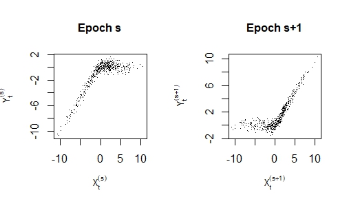
To show the advantage of assessing dependence through a copula function instead of via standard linear correlation-based methods, consider the following basic example. This example mimics the properties of rat local field potentials in this paper.For $t=1,...,500$, let $X_{t}^{(r)}$ and $Y_{t}^{(r)}$ be two random variables following the same dependence path for epochs $r=1,...,s$ such that $X_{t}\sim AR(1)$ of parameter $\phi=0.9$ and $Y_{t}^{(r)}=\mathcal{D}(X_{t}^{(r)})X_{t}^{(r)}+\epsilon_{t}^{(r)}$ where $\epsilon^{(r)}_{t}$ is a zero mean unit variance noise and $\mathcal{D}(X_{t}^{(r)})$ is the logistic curve $\exp\{-X_{t}^{(r)}\}/(1+\exp\{-X_{t}^{(r)}\})$. For epochs $r=s+1,...,R$, $X_{t}^{(r)}$ keeps following the same autoregressive process, but $Y_{t}^{(r)}=\mathcal{D}^{\prime}(X_{t}^{(r)})X_{t}^{(r)}+\epsilon_{t}^{(r)}$ where $\mathcal{D}^{\prime}(X_{t}^{(r)})=\exp\{X_{t}^{(r)}\}/(1+\exp\{X_{t}^{(r)}\})$. Thus, a changepoint in the dependence structure is present between epochs $s$ and $s+1$. Under this setup, a correlation-based changepoint detection method will not detect the change because the correlation between $X_{t}^{r}$ and $Y_{t}^{r}$ at epoch $r=s$ is not different from the correlation at epoch $r=s+1$. Theoretically, Pearson’s correlation will stay equal to approximately $0.80$. On Figure 2, one observes that, for epochs $r=1,...,s$, dependence is high in the lower tail and small in the upper tail; and for epochs $r=s+1,...,R$, one observes exactly the converse. However, the copula function catches these changes in the dependence structure. Indeed, under a right specification, two different copula models will be fitted: one for epochs $r=1,...,s$ and a completely different one for epochs $r=s+1,...,R$. Thus, with an adequate methodology to assess the equivalence between two copulas as discussed in this paper, a copula-based method will detect the changepoint between epochs $s$ and $s+1$, for which a correlation-based method fails.

We present in this article a copula-based framework to analyze changes between brain signals on given frequency bands for three different contexts. Firstly, we are interested in the detection of one (or many) changepoint(s) in the regime of a brain channel for a given frequency band. Secondly, we compare, within a single channel (microelectrode), if there is a difference in the dependence between successive epochs across the pre-stroke and post-stroke epochs. Thirdly, we compare the dependence structure of two different microelectrodes still on a given frequency band, on the entire recording time of $5$ minutes priot to and $5$ minutes post to the induced stroke.

The remainder of this paper is organized as follows. In Section 2, we present present briefly the transformation of time data to spectral data as well as the copula function in order to introduce our notation. In Section 3, we present the necessary theoretical background to introduce our models and algorithms. Then, in Sections 4, 5 and 6, we present analyses of the local field potential data recording during a span of $10$ minutes ($5$ minutes pre-stroke and $5$ minutes post-stroke). Our methodology directly applied to these data shows its performance by, at first, assessing the statistically significant changepoints in dependence between successive epochs for some specific channels. Secondly, it shows that the whole dependence structure between pre-stroke epochs is not significantly different, for all the channels, than the one for post-stroke epochs.

To facilitate ease of reading of the paper, we include the notations in Appendix A. Let ${\bf{X}}=\left[X_{1},X_{2},...,X_{d}\right]$ a three-dimensional matrix of dimension $T\times d\times R$ ($d$ brain channels divided into $R$ possibly over-lapping epochs (i.e., equal segmentation of $1$ second into $T$ time points)). Thus, one represents a single element of that matrix by $X_{\ell}^{(r)}(t)$, $\ell=1,...,d$; $t=1,...,T$; $r=1,...,R$, which might be seen as any recorded measure on channel $\ell$ during epoch $r$. Therefore, the 3-dimensional matrix is composed of $R$ matrices of size $T\times d$ denoted by ${\bf X}^{(r)}=[X_{1}^{(r)},\ldots,X_{d}^{(r)}]$.

This paper focuses on dependence among brain channels in the frequency domain. We remark that from the experimental perspective, the channels are defined by microelectrodes different parts of the brain. The Fourier coefficient for the channel $\ell=1,...,d$, at epoch $r=1,...,R$ and at fundamental Fourier frequency $\omega_{k}=k/T$ is defined to be

Because this transformation outputs single frequencies and in our context we are interested in frequency bands, we have to segregate frequencies according to the bands’ ranges and to smooth their magnitudes by averaging.

In this paper, we will study the dependence of magnitudes of the Fourier coefficients (or square roots of periodograms) between the different pairs of channels $\ell$ and $\ell^{\prime}$; $\ell,\ell^{\prime}=1,...,d$ for the same epoch $r$. In addition, we will investigate the dependence between successive pairs of epochs $r$ and $r+1$. We denote the frequency bands by $\Omega_{\kappa}$ where $\kappa=1,...,Q$ represents the frequency band, and where $Q$ is the number of frequency bands considered in this paper (see Section 3 for details about the chosen bands). Thus, $\Omega_{\kappa}$ is a collection of fundamental Fourier frequencies $\omega_{j}$, $j=\text{index}(\Omega_{\kappa}^{(\text{min})}),...,\text{index}(\Omega_{\kappa}^{(\text{max})})$ where $\text{index}(\Omega_{\kappa}^{(\text{min})})$ is the index of the first value constituting the frequency band among the $k$ fundamental frequencies, and $\text{index}(\Omega_{\kappa}^{(\text{max})})$ is the one of the last frequency constituting that band.

We now define ${\bf{\delta}}^{(r)}_{\Omega_{\kappa}}=[\delta_{1,\Omega_{\kappa}}^{(r)},...,\delta_{d,\Omega_{\kappa}}^{(r)}]$ which is the matrix of dimension $\text{card}(\Omega_{\kappa})\times d$ where any column is a different channel $\ell=1,...,d$. Therefore, each column is represented by $\delta_{\ell,\Omega_{\kappa}}^{(r)}=[|f_{\ell,\Omega_{\kappa}^{(\text{(min)})}}^{(r)}|,...,|f_{d,\Omega_{\kappa}^{(\text{(max)})}}^{(r)}|]^{\prime}$, a vector of length $\text{card}(\Omega_{\kappa})$ containing the magnitude for each Fourier fundamental frequency constituting the frequency band $\Omega_{\kappa}$ at epoch $r$. Hence, in the rest of this paper, we will consider $\delta_{\ell,\Omega_{\kappa}}^{(r)},\delta_{\ell^{\prime},\Omega_{\kappa}}^{(r)}$ as the random vectors on which our methodology is applied.

Prior to any statistical modeling, we applied a Fourier transform to the multichannel multiple-epoch brain signals, considering each microelectrode $\ell$ at each epoch $r$ as a single data vector. This transform was in order to obtain the values of the periodograms and then compute the magnitudes of these Fourier coefficients. As mentioned earlier, we decided to use frequency bands rather than single frequencies. To determine the range of the considered bands, we based our choice on a classical text in the literature: Buzsaki [6] about the rhythms of the brain. Hence, we adopted the following bands: $\Delta\in(0,4)$Hertz, $\theta\in(4,8)$Hertz, $\alpha\in(8,12)$Hertz, $\beta\in(12,30)$Hertz and $\gamma\geq 30$ Hertz. We note that in our applications, we truncated $\gamma$ at $300$ Hertz and applied a notch filter to remove the $60$ Hertz activity.

Before describing the specific cases where we assess the dependence among brain channels for particular frequency bands, we first discuss the application of the Kolmogorov-Smirnov statistic to the multivariate setting. Kolmogorov-Smirnov might be used to compare two cdf together. In the univariate case, if $A(x)$ and $B(x)$ are two cdf, to test $H_{0}:A=B$ versus $H_{1}:A\neq B$, we use the statistic

which is known to converge almost surely to 0 under $H_{0}$ due to Donsker’s theorem[13].

In this paper, we are interested in the empirical value of that statistic in a multivariate context. We use it in different ways according what we study. However, the way that we deal with the statistics of test remains the same. In a bivariate situation, let ${\bf{X}}=(X_{1},X_{2})^{\prime}$ and ${\bf{Y}}=(Y_{1},Y_{2})^{\prime}$ be two random variables with respective joint cdf $A$ and $B$. Also, let $u,v$ be two finite partitions in any closed subset of $\mathbb{R}^{2}$, large enough to contain the supports of $\bf{X}$ and $\bf{Y}$. Hence, we define our computational approach of the bivariate Kolmogorov-Smirnov statistic as

where $C_{\bf{X}},C_{\bf{Y}}$ are respectively the unique copulas equal to $A$ and $B$ according to Sklar. In practice, variables are on different supports (e.g., the amplitude of signals for $\delta$-frequency band versus the one for $\beta$-frequency band) and finding a finite grid of values $u$ and $v$ containing the support of both $\bf{X}$ and $\bf{Y}$ might be a tricky task. That is the reason why we standardize data into the $[0,1]$ interval (see how in Section 4).

Under a real equality in distribution for $C_{\bf{X}}$ and $C_{\bf{Y}}$, for $\tilde{u}\in[0,1]$ and $\tilde{v}\in[0,1]$ standardized versions of $u$ and $v$ being vectors of sufficiently large dimension, the statistic $D_{\bf{\tilde{X},\tilde{Y}}}$, where ${\bf{\tilde{X},\tilde{Y}}}$ are standardized versions of $\bf{X},\bf{Y}$, is nothing more than the bivariate version of the usual Kolmogorov-Smirnov statistic.

A remaining issue with Kolmogorov-Smirnov is that the validity of this statistic relies on the robustness of the distributions. However, due to the cardinality of the low-frequencies bands, estimating any parameter directly on these bands will lead to non-robust distributions. That is the reason why one has to use resampling techniques in order to obtain some distributions and then derive their parameters (e.g., mean and standard deviation).

To illustrate the pertinence of the dependence issues related to brain signals for certain frequency bands, here we use experimental data from Wann [39] on local field potentials measured on rats’ cortex. To summarize that experiment, local field potentials were recorded from $32$ microelectrodes placed on $4$ cortical layers (each with $8$ electrodes). This setup is illustrated in Figure 3. On these $32$ microelectrodes (channels), using insulated stainless steel wire electrodes, data have been recorded for 5 minutes where each second represents a single epoch which consists of $T=1000$ time points. After these five minutes, a stroke have been mechanically induced using an hemostat clamp on the brain artery located on the second column of electrodes (from the left) recording microelectrodes $2,10,18$ and $26$. Then, for five minutes, data, divided in the same way as the previous five minutes, has been recorded.

Our interest in this section is to identify the epoch $r^{*}$ where the dependence between successive epochs $r^{*}-1$ and $r^{*}$ differ from the dependence between epochs $r^{*}$ and $r^{*}+1$. Hence, we are interested to identity that epoch $r^{*}$ for each microelectrode for all the $\Omega_{\kappa}\in\{\Delta,\theta,\alpha,\beta,\gamma\}$ frequency bands. With LFP data, the dependence between $\delta_{\ell,\Omega_{\kappa}}^{(r)}$ and $\delta_{\ell,\Omega_{\kappa}}^{(r+1)}$ (no matters if these epochs are considered as a changepoint or not) exhibit frequently complex structure. For example, on Figure 5, one sees (for rat id $141020$) for microelectrode (channel) $17$ some structures where the magnitudes of the Fourier coefficients for two successive epochs are highly dependent in their lower tail, and become more and more independent as they one moves toward their higher tail. This particular structure is easily representable through a copula function (Clayton copula will be considered in this case), but is not through any linear correlation (specifically coherence in the spectral domain) structure. For channel $1$ (Figure 4) , one notices, still for the same rat, that the dependence structure change with stroke: for example, one notices the difference between the upper tails. This difference gets more and more obvious as we are looking for dependence between these magnitudes for epochs which get closer to the temporal interval: epochs $375$ to $380$. One notices that data in the first row are the one used in our algorithm. However, for a visualization purpose, data are log scaled in the second row in order to respond to skewness of large magnitude values.

For this data, the expected major changepoint is $r^{*}=301$ which is the stroke onset. It is likely too that other changepoints would be observed after the stroke. However, for some biological issues, the peak of this observation might be delayed between the $375$$-th$ and the $380$$-th$ epoch (from $75$ to $80$ seconds after the stroke) for a majority of the frequency channels, on most of their frequency bands. We observe that this $5-$seconds activity window is subject to change in function of the rat on which experiment is conducted. We note that the way we segregated epochs (changepoint vs stable epoch) is based on the empirical setting presented in 4.1.

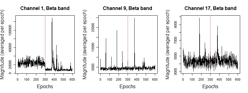
We remark that, without regard to the frequency band, mainly three patterns are present in the regime of $\delta_{\ell,\Omega_{\kappa}}^{(1:600)}=[\delta_{\ell,\Omega_{\kappa}}^{(1)},...,\delta_{\ell,\Omega_{\kappa}}^{(600)}]$ with rat id $141020$. An interesting fact is that even if the location of the clamped artery is on column $2$, these three patterns are observed on column $1$. They are respectively microelectrodes (channels) $1$, $9$ and $17$. Figure 6 exhibits the averaged amplitude (per epoch) for each one of these microelectrodes. The results for these three microelectrodes (for the five frequency bands) are presented as these are representative of our methodology.

Algorithm 1 presents the proposed methodology to detect one or many changepoint(s) in the regime of a channel for a given frequency band. Some remarks are as follows. Firstly, in this algorithm, we adopt the tilde notation (e.g., $\tilde{\delta}_{\ell,\Omega_{\kappa}}^{(r)}$) to differentiate standardized variables from regular variables, but in this paper we assume all variables to be standardized after this step. Therefore, we will no longer use this notation in order to simplify the text. Also, still in the same step, note that we use unique minimum and maximum over all the $600$ epochs range. It is crucial to use these standardization values in order to get comparable Kolmogorov-Smirnov statistics. Secondly, our panel of copulas consists only of Archimedean models in order to avoid potential problems of comparing widely different models. Finally, the thresholds for the Kolmogorov-Smornov statistics are determined empirically and the procedure is described in Section 4.1.

Our goal here is to compare the spectral dependence of the magnitude of Fourier coefficients pre-stroke versus the one post-stroke (i.e., to compare for a fixed microelectrode - understand ”a fixed channel”- and a fixed frequency band if there is a change in the entire structure of dependence among the $300$ epochs before the stroke versus after).

To do so, consider a given frequency band $\Omega_{\kappa}$, $\kappa=1,...,Q$. We define the multivariate matrices $\delta_{\ell,\Omega_{\kappa}}^{(1:300)}=[\delta_{\ell,\Omega_{\kappa}}^{(1)},...,\delta_{\ell,\Omega_{\kappa}}^{(300)}]$ and $\delta_{\ell,\Omega_{\kappa}}^{(301:600)}=[\delta_{\ell,\Omega_{\kappa}}^{(301)},...,\delta_{\ell,\Omega_{\kappa}}^{(600)}]$ (two matrices of dimension $\text{card}(\Omega_{\kappa})\times 300$) as two single structures of the dependence. Using straightforwardly a single parametric copula in each case would be an enormous mistake. In fact, the parameter(s) of any Archimedean copula is too general to represent at the same time both the dependence measure between $\delta_{\ell,\Omega_{\kappa}}^{(1)}$ and $\delta_{\ell,\Omega_{\kappa}}^{(2)}$ and the dependence measure between $\delta_{\ell,\Omega_{\kappa}}^{(r)}$ and $\delta_{\ell,\Omega_{\kappa}}^{(r+1)};r=2,...,299$. That’s the reason why we propose here to use vine copulas (for information, see see Bedford and Cooke [4] and Aas et al. [1]) to represent the dependence between these sets of variables.

The principle of vine copulas is the representation of a multivariate copula as a nested network of bivariate copulas where each single copula is named a node and each link between two nodes (defining the order of the copulas and their relations among themselves) is named an edge. Each level of dependence in this nested network is named a tree. For all type of vines, the first tree is always the set of copulas between the univariate nodes (variables) and for the following trees, the nodes are always conditionals to at least one variable.

In this paper, due to the temporal relation between the consecutive $\delta_{\ell,\Omega_{\kappa}}^{(r)},r=1,...,600$, we assume the structures of dependence for the multivariate sets $\delta_{\ell,\Omega_{\kappa}}^{(1:300)}$ and $\delta_{\ell,\Omega_{\kappa}}^{(301:600)}$ being represented by drawable vine (D-Vine) copulas. In other words, we assume that the edge between any node in the first tree only link the consecutive variables $\delta_{\ell,\Omega_{\kappa}}^{(r)},\delta_{\ell,\Omega_{\kappa}}^{(r+1)};r=1,...,599$.

Obviously, we cannot use a 300-variate version of the Kolmogorov-Smirnov statistic to compare $\delta_{\ell,\Omega_{\kappa}}^{(1:300)}$ to $\delta_{\ell,\Omega_{\kappa}}^{(301:600)}$. It is still computationally unfeasible. That’s the reason why, in our work, we propose to adapt a test comparing two vine copulas models (see Clarke [8])to our context consisting in determining any difference in the structure of dependence between them. We remark that this test is mainly used in the literature in a goodness of fit perspective of a vine structure given a set of data. Since $\delta_{\ell,\Omega_{\kappa}}^{(1:300)}$ and $\delta_{\ell,\Omega_{\kappa}}^{(301:600)}$ are two different set of data having the same dimensionality which does not need to be independent, it is appropriate to use it.

The principle of that test is as follow. Let the ratios of the log-likelihhood for each Fourier frequency in the band under consideration $m_{i;\ell,\Omega_{\kappa}}=\text{log }\left\{\frac{c^{(1:300)}_{\ell,\Omega_{\kappa}}({\bf{u}}_{i}|\theta^{(1:300)}_{\ell,\Omega_{\kappa}})}{c^{(301:600)}_{\ell,\Omega_{\kappa}}({\bf{u}}_{i}|\theta^{(301:600)}_{\ell,\Omega_{\kappa}})}\right\}$, $i=1,...,\text{card}(\Omega_{\kappa})$ where $c$ stands for the density of a D-Vine copula function, $\theta^{(1:300)}_{\ell,\Omega_{\kappa}},\theta^{(301:600)}_{\ell,\Omega_{\kappa}}$ the vectors of the copula parameters for each vine structure and ${\bf{u}}_{i}$ the vector of observations. Thus, if there is no difference between the vine copulas of the sets of variables $\delta_{\ell,\Omega_{\kappa}}^{(1:300)}$ and $\delta_{\ell,\Omega_{\kappa}}^{(301:600)}$, the ratios of the log-likelihhood $m_{i;\ell,\Omega_{\kappa}}$ should be uniformly distributed around zero and $50\%$ of them should be greater than 0 (for details and proof, see Vuong [38]). Thus, we are testing for all $i=1,...,\text{card}(\Omega_{\kappa})$:

Therefore, the statistic of test is

where $\mathds{1}$ stands for the indicator function. Then, under the null hypothesis, $\xi_{\ell,\Omega_{\kappa}}\sim\mathcal{B}\text{{in}}(\text{card}(\Omega_{\kappa}),0.5)$ and we can interpreted the statistic of test such that the vine copula pre-stroke is statistically equivalent to the one post stroke if $\xi$ is not statistically different from $\mathbb{P}(m_{i;\ell,\Omega_{\kappa}}\leq 0)\times\text{card}(\Omega_{\kappa})=0.5\text{card}(\Omega_{\kappa})$ for a given significance level. This test is known as Clarke’s test [8] and has been considered in most of the literature comparing two vine structures (see Joe and Kurowicka [23]).

We performed our version of that test on the gamma band for the whole LFP data set, as it is the one where we can visually observe on some channels aspects of change and on some other channels aspect of stability. We note that, in order to reduce noise, we truncated gamma band to $300$ $Hz$ such that $\gamma\in\{30,300\}Hz$. Figure 9 shows, for rat id $141020$, in the way the electrodes are placed in the rat’s brain the p-value obtained for each channel. In Appendix C, one observes the statistics of test we obtained for each channel (second row) as well as these p-values for each one of the four rats. Microelectrodes in black suggest to accept $H_{0}$ for a significance level of $2.5\%$. Thus, under that significance level, we can say that for $\gamma$-band, there are no strong evidences of a change in the brain activity of the rat after the induced stroke for channels $1,2,13,14,15,16\text{ and }23$.

This section is in fact a brief note to show that one can apply the methodology from Section 5 to compare, based on the dependence structure, if two different microelectrodes (brain channels), for a given frequency band, act similarly during all the regime of the experiment (i.e., during the $600$ epochs). Thus, we test exactly the same hypothesis but this time, $m_{i;\ell,\ell^{\prime};\Omega_{\kappa}}$ is defined differently. For epochs $1$ to $600$, this log-likelihood ratio is defined by:

where $i=1,...,\text{card}(\Omega_{\kappa})$, and $\ell$ and $\ell^{\prime}$ are obviously two different channels. We applied this test to the channels defined on the two first columns of microelectrodes in the rat brain (i.e., channels linked to microelectrodes $1,2,9,10,17,18,25$ and $26$; which means a total of $28$ possible combinations). We show the results for the gamma band, for the four experimental rats, in Appendix C (Table 4). We remind that to not reject $H_{0}$, the Clarke’s statistic of test must not be significantly different to $\text{card}(\Omega_{\kappa})/2$. As the results are for gamma band, they should not be significantly different to $(300\text{Hz}-31{Hz})/2=135$ under $H_{0}$. That said, even if the Clarke’s statistics are valued on a wide range from $0$ to $270$, one observes that these $8$ channels are considered being completely different on their whole regime for a significance level: the p-values are always lower than $0.0001$ for all the $28$ possible combinations.

This paper related some approaches to assess both the dependence and the information we can learn from that dependence (i.e. changepoint, change in a regime, etc.). By considering more complex structures than simply linear relations (e.g., linear correlation, coherence) to assess dependence between brain signals, we modeled the relations between these signals. We also proposed algorithms with which we determined if one can presume a change or not on these complex structures of dependence. Such a methodology aims to show his utility in the future because research about specific types of strokes like CVA gets more and more funded in order to do prevention in the society.

In closing, we address two potential criticisms of the proposed work. Firstly, we used only parametric copula models when it is true that in general, non-parametric models are more flexible to data. But in our context, the dimension of some frequency bands is not large enough to ensure the robustness of a nonparametric model as a parametric model might be. Secondly, the analysis was conducted only on four rats. It is true that data from many more rats will increase the power of the neurological conclusions. However, the work done here was an explanatory study of a copula-based approach for such data, and having to analyze data from many more rats will complexity the computational work. Many future research avenues are possible from what we did. One of these avenues is to study the impact of taking copulas on more than $2$ epochs while processing the iterative algorithm when studying a changepoint for a single brain channel. Indeed, it will allow to detect changes that occur for small windows of time instead that punctually. Another one is to study our copula-based approach the possible lagged dependence(s) between two different frequency bands.

Ron D. Frostig was supported by the Leducq Foundation (grand 15CVD02).

References

- [1] Aas, K., C. Czado, A. Frigessi, and H. Bakken (2009). Pair-copula constructions of multiple dependence. Insurance: Mathematics and economics 44(2), 182–198.
- [2] Adak, S. (1998). Time-dependent spectral analysis of nonstationary time series. Journal of the American Statistical Association 93(444), 1488–1501.
- [3] Akaike, H. (1998). Information theory and an extension of the maximum likelihood principle. In Selected Papers of Hirotugu Akaike, pp. 199–213. Springer.
- [4] Bedford, T. and R. M. Cooke (2002). Vines: A new graphical model for dependent random variables. Annals of Statistics, 1031–1068.
- [5] Brockwell, P. J. and R. A. Davis (2013). Time series: theory and methods. Springer Science & Business Media.
- [6] Buzsaki, G. (2006). Rhythms of the Brain. Oxford University Press.
- [7] Cech, C. (2006). Copula-based top-down approaches in financial risk aggregation.
- [8] Clarke, K. A. (2007). A simple distribution-free test for nonnested model selection. Political Analysis 15(3), 347–363.
- [9] Dauwels, J., H. Yu, X. Wang, F. Vialatte, C. Latchoumane, J. Jeong, and A. Cichocki (2012). Inferring brain networks through graphical models with hidden variables. In Machine Learning and Interpretation in Neuroimaging, pp. 194–201. Springer.
- [10] Davis, R. A., T. C. M. Lee, and G. A. Rodriguez-Yam (2006). Structural break estimation for nonstationary time series models. Journal of the American Statistical Association 101(473), 223–239.
- [11] Dette, H. and T. Hildebrandt (2012). A note on testing hypotheses for stationary processes in the frequency domain. Journal of Multivariate Analysis 104(1), 101–114.
- [12] Dette, H. and E. Paparoditis (2009). Bootstrapping frequency domain tests in multivariate time series with an application to comparing spectral densities. Journal of the Royal Statistical Society: Series B (Statistical Methodology) 71(4), 831–857.
- [13] Donsker, M. D. (1952). Justification and extension of doob’s heuristic approach to the kolmogorov-smirnov theorems. The Annals of mathematical statistics, 277–281.
- [14] Efron, B. and R. J. Tibshirani (1994). An introduction to the bootstrap. CRC press.
- [15] Fiecas, M. and H. Ombao (2016). Modeling the evolution of dynamic brain processes during an associative learning experiment. Journal of the American Statistical Association 111(516), 1440–1453.
- [16] Fontaine, C. and H. Ombao (2018). Dependence between time series using spectral-based measures within copula inference.
- [17] Genest, C. and R. J. MacKay (1986). Copules archimédiennes et families de lois bidimensionnelles dont les marges sont données. Canadian Journal of Statistics 14(2), 145–159.
- [18] Gotman, J. (1982). Automatic recognition of epileptic seizures in the eeg. Electroencephalography and clinical Neurophysiology 54(5), 530–540.
- [19] Grønneberg, S. and N. L. Hjort (2014). The copula information criteria. Scandinavian Journal of Statistics 41(2), 436–459.
- [20] Ince, R. A., B. L. Giordano, C. Kayser, G. A. Rousselet, J. Gross, and P. G. Schyns (2017). A statistical framework for neuroimaging data analysis based on mutual information estimated via a gaussian copula. Human brain mapping 38(3), 1541–1573.
- [21] Iyengar, S. G., J. Dauwels, P. K. Varshney, and A. Cichocki (2010). Quantifying eeg synchrony using copulas. In Acoustics Speech and Signal Processing (ICASSP), 2010 IEEE International Conference on, pp. 505–508. IEEE.
- [22] James, N. A. and D. S. Matteson (2015). Change points via probabilistically pruned objectives. arXiv preprint arXiv:1505.04302.
- [23] Joe, H. and D. Kurowicka (2011). Dependence modeling: vine copula handbook. World Scientific.
- [24] Jordanger, L. A. and D. Tjøstheim (2014). Model selection of copulas: Aic versus a cross validation copula information criterion. Statistics & Probability Letters 92, 249–255.
- [25] Kifer, D., S. Ben-David, and J. Gehrke (2004). Detecting change in data streams. In Proceedings of the Thirtieth international conference on Very large data bases-Volume 30, pp. 180–191. VLDB Endowment.
- [26] Lavielle, M. (1999). Detection of multiple changes in a sequence of dependent variables. Stochastic Processes and their Applications 83(1), 79–102.
- [27] Lavielle, M., C. Ludeña, et al. (2000). The multiple change-points problem for the spectral distribution. Bernoulli 6(5), 845–869.
- [28] Long, C., E. N. Brown, D. Manoach, and V. Solo (2004). Spatiotemporal wavelet analysis for functional mri. NeuroImage 23(2), 500–516.
- [29] Nelsen, R. B. (2007). An introduction to copulas. Springer Science & Business Media.
- [30] Nunez, P. L., R. Srinivasan, et al. (2006). Electric fields of the brain: the neurophysics of EEG. Oxford University Press, USA.
- [31] Ombao, H., M. Lindquist, W. Thompson, and J. Aston (2016). Handbook of Neuroimaging Data Analysis. Chapman and Hall/CRC.
- [32] Ombao, H. C., J. A. Raz, R. von Sachs, and B. A. Malow (2001). Automatic statistical analysis of bivariate nonstationary time series. Journal of the American Statistical Association 96(454), 543–560.
- [33] Politis, D. N. and J. P. Romano (1994). The stationary bootstrap. Journal of the American Statistical association 89(428), 1303–1313.
- [34] Purdon, P. L., V. Solo, R. M. Weisskoff, and E. N. Brown (2001). Locally regularized spatiotemporal modeling and model comparison for functional mri. NeuroImage 14(4), 912–923.
- [35] Radovanov, B. and A. Marcikić (2014). A comparison of four different block bootstrap methods. Croatian Operational Research Review 5(2), 189–202.
- [36] Schwarz, G. et al. (1978). Estimating the dimension of a model. The annals of statistics 6(2), 461–464.
- [37] Sklar, M. (1959). Fonctions de repartition an dimensions et leurs marges. Publ. inst. statist. univ. Paris 8, 229–231.
- [38] Vuong, Q. H. (1989). Likelihood ratio tests for model selection and non-nested hypotheses. Econometrica: Journal of the Econometric Society, 307–333.
- [39] Wann, E. G. (2017). Large-scale spatiotemporal neuronal activity dynamics predict cortical viability in a rodent model of ischemic stroke. Ph. D. thesis, UC Irvine.
- [40] White, H. (1982). Maximum likelihood estimation of misspecified models. Econometrica: Journal of the Econometric Society, 1–25.
Appendix A Table of notation