The Combinatorial Data Fusion Problem
in Conflicted-supervised Learning

Categorical machine learning tasks may be cast as vertex labelling problems on large, edge-weighted graphs. Examples include (1) mapping the pixels of an image to parts of an object depicted in the image, (2) mapping web sites to functional categories of web services, (3) discriminating between fraudulent and authentic credit card transactions, (4) allocating mobile handsets to specific communication channels. Suppose $V_{o}$ denotes the objects to be labelled, and $V_{c}$ the set of labels. Information available to us is of three kinds:

1. 1.

   Partial labelling: Some objects in $V_{o}$ already carry labels. Express this by an edge $\{v,\phi(v)\}$ between $v\in V_{o}$ and its label $\phi(v)\in V_{c}$, weighted to reflect strength of association.

2. 2.

   Label equality: For some pairs $u,v\in V_{o}$, a weighted edge $\{u,v\}$ expresses evidence that $u$ and $v$ should carry the same (as yet undeclared) label.

3. 3.

   Prohibitions: There are some subsets of $V_{o}$ called forbidden sets. Not all vertices in a forbidden set may be assigned the same label. In data base contexts, for example, such prohibitions occur when there is evidence that two objects with similar or identical names are actually distinct.

The three kinds of information mentioned above typically come from disparate sources, and may partially contradict each other. In Table 1, we call this conflicted-supervised learning. The data scientist is asked to perform a best merge of these data sources to arrive at a vertex labelling.

In a semi-supervised learning graph problem, by contrast, few vertices have been labelled, and the task is to extend this labelling to all vertices in a way that respects the adjacency structure, as in [17]. Such label propagation in graphs can be achieved through random walks, belief propagation, semi-definite programming, etc.; see references in Darling & Velednitsky [7].

Combinatorial data fusion, as introduced here, is a rigorous approach to conflicted-supervised learning. By deleting graph edges, break the graph into components, each of which contains at most one of the label vertices in $V_{c}$. If $v\in V_{o}$ is in a component with a unique $V_{c}$ vertex then $v$ receives that as its label. For a component without a $V_{c}$ vertex a new distinct label is created and all vertices within that component receive the new label. Note that the label received by a vertex may not agree with the vertex’s original label, and some label vertices may end up isolated. The aim is to minimize the total weight of deleted edges of types 1. and 2., so to enforce all the prohibitions in 3. Instead of label propagation, existence of forbidden sets leads to label dissociation. The approach taken here builds on the machinery of graph cuts.

For the sake of concreteness, here is an over-simplified example, which we abstract in Section 8.1.1. You are the manager of an online market place in which various vendors offer products for sale, whose union is a set $V_{o}$. Vendors are expected to label each item in $V_{o}$ with one of a set $V_{c}$ of exclusive categories, but some vendors fail to do so, or label incorrectly, perhaps because the categories are difficult to understand. Set $V:=V_{o}\cup V_{c}$ as a vertex set, with two types of weighted edges:

1. 1.

   If vendor $k$ assigns product $v\in V_{o}$ to category $c:=\phi_{k}(v)\in V_{c}$, place weight $w_{k}>0$ on edge $\{v,c\}$. Less reliable vendors receive less weight.

2. 2.

   If transaction data indicate that $m$ buyers have bought both $v,v^{\prime}\in V_{o}$, assign weight $w_{m}^{\prime}>0$ to edge $\{v,v^{\prime}\}$, where $m\mapsto w_{m}^{\prime}$ is increasing. The idea is that common buyers suggest two items belong to the same category.

In exclusive categorization, the forbidden sets are $\{\{c,c^{\prime}\},c\neq c^{\prime}\in V_{c}\}$, and combinatorial data fusion becomes a multiway cut problem, discussed in Section 2.5. When categories are difficult to understand, a forbidden set might take the form $\{c,c^{\prime},c^{\prime\prime}\}$, meaning that the three categories are not identical, but possibly two out of three may coincide. In summary, the goal is best merge of vendor labelling data with sales transaction data. The output of the algorithm will be an assignment of each product to a category, possibly different to the one assigned by the vendor.

The present work covers fundamental definitions and functorial properties, and solution methods when the underlying graph is a tree, or is approximated by a tree. Future works will cover linear programming relaxations, and cases where forbidden sets are not given explicitly, but are returned by an oracle which decides whether a system of linear inequalities has a feasible point.

Given a set $V$, and a collection $\mathcal{S}$ of subsets of $V$, we call $(V,\mathcal{S})$ an independence system if $U\in\mathcal{S}$ and $W\subset U$ implies $W\in\mathcal{S}$, and $\emptyset\in S$. Elements of $\mathcal{S}$ are called independent sets. A subset $W\subset V$ which is not in $\mathcal{S}$ is called a dependent set. Minimal dependent sets are called circuits. The collection of circuits of an independence system $(V,\mathcal{S})$ is denoted $\mathbf{C}(\mathcal{S})$. The next assertion is part of Korte and Vygen [8, Theorem 13.12].

In practical applications, the most parsimonious specification of an independence system may be its set of circuits. Circuits are discussed further in Schrijver [11, vol. B, Section 39.6].

Let $V$ be a finite vertex set on which two separate combinatorial structures are defined:

1. 1.

   An edge-weighted graph $G=(V,E_{0},w)$, with weights $w:E_{0}\rightarrow(0,\infty)$. With no loss of generality, assume $G$ is connected¹¹ 1 If $G$ is not connected, then each graph component may be treated as a separate problem..

2. 2.

   An independence system $\mathcal{S}$, which includes all singletons²² 2 This implies every forbidden set has cardinality at least two. and all edges in $E_{0}$ (i.e. $\{\{v\}|v\in V\}\cup E_{0}\subset S$). The circuits $\mathbf{C}(\mathcal{S})=:\mathcal{F}$ are called forbidden sets. Call $H:=(V,\mathcal{F})$ the forbidden hypergraph, and call $A:=(V,\mathcal{S})$ the allowable hypergraph.

What we call data fusion occurs between the forbidden hypergraph $H=(V,\mathcal{F})$, and the weighted graph $G=(V,E_{0},w)$. More specifically, the data fusion problem is looking for an optimal, with respect to $w$, subgraph of $G$ which avoids all the structures that the forbidden hypergraph disallows. To make this precise, three combinatorial formulations of the same problem are given below.

The combinatorial data fusion problem $(V,E_{0},w,\mathcal{F})$ refers to any of the three optimization problems above. Indeed:

Remark: An optimum may be called an optimum hypergraph coloring in the context (2), a maximum subgraph in the context (1), or a maximum hypergraph matching in the context (4).

Let $G=(V,E_{0},w)$ be a weighted graph and let $S_{1},S_{2},\dots,S_{k}$ be $k$ sets of vertices. Avidor & Langberg [1] define the multi-multiway cut problem (MMC) as finding a subset $E_{2}\subset E_{0}$ of minimum total weight such that the $S_{i}$ are completely disconnected in $(V,E_{0}\setminus E_{2})$ (i.e. if $u,v\in S_{i}$ for some $i$ then $u$ and $v$ are disconnected in $(V,E_{0}\setminus E_{2})$ ). The multiway cut problem is the sub-case where $k=1$, meaning that there is only one set of vertices that have to be pairwise disconnected; see Chapter 8 of Williamson & Shmoys [14] and Chapters 4 and 19 of Vazirani [15]. Dahlhaus et al [6] proved this problem to be NP-Hard. Recently Velednitsky & Hochbaum [16] showed that an algorithm which gives a 2-approximation actually gives an optimum when the graph is 2-stable. The more familiar multicut problem, discussed in section 2.6, is the sub-case where $|S_{i}|=2$ for $1\leq i\leq k$. This is NP-hard except when $k=2$, and is analyzed at length by Williamson & Shmoys [14] and Vazirani [15].

Contrast the multi-multiway cut problem with the combinatorial data fusion problem on the same $G$ where $S_{1},S_{2},\dots,S_{k}$ are the forbidden sets. For the latter, removal of edges needs only to ensure that the $S_{i}$ are not connected, whereas in the former each $S_{i}$ must be completely disconnected. The multi-multiway cut problem is a special case of the combinatorial data fusion problem where the forbidden sets are all pairs of vertices contained in the $S_{i}$ (i.e. $\mathcal{(}F)=\{(u,v)|u,v\in S_{i},1\leq i\leq k\}$).

The combinatorial data fusion problem extends multicut in that forbidden sets of cardinality larger than two are allowed. Here is an example showing the need for this greater generality.

Bishop and Darling [2] consider sporadic observation of a moving target. Take an observation set $\mathcal{O}$, which consists of a collection of pairs

where $0\leq t_{1}<t_{2}<\cdots<t_{n}\leq T$ are the observation times, and each $K_{i}$ is a convex polygon ${\mathbf{R}}^{d}$ under the Manhattan metric. In that case, membership in $K_{i}$ can be checked using a finite system of linear inequalities, as can the non-emptiness of the set

where $B$ is a positive speed bound. To say that $\Lambda_{B}(\mathcal{O})$ is empty is equivalent to saying that a traveler with maximum speed $B$ could not have visited zone $K_{i}$ at time $t_{i}$ for every $i$, in which case we call the observation set incompatible with $B$; otherwise it is compatible.

Evidently the collection of subsets $X\subset\mathcal{O}$ such that $X$ is compatible with $B$ is an independence system, and its circuits can be taken as the forbidden sets $\mathcal{F}$ in a combinatorial data fusion problem. The enumeration of such circuits is the problem addressed by Boros et al [3]. For example, a forbidden set of size three consists of three observations $(t_{1},K_{1}),(t_{2},K_{2}),(t_{3},K_{3})$ which are incompatible with $B$, while every subset of size two is compatible. See Figure 2 for a planar example under the Euclidean metric.

At least two types of combinatorial data fusion problem appear in this context.

Carlsson and Mémoli [4] propose that a clustering algorithm should be a functor from a suitable category of finite metric spaces into a suitable category of partitioned sets⁵⁵ 5 Carlsson and Mémoli call this the category of outputs of standard clustering schemes.. Their categorical definitions are designed to achieve the following algorithmic property. Suppose $\phi:X\to Y$ is an injective, non-expansive map between finite metric spaces. Such a map could arise, for example, when a data set $X$ is augmented by additional data points. Suppose points $x,x^{\prime}\in X$ are assigned to the same cluster when a specific clustering algorithm is applied to $X$; then $\phi(x),\phi(x^{\prime})\in Y$ should be in the same cluster when the same algorithm is applied to $Y$.

Use the term partitioned set to denote a pair $(X,\mathcal{P})$, where $X$ is a set, and $\mathcal{P}$ is a partition of $X$. View $\mathcal{P}$ as a collection of subsets $\{X_{\alpha}\}_{\alpha\in A}$ of $X$ which we call the blocks of the partition.

Define the category of partitioned sets as follows. Objects are partitioned sets $(X,\mathcal{P})$ with $X$ finite. The morphisms from $(X,\mathcal{P})$ to $(Y,\mathcal{Q})$ consist of set mappings $\phi:X\to Y$ with the property⁶⁶ 6 Equivalent to: $\mathcal{P}$ is a refinement of the pullback of $\mathcal{Q}$ under $\phi$. : if points $x,x^{\prime}\in X$ are in the same block of $\mathcal{P}$, then $\phi(x),\phi(x^{\prime})\in Y$ are in the same block of $\mathcal{Q}$.

Carlsson and Mémoli’s program inspired us to ask whether there exists some notion of morphism between a pair of combinatorial data fusion problems, such that data fusion algorithms are functors into the category of partitioned sets.

Suppose $(V,E)$ and $(V^{\prime},E^{\prime})$ are graphs, while $(V,\mathcal{S})$ and $(V^{\prime},\mathcal{S}^{\prime})$ are independence systems, also called abstract simplicial complexes.

Observe that the weight functions on $E$ and $E^{\prime}$ play no part in this definition.

Let $(V,E,w,\mathcal{F})$ and $(V^{\prime},E^{\prime},w^{\prime},\mathcal{F}^{\prime})$ be a pair of combinatorial data fusion problems, where $\mathcal{F}$ are the circuits of $\mathcal{S}$, and $\mathcal{F}^{\prime}$ are the circuits of $\mathcal{S}^{\prime}$. Let $\phi:V\to V^{\prime}$ be a weak morphism of these combinatorial data fusion problems.

Suppose a partition $V_{0},V_{1},\ldots,V_{d-1}$ of $V$ forms a maximum weight matching of $(V,\mathcal{S})$ under $w$, as in Section 2.3.3. Is it necessarily a refinement of $\phi^{-1}(V_{0}^{\prime}),\phi^{-1}(V_{1}^{\prime}),\ldots,\phi^{-1}(V_{f-1}^{\prime})$, for some maximum weight matching $V_{0}^{\prime},V_{1}^{\prime},\ldots,V_{f-1}^{\prime}$ of $(V^{\prime},\mathcal{S}^{\prime})$ under $w^{\prime}$, by analogy with Carlsson and Mémoli’s paradigm?

The counterexamples of Figures 3 and 4 show two important kinds of mis-match between two such combinatorial data fusion problems, linked by a weak morphism.

1. 1.

   Suppose $(V,E)$ is a vertex-induced subgraph of $(V^{\prime},E^{\prime})$, which means that $E$ is precisely the edges in $E^{\prime}$ with both endpoints in $V$. Suppose $\mathcal{F}^{\prime}=\mathcal{F}$, so the only forbidden sets in $V^{\prime}$ are the ones in $V$. Certainly the inclusion map $\iota:V\to V^{\prime}$ is a weak morphism. Figure 3 shows how, even with a single forbidden set $\{v_{1},v_{2},v_{3}\}$, the unique maximum weight matching of $(V,\mathcal{S})$ is not a refinement of the unique maximum weight matching of $(V^{\prime},\mathcal{S}^{\prime})$.

   

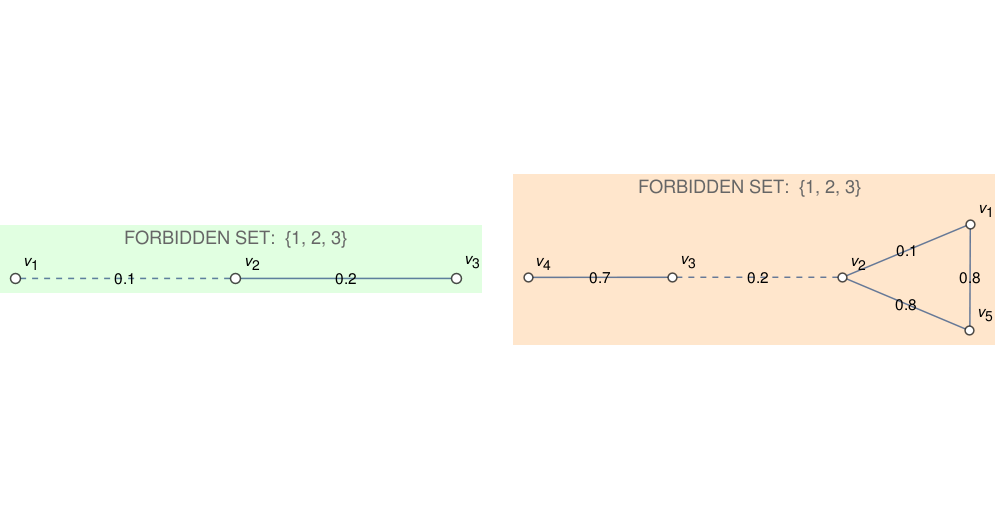
2. 2.

   Take the graphs $(V,E,w)$ and $(V^{\prime},E^{\prime},w^{\prime})$ as identical, but $\mathcal{S}\subsetneq\mathcal{S}^{\prime}$. From the forbidden sets perspective, $\mathcal{F}\supsetneq\mathcal{F}^{\prime}$ In Figure 4, $|\mathcal{F}|=2$ (right side), while $|\mathcal{F}^{\prime}|=1$ (left side). The unique maximum weight matching of $(V,\mathcal{S})$ is not a refinement of the unique maximum weight matching of $(V^{\prime},\mathcal{S}^{\prime})$.

   

Before studying algorithms, let us take a look at the space of optimum solutions. In this section we shall study the number of colors that are required in an optimal coloring.

The number of colors (or equivalently the number of connected components in a subgraph, or hyperedges in an optimal perfect matching) does not appear in the combinatorial data fusion objective function. However, monochromatic $G$ edges do appear in the objective function and the more colors used in a coloring of $H$ the harder it is to maintain monochromatic edges in $G$. Additionally, some algorithmic techniques put a limit on the number of allowable colors and/or have the number of colors appear in their run time.

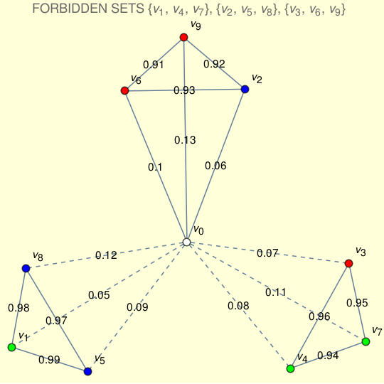
It is natural to wonder about the interaction between the forbidden sets of a combinatorial data fusion problem, and the color classes of an optimal solution. For example, when every forbidden set has size at least $k$, and the number of colors in an optimum hypergraph coloring does not exceed $k$, must each color necessarily have a representative vertex in each forbidden set? This is tautologically true if $k=2$, but false in general for $k\geq 3$.

Figure 5 offers a counterexample. Even when the forbidden sets are pairwise disjoint, it is possible that a maximum weight matching of the allowable hypergraph partitions the vertices into blocks, none of which contains a set of distinct representatives⁷⁷ 7 Such a set is called a transversal. of all the forbidden sets.

Suppose there is a single forbidden set $F\subset V$ for the weighted graph $(V,E_{0},w)$ and that $|F|=k\geq 2$. For each of the distinct non-empty subsets $K\subset F$ of size not exceeding $k/2$, we specialize the combinatorial data fusion problem for $(V,E_{0},w,\{F\})$ to the case where the solution has two graph components, one of which contains $K$, while the other contains $F\setminus K$. In the latter case, solve the Minimum $\{s,t\}$ Cut problem on an augmented graph with vertex set $V\cup\{s,t\}$ where a source node $s$ is joined to each $v\in K$ by an infinite weight edge, and a sink node $t$ is joined to each $v^{\prime}\in F\setminus K$ by an infinite weight edge.

Korte & Vygen [8, Ch. 8] describe the classical algorithms of Ford & Fulkerson, and others, for the equivalent Maximum Flow problem on the augmented graph. Having solved the problem to find a Minimum $\{s,t\}$ Cut, we associate with $K$ the total weight of the edges in the Minimum Cut between $s$ and $t$. Finally choose the $K$ for which this weight is least, and declare the edges outside this Minimum Cut to be an optimum solution. We claim that:

Proposition 4.0.1 is established by the argument above, together with the fact that an optimum solution for $(V,E_{0},w,\{F\})$ has exactly two components, which we now prove.

Remark: See Theorem 4.2 for a stronger result.

Here is a stronger form of Lemma 4.1. Pike et. al. [10] proved

Examples: Two colors suffice for $|\mathcal{F}|=2$; three colors suffice for $|\mathcal{F}|\in\{3,4,5\}$.

We shall elaborate on the proof from [10].

The following Corollary, which uses the technique of Theorem 4.0.1, extends the well known result that optimum multicut with two source-sink pairs can be computed in polynomial time. We shall return to the case of two forbidden sets in Section 7.2.

The number of colors used in an optimum hypergraph coloring of a combinatorial data fusion problem may exceed the chromatic number of the forbidden hypergraph. Figure 5 shows one example where the forbidden hypergraph is 2-colorable, but the optimum hypergraph coloring uses three colors. Here is a simpler example of the same phenomenon. Consider the path of length three shown in Figure 7, with forbidden sets $\{v_{1},v_{2}\},\{v_{1},v_{3},v_{4}\}$, and $\{v_{2},v_{3},v_{4}\}$. Two of the edges have weight 1, while the bottom edge has weight $b>2$. Different colors must assigned to $v_{1}$ and $v_{2}$, since $\{v_{1},v_{2}\}$ is a forbidden set; without loss of generality take $\chi(v_{1})=0$ and $\chi(v_{2})=1$. The optimum 2-coloring has $\chi(v_{4})=0$ and $\chi(v_{3})=1$, shown on the lower left, with cost $b$. The optimum 3-coloring has $\chi(v_{4})=2=\chi(v_{3})$ shown on the lower right, with cost $2$. Hence the best 2-coloring is $b/2$ times more expensive than the best 3-coloring, and this factor can be made arbitrarily large.

Open Problem: Under what conditions on a combinatorial data fusion problem $(V,E,w,\mathcal{F})$ does an optimum hypergraph coloring of $(V,\mathcal{F})$ have exactly two colors?

Remark: The literature on the question of when a hypergraph is 2-colorable includes Seymour [12] and McDiarmid [9]. The latter proves, using the Lovász Local Lemma, that a hypergraph, where every hyperedge contains at least $k$ points and meets at most $d$ other hyperedges, is 2-colorable if $e(d+2)\leq 2^{k}$.

When $(V,E,w)$ is an edge-weighted tree with positive weights, the combinatorial data fusion problem $(V,E,w,\mathcal{F})$ may be formulated as a set cover problem, without requiring the number $d$ of colors to be specified in advance.

Each forbidden set $F$ will induce a linear constraint as follows. Let $E_{F}\subseteq E$ denote the union, over all $v,v^{\prime}\in F$, of the edges on the unique path from $v$ to $v^{\prime}$ in the tree $(V,E)$. The subtree⁸⁸ 8 We will revisit this subtree in Definition 6.0.1. $E_{F}$ may be constructed in time which is linear in $|E|$:

1. 1.

   Create an auxiliary vertex $v_{o}$, and auxiliary edges $E_{o}:=\{\{v_{o},u\},u\in F\}$.

2. 2.

   Let $E_{F}^{\prime}$ denote the set of edges in the 2-core⁹⁹ 9 The maximal subgraph in which all vertices have degree at least $2$. of the graph

   $$(V\cup\{v_{o}\},E\cup E_{o}).$$

   Observe that, for $u,u^{\prime}\in F$, every edge on a path $u$ to $u^{\prime}$ is part of a cycle passing through $v_{o}$, $u$, and $u^{\prime}$, and hence is in $E_{F}^{\prime}$. However an edge not on any such path will lead to a leaf vertex in $(V\cup\{v_{o}\},E\cup E_{o})$, and will therefore be missing from the 2-core.

3. 3.

   The desired edge set $E_{F}$ is given by: $E_{F}=E_{F}^{\prime}\setminus E_{o}.$

Constraint Matrix: Suppose $\{e_{1},e_{2},\ldots,e_{m}\}$ are the edges of the tree, and $\{F_{1},F_{2},\ldots,F_{b}\}$ are the forbidden sets. Encode all $b$ constraints in a $b\times m$ matrix $A:=(a_{i,j})$, where $a_{i,j}\in\{0,1\}$, and $a_{i,j}=1$ precisely when edge $e_{j}$ belongs to $E_{F_{i}}$, in other words when removal of $e_{j}$ disconnects the vertices in $F_{i}$.

The combinatorial data fusion problem $(V,E,w,\mathcal{F})$ now reduces to a minimum weight set cover problem: we seek a subset $K\subset E=\{e_{1},e_{2},\ldots,e_{m}\}$ of minimum weight so that $K\cap F_{i}\neq\emptyset$ for every forbidden set $F_{i}$. Here is the set cover formulation.

Recall the definition (Schrijver [11, Ch. 15]) of a Gomory-Hu tree $(V,E_{T},\omega_{T})$ for the weighted graph $G:=(V,E_{0},w)$. This is a tree on the same vertex set as $G$, with edge weight function $\omega_{T}$, such that for any two vertices $v,v^{\prime}\in V$, the cost $c_{v,v^{\prime}}$ of a minimum cut (i.e. the total weight of deleted edges) between any distinct $v$ and $v^{\prime}$ in $G$ equals the minimum of $\omega_{T}(e)$ over edges $e$ along the unique path from $v$ to $v^{\prime}$ in $(V,E_{T})$. Note that

1. 1.

   The tree edges $E_{T}$ need not be a subset of graph edges $E_{0}$.

2. 2.

   The construction is not canonical. For example, given four vertices $v_{1},v_{2},v_{3},v_{4}$ in $V$, there may be one Gomory-Hu tree in which removing the lowest weight edge on the path between $v_{1}$ and $v_{3}$ also disconnects $v_{2}$ from $v_{4}$, and another Gomory-Hu Tree for the same $G$ in which it does not.

See Vazirani [15, Ch. 4.2] for a description of how to construct the Gomory-Hu Tree, and an explanation of its uses in multicut problems. We tested the JGraphT implementation of GusfieldGomoryHuCutTree on random graphs with comparable vertex degree distributions, from 90 to 98000 edges. The run time grew at a sub-quadratic rate in the number of edges.

When a single edge is removed from a Gomory-Hu tree, the weight of that edge corresponds to the cost (2) of the 2-coloring which assigns color 0 to one tree component, and color 1 to the other tree component.

However when two edges $e,e^{\prime}$ are removed from a Gomory-Hu tree, breaking it into three components, the cost (2) of the corresponding 3-coloring could be less than $\omega_{T}(e)+\omega_{T}(e^{\prime})$. This is because some edges of $G$ could be counted both towards $\omega_{T}(e)$ and towards $\omega_{T}(e^{\prime})$. This is illustrated in Figure 8, where we remove two edges from a Gomory-Hu Tree for the graph shown in Figure 1. Here the optimum coloring of the forbidden hypergraph is a 2-coloring (Figure 1), whereas a 3-coloring of the Gomory-Hu tree was needed to disconnect both forbidden sets. The caption explains how two of these colors can be merged, giving the optimum solution.

References

- [1] Adi Avidor & Michael Langberg. The multi-multiway cut problem, Theoretical Computer Science 377, 35 – 42, 2007
- [2] Marcus Bishop & R. W. R. Darling. Convex polytopes and conflict graphs for cleaning faulty, imprecise trajectory data. To appear, 2018
- [3] E. Boros, K. Elbassioni, L. Khachiyan, K. Makino. Dual-bounded generating problems: all minimal integer solutions for a monotone system of linear inequalities, SIAM J. Computing 31, 1624–1643, 2002
- [4] Gunnar Carlsson & Facundo Mémoli. Classifying Clustering Schemes, Found Comput Math 13, 221–252, 2013
- [5] Marie-Christine Costa & Alain Billionnet. Multiway cut and integer flow problems in trees, Electronic Notes in Discrete Mathematics 17, 105-109, 2004
- [6] Dahlhaus E., Johnson D. S., Papadimitriou C. H., Seymour P., Yannakakis M.. The complexity of multiway cuts, ACM Symp. Theory of Computing, 241–251, 1992
- [7] R. W. R. Darling & Mark L. Velednitsky. Anomaly Detection and Correction in Large Labeled Bipartite Graphs. To appear, 2018
- [8] Bernhard Korte & Jens Vygen. Combinatorial Optimization: Theory and Algorithms, Springer Verlag, Berlin, 2006.
- [9] Colin McDiarmid. Hypergraph colouring and the Lovász Local Lemma, Discrete Mathematics, 167/168, 481–486, 1997.
- [10] David Pike, John Proos. Personal Communication, Tutte Institute for Mathematics and Computing, 2017
- [11] Alexander Schrijver. Combinatorial Optimization: Polyhedra and Efficiency , Vols A, B, C, Springer, Berlin, 2003.
- [12] P. D. Seymour. On the two-coloring of hypergraphs, Quart. J. Math Oxford Ser. (2) 25, 303–312, 1974
- [13] Luca Trevisan. Inapproximability of combinatorial optimization problems, Electronic Colloq. on Computational Complexity, TR04-065, Revised 22 February 2010
- [14] David P. Williamson & David B. Shmoys. The Design of Approximation Algorithms, Cambridge Univ. Press, 2011
- [15] Vijay V. Vazirani. Approximation Algorithms. Springer, Berlin, 2003.
- [16] Mark Velednitsky & Dorit Hochbaum. A polynomial time algorithm for 2-stable instances of the -terminal cut problem. arXiv:1806.0609, 2018
- [17] Feipeng Zhao & Yuhong Guo. Semi-supervised multi-label mearning with incomplete labels. Proc. 24th Intern. Conf. Artificial Intelligence, 4062-4068, 2015