Structural Results for Decentralized Stochastic Control with a Word-of-Mouth Communication

Random variables are denoted by upper case letters and their realization by the corresponding lower case letters. For integers $a<b$, $X_{a:b}$ is shorthand for the vector $(X_{a},X_{a+1},\ldots,X_{b})$ and $X^{a:b}$ is shorthand for the vector $(X^{a},X^{a+1},\ldots,X^{b})$. When $a>b$, the dimension of $X^{a:b}$ is 0. The combined notation with $c<d$ and $a<b$, we write $X_{a:b}^{c:d}$ to denote the vector $(X_{i}^{j}:i=a,\ldots,b;\,j=c,\ldots,d)$.

For sets $A$ and $B$, $\{A,B\}$ is the set $A\cup B$. For a singleton $\{a\}$ and set $B$, $\{a,B\}$ is the set $\{a\}\cup B$. The function $|\cdot|$ returns the cardinality of a set. The null set is represented by $\emptyset$. We have attempted to use notation consistent with [22] as our work is closely related to it.

The probability and expectation measures that depend on a vector $\bm{g}$ are written as $\mathbb{P}^{\bm{g}}(\cdot)$ and $\mathbb{E}^{\bm{g}}(\cdot)$ respectively. All equalities involving random variables hold with a probability of 1.

Consider a network of $K\in\mathbb{N}$ agents represented by a strongly connected graph $\mathcal{G}=(\mathcal{K},\mathcal{E})$, where $\mathcal{K}:=\{1,\ldots,K\}$ is the set of agents and $\mathcal{E}$ is the set of links. A link from an agent $k\in\mathcal{K}$ to an agent $j\in\mathcal{K}$ is denoted by $(k,j)\in\mathcal{E}$. Every link $(k,j)$ represents a communication link from agent $k$ to $j$ which is characterized by a delay of $\delta^{[k,j]}\in\mathbb{N}$ time steps for transferring information from $k$ to $j$.

When agent $k$ sends out information to agent $j$ through link $(k,j)$, we call it transmission of information. The information transmitted by agent $k$ at time $t$ is received by agent $j$ at time $t+\delta^{[k,j]}$. For any agent $k$, the acts of receiving and transmission of information occur at different instances within every time step as discussed in Section II-D.

The set $\mathcal{Q}^{[k,j]}=\{q^{[k,j]}_{a}:a=1,\ldots,b;\;b\in\mathbb{N}\}$ includes all paths from agent $k$ to agent $j$.

The information path, defined formally next, from agent $k$ to agent $j$ in the network is the path with the least possible delay.

The strongly connected nature of the network ensures that there is always an information path $(k\rightarrow j)$ from every other agent $k\in\mathcal{K}$ to every agent $j\in\mathcal{K}$. We denote the associated delay simply by $d^{[k,j]}$ and, by convention, we set $d^{[k,k]}=0$. Also note that because the links in the network are directed, the delay $d^{[k,j]}$ in communication from $k$ to $j$ is not equal to the delay $d^{[j,k]}$ in communication from $j$ to $k$.

The network of agents is considered a discrete time system that evolves up to a finite time horizon $T\in\mathbb{N}$. At time $t\in\mathcal{T}$, $\mathcal{T}=\{0,1,\ldots,T\}$, the state of the system $X_{t}$ takes values in a finite set $\mathcal{X}$ and the control variable $U_{t}^{k}$ associated with agent $k\in\mathcal{K}$, takes values in a finite set $\mathcal{U}^{k}$. Let ${U}_{t}^{1:K}$ denote the vector $(U_{t}^{1},\ldots,U_{t}^{K})$. Starting at the initial state $X_{0}$, the evolution of the system follows the state equation

where $W_{t}$ is the uncontrolled disturbance to the system represented as a random variable taking values in a finite set $\mathcal{W}$. At time $t$ every agent $k$ makes an observation $Y_{t}^{k}$, given by

which takes values in a finite set $\mathcal{Y}^{k}$ through a noisy sensor, where $V_{t}^{k}$ takes values in the finite set $\mathcal{V}^{k}$ and represents the noise in measurement.

Agent $k$ selects a control action $U_{t}^{k}$ from the set of feasible control actions $\mathcal{U}_{t}^{k}$ as a function of its information structure. The information structure is different for each agent $k\in\mathcal{K}$ because of the means of communication and topology of the network. We discuss the information structure in Section II-D. After each agent $k$ generates a control action $U_{t}^{k}$, the system incurs a cost $c_{t}(X_{t},U_{t}^{1:K})\in\mathbb{R}$.

In our modeling framework above, we impose the following assumptions:

With a known and invariable network topology, every agent can keep track of what information is accessible to other agents in the network.

The external disturbance, noise in measurement, and initial state are referred to as the primitive random variables, and they have known probability distributions.

These functions and the set of feasible control policies (explained in Section II-D) form the basis of the decision making problem.

Perfect recall of the data from the memory of every agent is an essential assumption for the structural results derived in this paper.

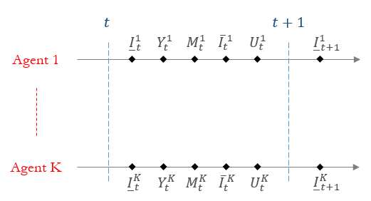
We summarize below the sequence of activities taken by agent $k\in\mathcal{K}$ at time $t$ (Fig. 1):

1. 1.

   The state $X_{t}$ is updated based on (2).

2. 2.

   Agent $k$ receives information from all agents in $\mathcal{K}$, collectively denoted by $\underline{I}_{t}^{k}$.

3. 3.

   Agent $k$ makes an observation about the state $Y_{t}^{k}$ based on (3).

4. 4.

   Agent $k$ updates its memory, $M_{t}^{k}$, defined in Section II-D, on a given protocol.

5. 5.

   Agent $k$ transmits information denoted by $\overline{I}_{t}^{k}$ to every agent $j\in\mathcal{K}$ through the shortest path $q_{{a}}^{[k,j]}$.

6. 6.

   Agent $k$ generates a control action $U_{t}^{k}$.

The information structure of the system is characterized by the graph topology and delays along communication paths described in Section II-A. In the word-of-mouth information structure, every agent $j\in\mathcal{K}$ at time $t$ transmits the information $\overline{I}_{t}^{j}:=\{Y_{t}^{j},U_{t-1}^{j}\}$ to every other agent in the network through the relevant information paths. Agent $k\in\mathcal{K}$ receives information $\overline{I}_{t}^{j}$ at time $t+d^{[j,k]}$, where $d^{[j,k]}$ is the communication delay from $j$ to $k$. Then, the information available to agent $k$ at time $t$ is the collection of information he received from every agent $j\in\mathcal{K}$ at time steps $0$ through $t$.

At time $t$, agent $k$ accesses his memory $M_{t}^{k}$ to generate a control action, namely,

where $g_{t}^{k}$ is the control policy of agent $k$ at time $t$. We define the control policy for each agent as $\bm{g}^{k}:=(g_{0}^{k},\ldots,g_{T}^{k})$ and the control policy of the system as $\bm{g}:=(\bm{g}^{1},\ldots,\bm{g}^{K})$. The set of all feasible control policies is denoted by $G$.

The performance criterion for the system is given by the total expected cost:

where the expectation is with respect to the joint probability measure on the random variables $\{X_{t},U_{t}^{1},\ldots,U_{t}^{K}\}$.

The optimization problem is to select the optimal control policy $\bm{g}^{*}\in G$ that minimizes the performance criterion in (6), given the probability distributions of the primitive random variables $\{X_{0},W_{0:T},V_{0:T}^{1},\ldots,V_{0:T}^{K}\}$, and functions $\left\{c_{t},f_{t},h_{t}^{k}:t\in\mathcal{T},\,k\in\mathcal{K}\right\}$.

For an agent $k\in\mathcal{K}$, we consider a scenario where the control action $U_{t}^{k}$ is generated in two stages:

(1) Agent $k$ generates a function based on information which is a subset of the information available in its memory $M_{t}^{{k}}$.

(2) This function takes as an input the compliment of the subset used to generate it, and yields the control action $U_{t}^{{k}}$.

We call these functions prescriptions. They allow us to construct an optimization problem of selecting the optimal prescription strategy that is equivalent to the problem of selecting the optimal control policy $\bm{g}^{*k}$ as we show next. In this section, we construct the subset of the memory $M_{t}^{{k}}$ and prescriptions for every agent ${{k}}\in\mathcal{K}$ without changing the information structure of the system. In order to simplify the notation, we first define the set of agents located beyond agent $k$ in the set of all agents.

Now we can define the information used to generate prescriptions.

For example, we can write (7) for agent $1$ as

and for agent $2$ as

Based on Definition 6, the accessible information $A_{t}^{{k}}$ has the following properties:

where $\mathcal{B}^{{k}}$ is the set of agents beyond ${{k}}$. Property (10) motivates the introduction of a new term to denote the new information added to accessible information $A_{t}^{{k}}$ at time $t$.

We observe in (11) that the accessible information $A_{t}^{{j}}$ of any agent ${{j}}\in\mathcal{B}^{{k}}$ is a subset of the memory $M_{t}^{{k}}$. Thus, we can define the inaccessible information of the agent ${{k}}$ with respect to the accessible information $A_{t}^{{j}}$ for every ${{j}}\in\mathcal{B}^{{k}}$.

The pair of sets $A_{t}^{{j}}$ and $L_{t}^{[{{k}},{{j}}]}$ forms a partition of the set $M_{t}^{{k}}$, such that

As an example, consider a system with three agents Fig. 2. In this system, we have

For agents $2$ and $3$, we can derive similar relationships as illustrated in Fig. 2.

Next, we use these partitions of the memory to define the prescription function.

Every prescription function $\Gamma^{[{{k}},{{j}}]}$ is generated as follows

where we call ${\psi}_{t}^{[{{k}},{{j}}]}$ the prescription strategy of the agent ${{k}}$ for the agent ${{j}}$ given by the mapping

We call $\bm{\psi}^{{k}}:=(\bm{\psi}^{[{{k}},{{1}}]},\ldots,\bm{\psi}^{[{{k}},{{K}}]})$ the prescription strategy of the agent ${{k}}$. The set of feasible prescription strategies for the agent ${{k}}$ is denoted by $\Psi^{{k}}$.

Next, we define the complete prescription of an agent ${{k}}$ below.

The complete prescription for agent ${{k}}$ is constructed as $\Theta_{t}^{{k}}=(\Gamma_{t}^{[{{k}},{{1}}]},\ldots,\Gamma_{t}^{[{{k}},{{K}}]})$.

In this section we present the relationships between the different prescriptions and control policies. The first result states that for an agent $k\in\mathcal{K}$ we can use the complete prescription $\Theta_{t}^{{k}}$ to generate control action $U_{t}^{k}$ instead of the control policy $g_{t}^{k}$.

Similarly, for any prescription strategy $\bm{\psi}^{{k}}$, we can construct an appropriate control policy $\bm{g}$ that generates the same control actions $U_{t}^{{k}}$ for all agents in $\mathcal{K}$.

Lemmas 1 and 2 imply that the control action $U_{t}^{{k}}$ of every agent $k\in\mathcal{K}$ generated through a prescription strategy $\bm{\psi}^{{k}}$, can also be generated through an appropriate policy $\bm{g}$ and vice versa.

Next we show the existence of a positional relationship $e^{[{{j}},{{k}}]}$ from any agent ${{k}}\in\mathcal{K}$ to every agent ${{j}}\in\mathcal{K}$ with desirable properties that allow us to construct optimal control policies of all agents from the optimal prescription strategy of just one agent. The following result establishes that using a positional relationship $e^{[{{j}},{{k}}]}=(e_{1}^{[{{j}},{{k}}]},\ldots,e_{T}^{[{{j}},{{k}}]})$, an agent ${{j}}$ can derive the prescription strategy for agent ${{i}}\in\mathcal{K}$, when given the prescription strategy of agent ${{k}}$ for agent ${{i}}$, namely

To this end, we consider a positional relationship function $e^{[{{j}},{{k}}]}$ from every ${{k}}\in\mathcal{K}$ to every position ${{j}}\in\mathcal{K}$ which satisfies the properties in Lemmas 3 and 4. This implies that for any two agents ${{k}}$ and ${{j}}$, we have the relation,

Lemmas 1 through 4 lead to (41). This implies that the control action $U_{t}^{j}$ for agent $j\in\mathcal{K}$ can be equivalently obtained through the prescription function ${\Gamma}_{t}^{[{{k}},{{j}}]}$ of any other agent ${{k}}\in\mathcal{K}$, if the corresponding inaccessible information is available. Using (41), we can write the cost incurred by the system at time $t$ as

We can then reformulate Problem 1 in terms of the prescription strategy of any agent ${{k}}$. The optimization problem is to select the optimal prescription strategy $\bm{\psi}^{{*k}}\in\Psi^{{k}}$ that minimizes the performance criterion given by the total expected cost:

The task of deriving optimal prescription strategy $\bm{\psi}^{{*k}},$ and subsequently, the complete prescription $\Theta_{t}^{{k}}$ for agent ${{k}}$ is assigned to a fictitious designer that can only access memory $M_{t}^{{k}}$. Note that this maintains the decentralized nature of the problem as the strategies are implemented by the agents in real time with asymmetric and incomplete information. Now, we show the equivalence between the two problems.

Next, we present a state sufficient for input-output mapping in Problem 2 for agent ${{k}}$ following the exposition presented in [33].

From the designer’s point of view, the system behaves as a Partially Observed Markov Decision Process (POMDP) with state $S_{t}^{{k}}$, control input $\Theta_{t}^{{k}}$, output $Z_{t}^{{k}}$ (with $Z^{{k}}_{0:t}=A^{{k}}_{t}$) and cost $\hat{c}^{{k}}_{t}(S^{{k}}_{t},\Theta^{{k}}_{t})$ at time $t$. The difference is that the prescription functions $\Gamma_{t}^{[{{k}},{{j}}]}$, ${{j}}\in\mathcal{B}^{{k}},$ are generated as functions of the accessible information $A_{t}^{{j}}$ instead of $A_{t}^{{k}}$. Thus, structural results for POMDPs cannot be directly applied to Problem 2. Before proceeding to structural results, we define the information state for agent ${{k}}$.

Due to space limitation, the proofs of the following three properties are omitted but can be found in [35]. The first property establishes that the information state $\Pi_{t}^{{k}}$ is independent from the prescription strategy $\bm{\psi}^{{k}}$.

The second property of the information state $\Pi_{t}^{{k}}$ is that its evolution is Markovian.

The third property of the information state $\Pi_{t}^{{k}}$ is that the expected cost incurred by the system at time $t$ can be written as a function of $\Pi_{t}^{{k}}$.

In Lemmas 7 through 9, we established that the information state $\Pi_{t}^{{k}}$ evolves as a controlled Markov chain with control inputs $\Theta_{t}^{{k}}$.

We start by presenting a structural result for agent $K$. By definition, the set of agents beyond agent $K$ contains only agent $K$, i.e., $\mathcal{B}^{K}=\{K\}$. Using (17), this implies that for all agents ${{k}}\in\mathcal{K}$, the prescription component $\Gamma^{[{{K}},{{k}}]}_{t}$ is a function of the accessible information $A_{t}^{{[K]}}$. This leads to the following result derived in [23] through the common information approach.

We know that for any two agents ${{k}}\in\mathcal{K}$ and ${{j}}\in\mathcal{B}^{{k}}$, we have $A_{t}^{{j}}\subset A_{t}^{{k}}$. Given the accessible information $A_{t}^{{k}}$ and the optimal prescription strategy $\bm{\psi}^{*{{k}}}$, agent ${{k}}$ can derive the optimal complete prescriptions $\Theta_{t}^{*{{j}}}$ for every ${{j}}\in\mathcal{B}^{{k}}$. This leads to the following structural result, proved in [35].

References

- [1] A. A. Malikopoulos, “Centralized stochastic optimal control of complex systems,” in Proceedings of the 2015 European Control Conference, pp. 721–726, 2015.
- [2] A. A. Malikopoulos, “Equilibrium Control Policies for Markov Chains,” in 50th IEEE Conference on Decision and Control and European Control Conference, pp. 7093–7098, 2011.
- [3] A. A. Malikopoulos, “A duality framework for stochastic optimal control of complex systems,” IEEE Transactions on Automatic Control, vol. 61, no. 10, pp. 2756–2765, 2016.
- [4] P. R. Kumar and P. Varaiya, Stochastic Systems: Estimation, Identification and Adaptive Control. Upper Saddle River, NJ, USA: Prentice-Hall, Inc., 1986.
- [5] A. A. Malikopoulos, C. G. Cassandras, and Y. J. Zhang, “A decentralized energy-optimal control framework for connected automated vehicles at signal-free intersections,” Automatica, vol. 93, no. April, pp. 244–256, 2018.
- [6] A. A. Malikopoulos, C. Charalambous, and I. Tzortzis, “The average cost of markov chains subject to total variation distance uncertainty,” in Systems & Control Letters, vol. 120, pp. 29–35, 2018.
- [7] C. Amato, G. Chowdhary, A. Geramifard, N. K. Ure, and M. J. Kochenderfer, “Decentralized control of partially observable Markov decision processes,” in Decision and Control (CDC), 2013 IEEE 52nd Annual Conference on, pp. 2398–2405, 2013.
- [8] A. A. Malikopoulos, V. Maroulas, and J. XIong, “A multiobjective optimization framework for stochastic control of complex systems,” in Proceedings of the 2015 American Control Conference, pp. 4263–4268, 2015.
- [9] A. Mahajan, N. C. Martins, M. C. Rotkowitz, and S. Yüksel, “Information structures in optimal decentralized control,” in 2012 IEEE 51st IEEE Conference on Decision and Control (CDC), pp. 1291–1306, IEEE, 2012.
- [10] H. Witsenhausen, “On the structure of real time source coders,” Bell Syst. Tech. J, vol. 58, no. 6, pp. 1437–1451, 1979.
- [11] P. Varaiya and J. Walrand, “Optimal Causal Coding-Decoding Problems,” Math. Oper. Res. Bell Syst. Tech. J. Bell Syst. Tech. J, vol. 59, no. 8, pp. 814–820, 1983.
- [12] A. Nayyar and D. Teneketzis, “On jointly optimal real-time encoding and decoding strategies in multi-terminal communication systems,” in Proceedings of the IEEE Conference on Decision and Control, pp. 1620–1627, 2008.
- [13] D. Teneketzis and P. Varaiya, “The Decentralized Quickest Detection Problem,” IEEE Transactions on Automatic Control, vol. 29, no. 7, pp. 641–644, 1984.
- [14] V. V. Veeravalli, T. Başar, and H. V. Poor, “Decentralized Sequential Detection with a Fusion Center Performing the Sequential Test,” IEEE Transactions on Information Theory, vol. 39, no. 2, pp. 433–442, 1993.
- [15] P. Varaiya and J. Walrand, “Causal coding and control for Markov chains,” Systems and Control Letters, vol. 3, no. 4, pp. 189–192, 1983.
- [16] Y.-C. Ho and K.-C. Chu, “Team decision theory and information structures in optimal control problems–Part I,” IEEE Transactions on Automatic Control, vol. 17, no. 1, pp. 15–22, 1972.
- [17] Y.-C. Ho and K.-C. Chu, “Team decision theory and information structures in optimal control problems-part II,” IEEE Trans. Autom. Control, vol. 17, pp. 22–28, 1972.
- [18] H. S. Witsenhausen, “A standard form for sequential stochastic control,” Mathematical Systems Theory, vol. 7, no. 1, pp. 5–11, 1973.
- [19] A. Nayyar, T. Başar, D. Teneketzis, and V. V. Veeravalli, “Optimal Strategies for Communication and Remote Estimation With an Energy Harvesting Sensor,” IEEE Transactions on Automatic Control, vol. 58, no. 9, pp. 2246–2260, 2013.
- [20] A. Mahajan and D. Teneketzis, “On the design of globally optimal communication strategies for real-time noisy communication systems with noisy feedback,” IEEE Journal on Selected Areas in Communications, vol. 26, no. 4, pp. 580–595, 2008.
- [21] J. Wu and S. Lall, “A dynamic programming algorithm for decentralized markov decision processes with a broadcast structure,” in 49th IEEE Conference on Decision and Control (CDC), pp. 6143–6148, IEEE, 2010.
- [22] A. Nayyar, A. Mahajan, and D. Teneketzis, “Decentralized stochastic control with partial history sharing: A common information approach,” IEEE Transactions on Automatic Control, vol. 58, no. 7, pp. 1644–1658, 2013.
- [23] A. Nayyar, A. Mahajan, and D. Teneketzis, “Optimal control strategies in delayed sharing information structures,” IEEE Transactions on Automatic Control, vol. 56, no. 7, pp. 1606–1620, 2011.
- [24] A. Mahajan, “Optimal decentralized control of coupled subsystems with control sharing,” IEEE Transactions on Automatic Control, vol. 58, no. 9, pp. 2377–2382, 2013.
- [25] A. Nayyar, A. Gupta, C. Langbort, and T. Basar, “Common information based markov perfect equilibria for stochastic games with asymmetric information: Finite games,” IEEE Transactions on Automatic Control, vol. 59, no. 3, pp. 555–570, 2014.
- [26] J. Arabneydi and A. Mahajan, “Team optimal control of coupled subsystems with mean-field sharing,” in 53rd IEEE Conference on Decision and Control, pp. 1669–1674, Dec 2014.
- [27] S. M. Asghari, Y. Ouyang, and A. Nayyar, “Optimal local and remote controllers with unreliable uplink channels,” IEEE Transactions on Automatic Control, vol. 64, no. 5, pp. 1816–1831, 2018.
- [28] S. Yuksel, “Stochastic nestedness and the belief sharing information pattern,” IEEE Transactions on Automatic Control, vol. 54, no. 12, pp. 2773–2786, 2009.
- [29] T. Yoshikawa, “Decomposition of dynamic team decision problems,” IEEE Transactions on Automatic Control, vol. 23, no. 4, pp. 627–632, 1978.
- [30] M. Aicardi, F. Davoli, and R. Minciardi, “Decentralized optimal control of markov chains with a common past information set,” IEEE Transactions on Automatic Control, vol. 32, no. 11, pp. 1028–1031, 1987.
- [31] G. Casalino, F. Davoli, R. Minciardi, P. Puliafito, and R. Zoppoli, “Partially nested information structures with a common past,” IEEE transactions on automatic control, vol. 29, no. 9, pp. 846–850, 1984.
- [32] A. Dave and A. A. Malikopoulos, “Decentralized stochastic control in partially nested information structures,” in 8th IFAC Workshop on Distributed Estimation and Control in Networked Systems, 2019 (to appear).
- [33] A. Mahajan, Sequential Decomposition of Sequential Dynamic Teams: Applications to Real-Time Communication and Networked Control Systems. PhD thesis, University of Michigan, 2008.
- [34] H. Witsenhausen, “Some remarks on the concept of state,” in Directions in Large-Scale Systems, pp. 69–75, Springer, 1976.
- [35] A. Dave and A. Malikopoulos, “The prescription approach to decentralized stochastic control with word-of-mouth communication,” arXiv e-prints, p. arXiv:1907.12125, Sep 2019.
- [36] A. Mahajan and S. Tatikonda, “An algorithmic approach to identify irrelevant information in sequential teams,” Automatica, vol. 61, pp. 178–191, 2015.