Co-simulation of Continuous Systems: A Tutorial
1 Introduction
Truly complex engineered systems that integrate physical, software and network aspects are emerging [23], posing challenges in their design, operation, and maintenance.
The design of such systems, due to market pressure, has to be concurrent and distributed, that is, divided between different teams and/or external suppliers, each in its own domain and each with its own tools [34]. Each participant develops a partial solution, that needs to be integrated with all the other partial solutions. The later in the process the integration is done, the higher its cost [26]. Ideally, the solutions developed independently should be integrated sooner and more frequently, in so-called full system analysis [33].
Modeling and simulation has improved the development of the partial solutions, but falls short in fostering this holistic development process [4]. To understand why, one has to observe that:
(i) models of each partial solution cannot be exchanged or integrated easily, because these are likely developed by a specialized tool; (ii) externally supplied models may have Intellectual Property (IP) that cannot be cheaply disclosed to system integrators; (iii) as solutions are refined, the system should be evaluated by integrating physical prototypes, software components, and even human operators, in what are denoted as Model/Software/Hardware/Human-in-the-loop simulations [1]; and (iv) the models of each partial solution have different characteristics that can be exploited to more efficiently simulate them, making it difficult to find a technique that fits all kinds of models.Co-simulation is a generalized form of simulation, where a coupled system is simulated through the composition of simulation units [17, 19, 25]. Each unit is broadly defined as a black box capable of exhibiting behaviour, consuming inputs and producing outputs, over simulated time.
Many of the problems occurring in co-simulations are due to the ill composition of simulation units that represent continuous systems [16]. As such, we argue that having a basic knowledge of numerical (co-)simulation can help practitioners debug, and even improve the performance of, existing co-simulations.
In this tutorial, we aim to provide the reader with a basic understanding of numerical algorithms, and we show how attempting to simulate an heterogeneous system naturally leads to co-simulation. Upon completion, the reader should know the many different possible co-simulation approaches, the main concepts involved, and what their tradeoffs are. Furthermore, the reader will be equipped to understand the more advanced concepts in the co-simulation literature.
The next section provides a top-down overview of all the concepts that will be discussed here. This concept map will be revisited in all other sections. In the sections after, each concept will be discussed, in a bottom up manner, so as to increase the complexity gradually.
2 Main Concepts
In this section, we will provide an informal top-down overview on the concepts related to co-simulation. To that end, we will use a feature model [20]: an intuitive diagram that breaks down the main concepts in a domain. Some of these concepts will only become clear in later sections, as we delve into the details, so we recommend the reader to come back to this section to place these in the grand scheme of things. More rigorous definitions are given in [17].
First, we summarize the objective of running a co-simulation: to reproduce, as accurately as possible, the behavior of a system under study.
Figure 1 breaks down the main concepts in the co-simulation domain. To run a co-simulation, one needs a co-simulation scenario and an orchestrator algorithm.
The co-simulation scenario points to one or more simulation units, describes how the inputs and outputs of their models are related, and includes the configuration of relevant parameters.
Each simulation unit represents a black box capable of producing behavior. To produce behavior, the simulation unit needs to have a notion of:
- •
a model, created by the modeller based on his knowledge of the system under study;
- •
a solver, which is part of the modeling tool used by the modeller, that approximates the behavior of the model; and
- •
an input approximation, which approximates the inputs of the model over time, to be used by the solver;
- •
input reactivity and output reactivity, that determine which inputs the simulation unit receives from the orchestrator.
The orchestrator is responsible for running the co-simulation. It initializes all the simulation units with the appropriate values, sets/gets their inputs/outputs, and coordinates their progression over the simulated time. To progress the co-simulation, the orchestrator, after setting the appropriate inputs to the simulation units (computed from their outputs according to the co-simulation scenario), asks them to simulate for a given interval of simulated time, by providing them with a communication step. The simulation units in turn will approximate the behavior of their model within the interval between the current simulated time and the next communication time, relying only on the inputs they have received at the previous communication times. In order to simplify the explanations and analyses presented later in this document, we assume that the simulation units will only receive more inputs at the next communication with the orchestrator, hence they must rely on their input approximations.
Figure 2 gives an illustration of these concepts. The figure in the left-hand side illustrates how the orchestrator coordinates the co-simulation by getting outputs, setting inputs, and requesting the simulation units S1 and S2 to progress in time. The figure in the top-right-hand side presents the co-simulation scenario, where receives input and outputs , and receives inputs and outputs . The two figures in the bottom-right-hand side presents the internal behaviour of the simulation units. The large unfilled dots represent input values, and the smaller unfilled dots represent their extrapolations, as computed by the simulation units. One can see that there is a difference between the values calculated by the extrapolation functions opposed to the actual input, due to the gap between the larger and smaller unfilled dots at . The black dots represents outputs. As illustrated, and perform small steps of respectively and internally, until the time is reached.
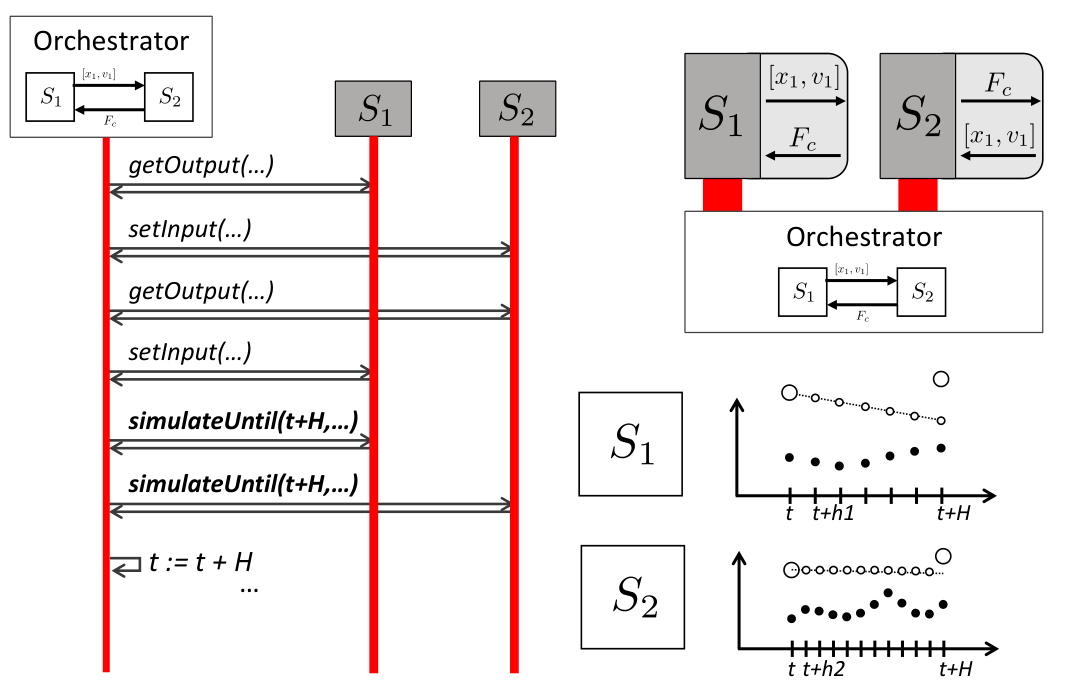
The communication step size can either be fixed (defined before the co-simulation starts and constant throughout its execution), or adaptive (the orchestrator determines the best value to be used whenever it asks the simulation units to compute).
The communication approach encodes the order in which the simulation units are given inputs and instructed to compute the next interval. Figure 3 summarizes the multiple types of orchestration algorithms using time diagrams.
In the Gauss-seidel approach, the orchestrator asks one simulation unit at a time to compute to the next interval and produce outputs. Then, the orchestrator uses the most recent outputs when asking the next unit to compute.
In the Jacobi approach, the orchestrator asks all units to compute the interval in parallel, setting their inputs at the end of the co-simulation step.
Finally, the orchestrator may retry the co-simulation step, using improved input estimates, computed from the most recent outputs. This process can be repeated until there is no improvement on the inputs (fully implicit iteration), or a fixed number of iterations has been done (semi-implicit iteration). In the later sections it will become clear why it is a good idea to retry the co-simulation step.
In the following sections, we will follow a bottom up approach, starting with the simplest concepts in Figure 1, and building our way up to co-simulation.
3 Models, Solvers, and Input Approximations
Since co-simulation is a form of generalized simulation, it is paramount that simulation is well understood. In this section, we cover the basic algorithms to approximate the solution, , of first order Ordinary Differential Equations (ODEs), , having an initial condition, . We start with scalar differential equations and then move to vector equations. A running example will be incrementally constructed, so that the numerical methods introduced can be tried out.
The relationship between the concepts learned in Sections 3.1 and 3.2, and the concept of simulation unit (recall Figure 1), is discussed in Section 3.3.
3.1 Scalar Initial Value Problems
A scalar Initial Value Problem (IVP) is defined as a scalar ODE, with an initial condition. Formally, it has the form:
| (1) |
where denotes the (scalar) state function, denotes the time derivative of , is a scalar function, is the input function, and is a given initial value of .
Example 1.
Consider a car whose acceleration is set by a cruise controller, and moves in a straight line. Let denote the speed of the car over time, its mass, and the desired speed (input); and assume that the car is initially moving at speed . Then the scalar IVP is given by
| (2) |
where is the acceleration set by the cruise controller, is the input, is the acceleration multiplier constant, and is the friction coefficient.
The solution of the scalar IVP (1) is a function whose derivative satisfies Equation 1. For example, the solution of the IVP posed in the car example (Example 1), and plotted in Figure 4, is:
In general, it is not possible, nor feasible, to find an explicit solution to the IVP. Instead, an approximate solution can be computed using a numerical method. In the following, we provide an intuitive derivation of two variations of Euler’s method.
To derive an approximation of the solution to the scalar IVP in Equation 1, we start by noting that the initial point is given by the initial value, that is, , so at least one point is known. For a small , the limit definition of the derivative in the left hand side of Equation 1 can be replaced by its approximation . By Equation 1, we have , which can be solved for to give the Explicit Euler Method:
| (3) |
Applying Equation 3 to the initial value, gives the point , which approximates . The procedure can then be repeated using to compute , and so on. This method can be applied to the car example by combining Equation 2 and Equation 3:
| (4) |
The approximation calculated by Equation 4 with the parameters: is shown in Figure 4, i.e., the speed at time is calculated by:
| (5) |
The implicit variation of Euler’s method is derived in the same way as the explicit variation. The difference is that instead of deriving the method from the approximation , we evaluate at the point . That is, we take the approximation , and rearrange it to get the Implicit Euler Method:
| (6) |
The value of is the unknown in Equation 6, and depends on itself, that is, it appears on both sides of the equation, creating an algebraic loop. We now present a simple method to estimate in Equation 6.
The direct iteration method11 1 The direct iteration method is also known as successive substitution, functional iteration, or fixed point iteration., computes the solution to an equation by starting from an initial guess denoted as and evaluating the right hand side with it. Then the result is used for the next evaluation of the right hand side, until two successive evaluations are close enough. In other words, it computes the iteration
| (7) | ||||
When applying the direct iteration method as part of a simulation step of the implicit Euler method, a good initial guess can be given by the most recently computed value or by an application of the explicit Euler step. Formally, at simulation time , , or .
Example 2.
To demonstrate direct iteration, the implicit Euler method presented in Equation 6 can be applied to Equation 2 to get:
| (8) |
Table 1 presents the results of two steps with Equation 8 ( and ), using the implicit euler method with the parameters as in Equation 5. Each step comprises five iterations of the direct iteration method. The value from the last iteration in the first step is used as the initial guess in the second step. The initial guess in the first step is the result of one explicit Euler step as in Equation 5: . The values in bold represent the result of the implicit euler step.
| Initial Guess | 1 | 2 | 3 | 4 | 5 | |
|---|---|---|---|---|---|---|
| 5 | 4.4413 | 4.5122 | 4.5032 | 4.5044 | 4.5042 | |
| 4.5042 | 9.0085 | 8.4366 | 8.5092 | 8.5000 | 8.5012 |
The direct iteration method will converge to a solution if successive results get closer and closer, as illustrated in Figure 5. Formally, that means that
| (9) |
is satisfied for every . In the case that , then the solution has converged.

Example 3.
Applying Equation 9 to the values in Table 1 results in the values in Table 2, which shows convergence as every value is smaller than 1.
| 1 | 2 | 3 | 4 | |
|---|---|---|---|---|
| 0.1270 | 0.1270 | 0.1270 | 0.1270 | |
| 0.1270 | 0.1270 | 0.1270 | 0.1270 |
Now we derive a condition which is stronger than the above condition, but can be used to predict whether convergence will occur, without actually having to compute the iteration. By the Mean Value Theorem, there exists a such that
The condition
can be satisfied for all if we require that
| (10) |
Equation 10 shows us that the direct iteration method, when used in combination with the implicit Euler method (Equation 6), is always guaranteed to converge, provided that the step size used is small enough. To see why, let denote the direct iteration function, where and are known, and is the unknown. Differentiating with respect to , taking the absolute, and adding the restriction in Equation 10, yields
| (11) |
Applying the above equation to Equation 2, with the parameters in Figure 4, yields , which means must satisfy .
Figure 4 shows the approximation computed with the Implicit Euler method.
3.2 Vector Initial Value Problems
In this sub-section, we generalize the numerical techniques introduced in Section 3.1 to vector IVPs. We will denote vectors with bold face, and we will use capital letters for matrices and vector valued functions. Given a vector , we denote its transpose as . Furthermore, we denote the -th element of vector by , so that . Similarly, denotes the -th element of the vector returned by .
An Initial Value Problem is the generalization of Equation 1, to vectors:
| (12) |
where and are vector functions, and is a vector valued function.
Example 4.
The mass-spring-damper system, illustrated in Figure 6, is modelled by the following second order ordinary differential equation:
where denotes the position of the mass, is the stiffness coefficient of the spring, is the damping constant of the damper, and denotes an external force exerted on the mass.
The above equation can be put into the form of Equation 12 by introducing a new variable for velocity, , and letting the vector . Given an initial position and velocity , we obtain the following IVP:
The time derivative of a vector is the time derivative of each of its components, so the solution to Equation 12 is a vector valued function where each component obeys the equation , with . As an example, Figure 7 shows the solution of the position component of the mass-spring-damper IVP introduced in Example 4. The solution to the velocity component is omitted.
The Explicit Euler Method can be derived as follows. Taking the limit definition of the derivative of , and rearranging as done to obtain Equation 3, we get , for a small . This equation, applied to all components of , can be put in matrix form:
| (13) |
The Implicit Euler Method can be derived analogously:
| (14) |
The condition in Equation 11 for convergence of the direct iteration (Equation 7) used in combination with the implicit Euler method (Equation 14), also generalizes to the vector IVP (Equation 12) by replacing the absolute by a vector norm . It is a special case of the Contraction Mapping Theorem [24, Theorem 8.2.2].
3.3 Constructing Simulation Units
This subsection describes how the concepts introduced in the previous subsection can be used to construct simulation units.
Models are vector IVPs with output:
| (15) | ||||
where denotes the output vector, and the output function.
Solvers are numerical methods, such as the Euler methods introduced in Equations 13 and 14.
To understand the role of input extrapolation functions, we need to recall the interactions between the orchestrator and each simulation unit (recall Figure 2).
In order to facilitate the explanation, let us make the following assumptions: denotes the communication step size, kept the same throughout the co-simulation; denotes the simulated time at the -th co-simulation step; and the orchestrator follows a Jacobi approach (see Figure 3). The other cases should be easy to understand once this one is clear.
Under the above assumptions, the orchestrator, at time , constructs the input to the unit, denoted as , and then asks the unit to compute until the time .
Between times and , the unit will iteratively approximate the state of the model, only taking into account the inputs that it has received in the past. As such, the numerical solver employed in the simulation unit is actually solving a modified version of Equation 15:
| (16) |
where is an approximation of in the interval , built from input samples computed by the orchestrator in the previous co-simulation steps: , , , ….
In this interval, the goal of the simulation unit is to estimate , so that the output of the model (recall Equation 15) can be computed and given to the orchestrator. Since the output at time may depend on the input at time , it can be estimated in two ways, depending on the output reactivity of the simulation unit:
- Output reactive:
-
using the input given by the orchestrator, that is,
- Output delayed:
-
using the approximation of the input, that is,
Regardless of how the output is computed, it can be the case that the numerical method being used internally in the simulation unit from time to , is implemented in a way that requires the availability of the input at time . Formally, this means the state at the next communication time is estimated as
| (17) |
where encodes the construction of the input extrapolation function, and the iterative application of the numerical method, starting from state until state . The units employing these methods are denoted as input reactive.
In contrast, simulation units are input delayed when they do not require the input at time in order to estimate :
| (18) |
Table 3 summarizes the types of simulation units.
| Output Reactive | Output Delayed | |
|---|---|---|
| Input Reactive | ||
| Input Delayed |
Note that the kind of simulation unit may impose a specific interaction pattern with the orchestrator. For example, simulation units that are input reactive cannot be interacted with with a Jacobi approach. The formal definition of simulation units will be given in Section 4.4, when a more rigorous definition of co-simulation scenario is given.
3.4 Summary and Further Reading
This section presented the most basic numerical methods for the simulation of IVPs. For an introduction to more advanced methods, we recommend [9], and for an in-depth mathematical treatment of these, we recommend [35]. For an overview of modeling with differential equations, see [8]. For an introduction to dynamical systems modeling and simulation, see [32].
Methods for solving equations of the form , such as the successive substitution method, are given in, e.g., [5, Chapter 2]. The alternative derivations of the Euler method, see [11, Section 5.2]. More details about the derivation of Equation 10 can be found in [5, Theorem 2.4], and its generalization can be found in [24, Theorem 8.2.2]. The formal definitions of simulation units, and their types, are based in [15].
4 Basics of Co-simulation
In this section, we show how co-simulation arises naturally out of the need to use specialized numerical methods for different parts of a given IVP. To exemplify this, we start by introducing a running example. Then, after showing that it is difficult to simulate the running example using the previously introduced numerical methods, we introduce a new numerical method that can be used to simulate only a part of the example. Then we introduce co-simulation as a technique that allows the new numerical method to be combined with the previous ones. Finally, we provide an overview of more advanced techniques that can improve the co-simulation.
4.1 Motivating Example
Inspired by the work in [2], we intend to simulate the forces on the body of a passenger in a moving car. To keep it simple22 2 For more details about modeling the human body, see [9, Chapter 5] for an introduction, and [2]., and to combine the models already introduced in Examples 1 and 4, we model the passenger as two coupled mass-spring-damper systems, representing the head and torso, and the vibrations of the motor as a mass-spring system.
Example 5.
The IVP of a passenger in an accelerating car, illustrated in Figure 8, is given by:
| (19) | ||||
where the initial and parameter values are:
| (20) | ||||
The model introduced in the above example can be put in matrix form as in Equation 29. Therefore, its analytical solution can be computed as detailed in Section B.1. The analytical solution, along its approximation computed with the explicit Euler, is shown in Figure 9.
Clearly, the approximation for this example is not satisfactory. This is because the explicit Euler method is not appropriate to simulate the motor sub-system. To see why, note that the equations governing in Example 5 are the same as the ones introduced in Example 8, with and , which means that the Euler method is numerically unstable for this subsystem.
4.2 Specialized Numerical Methods
The mass-spring is part of a more general class of problems called second derivative IVPs.
Second derivative IVPs have the form:
| (21) |
and these typically show up in IVPs over equations modeling physical systems where energy is conserved [9, Chapter 5].
Instead of converting the above IVP to a first order one (as illustrated in Example 4), there are numerical methods that take advantage of the special structure of this problem.
Godunov’s method computes the approximated solution to the second derivative IVP in Equation 21 using the following iteration:
| (22) |
where is given. At time , this method requires access to two previously computed approximations ( and ), which it can only be used from onward. Fortunately, at this time, the value can be computed using other numerical methods. Godunov’s method is an example of a multi-step numerical method [35, Chapter III].
As an example, the bottom plot of Figure 11 shows the motor vibrations computed with Godunov’s method.
Despite the good performance of Godunov’s method to simulate the mass-spring subsystem of Example 5, it cannot be used as is to simulate the complete IVP33 3 It is possible to adapt Godunov’s method to simulate IVPs that involve the first derivative (see, e.g., [9, Section 5.5])., as it does not have the form of Equation 21. In the following sub-sections, we show how to decouple the example into sub-problems, and solve each with the most appropriate numerical method.
4.3 Decoupling IVPs
In the light of the concepts introduced earlier, we can refine the definition of the concepts in Figure 1.
Here, we define Co-simulation as a technique to couple numerical methods, each responsible for a part of the given IVP, in order to approximate the solution to that IVP.
The configuration of the co-simulation scenario is an assignment of values to the parameters that affect the co-simulation execution. For example, one such parameter is the co-simulation step size , which controls the points in time at which the numerical methods will exchange values (i.e., at multiples of ). The concrete set of parameters depend on the co-simulation orchestrator so we do not detail them here. Each model represents an IVP, and all models represent a decomposition of the system under study, which we consider to be an IVP as well44 4 There are examples of co-simulations where the original model is not an IVP, but instead is a differential algebraic system. See [18, 7, 21, 3]..
Example 6.
An example co-simulation scenario for the IVP introduced in Example 5 is summarized in Figure 10. The vibrations of the car are approximated using the Godunov’s method (Equation 22), and the other two parts are simulated with the Explicit euler method.
4.4 Orchestration
The algorithm that processes the co-simulation scenario and coordinates the execution of the simulation units is called the orchestrator55 5 The orchestrator is also known as the master, or coordinator.. In this sub-section, we introduce the Gauss Seidel and Jacobi orchestration algorithms, named after the analogous techniques to solve linear systems. To explain these methods, we need to first detail the elements that comprise a co-simulation scenario.
Let denote the given communication time step. We denote the -th communication time as . We say that the -th step of the co-simulation is finished when all the numerical methods have computed their solutions up to, and including, time .
Each model is associated with a reference , where is a set of all model names. The model is an IVP with output:
| (23) | ||||
where denotes the output vector, and the output function.
As described in Section 3.3, the input function is an approximation (i.e., extrapolation or interpolation) constructed from samples of the outputs of other models. We will denote the set of models whose output is used to construct the input , as , standing for Source models. With this notation, for , the input is constructed from the samples of the outputs of every model at the current and previous co-simulation steps. The number of samples needed depend on the concrete approximation technique.
We will use to refer both to the model and the simulation unit, when there is no ambiguity.
Roughly, the task of the orchestrator at time is to provide the output samples that each unit needs, and ask the unit to approximate the value of . Therefore, the orchestrator needs to distinguish units according to not only which samples are required to construct their input functions (input reactive or delayed), but also whether their output functions require actual values for inputs or not (output delayed or reactive). We now describe formally each type of simulation units introduced in Table 3.
A unit is input reactive if, at any , there is at least one such that the input depends on the value of at time . Otherwise, is input delayed.
A unit is output reactive if at any time , there is at least one such that the computation of the output requires the value of at . Otherwise, is output delayed. Note that the output function may still depend on the input for a unit that is output delayed: it just means that the unit will employ the input approximation in place of the actual input.
The reactivity properties can be seen as contracts between the simulation units and the orchestration algorithm. These are specific to how the simulation units are implemented, and not to the sub-models themselves. In order words, the same sub-model may be implemented differently in different simulation units.
4.4.1 Gauss-Seidel Orchestrator
With the above classification, the Gauss-Seidel orchestrator can determine which outputs are used to compute which inputs, and at which times. This allows it to sort the execution of the units, so that the output samples on which they depend are always available.
At the -th co-simulation step, a unit must be executed after unit if and is (input or output) reactive.
To keep the orchestrator simple we assume that the units can always be sorted. In Section 4.4.3 we relax this assumption.
We denote the order with a map , that returns the unit reference that is the -th in the order. For example, the unit is the first.
Under these assumptions and notation, the Gauss-Seidel orchestrator is summarized in Algorithm 1. Function computes the input sample of unit from the output samples of its sources. The function asks unit to compute the output, optionally using the value in the variable Likewise, function asks unit , assumed to be in state , to compute the value , using either one of the variables provided, depending on its type (i.e., use if the unit is input reactive, or use otherwise). Any other previous inputs the unit may require are assumed to be stored in its internal state (collected from previous calls to the doStep function.
Figure 11 shows the solution approximated with the co-simulation of Example 6 using Algorithm 1.
4.4.2 Jacobi Orchestrator
The main difference between the Jacobi and Gauss-Seidel orchestrator lies in the fact that the Jacobi orchestrator assumes that every simulation unit is input delayed. This has a couple of consequences:
- •
There is no need to order the units for the execution of the doStep function. However, the units can still be output reactive/delayed, so the invocations of the getOutput functions still need to be sorted.
- •
There is no need to keep track of the previous inputs to each unit.
The Jacobi orchestrator is summarized in Algorithm 2. Compared to the Gauss-seidel orchestrator, the Jacobi is in general less accurate (due to the fact that units cannot use interpolation techniques), but can take advantage of parallelism.
4.4.3 Implicit and Semi-Implicit Orchestrators
The Jacobi and Gauss-Seidel orchestration algorithms have iterative counterparts (recall Figure 1). An iterative orchestration algorithm will retry each co-simulation step multiple times. If the number of repetitions is fixed, then we say that the orchestration is semi-implicit. If, on the other hand, the co-simulation step is repeated until some criteria is met, then the orchestration is implicit.
In general, iterative techniques are useful when the non-iterative techniques fail to preserve the stability of the original IVP, or when there are algebraic loops in the co-simulation scenario. When there are algebraic loops, then the units cannot be sorted, as assumed in Section 4.4.1.
We distinguish two kinds of algebraic loops in co-simulation [17, 21]:
• output loops:the ones spanning just output variables; and • state loops:the ones that include state variables as well.Output loops arise when there is an output of a simulation unit that depends (through the couplings of the co-simulation scenario) on itself, while state loops happen when the state of an input reactive simulation unit depends on itself.
To illustrate these, we introduce a directed graph based notation to represent dependencies. Each vector of outputs/inputs/state is represented as one node. The edges are drawn as follows:
- •
whenever an output vector depends on an input or state vector, an edge is drawn between the corresponding nodes;
- •
when an input depends—through the couplings of a co-simulation scenario—on an output, an edge is drawn between the corresponding nodes.
- •
when the state evolution function uses an input interpolation approximation (that is, when the unit is input reactive), then an edge is drawn between the input node and the state node.
Figure 12 shows an abstract example co-simulation scenario illustrating the different dependencies.
With the dependency relationship introduced, the algebraic loops give rise to cycles in the graph. If a cycle has nodes that correspond to a state vector, then it is a state loop. Otherwise, it is an output loop. These algebraic loops are highlighted in Figure 12.
Algorithm 3 illustrates the iterative version of the Gauss-seidel orchestrator. Function hasConverged encodes the test for convergence, which can either count a fixed number of iterations (semi-implicit method), or check whether the output values have converged (implicit method). The rollback function reverts the state of the simulation unit to the one before the most recent call to the doStep function. Contrarily to its non-iterative counterpart, the order used in this algorithm does not necessarily reflect the dependencies between simulation units: it is merely an order defined by the user.
The iterative version of the Jacobi algorithm is similar, so we omit it.
4.5 Advanced Co-simulation Techniques
In order to simplify the explanation, and to keep the algorithms within one page, we made some assumptions in the previous sub-sections. Additionally, there are more advanced techniques that can be applied in practice to improve the performance of co-simulations. We discuss these in the following.
4.5.1 Initialization
Until now we have assumed that, in a co-simulation scenario, each simulation unit has a given initial state, independent of the initial state of other simulation units. In practice, this might not be the case, so the co-simulation scenario has to include a description of how the initial states are related (see the initial state couplings concept in Figure 1), and the orchestrator has to compute these initial states. This computation is similar to the computation of initial outputs, and may also include algebraic loops.
4.5.2 Fine Grained Input/Output Dependencies
We also assumed that the representation of the dependency information between input, state, and output vectors was adequate. It is better to represent the dependencies between the scalar variables. To see why, observe the example in Figure 13, which shows the same co-simulation scenario as the one in Figure 12, but instead of using the vector level dependency information, it uses the the scalar level. What was identified as an output algebraic loop in Figure 12, is no longer one at the scalar level dependency graph in Figure 13. This is called a virtual algebraic loop and does not require iterative techniques to be solved. The orchestrator then can set the appropriate scalar inputs, and inquire for the scalar outputs, in the right order. Please refer to [3] and [11, Section 3.2] for details on how to represent the graph, compute the topological sort, and identify the algebraic loops.
4.5.3 Input/Output Couplings
4.5.4 Adaptive Communication Step
We assumed that the communication step size has to remain fixed over the co-simulation. In practice, it is often better that the orchestrator varies the communication step size, and/or asks the simulation units to adjust their own numerical method and approximation schemes, in order to respond to external requirements or react to the past dynamics of the co-simulation.
4.6 Summary and Further Reading
This section showed how the specialization of numerical methods naturally leads to the need for co-simulation. Then it defined the intervenients in the co-simulation process and introduced the different kinds of orchestration algorithms. Finally, it discusses some of the advanced techniques.
5 Conclusion
The co-simulation technique introduced in the previous section allows us to apply the best numerical method to each part of a given IVP. This is not the only benefit though.
For example, each numerical method can use a different step size. This is an advantage because different models may evolve with derivatives that are orders of magnitude apart, as is the case in Example 5 where the accelerations measured in the car model are four orders of magnitude lower than the accelerations measured in the psg unit. Therefore, as shown in the co-simulation computed in Figure 11, the car unit can afford to take one simulation step per co-simulation step, while the psg unit takes 100 steps, without drastically affecting the overall accuracy.
Another benefit is that simulation units do not have to disclose the equations being solved internally. Instead, it is common to only disclose the outputs and inputs, capabilities such as the ability to rollback, and the derivatives of outputs with respect to time and inputs. The black box nature of the units makes it easier to standardize their interface, which in turn enables the coupling of mature modeling and simulation tools. Wide industrial adoption is one of the main drivers behind research into co-simulation [28].
This tutorial aims at introducing the main concepts in co-simulation, and providing researchers and practitioners with further reading in each of the topics. The concepts introduced here represent the fundamental concepts in co-simulation, general to any co-simulation framework.
Acknowledgments
This work was executed under the framework of the COST Action IC1404 – Multi-Paradigm Modelling for Cyber-Physical Systems (MPM4CPS), and partially supported by: Flanders Make vzw, the strategic research centre for the manufacturing industry; the INTO-CPS project funded by the European Commission’s Horizon 2020 programme under grant agreement number 664047; and PhD fellowship grants from the Agency for Innovation by Science and Technology in Flanders (IWT, dossier 151067).
We thank Mehrdad Moradi for his comments and suggestions regarding this document.
Appendix A Numerical Stability
In this section, we introduce the concept of stability of a system of ordinary differential equations, and derive the conditions under which the numerical methods introduced in Section 3 preserve this property.
We say that the system of differential equations in Equation 12 is asymptotically stable when all its solutions tend to zero as time passes, regardless of the initial value. Formally, for all satisfying Equation 12.
The following example illustrates why asymptotical stability is an important property.
Example 7.
Consider the solution of the cruise controlled car IVP, introduced in Example 1.
After some time, the velocity of the car will be constant. Let denote this velocity. It can be computed by noting that the acceleration of the car will be zero at that speed. Hence, setting the right hand side of Equation 2 to 0, and rearranging gives .
Determining the stability of Equation 2 allows us to prove that the velocity of car actually tends to , which is an important property of the cruise controller. Let and , so that Equation 2 can be written as , and . Then introduce a new variable representing the difference between the car velocity and the terminal velocity. With the new variable, Equation 2 can be written as . Since , any solution as , independently of , thus proving that the cruise controller is asymptotically stable66 6 Notice that for and . This makes the cruise controller incorrect, but keeps the example simple..
As the previous example shows, a scalar ODE in the form of
| (24) |
is asymptotically stable if . The analogous condition for vector ODEs of the form of
| (25) |
is that the real part of all eigenvalues of is strictly negative [35, Section I.12]. Formally,
| (26) |
Both these conditions can be checked automatically.
To see why a numerical method may fail to preserve the asymptotic stability of a system of differential equations, consider a scalar ODE in the form of Equation 24, and apply the explicit Euler method (Equation 13) to get , where . For any , the term as if . Note that the larger is, the smaller the step size has to be, in order for the method to be numerically stable.
The vector version of the above derivation is analogous. Consider a vector ODE in the form of Equation 25, and apply the explicit Euler method (Equation 3) to get , where . For any , the term as if [30], where denotes the maximum absolute eigenvalue of , also called the spectral radius of . The analogous condition for the implicit Euler is , where is matrix inverse of .
The procedure to decide the numerical stability is summarized as follows. Apply the equation representing the numerical approximation to a differential equation of the form of Equation 25, and obtain an equation with the form
| (27) |
where is a constant matrix. Then check whether .
When the explicit Euler is numerically unstable, a solution is to decrease the step size , as it decreases the quantity . However, as the next example shows, the step size required to obtain a stable solution can be prohibitively small. When this is the case, we recommend the use of a different numerical method, with better stability properties, such as the implicit Euler method.
Example 8.
Consider the mass-spring-damper, introduced in Example 4, with , for any , , and . It can be written in the form of Equation 25, with
The numerical stability of the explicit Euler method with the above equation is determined by . For , this inequality can be simplified to highlight the real and imaginary parts of the left hand side,
Computing the absolute and simplifying gives . As the parameter , the maximum safe step size as well, which means that in the limit where , the explicit Euler method will never preserve the stability property. The same can be observed as the parameter .
A.1 Further reading
Appendix B Approximation Accuracy
In the previous section, we looked at whether a qualitative property of the original IVP could be preserved under a numerical simulation. In this sub-section, we start by introducing a technique to compute the correct solution to a restricted class of differential equations, so that we can later show how to experimentally compute the approximation error of a numerical method, as a function of the step size used.
B.1 Analytical Solution
When the IVP in Equation 12 has the form of Equation 25, the analytical solution is given by
| (28) |
where is the matrix exponential of [10, Section 2.2]. This can be verified by taking the derivative of , and obtaining (the right hand side of the IVP in Equation 12).
Most software libraries include algorithms to approximate the matrix exponential in Equation 28. Furthermore, the computation of can be done incrementally, mimicking a numerical method, by noting that .
The formulation in Equation 28 is generic enough to allow the computation of the solution to equations of the form
| (29) |
where is a constant vector: Equation 29 can be transformed to the form in Equation 25 by introducing a new state vector and solving the IVP
where denotes the null matrix with dimensions .
B.2 Experimental Approximation Error
Given an approximation of the solution to the IVP introduced in Equation 12, we define the approximation error of an approximation computed with step size as , and the maximum error up to a finite as .
We can experimentally plot the error of a numerical method applied to an IVP as a function of the step size as follows. Pick a finite simulation time ; and compute the maximum error of the analytical and numerical solutions up to for different step sizes.
The resulting can be used to get the order of the numerical method. Roughly, for sufficiently small , if for a given function and positive constant , then we say that is in the order of , or in other words, . The constant that approximates the error depends on the IVP being solved, but the order is a property of the numerical method [35, Section I.7 and II.1].
Example 9.
The Midpoint method is given by the iteration:
Figure 14 compares the approximation error of the explicit Euler method (Equation 13) with the approximation error of the Midpoint method, when applied to the IVP introduced in Example 8. The Midpoint method is , while the explicit Euler is . Also note that, for the same maximum error, the step size required by the Midpoint method is larger than the required for the explicit Euler.
B.3 Further Reading
Appendix C Co-simulation Convergence and Stability
The methods introduced in Appendices A and B can be applied to co-simulations as well.
C.1 Stability
To study the numerical stability of a co-simulation, one:
- 1.
starts with a linear system in the form of Equation 25,
- 2.
describes each simulation unit with an equation as in Table 3,
- 3.
couples the multiple simulation units, and
- 4.
ends with an iteration of the form , representing the co-simulation method.
The state vector is the concatenation of the state vectors of each simulation unit, and the matrix encodes every action of every simulation unit to complete each step of the co-simulation. The condition can then be checked.
We now exemplify this procedure for the co-simulation of two simulators, connected in a feedback loop, without algebraic loops. This procedure can be generalized to any number of simulators, as long as the underlying coupled system can be written as in Equation 25 (for conditions that ensure this, see [3, Section 2]). We consider two orchestration methods: a Jacobi and an Iterative Jacobi scheme.
C.1.1 Jacobi Orchestration
Time is discretized into a countable set , where is the time at step and is the communication step size at step , with
In the interval , each simulator approximates the solution to a linear ODE,
| (30) | ||||
where are matrices, the initial state is computed in the most recent co-simulation step, and .
Since the simulators only exchange outputs at times , the input has to be extrapolated in the interval . In the simplest co-simulation strategy77 7 The derivation presented can be applied to more sophisticated input extrapolation techniques, see [6, Equation (9)]., this extrapolation is often implemented as a zero-order hold: , for . Then, Equation 30 can be re-written to represent the unforced system being integrated by each simulator:
| (31) |
We can represent the multiple internal integration steps of Equation 31, performed by the simulator in the interval , as
| (32) |
where, e.g., for the Forward Euler method, is the number of internal steps, and is the internal fixed step size that divides .
We assumed that the two simulators are coupled in a feedback loop:
| (33) |
and that there are no algebraic loops, so either or is the zero matrix. Let .
With the Jacobi orchestration algorithm (recall Algorithm 2), at the beginning of the co-simulation step , and . This, together with Equation 30, gives,
| (34) | ||||
Equations 31, 32 and 34 can be used to represent each co-simulation step in the form of Equation 27:
C.1.2 Iterative Jacobi Orchestration
Here we assume that each co-simulation unit is represented in the form:
| (35) |
The derivation of which is explained in Section C.1.1.
In the iterative Jacobi method (recall Figure 3), at the beginning of the co-simulation step , there is a successive substitution fixed point iteration. This can be modelled by
| (36) | ||||
As done in Section C.1.1, the above equation can be expanded and simplified to:
| (37) | ||||
which can be put in matrix form:
| (38) | ||||
Renaming the above equation to , we get an equation in the form of Equation 27:
| (39) |
C.2 Convergence
Regarding the accuracy of the co-simulation, the analysis is more difficult, but not fundamentally different than the one introduced here. The added difficulty arises from the fact that, besides the numerical methods employed by each unit and their internal step size, the communication step size and the input approximation functions, also have to be taken into account. The combination of parameters makes it hard to judge the accuracy of the co-simulation.
C.3 Further Reading
The work in [17, Section 4] provides an overview of references that focus on the stability of co-simulation methods. The theoretical foundations for the stability of adaptive orchestration algorithms are discussed in [14, 13, 12]. Regarding the convergence of co-simulation methods, we refer to [21, 3].
References
- [1] Andrés A. Alvarez Cabrera, Krijn Woestenenk, and Tetsuo Tomiyama. An architecture model to support cooperative design for mechatronic products: A control design case. Mechatronics, 21(3):534–547, April 2011.
- [2] Mircea Arcan. Modeling the Human Body/Seat System in a Vibration Environment. Journal of Biomechanical Engineering, 125(2):223, April 2003.
- [3] Martin Arnold, Christoph Clauß, and Tom Schierz. Error Analysis and Error Estimates for Co-simulation in FMI for Model Exchange and Co-Simulation v2.0. In Sebastian Schöps, Andreas Bartel, Michael Günther, W. E. Jan ter Maten, and C. Peter Müller, editors, Progress in Differential-Algebraic Equations, pages 107–125, Berlin, Heidelberg, 2014. Springer Berlin Heidelberg.
- [4] Torsten Blochwitz, Martin Otter, Martin Arnold, C. Bausch, Christoph Clauss, Hilding Elmqvist, Andreas Junghanns, Jakob Mauss, M. Monteiro, T. Neidhold, Dietmar Neumerkel, Hans Olsson, J.-V. Peetz, and S. Wolf. The Functional Mockup Interface for Tool independent Exchange of Simulation Models. In 8th International Modelica Conference, pages 105–114, Dresden, Germany, June 2011. Linköping University Electronic Press; Linköpings universitet.
- [5] Richard L. Burden and John Douglas Faires. Numerical Analysis. Cengage Learning, 9 edition, 2010.
- [6] Martin Busch. Continuous approximation techniques for co-simulation methods: Analysis of numerical stability and local error. Journal of Applied Mathematics and Mechanics, 96(9):1061–1081, September 2016.
- [7] Martin Busch and Bernhard Schweizer. An explicit approach for controlling the macro-step size of co-simulation methods. In 7th European Nonlinear Dynamics, pages 24–29, Rome, Italy, 2011. European Mechanics Society.
- [8] François Edouard Cellier. Continuous System Modeling. Springer Science & Business Media, 1991.
- [9] François Edouard Cellier and Ernesto Kofman. Continuous System Simulation. Springer Science & Business Media, 2006.
- [10] Derek Rowell. Time-Domain Solution of LTI State Equations, 2002.
- [11] Cláudio Gomes, Joachim Denil, and Hans Vangheluwe. Causal-Block Diagrams. Technical report, University of Antwerp, 2016.
- [12] Cláudio Gomes, Raphaël Jungers, Benoît Legat, and Hans Vangheluwe. Minimally Constrained Stable Switched Systems and Application to Co-simulation. Technical Report arXiv:1809.02648, 2018.
- [13] Cláudio Gomes, Benoît Legat, Raphaël Jungers, and Hans Vangheluwe. Minimally Constrained Stable Switched Systems and Application to Co-simulation. In IEEE Conference on Decision and Control, page to be published, Miami Beach, FL, USA, 2018.
- [14] Cláudio Gomes, Benoît Legat, Raphaël M. Jungers, and Hans Vangheluwe. Stable Adaptive Co-simulation : A Switched Systems Approach. In IUTAM Symposium on Co-Simulation and Solver Coupling, page to appear, Darmstadt, Germany, 2017.
- [15] Cláudio Gomes, Bart Meyers, Joachim Denil, Casper Thule, Kenneth Lausdahl, Hans Vangheluwe, and Paul De Meulenaere. Semantic Adaptation for FMI Co-simulation with Hierarchical Simulators. SIMULATION, pages 1–29, 2018.
- [16] Cláudio Gomes, Casper Thule, David Broman, Peter Gorm Larsen, and Hans Vangheluwe. Co-simulation: State of the art. Technical report, February 2017.
- [17] Cláudio Gomes, Casper Thule, David Broman, Peter Gorm Larsen, and Hans Vangheluwe. Co-simulation: A Survey. ACM Computing Surveys, 51(3):Article 49, April 2018.
- [18] Irene Hafner, Bernhard Heinzl, and Matthias Roessler. An Investigation on Loose Coupling Co-Simulation with the BCVTB. SNE Simulation Notes Europe, 23(1), 2013.
- [19] Irene Hafner and Niki Popper. On the terminology and structuring of co-simulation methods. In Proceedings of the 8th International Workshop on Equation-Based Object-Oriented Modeling Languages and Tools, pages 67–76, New York, New York, USA, 2017. ACM Press.
- [20] K. C. Kang, S. Cohen, J. Hess, W. Novak, and A. Peterson. Feature-Oriented Domain Analysis. Feasibility study,. Technical report, Carnegie Mellon University, 1990.
- [21] R. Kübler and W. Schiehlen. Two Methods of Simulator Coupling. Mathematical and Computer Modelling of Dynamical Systems, 6(2):93–113, June 2000.
- [22] MIT. Introduction to Numerical Methods for ODEs. Technical report, Massachusetts Institute of Technology, 2009.
- [23] Claus Ballegaard Nielsen, Peter Gorm Larsen, John Fitzgerald, Jim Woodcock, and Jan Peleska. Systems of Systems Engineering: Basic Concepts, Model-Based Techniques, and Research Directions. ACM Computing Surveys, 48(2):18:1–18:41, September 2015. Place: New York, NY, USA.
- [24] James M. Ortega. Numerical Analysis: A Second Course. SIAM, 1990.
- [25] Peter Palensky, Arjen A. Van Der Meer, Claudio David Lopez, Arun Joseph, and Kaikai Pan. Cosimulation of Intelligent Power Systems: Fundamentals, Software Architecture, Numerics, and Coupling. IEEE Industrial Electronics Magazine, 11(1):34–50, March 2017.
- [26] Régis Plateaux, J.Y. Choley, Olivia Penas, and Alain Riviere. Towards an integrated mechatronic design process. In International Conference on Mechatronics, volume 00, pages 1–6, Malaga, Spain, 2009. IEEE.
- [27] Gerald Schweiger, Georg Engel, Josef Schoeggl, Irene Hafner, Cláudio Gomes, and Thierry Nouidui. Co-Simulation – an Empirical Survey: Applications, Recent Developments and Future Challenges. In MATHMOD 2018 Extended Abstract Volume, pages 125–126, Vienna, Austria, 2018. ARGESIM Publisher Vienna.
- [28] Gerald Schweiger, Cláudio Gomes, Irene Hafner, George Engel, Thierry Stephane Nouidui, Niki Popper, and Josef-Peter Schoggl. Co-simulation: Leveraging the Potential of Urban Energy System Simulation. EuroHeat&Power, 15(I-II):13–16, 2018.
- [29] Schweizer and Daixing Lu. Predictor/corrector co-simulation approaches for solver coupling with algebraic constraints. ZAMM - Journal of Applied Mathematics and Mechanics / Zeitschrift für Angewandte Mathematik und Mechanik, 95(9):911–938, September 2015.
- [30] Gilbert Strang, Gilbert Strang, Gilbert Strang, and Gilbert Strang. Introduction to Linear Algebra, volume 3. Wellesley-Cambridge Press Wellesley, MA, 1993.
- [31] Andrew Stuart and Anthony R Humphries. Dynamical Systems and Numerical Analysis, volume 2. Cambridge University Press, 1998.
- [32] Job van Amerongen. Dynamical Systems for Creative Technology. Controllab Products B.V., Enschede, 2010.
- [33] Herman Van der Auweraer, Jan Anthonis, Stijn De Bruyne, and Jan Leuridan. Virtual engineering at work: The challenges for designing mechatronic products. Engineering with Computers, 29(3):389–408, 2013.
- [34] Hans Vangheluwe, Juan De Lara, and Pieter J. Mosterman. An introduction to multi-paradigm modelling and simulation. In AI, Simulation and Planning in High Autonomy Systems, pages 9–20. SCS, 2002.
- [35] G. Wanner and E. Hairer. Solving Ordinary Differential Equations I: Nonstiff Problems, volume 1. Springer-Verlag, springer s edition, 1991.