Leptogenesis from Low Energy Violation
Abstract
We revisit the possibility of producing the observed baryon asymmetry of the Universe via thermal leptogenesis, where violation comes exclusively from the low-energy phases of the neutrino mixing matrix. We demonstrate the viability of thermal flavoured leptogenesis across seven orders of magnitude , using modern numerical machinery, where the lower bound can be reached only if flavour effects are taken into account and its value depends on the allowed degree of cancellation between the tree-level and radiative contributions to the light neutrino masses. At very high scales , we clarify that thermal leptogenesis is sensitive to the low-energy phases, in contradiction with what is usually claimed in the literature. In particular we demonstrate that Majorana-phase leptogenesis is in general viable while Dirac-phase leptogenesis requires some level of fine-tuning.
Keywords
Beyond Standard Model, Neutrino Physics1 Introduction
The Standard Model (SM) cannot explain the observed baryon asymmetry of the Universe (BAU) in spite of qualitatively satisfying the Sakharov conditions.11 1 We recall that these conditions require -/ violation, baryon number violation and a departure from thermal equilibrium in the production of the asymmetry [1]. Similarly, physics beyond the SM is often invoked to explain the existence of the non-zero neutrino masses [2]. Leptogenesis is a mechanism by which some lepton-number-violating theories, which may also explain the origin of neutrino masses, produce a lepton asymmetry which is subsequently converted into a baryon asymmetry through the non-perturbative -violating but -conserving sphaleron processes of the SM [3, 4]. A minimal implementation of leptogenesis occurs in the type I seesaw framework in which a number of heavy Majorana neutrinos are added to the SM [5, 6, 7, 8]. The decay of these heavy Majorana neutrinos in leptons and Higgs bosons is both lepton-number- and -violating and occurs out of thermal equilibrium, thereby satisfying the Sakharov conditions and potentially producing the observed baryon asymmetry [9] (see also, e.g., [10, 11, 12, 13] and articles quoted therein). violation is fundamental to the creation of the matter-antimatter asymmetry. In thermal leptogenesis, the decays of the heavy Majorana neutrinos are -asymmetric and this results from both -violating low-scale measurable phases and high-scale immeasurable ones. In the original conception of leptogenesis, the flavour-dependent interactions due to charged lepton Yukawa couplings between the leptons and the early Universe plasma were disregarded. If leptogenesis occurs at high scales, where the temperature GeV, then this approximation is ordinarily justified and a basis may be chosen in which essentially only one flavour of lepton ever appears in the theoretical description. Consequently, it was expected that the low-energy -violating phases contained in the neutrino mixing matrix play no physical role in the production of the lepton and therefore baryon asymmetry [11, 12].
Under certain ad hoc assumptions the high-scale -violating phases can be related to the -violating phases in the Pontecorvo-Maki Nakagawa-Sakata (PMNS) matrix (see, e.g., [14]) which then participate in the production of the lepton asymmetry — a possibility that was investigated in [15, 16, 17, 18, 19]. If leptogenesis occurs at temperatures somewhat below GeV , the Yukawa interactions of the tau charged lepton (of the muon) come into thermal equilibrium, causing decoherence between this and the remaining flavour components of the charged lepton state [20, 21, 22, 23, 24] such that two (three) lepton flavour states must be separately considered and the -violating phases of the PMNS matrix have physical significance. Historically, the possibility that the violation in leptogenesis may be strictly due to Dirac and/or Majorana phases of the PMNS matrix was first apparent in this regime [25, 26, 27, 28, 29, 30, 31, 32] (for a review see, e.g., [33]).
There have been other works which have investigated the impact of low energy phases on the BAU. Indeed, conservation at the high-scale and violation at the low-scale in the context of leptogenesis can be theoretically motivated by minimal flavour violation [34, 35], flavour symmetries [36, 37, 38] or a generalised symmetry [39, 40, 41]. Beyond the type I seesaw mechanism, there have been other studies which connect the Dirac phase, , with the BAU using an extended Higgs sector [42].
The primary aims of this work are twofold:
- •
We revisit the possibility of producing the observed BAU where the only source of violation comes from the phases of the PMNS matrix and calculate the lepton asymmetry generated across seven orders of magnitude () using our modern numerical machinery which properly incorporates radiative corrections to the light neutrino masses.
- •
We clarify a misunderstanding regarding the high-scale regime: as discussed above, it was initially thought that at very high scales, GeV, the low-energy phases could not produce the observed BAU. This came from the observation that in the one-flavoured regime, and barring any relation between the high-scale and low-energy -violating phases, the asymmetry is vanishing for violation solely coming from low energy phases. This led to the conclusion that in this case no lepton asymmetry could be generated. However, the individual flavour contributions to the asymmetries are not zero and, even in this scenario, where flavour effects are very weak, the washouts of lepton asymmetries are flavour dependent. We show that these flavour effects may be sufficient to produce the observed baryon asymmetry. We discuss this analytically and demonstrate the viability of leptogenesis in this scenario numerically. We demonstrate with Dirac-phase leptogenesis fine-tuned cancellations in the radiative expansion of the light neutrino masses are required, however with Majorana-phase leptogenesis this is not the case. This implies the violation present in the low energy phases can, in principle, generate the observed matter antimatter asymmetry between .
The remainder of this work is structured as follows: in Section 2 we present the relevant theoretical framework beginning with Section 2.1 where we briefly review neutrino masses, mixing and radiative corrections to the light neutrino mass matrix in the type I seesaw. In Section 2.2 we present the and properties of the light and heavy Majorana neutrinos of the type I seesaw. This will be crucial in understanding the textures of the neutrino Yukawa matrices which contain -violating low energy phases and -conserving high energy phases. Subsequently, in Section 2.3 we discuss the allowed structures of the Yukawa matrix when there is a high-scale symmetry. The kinetic equations and effects of flavour are discussed in Section 2.4. In Section 3 we revisit the link between leptonic violation at low energies and successful leptogenesis in the two-flavour regime (or more precisely when . We bring a more sophisticated set of numerical tools to more convincingly answer the question than in earlier work on the subject [25]. In Section 4 we demonstrate that successful leptogenesis with only low energy violation is possible at much lower scales than previously considered , if one allows for fine-tuning in the light neutrino masses. In Section 5 we establish that even if leptogenesis occurs at very high scales ( GeV), then it is still possible for successful leptogenesis to result from purely low energy violation. We find that no fine-tuning is necessary if Majorana phases play a role in the violation. However, purely Dirac-phase violation is sufficient only in scenarios with a certain degree of fine-tuning. This latter case is in stark contrast with the conclusions of the current literature.
2 Framework
2.1 Neutrino Masses and Mixing
Neutrino oscillation experiments have provided compelling evidence that neutrinos have small but non-zero masses and mix (for a review see, e.g., [14]). The mass and flavour states of neutrinos are misaligned, with this misalignment described by the PMNS matrix :
| (1) |
where is the flavour of the given neutrino flavour field, , and is the left-handed component of the th massive neutrino. Throughout this work we employ the conventional PDG parametrisation [14]:
| (2) |
where , , is the Dirac phase and , are the Majorana phases [43] with best-fit values of , , and given in Table 1. Neutrino oscillation experiments also allow to measure with precision the two independent neutrino mass squared differences and () which are given in Table 1. In order to accommodate them, the three neutrino masses , can be arranged into two possible orderings, normal ordering (NO) for and inverted ordering (IO) . The ordering is not yet known although data show some mild preference for normal ordering [44].
| () | () | () | ||||
A simple means of explaining the smallness of neutrino masses is the type I seesaw framework [5, 6, 7, 8] in which heavy Majorana neutrinos are added to the SM particle spectrum. We shall work within a realisation of this framework which incorporates three heavy Majorana neutrinos, (), such that after electroweak symmetry breaking, when the Higgs has developed a vacuum expectation value (vev) , the neutrino mass terms of the Lagrangian are given by
| (3) |
where () are the light flavour (heavy mass eigenstates) neutrino fields and is the neutrino Yukawa matrix which couples the heavy Majorana neutrinos to the leptonic and Higgs doublets. In Eq. (3) , , with , , and for . Finally, denotes charge conjugation matrix.
The mass terms in Eq. (3) are written in the basis where the charged lepton Yukawa couplings are flavour diagonal, which we use throughout the present study. We shall also work, without loss of generality, in a basis in which is diagonal and positive.
To first order in the seesaw expansion, the tree-level light neutrino mass matrix is given by
| (4) |
where we employ the sign conventions of [25]. In the generic type I seesaw, there is no symmetry protecting the tree-level neutrino masses from radiative corrections. Moreover, the one-loop radiative corrections may be comparable to the tree-level mass. For this reason, when exploring the parameter space of type I seesaw models, it is relevant to compute the additional contribution to the light masses arising from the one-loop self-energy22 2 In this expression terms of order have been neglected. This is equivalent to neglecting the tree-level mass when computing the one-loop contribution. Thus, the physically irrelevant divergent pieces and renormalisation-scale dependent pieces are not present in the expression we give. [45, 46, 47] (see also, e.g., [48]):
| (5) |
where and are the Z and Higgs boson masses respectively. With these included, the light neutrino mass matrix is given by
| (6) | ||||
where and
| (7) |
From the structure of Eq. (5), we observe that the tree and one-loop level contributions to the light neutrino masses are both quadratic in the Yukawa couplings. The only suppression of the one-loop derives from the loop-factor. Furthermore, from Eq. (7) it follows that the one-loop contribution generically tends to reduce the tree-level mass. This suggests that there exists the possibility of a cancellation between the tree and one-loop contributions. In this work we do not preclude the possibility that these cancellations may be present. The higher-order corrections to the light neutrino masses are generally suppressed by additional loop factors and couplings and generally do not experience fine-tuned cancellations, instead they contribute in the usual way to the perturbative expansion. We define a fine-tuning measure, , to quantify the level of cancellation:
| (8) |
The one-loop correct light neutrino mass matrix of Eq. (6), , may be transformed into a positive diagonal form (denoted by a caret) using the Takagi factorisation
| (9) |
such that , with the mass corresponding to . By analogy with the method of Casas and Ibarra [49], we parametrise the Yukawa matrix to include the relevant radiative corrections as [50]
| (10) |
where is a complex orthogonal matrix. Explicitly, we choose to work with the parametrisation33 3 A phase factor could have been included in the definition of to allow for both the cases however we have chosen to extend the range of the Majorana phases such that the choice of signs of have effectively already been incorporated.:
| (11) |
where , and the complex angles are given by ().
2.2 and Properties of Majorana Neutrinos
As we focus on the possibility that low-scale phases are responsible for the BAU, the and properties of neutrinos will be crucial in understanding the structure of the -matrix which results in the conservation of the high-scale phases. In the type I seesaw, the light () and the heavy () neutrino mass states are both Majorana in nature and thus satisfy the following conditions:
| (12) | ||||
where denotes the charge conjugation matrix.
Following [26], we express the -conjugated neutrino fields in terms of the operator as
| (13) | ||||
where is the parity-transformed coordinate and and are the parities of the respective Majorana fields. The conditions for invariance impose the following restrictions on the elements of the matrix of neutrino Yukawa couplings (setting the unphysical phases in the transformations of the lepton and Higgs doublets to unity) is given by,
| (14) |
and on the elements of the PMNS matrix [51]:
| (15) |
From the parametrisation of the Yukawa matrix of Eq. (10), this imposes the following conditions on the elements of the -matrix [26]:
| (16) |
The leptogenesis scenarios considered in this work have violation provided only by the phases of the PMNS matrix. This corresponds to imposing the condition of Eq. (16) onto the -matrix but not the condition Eq. (15) on . In these scenarios the values of the Dirac and Majorana phases of the PMNS matrix determine the success of leptogenesis. One should bear in mind, however, that there are certain intuitively unexpected possibilities for violation in (non-resonant) leptogenesis even when the PMNS- and -matrices are -conserving, i.e., conditions (Eq. (15)) and (Eq. (16)) are individually fulfilled and the elements and are real or purely imaginary [26].44 4 This unusual possibility is realised when and are fixed by conditions (Eq. (14)) and (Eq. (15)), but the product of the so fixed values of and differs from the value of in (Eq. (16)) [26]. Under these conditions the low energy PMNS matrix and the high-scale -matrix are individually -conserving, but the interplay between the two in leptogenesis is -violating.
violation due to the Dirac phase can only be practically investigated in neutrino oscillation experiments. There has been a slight statistical preference from the existing data for maximally -violating . This hint has been obtained from the combination of results from long-baseline experiments such as T2K [52] and NOA [53] with reactor experiments like Daya-Bay [54], RENO [55] and Double-Chooz [56]. In principle, the difference in oscillation probabilities [57, 58, 59],
| (17) |
is a measure of violation in neutrino oscillations in vacuum and can be measured experimentally. For vacuum oscillations in the three-neutrino case we have [60]
| (18) |
| (19) |
| (20) |
is the analogue of the Jarlskog invariant for the lepton sector, which gives a parametrisation-independent measure of violation in neutrino oscillations, is the distance travelled by the neutrinos, the neutrino energy and . In the case of -invariance we have and therefore . By measuring, for example, , one can determine which has the following expression in the standard parametrisation of the PMNS matrix:
| (21) |
The best-fit value and uncertainty of reported in [44] are
| (22) |
In the longer term, the next generation of neutrino oscillation experiments such as DUNE [61] and T2HK [62], will be able to measure the Dirac -violating phase with greater precision and determine whether -symmetry is indeed violated in the lepton sector.
Information on -violating Majorana phases can, in principle, be obtained in neutrinoless double beta decay experiments [63, 64, 65] (see, however, also [66]). These experiments are the most sensitive probes of the possible Majorana nature of massive neutrinos. They can also provide information on the neutrino mass ordering [67] (see also [65]). The rate of neutrinoless double beta decay is given by (see, e.g., [68])
| (23) |
where is a kinematic factor and denotes the amplitude which has the following form
| (24) |
The amplitude is dependent on the nuclear matrix elements for which if (see, e.g., [68, 69]), which shall always be the case in this work. The mixing elements for the heavy states are and thus the second term of Eq. (24) is . As , the second term is negligible in comparison with the first and we find [70] (see e.g., [51]):
| (25) |
where is the neutrinoless double beta decay effective Majorana mass in the case of 3-neutrino mixing. In the case of -invariance we have , , [71, 72, 73].55 5 Thus, in order for a value of to be -violating both and at this value should be different from zero. The most stringent upper bound on was reported by the KamLAND-Zen collaboration [74] searching for neutrinoless double beta decay of 136Xe:
| (26) |
where the uncertainty in the knowledge of the nuclear matrix element of 136Xe decay have been accounted for. In terms of the half-lives for neutrinoless double beta decay the best lower limits are: for germanium-76, tellurium-130, and xenon-136: yr (reported by the GERDA-II collaboration), yr (from the combined results of the Cuoricino, CUORE-0, and CUORE experiments), and yr (from the KamLAND-Zen collaboration), with all limits given at the 90% CL. Most importantly, a large number of experiments of a new generation aim at sensitivities to eV (see, e.g., [69, 75]): CUORE (130Te), SNO+ (), GERDA (76Ge), MAJORANA (76Ge), LEGEND (76Ge), SuperNEMO (82Se, 150Nd), KamLAND-Zen (136Xe), EXO and nEXO (136Xe), PANDAX-III (136Xe), NEXT (136Xe), AMoRE (100Mo), MOON (100Mo), CANDLES (48Ca), XMASS (136Xe), DCBA (82Se, 150Nd), ZICOS (96Zr), etc. The GERDA-II and KamLAND-Zen experiments have already provided the best lower limits on the double beta decay half-lives of 76Ge and 136Xe. The experiments listed above aim to probe the ranges of predictions of corresponding to neutrino mass spectra of quasi-degenerate type and with inverted ordering (see, e.g., [14]).
The primary focus of this work is to answer the question: at what scales can low-energy -violating phases produce the observed BAU? We shall show that the scale of successful leptogenesis in the case of interest may indeed vary across many orders of magnitude from GeV. The observation of low-scale leptonic Dirac violation, in combination with the positive determination of the Majorana nature of the massive neutrinos, would make more plausible, but will not be a proof of, the existence of high-scale thermal leptogenesis. These remarkable discoveries would indicate, in particular, that thermal leptogenesis could produce the BAU with the requisite violation provided by the Dirac -violating phase in the neutrino mixing matrix.
2.3 -Conserving -Matrix and the Structure of the Light Neutrino Mass Matrix
If the orthogonal matrix is allowed to have large elements, then the scale of leptogenesis may be lowered to GeV [76, 77, 78]. In such scenarios, care must be taken with the radiative corrections to the light neutrino masses which may grow large (and non-negligible) with the elements of the -matrix. One can either impose a near-lepton-number-symmetry to prevent this (see [77]), or more generically, incorporate the one-loop contribution to the light neutrino masses (in the manner we have discussed) and remain agnostic about fine-tuned cancellations between the tree-level and one-loop contributions. We proceed with this approach following the attitude taken in [78], in which the figure GeV was first demonstrated.
| (27) |
for . The cancellation of large tree-level and large one-loop light neutrino mass matrices occurs as a result of relations between the magnitudes and phases of the -matrix elements which lead to the following structure for the Dirac mass matrix:
| (28) |
with and , such that , . We may rewrite the tree and one-loop masses in terms of this relatively simple matrix , such that
| (29) |
where the commutativity of the diagonal matrices and has been exploited and
| (30) |
This ensures that the sum of the tree-level and one-loop masses is
| (31) | ||||
Due to the relative smallness of the elements of , the matrix may be considerably smaller than . Immediately, we have
| (32) |
which is an explicit expression of the fine-tuned cancellation.
As the -matrix structure of Eq. (27) is required for successful leptogenesis at intermediate scales, we are tasked with the problem of finding the -matrices which assume this form and obey the -invariance conditions of Eq. (16). We intend to translate the conditions in Eq. (27) and Eq. (16) into constraints on and . However, we know a priori from the work of [78] that one must have and , to produce the relative magnitudes of the elements of in Eq. (27), crucial to the successful production of the observed baryon asymmetry.
We begin with the elements
| (33) |
and
| (34) |
which result from the expansion of the -matrix parametrised as in Eq. (11). The condition of Eq. (27) that implies that , which in turn imposes and . In order to simplify future expressions, we promote the condition on to the exact equality . With conditions on and determined, we now examine
| (35) |
According to the condition Eq. (16), (like all the elements of ) must be purely real or imaginary and thus we should choose one of, or . We exclude the possibility of for the reason given above. Likewise, consider
| (36) |
and select or by the same reasoning.
In summary, we have the following set of constraints
| (37) | ||||
which lead to an -matrix of purely real and imaginary components and are therefore good candidates for -invariant -matrices. We shall make use of these conditions in considerations where enhancement of the -matrix is necessary for successful leptogenesis.
2.4 The Effects of Flavour and Scale in Leptogenesis
In addition to explaining the smallness of neutrino masses, the type I seesaw provides a framework under which the matter-antimatter asymmetry of the Universe is explicable. The heavy Majorana neutrinos may undergo out-of-equilibrium, -/- and lepton-number-violating decays in the early Universe. The resulting leptonic matter-antimatter asymmetry is then partially converted into a baryonic asymmetry by SM sphaleron processes which violate but conserve . The baryon asymmetry, which quantifies the excess of matter over antimatter in the Universe, is defined by
| (38) |
where , and are the number densities of baryons, antibaryons and photons respectively. This quantity has been measured using two independent methods. There is the measurement of the baryon-to-photon ratio from Big-Bang nucleosynthesis (BBN), a process which occurs when the temperature of the Universe drops below [79]:
In complement, there is the determination of from Cosmic Microwave Background radiation (CMB) data [80] for which the relevant cosmological period is that of recombination, for which :
Throughout our numerical study we apply the latter, more precisely measured value.
In the simplest scenario, thermal leptogenesis describes the time evolution of a lepton asymmetry as a result of the -violating decays of the heavy Majorana neutrinos. In these processes, the lepton and anti-lepton states are
| (39) |
where, at tree-level, the projection coefficients are expressed as
| (40) |
for and . The simplest scenario for leptogenesis is the single flavour regime, in which, the leptons resulting from the decay of each heavy Majorana neutrino are always found in the coherent superposition of flavours described by the corresponding . This condition is valid if flavour-dependent interactions mediated by the SM charged lepton Yukawa couplings are negligible. This is usually a sufficiently good approximation for temperatures GeV, when the charged lepton Yukawa interactions proceed at a slower rate than the expansion of the Universe. However, in this work, we shall demonstrate that such an approximation fails in certain regions of the model parameter space.
The single flavoured Boltzmann equations for thermal leptogenesis provide a semi-classical description of the time evolution of the heavy neutrino densities, (), and the lepton asymmetry, .66 6 All number densities are normalised to a volume containing a single heavy Majorana neutrino in ultra-relativistic thermal equilibrium. Introducing the parameter , which increases monotonically with time, these kinetic equations are written
| (41) | ||||
In general, the decay parameter , describing the decay of is defined in terms of the heavy neutrino decay rate (with and the Higgs and lepton doublets), the -conjugate rate, , and Hubble rate, [11]:
| (42) |
Likewise, the washout factor is defined in terms of the heavy neutrino inverse decay rate and the -conjugate inverse decay rates
| (43) |
Finally, the -asymmetry parameter is defined as77 7 Note that the Yukawas enter only in the combination and hence, from the Eq. (10), there is no dependence on the PMNS matrix, . Thus, in the one-flavour case, there can be no contribution to the -asymmetry from the Dirac and Majorana phases.
| (44) |
with
| (45) |
As discussed, the light neutrino masses may have an accidental cancellation in the tree-level mass that makes it comparable to the one-loop mass. However, there is no reason to expect an accidental cancellation like this to occur in the -asymmetry. This is because the cancellation in the light neutrino masses was due to the presence of terms of the form while in the -asymmetries, the Yukawa matrix is multiplied by their conjugates in combinations of and therefore a similar cancellation cannot occur. As such, the higher-order corrections to the -asymmetry should not be any more significant in our case than they usually are.
Eq. (41) describes the time evolution of lepton number density asymmetry, , from an initial value (usually it is assumed that there is a vanishing initial abundance) to a final value, . The final leptonic asymmetry is then partially converted into a baryonic asymmetry through sphaleron processes. This is expressed quantitatively by the relation [11], where describes the partial conversion of the asymmetry into a baryon asymmetry by sphaleron processes, and accounts for the dilution of the asymmetry due the change of photon densities () between leptogenesis () and recombination ().
If the era of leptogenesis is lowered below GeV, the interactions of the tau charged lepton, mediated by its SM Yukawa coupling, come into thermal equilibrium. The effect is that the -component of each experiences relatively rapid interactions with the early Universe plasma. The left-handed component is rapidly converted to a right-handed via scattering with the Higgs. Similarly, the reverse process repopulates the asymmetry density at the same rate. This rate is determined by the imaginary part of the thermal self-energy of , , which by the optical theorem determines the mean free path of the state (see Fig. 1).
When this process is sufficiently rapid, the coherent superposition of flavours is destroyed and the component can no longer contribute at the level of amplitudes to the decay and inverse decay processes with and (which form a single coherent flavour state which we shall refer to as such that ). Instead undergoes decay and inverse decay as a separate decoherent state. Correspondingly, the kinetic equations must separately describe the time evolution of and and the total baryon asymmetry is simply the sum: . This is the two-flavoured regime and the Boltzmann equations are given by
| (46) | ||||
where , are the projection probabilities expected from the decoherence - the classical measurement of by the early Universe plasma. Furthermore, the -asymmetries are
| (47) |
for . Analogously, there exists the possibility that the out-of-equilibrium decays of the heavy Majorana neutrinos occur at temperatures where the SM muon Yukawa interactions has thermalised GeV and the three-flavoured Boltzmann equations are the relevant kinetic equations. This possibility was explored in [76] and it was shown that thermal leptogenesis can be lowered to GeV.
It has been shown [23, 22, 81, 82, 83] that the density matrix equations produce a more physically accurate description of leptogenesis where the density matrix may be expressed as
| (48) |
where are states of definite lepton flavour, defining the flavour basis. Using this description, the diagonal elements, , are the differences of the normalised densities of and particles such that . The off-diagonals describe the degree of coherence between the flavour states. The advantage of a density matrix description is that decoherence effects are easily incorporated and as such, the dynamical process by which different flavour states decohere is readily incorporated into the equations. This allows for a single set of equations with solutions which transition between flavour-regimes as appropriate. Furthermore, the equations should remain accurate even in the regions of transition where the interactions leading to decoherence are not infinitely fast.
Explicitly, the density matrix equations of leptogenesis are [23, 22, 81, 82, 83]
| (49) | ||||
where the projection matrices are
| (50) |
which generalise the notion of the projection probability and appear in the double commutator structure. The double-commutator structures in Eq. (49) give rise to an exponentially damping term proportional to for the equations describing the off-diagonal elements of . In the flavour basis, if these terms are dominant, the density matrix is driven towards a diagonal form. The -asymmetry parameters are Covi:1996wh (); Blanchet:2011xq (); Abada:2006ea (); DeSimone:2006nrs (); Abada:2006fw (); Biondini:2017rpb; Biondini:2015gyw; Biondini:2016arl
| (51) | ||||
where
| (52) |
The diagonal components of the matrix simplify to the following form
| (53) |
3 Leptogenesis in the regime

In this section, we explore the possibility that successful leptogenesis derives solely from the -violating PMNS phases and the mass scale is between , which generally corresponds to the two-flavour regime. Historically, the link between low-energy violation and the baryon asymmetry was first established in this regime and thus our main purpose in this section is to revisit the scenario with more robust numerical methods than have previously been applied. We shall perform a comprehensive exploration of the parameter space for a model with three heavy Majorana neutrinos in both the normal ordered and inverted ordered scenarios. We shall then investigate a subset of scenarios in which only the Dirac or only the Majorana phases are varied.
3.1 Results of Parameter Exploration
In this particular explorations of the parameter space, we fix and vary and such that , ensuring that resonant regimes are avoided [86, 76, 84, 87, 13, 88]. We choose to set GeV, this being typical of the mass window under consideration.
We fix, and and such that there is a complete leptonic -symmetry when , and .88 8 This choice of parameters for the low-energy phases is made such that the -symmetry holds for the Yukawa matrix when the -matrix is taken in to account. It would not suffice to choose, eg., . With the specified parameters fixed or constrained as stated, we explore the parameter space using a flat prior and log-likelihood function evaluated at a point (varying or for normal or inverted ordering respectively) by
| (54) |
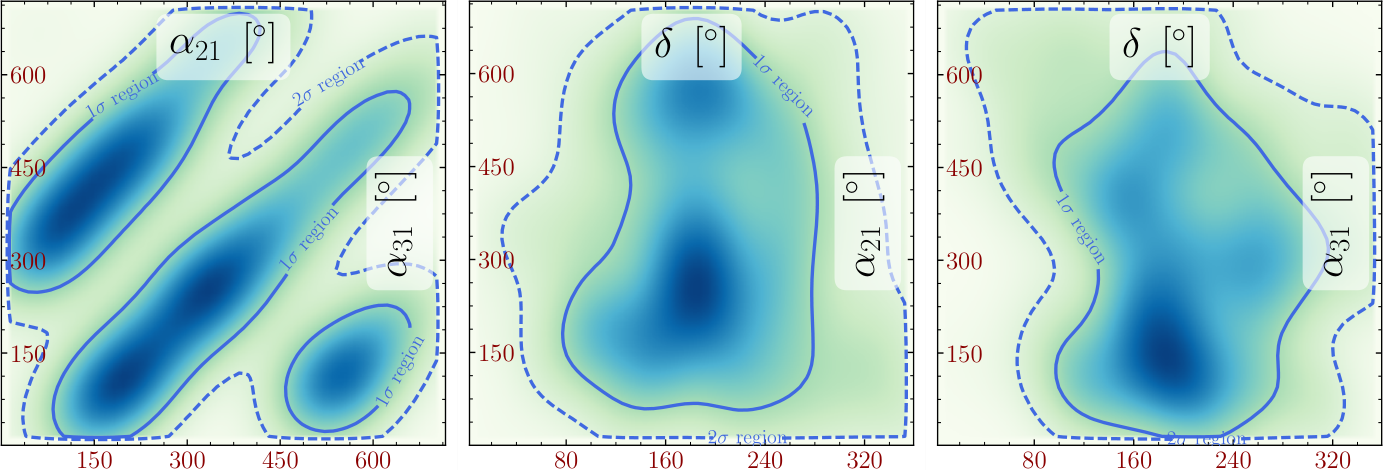
to define regions of and agreement with the observed value of the asymmetry. In addition we impose a bound on the sum of neutrino masses of which is consistent with the tritium beta-decay experiments [89, 90, 91] but more conservative than recent constraints from Planck [80]. In the numerical work of this section we allow only for the two lightest heavy Majorana neutrinos to decay (an excellent approximation) and we neglect lepton number-changing scattering processes, spectator effects [92, 20], thermal corrections [93, 94] and the inclusion of quantum statistical factors [95, 96, 97, 98] which typically introduces an error [27, 99, 100, 101]. To solve the density matrix equations we use the Python interface [102] to the LSODA algorithm [103] that is available in Scientific Python [104]. Due to the high-dimensionality of the parameter space we found the use of Multinest [105, 106, 107] (more explicitly, pyMultiNest [108], a wrapper around Multinest written in Python) particularly useful. In Fig. 8 we display the two-dimensional posterior probability plots for the -violating PMNS phases in the normal ordered and inverted ordered cases.
The results of this parameter search are shown in the form of two-dimensional projections in Fig. 19. For points in these regions of parameter space for which , the fine-tuning is which corresponds only to a very slight enhancement of the -matrix. The values of lightest neutrino mass for NO (IO) neutrino mass spectrum corresponding to this case are eV. For the best-fit values of the fitted parameters in the NO (IO) case we find: , , , GeV, GeV, . For the case of an NO light neutrino mass spectrum, we find that the observed baryon asymmetry may be obtained to within () with between (). For IO, the () range is (). Both of these scenarios comfortably incorporate the measured bounds on (Table 1). In what follows, we provide some explanation of these results and plots by introducing an analytical approximation which we use to study the scenarios where only the Dirac or only the Majorana phases provide violation.
3.2 Dependence of on the Dirac and Majorana Phases
| (∘) | (∘) | (∘) | ( | (∘) | (∘) | (∘) | (∘) | ||
In the scenario , it is appropriate to apply the two-flavour Boltzmann equations (Eq. (46)). These equations have the following analytical solution [109]
| (55) |
where it is assumed that the dominant contribution to the final asymmetry is from the lightest of the heavy Majorana neutrinos and that leptogenesis occurs in the strong washout regime. We denote the for which the washout becomes less than one as , , is the decay parameter for , and the for which leptogenesis is initiated as . As we are interested in those scenarios in which violation derives only from the phases of the PMNS matrix, we have the supplementary condition (or ) which we may use to simplify the solution to
| (56) |
with
| (57) |
At the benchmark point for normal ordering defined in Table 2, which we will use in the further analyses in the present section, we have:
| (58) | ||||
for violation from , and respectively. For the case in which provides the violation in Eq. (58), this phase gives a subdominant contribution to . As can be shown, is similarly weakly dependent on the phases. Thus, the phase dependence of the solutions of Eq. (56) does not come predominantly from the flavour factor but from the -asymmetry . However, in the case of providing the violation, the two terms of Eq. (58) are similar in magnitude and we may get a strong enhancement in . The final case where provides the violation is intermediate and should experience a slight phase-dependent enhancement from .
3.2.1 Dirac Phase Violation
In this subsection, we consider deviations from the benchmark point of Table 2 where we allow to vary but fix and . Given the pattern of -matrix angles, this ensures that any violation comes solely from . In this case, the -component of the -asymmetry is given by
| (59) |
Thus, given the approximate phase-independence of , we obtain a sinusoidal dependence of on , with when or . Keeping all other parameters fixed, we find that for GeV no value of can produce the observed baryon asymmetry of the Universe, the maximum value of as a function of is . We might scale the heavy Majorana neutrino masses by a constant value, as when the two-flavour approximation of Eq. (56) is valid, the factor scales in proportion with this constant and thus so does . In doing so, we find that the final asymmetry rises until GeV, where takes maximum value . After this, the simple scaling fails as one begins to enter the transition to what is usually the single-flavour regime.
Performing a detailed numerical parameter exploration we find that purely Dirac phase violation leads to successful leptogenesis for GeV, GeV and GeV. This is illustrated in Fig. 3 in which the plotted comes from solving the full density matrix equations. In this case, we have:
| (60) |
Given the different order of magnitude of the two terms in the expression for , the baryon asymmetry should exhibit dependence on only from and not from . Our theoretical expectations are borne out by the approximate sinusoidal dependence of on seen in Fig. 3.
3.2.2 Violation from the Majorana Phase
Here, we set but allow violation from . Setting all other parameters to their benchmark values we find
| (61) |
It follows from this expression for that at the -conserving values for we have (see also Fig. 4). This corresponds to the case of -conserving -matrix, -conserving PMNS matrix, but -violating interplay between the and PMNS matrix elements in leptogenesis [25]. In a similar way to the previous subsection, we find that no value of can achieve successful leptogenesis using this combination of phases and the benchmark values from Table 2. Thus, we find it necessary to scale all of the heavy Majorana neutrino masses by a common factor such that , may allow for successful leptogenesis. With this scaling we obtain the results plotted in Fig. 4. The deviation from pure (co)sinusoidal behaviour is explained by the -dependence of . For , varies relatively slowly exhibiting a global minimum at , resulting in a slightly modified sinusoidal dependence through this point in . A strong peak exists for around , which results in the peak of occurring before , as would be expected from the dependence of . The small sign-changing fluctuation around the zero at is a feature that does not appear in the solution of two-flavour Boltzmann equations and thus cannot be explained in terms of the analytic solution Eq. (56). However, the extra zeros of that are seen in Fig. 4 are due only to accidental cancellations and do not correspond to cases of -symmetry (unlike those at and ).
3.2.3 Violation from the Majorana Phase
We set and such that violation is provided by . Using the benchmark values for the other parameters from Table 2 we find:
| (62) |
Again we find that without scaling the heavy Majorana neutrino masses, no value of corresponds to successful leptogenesis. At we obtain the first point for which the observed baryon asymmetry is created and this is plotted in Fig. 5. We see that analytical expectation of a sinusoidal dependence of the baryon asymmetry () from Eq. (62) is present. exhibits a broad peak around which results in the slight shift to the centre of the otherwise sinusoidal peaks.
3.3 The Case of Decoupled
In this section, we review the case that the heaviest Majorana neutrino, , physically decouples. We restrict ourselves to normal ordered light neutrino masses. The resultant scenario with two relevant heavy Majorana neutrinos is the simplest (minimal) type I framework compatible with all neutrino data. In this scenario only two of the light neutrinos have non-zero masses since . For normal ordering, the -matrix may be parametrised as [110, 111, 112]
| (63) |
The resulting neutrino Yukawa matrix thus has , consistent with the premise that has decoupled. We choose to take in Eq. (63) to be real in order to have the condition of Eq. (16) satisfied. We assume further that at least one of the three phases in the PMNS matrix has a -violating value.
As with the previous sections, we have performed an exhaustive exploration of the parameter space where again we are primarily concerned with the situation in which violation is provided only by the PMNS phases. We choose to fix GeV and GeV such that the parameter space to explore is described by . In Fig. 6, we present the two-dimensional posterior projection for the case of normal ordering. Here, it is seen that with GeV, for normal ordering, successful leptogenesis may produce a baryon asymmetry with () agreement with the observed value for , ().
In Table 3, we provide a benchmark point for normal ordered leptogenesis, with purely low-energy violation and decoupled. At this point, the observed BAU is produced with a corresponding fine-tuning of . In Fig. 7, we illustrate a similar scenario, in which the violation is provided only by (, ), and where the observed baryon asymmetry is produced near . We conclude that, even for the minimal type I seesaw scenario with two heavy Majorana neutrinos exhibiting hierarchical mass spectrum, it is possible to generate the observed value of the baryon asymmetry with the requisite violation provided exclusively by the Dirac phase , and/or by the Majorana phase or .
Furthermore, we note that, in performing a similar investigation for the inverted ordering scenario, we find no point in the parameter space which corresponds to successful leptogenesis with decoupled in this mass window99 9 For IO light neutrino mass spectrum the decoupling of implies . In this case as well. with real -matrix. If, however, e.g., ( in the case of interest), we can have successful leptogenesis with the violation provided by the Dirac and/or Majorana phases in PMNS matrix also for the IO spectrum. These conclusions are in agreement with the results of [25] wherein one may find a detailed discussion of the cases considered in the present subsection.
| (∘) | (∘) | (∘) | ( | (∘) | |
Finally, in [25] the following necessary condition for successful leptogenesis in the case of NO spectrum with the requisite violation provided exclusively by the Dirac phase was obtained:
| (64) |
We recall that this condition was derived by using values of the the -conserving -matrix elements maximising the lepton asymmetry and assuming that the transition from two-flavour to one-flavour regime starts at GeV, i.e., that at GeV the two-flavour regime is fully effective.
4 Leptogenesis in the regime GeV
Successful thermal leptogenesis at intermediate scales may be accomplished through the combination of flavour effects and fine-tuned Yukawa matrices with [113, 78]. In Section 2.3, we first review these fine-tuned scenarios and then proceed to determine the subset among them in which the -matrix is -conserving while the PMNS matrix contains -violating phases. In Section 4.1 we present and analyse the results of a comprehensive search of the model parameter space for regions with successful leptogenesis compatible with these subsets where we have numerically solved the density matrix equations, for two-decaying heavy Majorana neutrinos, exactly. Following this, we consider in detail the scenarios in which violation is due solely to the Dirac phase in Section 4.2.1, or due only to the Majorana phases in Section 4.2.2 and Section 4.2.3. In Appendix B, we display results for GeV, where fine-tuning is also required.
We present an analytic approximation of the baryon asymmetry to find that the detailed dependence of the baryon asymmetry on the low energy phases may be roughly explained by the features of and . We reiterate that we apply these approximation simply to illustrate the qualitative behaviour of the solutions but we numerically solve the density matrix to produce all plots in this paper.
4.1 Results of Parameter Exploration


The options of Eq. (37) are satisfied by sixteen distinct -matrices which may be divided into four classes according to the corresponding parity vectors , (see Appendix A for definitions and further details). All such matrices are identical except for the placement of factors or . The phenomenological implications of each will be qualitatively similar except for the precise positions in parameter space that certain features occur. As we are primarily concerned with demonstrating the viability of leptogenesis with the fine-tuned Yukawa matrices (of the type in Eq. (28)) then we shall focus our numerical efforts on just one possible -matrix of the set of sixteen. Namely, we choose a scenario corresponding to , such that , .
For the numerical analysis, we follow the same procedure outlined in Section 3.1 with one additional constraint. At values of , higher-order corrections to the light neutrino mass become important. For this reason we fix and thereby avoid these problematic regions of the model parameter space.
In the parameter searches of this section, we consider two cases, in one we fix GeV (Fig. 8) and in the other we fix GeV (Fig. 9). We note that and and eV. 1010 10 In Appendix B, we demonstrate that one may lower as far as eV and still have successful leptogenesis in a albeit rather constrained parameter space. This allows for a comparison of the effects of two different degrees of fine-tuning, with the former corresponding usually to . This is close to the maximum fine-tuning (and correspondingly, the smallest non-resonant leptogenesis scale) for which second-order radiative corrections to the mass can be ignored [78].
For the scenario in which GeV, as anticipated, there is a large fine-tuning of . In the normal ordered case, we find that the observed baryon asymmetry may be obtained to within () with between (). For inverted ordering, the () range is (). With GeV, the fine-tuning is considerably less, at . In the normal ordered case, we find that the observed baryon asymmetry may be obtained to within () with between (). For inverted ordering, the () range is (). As in the previous section, we may explain these plots in detail by introducing an analytical approximation and the considering the simpler scenarios in which only the Dirac or only the Majorana phases provide violation. For brevity, we choose to perform this analysis only for GeV in the normal ordered scenario.
| (∘) | (∘) | (∘) | ( | (∘) | (∘) | (∘) | (∘) | ||
4.2 Dependence of on Dirac and Majorana Phases
In this section, we use the benchmark point given in Table 4, in order to analytically study leptogenesis from low-energy violation in the case that the lightest heavy Majorana neutrino has mass GeV, such that a relatively high degree of fine-tuning in the light neutrino masses is required. We choose this benchmark point as it allows us to accurately neglect the contributions from decays of the other heavy Majorana neutrinos and thus simplify the analysis.
With GeV, leptogenesis occurs in the three-flavour regime for which the three-flavoured Boltzmann equations are a good approximation to the density matrix equations and have approximate analytical solution [109]:
| (65) |
where we take into account the decays of only the lightest heavy Majorana neutrino. As we are most interested in the scenarios in which violation is due to PMNS phases only, i.e. , then we can re-express Eq. (65) as
| (66) |
where the asymmetry depends on the low-energy phases via and and from the difference of the inverse flavour projections:
| (67) |
However, for the case of Table 4, the two and three-flavour regime Boltzmann equations, to a high degree of accuracy give the same value of . Given the comparative simplicity of the two-flavour solution Eq. (56), we choose to use this for the practical purpose of simplifying the analysis.
For the benchmark parameter values listed in Table 4, we may find analytical approximations for the -asymmetries . Under the relatively good approximation, that 1111 11 The approximation is sufficiently precise as long as eV2., the asymmetry is given by
| (68) | ||||
Selecting and for , , such that and and is satisfied, we find the -asymmetry to be
| (69) | ||||
where, at our benchmark point, the coefficient of has magnitude approximately equal to . This form is particularly useful in order to isolate the dependence of the -asymmetry on the PMNS phases in the factor .
4.2.1 Dirac Phase Violation
We consider the possibility that the Majorana phases are -conserving: , (given the -matrix under consideration). The sole source of violation is and there is exact -invariance if . The corresponding is plotted in Fig. 10 alongside a parametric plot of against with parameter .1212 12 All plots involving in this work have been obtain by solving the full density matrix equations, allowing for the lightest pair of heavy Majorana neutrinos to decay and possibly (if indicated) include scattering effects.
From the -asymmetry, one expects to find proportional to
| (70) |
and thus sinusoidal in . However, the phase-dependent efficiency (flavour-factor) exhibits a sharp maximum around the region or . This modifies the sinusoidal dependence from the -asymmetries such that the extrema of are shifted towards the extreme values of , as in seen in Fig. 10. The small fluctuations around , are not captured by the Boltzmann equations (neither two-flavoured nor three-flavoured) and are only present when solving the full density matrix equations which take account of the finite size of the lepton thermal widths. The result is the addition of some accidental zeros in the variation which do not correspond to -conserving values of .
4.2.2 Violation from the Majorana Phase
Alternatively, consider the case of violation from , where , and all other parameters are set to their benchmark values of Table 4. The variation of with in this scenario is plotted on the left of Fig. 11. On the right of the same figure, we parametrically plot against with parameter . The baryon asymmetry vanishes at the -conserving values of and . However, as is seen in Fig. 11, at the -conserving values of , and since at these values the interplay between the -conserving and PMNS matrices leads to violation in leptogenesis [25].
The efficiency function , when plotted as a function of , exhibits a very strong narrow peak at and a much less pronounced peak at . As a consequence, the corresponding is modified from the simple cosine curve expected from the dependence of and on , which arises in the factors:
| (71) |
Thus, there is a sharp transition around . We can conclude then that the strong peak in is what has allowed the observed baryon asymmetry of the Universe to be reproduced. This peak originates in an accidental cancellation of terms in the function . There is no a priori reason to expect such a cancellation and it should be understood as a feature of the fine-tuned solutions that are being here studied. Thus, we see that the flavour-effects introduce a pair of accidental zeros of , one in the range and the other in .
4.2.3 Violation from the Majorana Phase
Finally, consider the case of violation from where , and for which the baryon asymmetry is plotted in the left plot of Fig. 12 and on the right we show the parametric dependence of the effective neutrino mass with against that of . The baryon asymmetry vanishes at the -conserving values of , and .
The efficiency function in this case is qualitatively similar to that for the case of : violation only strongly peaks at close to and to . Thus, we do not observe, in the left plot of Fig. 12, the simple dependence, as may be expected from the expression for ,
| (72) |
Rather, we find an enhanced positive peak near and an enhanced negative peak near .
4.2.4 Summary of Fine-Tuned Solutions with High Energy -Symmetry
The fine-tuned solutions we have discussed in this section share the property that they enhance through the production of a peak in the efficiency factor . In each projection coefficient,
| (73) |
the PMNS matrix cancels from the denominator such that all phase-dependence comes from that of in the numerator. In this subsection, we may safely use the usual Casas-Ibarra parametrisation (obtained by the replacement of with in Eq. (10)), to obtain
| (74) |
The absolute value is extremised when each term in the parentheses in Eq. (74) has a common complex phase or when terms may differ in complex phase by . This occurs at -conserving values of the PMNS phases and so the enhancement expected in the functions is likely to occur at -conserving phases also. As an example, around the benchmark point of Table 4, we find that with only contributing to violation (),
| (75) |
The absolute value of this function has extrema when or - the -conserving values. Moreover, the cancellation that occurs at is strong because of the similarity in magnitude of the two terms in Eq. (75). As a result of this there are strong peaks in which enhance .
This is a way in which the solutions are found to be fine-tuned as there is no reason to expect these two terms to be so similar in size. At these same points, the asymmetries are vanishing as is a symmetry in the leptonic sector. Thus , being proportional to the product of and , is strongly enhanced on either side of the -invariant points (for instance, around in the left plot of Fig. 11). Thus the fine-tuned solutions tend to achieve large of one-sign on one side of a -invariant point and large of the opposite sign on the other side. Similarly, this effect persists when all phases may contribute together to violation (Fig. 8 and Fig. 9). Thus, successful leptogenesis tends to occur near , when leptogenesis is achieved with fine-tuned light neutrino masses, as it is at intermediate scales ( GeV). Note that although we made these arguments based on the two-flavoured Boltzmann equations, very similar conclusions are reached based on considerations of and for the solutions of the three-flavoured Boltzmann equations. For this reason, one expects similar behaviour to hold even for lower values such as in Fig. 8.
Furthermore, one may usually argue that Dirac-phase leptogenesis suffers a suppression not present in Majorana phase leptogenesis due to the factors of that appear in the -asymmetries as shown in Eq. (70). However, for Dirac-phase leptogenesis , where the maximum absolute value of is , whereas for leptogenesis, with maximum absolute value . Thus, what is more relevant when leptogenesis occurs intermediate scales, is the degree of enhancement from that occurs due to fine-tuning.
Finally, as we observe in Fig. 9, the contours for , show a strong dependence on . A rough explanation of this is given by the dependence of on the Majorana phases. With fixed at its benchmark value, but and free to vary, this CP-asymmetry is given by
| (76) |
which exhibits a slightly dominant, -dependent contribution. This contribution is maximised when .
5 Leptogenesis in the regime GeV
In previous studies in which a connection between low-energy violation (-conserving ) and leptogenesis was established [26], the scale of leptogenesis was limited to . This allowed for the use of the two-flavour Boltzmann equations as shown in Eq. (46) where the -asymmetries and appear separately. The expectation had been that for , the single-flavour Boltzmann equation Eq. (41) would be appropriate. In this equation, the -asymmetries appear only in the factor and hence no baryon asymmetry may be produced. In Section 5.1 we argue that even at high scales , if is -conserving, then flavour effects are significant and that the density matrix equations do not reduce to the single flavour Boltzmann equations. Hence we conclude that viable leptogenesis may result from low energy violation. Finally, in Section 5.2 we proceed to numerically analyse this possibility in detail.
5.1 Flavour Effects with and High Energy -Symmetry

In Appendix C, we demonstrate that the complete formal solution of the density matrix equations (Eq. (49)), with one decaying heavy Majorana neutrino is
| (77) |
with
| (78) |
In a typical leptogenesis scenario, if , flavour effects are negligible and one obtains the well-known result:
| (79) |
which may be found by solving the single flavour Boltzmann equation. However, with a -conserving -matrix, such that violation is provided solely by the PMNS phases, one has and so the term in Eq. (77) becomes the dominant one:
| (80) |
If this is the case, then the baryon asymmetry is produced purely through flavour-effects from .
The physical effect of is that opposite asymmetries are produced in the and flavours due to the decay of : . However, with flavour effects, the lepton asymmetries and produced in the decay experience differing washouts such that and . It is an asymmetry produced by this method that is described in Eq. (80). The obvious question at this point is whether this can ever be large enough to produce the observed baryon asymmetry when .
| (∘) | (∘) | (∘) | ( | (∘) | (∘) | (∘) | ||
The density matrix equations may be conveniently expressed in terms of the vectors
| (81) | ||||
| (82) |
as
| (83) |
where
| (84) |
In terms of these quantities, the formal solution, with flavour effects neglected is:
| (85) |
Although flavour effects in high-scale leptogenesis may be negligible, this solution may not be accurately applied for finding in the case that . This is because there is a strong cancellation of components of the density matrix when computing , such that the errors made in neglecting flavour effects are dominant. For this reason, we make use of it only for finding the approximate behaviour of individual components of the density matrix and avoid applying it to situations where this cancellation occurs.
If the heavy Majorana neutrino masses are scaled by a common factor , such that , then: scales in proportion with , and do not scale with and varies inversely with . Consequently, according to Eq. (85), scales in proportion to , (with increasing precision for larger since we can better neglect the thermal widths). In the scaling of cancels that of and so does not scale with if . Thus, at sufficiently large values of , , given by Eq. (80), asymptotically approaches a non-zero constant. This is shown in Fig. 14 (d) over a range of values in which the ratios and are fixed. The curve increases ever more slowly for larger as the approximation leading to Eq. (85) becomes ever more precise. This may be interpreted as the transition region between the two flavour regime and the single flavour having grown infinitely large.1313 13 If, contrary to our scenario of interest, is -violating (), then the first term in parantheses of Eq. (77) eventually dominates the second for sufficiently large and the single flavour regime is entered. In each of the plots of Fig. 14, we see a dip in the density matrix solution curve near GeV. This feature is due to the difference in sign of the two-flavour solutions, for which , compared to that of the single flavour solutions, where (where these numbers are valid for plot (a) of Fig. 14 corresponding to -violating -matrix). The dip appears as a result of plotting the absolute value of on a logarithmic scale when passes through zero during the transition between these regimes.
In Appendix D, we discuss the robustness of the plateau that forms for large heavy Majorana neutrino masses when the effects of scattering and when a more realistic treatment of the right-handed taus are incorporated. In the next section we explore the parameter space of the three heavy Majorana neutrino type I seesaw with regard to the solutions of Eq. (108) with -conserving -matrix and .
5.2 Results of Parameter Exploration
At values of GeV, fine-tuning through large elements of the -matrix is not required for successful leptogenesis (if Majorana phases are allowed to play a role, otherwise large fine-tuning is required if only Dirac phases take effect). Thus, in this section we analyse the parameter space corresponding to real, and therefore -conserving, -matrices (), using the same numerical technique as described in Section 4.1. In order to perform this analysis we fix and again require in order to avoid the resonant regime. With a much higher value of , one would need a correspondingly a higher temperature of inflation. For this reason, we choose to illustrate the possibility of successful thermal leptogenesis at just one order of magnitude beyond the two-flavour to single-flavour transition temperature of GeV. In Fig. 13, we display the two-dimensional projection plots for both normal ordering and inverted ordering.
In the NO case, we find that the observed baryon asymmetry may be obtained to within () with between (). In the IO one, the () range is (). In what follows, we analyse these results by considering separately the cases of purely Dirac or purely Majorana violation. For brevity we consider only the case of NO spectrum.
5.3 Dependence of on the Dirac and Majorana Phases
As the final value of the baryon asymmetry becomes approximately constant for (see Fig. 14) with a -conserving -matrix, then one can can use the value of that is predicted by the two-flavour Boltzmann equations (2FBE) at the start of the transition as a proxy for the full solution of the density matrix equations (DME). That is,
| (86) |
provided that the ratios and are fixed. This has the advantage that we may again make use of the result in Eq. (56)
| (87) |
in order to gain an analytical understanding of the numerical solutions.
As in the analysis of Section 4.1, we investigate the cases where violation comes from precisely one of , or . Unlike the fine-tuned scenario previously considered, and consequently are approximately constant with the PMNS phases as would be expected from our discussion of the fine-tuned solutions in Section 4.2.4. Hence the phase-dependence of the can be understood by reference to alone. This may also be understood by reference to the Yukawa couplings when violation comes only from , or respectively:
| (88) | ||||
The difference in scale of the two terms means that the cancellation is never strong for any value of the phase and so the peaks in are not large. In this high scale case, is approximately constant and thus the plots of exhibit a nearly pure sinusoidal variation given by the -asymmetries below.
5.3.1 Dirac Phase violation
In this case, with a real , we have such that is the sole provider of all violation. The asymmetry is given by
| (89) |
in this scenario. Thus we obtain a sinusoidal dependence with when or . Fixing all other parameters at their benchmark value with , no value of can produce the observed baryon asymmetry of the Universe. Unlike in the case of intermediate scale leptogenesis, a small scaling of the heavy Majorana neutrino masses will not much increase the value of because of the plateau of Fig. 14. At the best-fit point of Table 5, with , allowing violation only from , the largest achieved is a factor smaller than the observed value. This is large enough that even enormously larger scales of the heavy masses cannot make -only leptogenesis a viable option.
An alternative for producing the observed baryon asymmetry of the Universe with violation only from is to work with an -matrix containing both zero and purely imaginary components which are -conserving and may potentially be large in magnitude. If for example, we choose such that all are either purely imaginary or zero, and take also, then by setting and , all violation will be due to . Varying and together in this setup, we find that is the smallest value for which the observed baryon asymmetry of the Universe is produced. With all other parameters equal to the values in Table 5, this corresponds to . Hence a noticeable degree of fine-tuning is required even at high scales to make the sole contributor to violation with viable leptogenesis. In Fig. 15, we plot the variation of with pure violation for this fine-tuned scenario in the left plot, and on the right we parametrically plot against as a function of .
5.3.2 Violation from the Majorana Phase
Similarly, when , the -asymmetry is
| (90) |
It follows from the preceding expression for that at the -conserving values of we have . This corresponds to the case of -conserving -matrix (), -conserving PMNS matrix, but -violating interplay between the and PMNS matrix elements in leptogenesis [25].
The corresponding , plotted in the left plot of Fig. 16 is thus a factor of higher and of opposite sign than in the previous case without fine-tuning. Thus, we obtain the observed baryon asymmetry of the Universe (or higher) for values of between about and . In the right plot of Fig. 16 is for the same scenario parametrically plotted against the effective neutrino mass with parameter .
5.3.3 Violation from the Majorana Phase
Finally, we turn to the scenario in which violation is provided entirely by , plotted on the left in of Fig. 17 for which
| (91) |
Similarly to the case discussed in the preceding subsection, we see that at the -conserving values of . This again corresponds to the case of violation in leptogenesis due to the interplay of the -conserving -matrix () and -conserving PMNS matrix [25].
Compared with the previous scenario, there is a sign flip and an enhancement by a factor of the resulting baryon asymmetry of the Universe. Thus, the observed BAU is achieved and exceeded for smaller values of , between about and . On the right of Fig. 17, we display a parametric plot for the same scenario with against the effective neutrino Majorana mass with the parameter .
6 Conclusions
In this paper we have investigated the connection between leptogenesis and low energy leptonic violation over a large range of scales . We summarise our main findings below:
- •
Firstly, we revisited the question of the possibility of successful thermal leptogenesis at scales . At such scales, tau-Yukawa interactions are in equilibrium, such that there are sufficiently frequent interactions between the leptons and the early Universe plasma causing decoherence between the tau flavour from the other flavour components. We show that successful leptogenesis is indeed possible in this range of scales in the case that the PMNS phases provide all of the violation in the model. By performing parameter explorations at GeV and GeV, we found that some degree of fine-tuning, , is required for these particular mass scales (with the degree of fine-tuning diminishing as one goes to higher values of ).
- •
By demanding pure Dirac phase or pure Majorana phase violation, we found that each phase alone can produce the correct -asymmetry, with the cases of Majorana phases requiring, in general, a somewhat lower value of than those required for the Dirac phase.
- •
If leptogenesis takes place at scales GeV, then all three of the leptonic flavour components involved in leptogenesis will decohere. For masses in this range ( GeV and GeV), we determined the regions of parameter space in which low energy leptonic violation, provided by either the Dirac or the Majorana phases individually, leads to successful intermediate scale leptogenesis. At these scales a large amount of fine-tuning () is required between the tree-level and one-loop neutrino masses. We restricted ourselves to fine-tuning such that and in doing so have found an approximate lower bound of (consistent with the conclusions of [78]).
- •
We studied the possibility of pure Dirac phase violation and showed that for , in order to produce the observed baryon asymmetry. Similarly for the purely Majorana phase violation and again , for , we obtain a bound whereas for we obtained . Observables depending on the Dirac and Majorana phases, for example or , may be well within experimental bounds in the same parts of parameter space in which leptogenesis is successful. The Dirac phase is only very weakly constrained, with the tightest constraint being , for agreement with the observed BAU, which comes from assuming normal ordering and GeV.
- •
If leptogenesis takes place at high scales, with GeV, interactions between the leptons and the early Universe plasma only very weakly decohere the tau flavour from the other flavour components. Normally, this leads to the conclusion that the single flavour Boltzmann equations are an appropriate description of the process. However, we have demonstrated that, if violation arises only in the low energy leptonic sector, the effects of decoherence cannot be neglected. Therefore, one should not ignore the phenomenology of high-scale leptogenesis with purely low-energy violation.
- •
We explored the parameter space at GeV, finding regions in which thermal leptogenesis is a viable explanation of the BAU. We found that the strongest constraint on is for normal ordering, for which we require to produce a baryon asymmetry within of the observed value. With only Dirac phase violation, we have concluded that it is not possible produce the observed baryon asymmetry of the Universe unless one introduces significant fine-tuning in the light neutrino masses. We argued that there is no scale of the heavy Majorana neutrino masses beyond for which Dirac phase leptogenesis may be made to work without this fine-tuning. However, with pure Majorana phase violation, we found that successful leptogenesis is possible with essentially no fine-tuning.
The results of this article underscore the significance of understanding leptonic violation through experimental searches for Dirac and/or Majorana leptonic violation. We have departed from previous literature by concluding that low energy leptonic -violating phases may always be relevant to the production of the baryon asymmetry in the leptogenesis scenario. It has commonly been thought that their relevance was limited to the window of masses . However, we have shown this window to be significantly wider: Dirac and Majorana phases may be crucial to leptogenesis even at scales as low as , or as high as .
Acknowledgements.
We would like to thank Pasquale Di Bari for helpful conversations regarding the density matrix equations. K.M. and S.P. acknowledge the (partial) support from the European Research Council under the European Union Seventh Framework Programme (FP/2007-2013) / ERC Grant NuMass agreement n. [617143]. S.P. would like to acknowledge partial support from the Wolfson Foundation and the Royal Society, and also thanks SISSA for support and hospitality during part of this work. S.P. and S.T.P. acknowledge partial support from the European Unions Horizon 2020 research and innovation programme under the Marie Sklodowska Curie grant agreements No 690575 (RISE InvisiblesPlus) and No 674896 (ITN ELUSIVE). The work of S.T.P. was supported in part by the INFN program on Theoretical Astroparticle Physics (TASP) and by the World Premier International Research Center Initiative (WPI Initiative), MEXT, Japan. This manuscript has been authored by Fermi Research Alliance, LLC under Contract No. DE-AC02-07CH11359 with the U.S. Department of Energy, Office of Science, Office of High Energy Physics. J.T. would like to express a special thanks to the Mainz Institute for Theoretical Physics (MITP) and International School for Advanced Studies (SISSA) for their hospitality and support where part of this work was completed.Appendix A Classes of -Conserving -matrix
With the parameters , and left arbitrary, there are possible -matrices which lead to the fine-tuned light neutrino masses required for successful leptogenesis (Eq. (27)). For any of these matrices, the absolute values of the elements are equal, with the elements themselves differing only by factors or . When there is an exact -symmetry, then each -matrix satisfies the condition in Eq. (16). This allows for a scheme of classification according the phases , they correspond to. In this section we present a single example of a matrix for each class1414 14 Here we neglect terms involving factors or such that, as given, these matrices are not strictly orthogonal.:
, and and :
in which the second form results from the neglect of terms involving factors and . , and and :
, and and :
, and and :
Appendix B Further results
In Fig. 18 we demonstrate the possibility of fine-tuned leptogenesis in the case of normal ordering with GeV and eV. This is a variant of the case considered in the main body for which the light neutrino masses are significantly reduced below all present cosmological or current generation direct bounds. We note that lowering the light neutrino masses in this way severely constrains the viable parameter space over that in Fig. 8 such that , and . Typical fine-tuning in the viable regions is .
In the cases of and eV with GeV, and we did not find a region in the relevant parameter space in which one could have successful leptogenesis.


In Fig. 19 we present results for GeV. We find that a fine-tuning of the light neutrino masses at the best-fit points. In the normal ordered case, we find that the observed baryon asymmetry may be obtained to within () with between (). While for inverted ordering, the () range is (). This is significantly higher than the case for which GeV where the fine-tuning is considerably less at . In the normal ordered case, we find that the observed baryon asymmetry may be obtained to within () with between (). For inverted ordering, the () range is ().
Appendix C Single Flavour Boltzmann Equations from Density Matrix Equations
In this appendix we find the conditions under which the density matrix equations (Eq. (49)) approximate to the single flavour Boltzmann equations. We begin by analysing the criteria under which the single flavour Boltzmann equation
| (92) |
emerges as an approximation from the density matrix equations, which, written in the (, )-basis are
| (93) | ||||
As , we find an equation for the evolution of by adding the second and third equations together, obtaining
| (94) |
If this were to reproduce the single flavour limit, then we should find that the coefficient of :
| (95) |
is equal to in the limit that is small. Recalling that , then one should expect, that in the limit of small thermal widths,
| (96) |
In order to demonstrate this equality, first we show that the -derivative of equals the -derivative of meaning that the quantities themselves may differ only by a constant. Then we note that, since at the quantities are equal, then they must be equal for all .
By multiplication of the relevant equations in Eq. (93), we obtain the -evolution of :
| (97) | ||||
By similar means we obtain the -evolution of :
Neglecting , as we expect this to be small in the single-flavour regime, then we need only show that
| (98) |
and then it is demonstrated that the coefficient of in Eq. (94) is approximately equal to and thus the single flavour equations are recovered.
The relation of Eq. (98) can be put into a more suggestive form if we use to re-express it thus
| (99) |
The right-hand side of this equation is merely the trace of the -asymmetry tensor in the -basis. Thus, we suspect that the left-hand side is merely the trace expressed in an unfamiliar basis. This can be confirmed to be the case by construction of the unitary matrix
| (100) |
then, by explicit calculation it can be seen that the left-hand side is the result of summing the diagonals (evaluating the trace in a particular basis) of
| (101) |
Thus, we may conclude that, if we set , we are left with
| (102) |
and so
| (103) |
Since at the initial , then we may conclude that, if , then
| (104) |
which is the single-flavour limit.
If we don’t set , then we have
| (105) |
which suggests that we should write the integro-differential equation
| (106) |
We define
| (107) |
for brevity, then using the integrating factor method, arrive at a solution
For large , the thermal width is very small and so the term in is usually neglected in comparison with the first.
Appendix D Robustness of the High-Scale Plateau
In the transition region, the approximation that left-handed leptons are produced and destroyed at the same rate by flavour effects is somewhat inaccurate. In fact we should consider a slightly more accurate version of the density matrix equations in which the asymmetry density of right-handed leptons, is computed. Then, the density matrix equations are
| (108) | ||||
The simpler set we previously considered result from the assumption that is large enough to enforce . Clearly this is inaccurate for the situation under consideration where . We should now append to an extra term such that
| (109) |
Now in this solution, there is a term in which scales approximately as and a term in which, it may be shown and thus exhibits a approximate invariance under a scaling as does .
It may be added that scattering effects can be incorporated by modifying the decay function and the washout [11]. The new decay function which depends on a scattering part is still multiplied by zero in the case and is thus unimportant. The new washout function is multiplied by which depends on through . Thus, the plateau demonstrated in Fig. 14 picks up some unimportant logarithmic dependence on in addition to the small variation when scattering is neglected. In the numerical calculations of Section 5, the effects of scattering are included.
References
- (1) A. D. Sakharov, Violation of CP Invariance, c Asymmetry, and Baryon Asymmetry of the Universe, Pisma Zh. Eksp. Teor. Fiz. 5 (1967) 32–35.
- (2) Super-Kamiokande collaboration, Y. Fukuda et al., Evidence for oscillation of atmospheric neutrinos, Phys. Rev. Lett. 81 (1998) 1562–1567, [hep-ex/9807003].
- (3) V. A. Kuzmin, V. A. Rubakov and M. E. Shaposhnikov, On the Anomalous Electroweak Baryon Number Nonconservation in the Early Universe, Phys. Lett. 155B (1985) 36.
- (4) S. Yu. Khlebnikov and M. E. Shaposhnikov, The Statistical Theory of Anomalous Fermion Number Nonconservation, Nucl. Phys. B308 (1988) 885–912.
- (5) P. Minkowski, at a Rate of One Out of Muon Decays?, Phys. Lett. B67 (1977) 421–428.
- (6) T. Yanagida, HORIZONTAL SYMMETRY AND MASSES OF NEUTRINOS, Conf. Proc. C7902131 (1979) 95–99.
- (7) M. Gell-Mann, P. Ramond and R. Slansky, Complex Spinors and Unified Theories, Conf. Proc. C790927 (1979) 315–321, [1306.4669].
- (8) R. N. Mohapatra and G. Senjanovic, Neutrino Mass and Spontaneous Parity Violation, Phys. Rev. Lett. 44 (1980) 912.
- (9) M. Fukugita and T. Yanagida, Baryogenesis Without Grand Unification, Phys. Lett. B174 (1986) 45–47.
- (10) W. Buchmuller and M. Plumacher, Baryon asymmetry and neutrino mixing, Phys. Lett. B389 (1996) 73–77, [hep-ph/9608308].
- (11) W. Buchmuller, P. Di Bari and M. Plumacher, Leptogenesis for pedestrians, Annals Phys. 315 (2005) 305–351, [hep-ph/0401240].
- (12) W. Buchmuller, R. D. Peccei and T. Yanagida, Leptogenesis as the origin of matter, Ann. Rev. Nucl. Part. Sci. 55 (2005) 311–355, [hep-ph/0502169].
- (13) A. Pilaftsis, CP violation and baryogenesis due to heavy Majorana neutrinos, Phys. Rev. D56 (1997) 5431–5451, [hep-ph/9707235].
- (14) K. Nakamura and S. Petcov, (Particle Data Group), Phys. Rev. D98 (2018) 030001.
- (15) G. C. Branco, T. Morozumi, B. M. Nobre and M. N. Rebelo, A Bridge between CP violation at low-energies and leptogenesis, Nucl. Phys. B617 (2001) 475–492, [hep-ph/0107164].
- (16) G. C. Branco, R. Gonzalez Felipe, F. R. Joaquim, I. Masina, M. N. Rebelo and C. A. Savoy, Minimal scenarios for leptogenesis and CP violation, Phys. Rev. D67 (2003) 073025, [hep-ph/0211001].
- (17) T. Endoh, S. Kaneko, S. K. Kang, T. Morozumi and M. Tanimoto, CP violation in neutrino oscillation and leptogenesis, Phys. Rev. Lett. 89 (2002) 231601, [hep-ph/0209020].
- (18) P. H. Frampton, S. L. Glashow and T. Yanagida, Cosmological sign of neutrino CP violation, Phys. Lett. B548 (2002) 119–121, [hep-ph/0208157].
- (19) Y. Shimizu, K. Takagi and M. Tanimoto, Neutrino CP violation and sign of baryon asymmetry in the minimal seesaw model, Phys. Lett. B778 (2018) 6–16, [1711.03863].
- (20) E. Nardi, Y. Nir, J. Racker and E. Roulet, On Higgs and sphaleron effects during the leptogenesis era, JHEP 01 (2006) 068, [hep-ph/0512052].
- (21) A. Abada, S. Davidson, A. Ibarra, F. X. Josse-Michaux, M. Losada and A. Riotto, Flavour Matters in Leptogenesis, JHEP 09 (2006) 010, [hep-ph/0605281].
- (22) A. Abada, S. Davidson, F.-X. Josse-Michaux, M. Losada and A. Riotto, Flavor issues in leptogenesis, JCAP 0604 (2006) 004, [hep-ph/0601083].
- (23) R. Barbieri, P. Creminelli, A. Strumia and N. Tetradis, Baryogenesis through leptogenesis, Nucl. Phys. B575 (2000) 61–77, [hep-ph/9911315].
- (24) H. B. Nielsen and Y. Takanishi, Baryogenesis via lepton number violation and family replicated gauge group, Nucl. Phys. B636 (2002) 305–337, [hep-ph/0204027].
- (25) S. Pascoli, S. T. Petcov and A. Riotto, Connecting low energy leptonic CP-violation to leptogenesis, Phys. Rev. D75 (2007) 083511, [hep-ph/0609125].
- (26) S. Pascoli, S. T. Petcov and A. Riotto, Leptogenesis and Low Energy CP Violation in Neutrino Physics, Nucl. Phys. B774 (2007) 1–52, [hep-ph/0611338].
- (27) S. Blanchet and P. Di Bari, Flavor effects on leptogenesis predictions, JCAP 0703 (2007) 018, [hep-ph/0607330].
- (28) G. C. Branco, R. Gonzalez Felipe and F. R. Joaquim, A New bridge between leptonic CP violation and leptogenesis, Phys. Lett. B645 (2007) 432–436, [hep-ph/0609297].
- (29) A. Anisimov, S. Blanchet and P. Di Bari, Viability of Dirac phase leptogenesis, JCAP 0804 (2008) 033, [0707.3024].
- (30) E. Molinaro and S. T. Petcov, The Interplay Between the ’Low’ and ’High’ Energy CP-Violation in Leptogenesis, Eur. Phys. J. C61 (2009) 93–109, [0803.4120].
- (31) E. Molinaro and S. T. Petcov, A Case of Subdominant/Suppressed ’High Energy’ Contribution to the Baryon Asymmetry of the Universe in Flavoured Leptogenesis, Phys. Lett. B671 (2009) 60–65, [0808.3534].
- (32) M. J. Dolan, T. P. Dutka and R. R. Volkas, Dirac-Phase Thermal Leptogenesis in the extended Type-I Seesaw Model, JCAP 1806 (2018) 012, [1802.08373].
- (33) C. Hagedorn, R. N. Mohapatra, E. Molinaro, C. C. Nishi and S. T. Petcov, CP Violation in the Lepton Sector and Implications for Leptogenesis, 1711.02866.
- (34) G. C. Branco, A. J. Buras, S. Jager, S. Uhlig and A. Weiler, Another look at minimal lepton flavour violation, , leptogenesis, and the ratio , JHEP 09 (2007) 004, [hep-ph/0609067].
- (35) L. Merlo and S. Rosauro-Alcaraz, Predictive Leptogenesis from Minimal Lepton Flavour Violation, JHEP 07 (2018) 036, [1801.03937].
- (36) C. C. Nishi, B. L. Sánchez-Vega and G. Souza Silva, reflection symmetry with a high scale texture-zero, 1806.07412.
- (37) A. Meroni, E. Molinaro and S. T. Petcov, Revisiting Leptogenesis in a SUSY SU(5) x T’ Model of Flavour, Phys. Lett. B710 (2012) 435–445, [1203.4435].
- (38) R. N. Mohapatra and C. C. Nishi, Implications of flavored CP symmetry of leptons, JHEP 08 (2015) 092, [1506.06788].
- (39) C. Hagedorn and E. Molinaro, Flavor and CP symmetries for leptogenesis and decay, Nucl. Phys. B919 (2017) 404–469, [1602.04206].
- (40) P. Chen, G.-J. Ding and S. F. King, Leptogenesis and residual CP symmetry, JHEP 03 (2016) 206, [1602.03873].
- (41) C.-C. Li and G.-J. Ding, Implications of residual CP symmetry for leptogenesis in a model with two right-handed neutrinos, Phys. Rev. D96 (2017) 075005, [1701.08508].
- (42) L. Covi, J. E. Kim, B. Kyae and S. Nam, Leptogenesis with high-scale electroweak symmetry breaking and an extended Higgs sector, Phys. Rev. D94 (2016) 065004, [1601.00411].
- (43) S. M. Bilenky, J. Hosek and S. T. Petcov, On Oscillations of Neutrinos with Dirac and Majorana Masses, Phys. Lett. 94B (1980) 495–498.
- (44) I. Esteban, M. C. Gonzalez-Garcia, M. Maltoni, I. Martinez-Soler and T. Schwetz, Updated fit to three neutrino mixing: exploring the accelerator-reactor complementarity, JHEP 01 (2017) 087, [1611.01514].
- (45) A. Pilaftsis, Radiatively induced neutrino masses and large Higgs neutrino couplings in the standard model with Majorana fields, Z. Phys. C55 (1992) 275–282, [hep-ph/9901206].
- (46) D. Aristizabal Sierra and C. E. Yaguna, On the importance of the 1-loop finite corrections to seesaw neutrino masses, JHEP 08 (2011) 013, [1106.3587].
- (47) J. Lopez-Pavon, S. Pascoli and C.-f. Wong, Can heavy neutrinos dominate neutrinoless double beta decay?, Phys. Rev. D87 (2013) 093007, [1209.5342].
- (48) W. Grimus and L. Lavoura, One-loop corrections to the seesaw mechanism in the multi-Higgs-doublet standard model, Phys. Lett. B546 (2002) 86–95, [hep-ph/0207229].
- (49) J. A. Casas and A. Ibarra, Oscillating neutrinos and muon —> e, gamma, Nucl. Phys. B618 (2001) 171–204, [hep-ph/0103065].
- (50) J. Lopez-Pavon, E. Molinaro and S. T. Petcov, Radiative Corrections to Light Neutrino Masses in Low Scale Type I Seesaw Scenarios and Neutrinoless Double Beta Decay, JHEP 11 (2015) 030, [1506.05296].
- (51) S. M. Bilenky and S. T. Petcov, Massive Neutrinos and Neutrino Oscillations, Rev. Mod. Phys. 59 (1987) 671.
- (52) T2K collaboration, K. Abe et al., The T2K Experiment, Nucl. Instrum. Meth. A659 (2011) 106–135, [1106.1238].
- (53) NOvA collaboration, D. S. Ayres et al., NOvA: Proposal to Build a 30 Kiloton Off-Axis Detector to Study Oscillations in the NuMI Beamline, n/a (2004) , [hep-ex/0503053].
- (54) Daya Bay collaboration, F. P. An et al., Observation of electron-antineutrino disappearance at Daya Bay, Phys. Rev. Lett. 108 (2012) 171803, [1203.1669].
- (55) RENO collaboration, J. K. Ahn et al., Observation of Reactor Electron Antineutrino Disappearance in the RENO Experiment, Phys. Rev. Lett. 108 (2012) 191802, [1204.0626].
- (56) Double Chooz collaboration, F. Ardellier et al., Double Chooz: A Search for the neutrino mixing angle theta(13), n/a (2006) , [hep-ex/0606025].
- (57) N. Cabibbo, Time reversal violation in neutrino oscillation, Physics Letters B 72 (1978) 333 – 335.
- (58) S. Bilenky, J. Hošek and S. Petcov, On the oscillations of neutrinos with dirac and majorana masses, Physics Letters B 94 (1980) 495 – 498.
- (59) V. D. Barger, K. Whisnant and R. J. N. Phillips, CP Violation in Three Neutrino Oscillations, Phys. Rev. Lett. 45 (1980) 2084.
- (60) P. I. Krastev and S. T. Petcov, Resonance Amplification and t Violation Effects in Three Neutrino Oscillations in the Earth, Phys. Lett. B205 (1988) 84–92.
- (61) DUNE collaboration, R. Acciarri et al., Long-Baseline Neutrino Facility (LBNF) and Deep Underground Neutrino Experiment (DUNE), 1512.06148.
- (62) Hyper-Kamiokande Proto-Collaboration collaboration, K. Abe et al., Physics potential of a long-baseline neutrino oscillation experiment using a J-PARC neutrino beam and Hyper-Kamiokande, PTEP 2015 (2015) 053C02, [1502.05199].
- (63) S. M. Bilenky, S. Pascoli and S. T. Petcov, Majorana neutrinos, neutrino mass spectrum, CP violation and neutrinoless double beta decay. 1. The Three neutrino mixing case, Phys. Rev. D64 (2001) 053010, [hep-ph/0102265].
- (64) S. Pascoli, S. T. Petcov and L. Wolfenstein, Searching for the CP violation associated with Majorana neutrinos, Phys. Lett. B524 (2002) 319–331, [hep-ph/0110287].
- (65) S. Pascoli, S. T. Petcov and T. Schwetz, The Absolute neutrino mass scale, neutrino mass spectrum, majorana CP-violation and neutrinoless double-beta decay, Nucl. Phys. B734 (2006) 24–49, [hep-ph/0505226].
- (66) V. Barger, S. L. Glashow, P. Langacker and D. Marfatia, No go for detecting CP violation via neutrinoless double beta decay, Phys. Lett. B540 (2002) 247–251, [hep-ph/0205290].
- (67) S. Pascoli and S. T. Petcov, The SNO solar neutrino data, neutrinoless double beta decay and neutrino mass spectrum, Phys. Lett. B544 (2002) 239–250, [hep-ph/0205022].
- (68) M. Blennow, E. Fernandez-Martinez, J. Lopez-Pavon and J. Menendez, Neutrinoless double beta decay in seesaw models, JHEP 07 (2010) 096, [1005.3240].
- (69) J. D. Vergados, H. Ejiri and F. Šimkovic, Neutrinoless double beta decay and neutrino mass, Int. J. Mod. Phys. E25 (2016) 1630007, [1612.02924].
- (70) M. Doi, T. Kotani, H. Nishiura, K. Okuda and E. Takasugi, Cp violation in majorana neutrinos, Physics Letters B 102 (1981) 323 – 326.
- (71) L. Wolfenstein, CP Properties of Majorana Neutrinos and Double beta Decay, Phys. Lett. 107B (1981) 77–79.
- (72) S. M. Bilenky, N. P. Nedelcheva and S. T. Petcov, Some Implications of the CP Invariance for Mixing of Majorana Neutrinos, Nucl. Phys. B247 (1984) 61–69.
- (73) B. Kayser, CPT, CP, and c Phases and their Effects in Majorana Particle Processes, Phys. Rev. D30 (1984) 1023.
- (74) KamLAND-Zen collaboration, A. Gando et al., Search for Majorana Neutrinos near the Inverted Mass Hierarchy Region with KamLAND-Zen, Phys. Rev. Lett. 117 (2016) 082503, [1605.02889].
- (75) S. Dell’Oro, S. Marcocci, M. Viel and F. Vissani, Neutrinoless double beta decay: 2015 review, Adv. High Energy Phys. 2016 (2016) 2162659, [1601.07512].
- (76) S. Blanchet and P. Di Bari, New aspects of leptogenesis bounds, Nucl. Phys. B807 (2009) 155–187, [0807.0743].
- (77) S. Antusch, S. Blanchet, M. Blennow and E. Fernandez-Martinez, Non-unitary Leptonic Mixing and Leptogenesis, JHEP 01 (2010) 017, [0910.5957].
- (78) K. Moffat, S. Pascoli, S. T. Petcov, H. Schulz and J. Turner, Three-Flavoured Non-Resonant Leptogenesis at Intermediate Scales, 1804.05066.
- (79) Particle Data Group collaboration, C. Patrignani et al., Review of Particle Physics, Chin. Phys. C40 (2016) 100001.
- (80) Planck collaboration, P. A. R. Ade et al., Planck 2015 results. XIII. Cosmological parameters, Astron. Astrophys. 594 (2016) A13, [1502.01589].
- (81) A. De Simone and A. Riotto, On the impact of flavour oscillations in leptogenesis, JCAP 0702 (2007) 005, [hep-ph/0611357].
- (82) S. Blanchet, P. Di Bari and G. G. Raffelt, Quantum Zeno effect and the impact of flavor in leptogenesis, JCAP 0703 (2007) 012, [hep-ph/0611337].
- (83) S. Blanchet, P. Di Bari, D. A. Jones and L. Marzola, Leptogenesis with heavy neutrino flavours: from density matrix to Boltzmann equations, JCAP 1301 (2013) 041, [1112.4528].
- (84) L. Covi, E. Roulet and F. Vissani, CP violating decays in leptogenesis scenarios, Phys. Lett. B384 (1996) 169–174, [hep-ph/9605319].
- (85) A. Fowlie and M. H. Bardsley, Superplot: a graphical interface for plotting and analysing MultiNest output, Eur. Phys. J. Plus 131 (2016) 391, [1603.00555].
- (86) A. Pilaftsis and T. E. J. Underwood, Resonant leptogenesis, Nucl. Phys. B692 (2004) 303–345, [hep-ph/0309342].
- (87) L. Covi and E. Roulet, Baryogenesis from mixed particle decays, Phys. Lett. B399 (1997) 113–118, [hep-ph/9611425].
- (88) W. Buchmuller and M. Plumacher, CP asymmetry in Majorana neutrino decays, Phys. Lett. B431 (1998) 354–362, [hep-ph/9710460].
- (89) C. Weinheimer, Direct neutrino mass experiments: Present and future, Nucl. Phys. Proc. Suppl. 118 (2003) 279–286.
- (90) C. Kraus et al., Final results from phase II of the Mainz neutrino mass search in tritium beta decay, Eur. Phys. J. C40 (2005) 447–468, [hep-ex/0412056].
- (91) V. M. Lobashev et al., Direct search for neutrino mass and anomaly in the tritium beta-spectrum: Status of ’Troitsk neutrino mass’ experiment, Nucl. Phys. Proc. Suppl. 91 (2001) 280–286.
- (92) W. Buchmuller and M. Plumacher, Spectator processes and baryogenesis, Phys. Lett. B511 (2001) 74–76, [hep-ph/0104189].
- (93) C. P. Kiessig, M. Plumacher and M. H. Thoma, Decay of a Yukawa fermion at finite temperature and applications to leptogenesis, Phys. Rev. D82 (2010) 036007, [1003.3016].
- (94) G. F. Giudice, A. Notari, M. Raidal, A. Riotto and A. Strumia, Towards a complete theory of thermal leptogenesis in the SM and MSSM, Nucl. Phys. B685 (2004) 89–149, [hep-ph/0310123].
- (95) A. De Simone and A. Riotto, Quantum Boltzmann Equations and Leptogenesis, JCAP 0708 (2007) 002, [hep-ph/0703175].
- (96) M. Beneke, B. Garbrecht, C. Fidler, M. Herranen and P. Schwaller, Flavoured Leptogenesis in the CTP Formalism, Nucl. Phys. B843 (2011) 177–212, [1007.4783].
- (97) A. Anisimov, W. Buchmüller, M. Drewes and S. Mendizabal, Quantum Leptogenesis I, Annals Phys. 326 (2011) 1998–2038, [1012.5821].
- (98) M. Beneke, B. Garbrech, M. Herranen and P. SchwallerNucl. Phys. B838 (2010) 1–27, [1002.1326].
- (99) T. Frossard, A. Kartavtsev and D. Mitrouskas, Systematic approach to L=1 processes in thermal leptogenesis, Phys. Rev. D87 (2013) 125006, [1304.1719].
- (100) E. Nardi, J. Racker and E. Roulet, CP violation in scatterings, three body processes and the Boltzmann equations for leptogenesis, JHEP 09 (2007) 090, [0707.0378].
- (101) B. Garbrecht and P. Schwaller, Spectator Effects during Leptogenesis in the Strong Washout Regime, JCAP 1410 (2014) 012, [1404.2915].
- (102) W. Weckesser, odeintw: Complex and matrix differential equations., 2014–.
- (103) “A. C. Hindmarsh, “ODEPACK, A Systematized Collection of ODE Solvers,” in Scientific Computing, R. S. Stepleman et al. (eds.), North-Holland, Amsterdam, 1983 (vol. 1 of IMACS Transactions on Scientific Computation), pp. 55-64..”
- (104) E. Jones, T. Oliphant, P. Peterson et al., SciPy: Open source scientific tools for Python, 2001–.
- (105) F. Feroz, M. P. Hobson and M. Bridges, MultiNest: an efficient and robust Bayesian inference tool for cosmology and particle physics, Mon. Not. Roy. Astron. Soc. 398 (2009) 1601–1614, [0809.3437].
- (106) F. Feroz and M. P. Hobson, Multimodal nested sampling: an efficient and robust alternative to MCMC methods for astronomical data analysis, Mon. Not. Roy. Astron. Soc. 384 (2008) 449, [0704.3704].
- (107) F. Feroz, M. P. Hobson, E. Cameron and A. N. Pettitt, Importance Nested Sampling and the MultiNest Algorithm, ArXiv e-prints (June, 2013) , [1306.2144].
- (108) Buchner, J., Georgakakis, A., Nandra, K., Hsu, L., Rangel, C., Brightman, M. et al., X-ray spectral modelling of the agn obscuring region in the cdfs: Bayesian model selection and catalogue, A&A 564 (2014) A125.
- (109) C. S. Fong, E. Nardi and A. Riotto, Leptogenesis in the Universe, Adv. High Energy Phys. 2012 (2012) 158303, [1301.3062].
- (110) A. Ibarra and G. G. Ross, Neutrino phenomenology: The Case of two right-handed neutrinos, Phys. Lett. B591 (2004) 285–296, [hep-ph/0312138].
- (111) S. Antusch, P. Di Bari, D. A. Jones and S. F. King, Leptogenesis in the Two Right-Handed Neutrino Model Revisited, Phys. Rev. D86 (2012) 023516, [1107.6002].
- (112) S. Blanchet, Dirac phase leptogenesis, J. Phys. Conf. Ser. 120 (2008) 022007, [0710.0570].
- (113) S. Lavignac, I. Masina and C. A. Savoy, Large solar angle and seesaw mechanism: A Bottom up perspective, Nucl. Phys. B633 (2002) 139–170, [hep-ph/0202086].