Estimating the Frequency Coupling Matrix from Network Measurements
Abstract
Power converters are present in increasing numbers in the electric power grid. They are a major source of harmonic currents and voltages, which can reduce power quality and trip protection devices. The frequency coupling matrix (FCM) is a general technique for modeling converter harmonics. It can be obtained through experimental characterization or, given a converter’s internal parameters, direct calculation. In this paper, we estimate FCMs from network measurements. We give a novel harmonic reduction theorem for computing equivalent, virtual FCMs for unobservable portions of a network. We estimate FCMs and harmonic line admittances from PMU measurements, and give an efficient online version for the FCM problem. We test our approaches on a numerical example, and show that the estimation error is low under noisy observations.
Index Terms:
estimation, frequency coupling matrix, harmonics, power systemsI Introduction
Power-electronic converters are required to integrate renewables like photovoltaics and wind turbines into the grid [1, 2, 3]. Converters approximate sinusoidal signals with switched signals, which introduces harmonics into the power system [1, 4]. Harmonics have a number of undesirable consequences, including reduced power quality, increased losses, and vibration in mechanical equipment [5, 1, 6, 7].
Harmonics are difficult to model accurately because they are the result of numerous non-idealities. The frequency coupling matrix (FCM) is a powerful technique for modeling converter harmonics because it can be computed directly from converter parameters [8, 9, 10, 11], or empirically from laboratory measurements [12, 13, 14]. In this paper, we extend the empirical approach to the network setting.
In this work, we formulate least squares problems for estimating the FCM and harmonic line admittances from phasor measurement units (PMUs). We give a novel network reduction theorem for representing unobservable portions of the network with an equivalent virtual FCM. This information can be used in several applications such as power flow analysis and for the placement of fault protection devices [15]. It can also facilitate the control of harmonic injected in the network, for example, by incorporating harmonics in optimal power flow [16].
We now review the relevant literature. A number of authors have computed the FCM using the converter’s modulation characteristics [17, 18, 8, 19, 20]. These approaches have a limited reach for network estimation as they cannot be used without exact knowledge of the converters’ internal parameters. In [11], an analytical calculation of the FCM is given for converters in steady state. References [12, 13, 14] describe a method for obtaining the FCM of an individual converter experimentally and with no knowledge of internal parameters. This experimental approach is accurate, but requires offline measurements prior to the installation of the power converter. It also falls short when the FCM changes through time due to modifications in its operational parameters like the switching times or input dc current.
Several approaches have been proposed to compute the line admittance matrix of a network. In [21], the admittance matrix is determined experimentally from known subnetwork models such as transmission lines, transformers and step-voltage regulators. In [22], the fundamental frequency admittance matrix is estimated using least squares. They also consider topology identification. We extend the least squares estimation portion of [22] to include harmonic frequencies as well.
In this paper, we estimate the FCM and line admittances from PMU measurements. Signal processing tools such as the fast Fourier transform can be used to decompose the voltage and current measurements into fundamental and harmonic phasors [23, 24, 25]. The maximum harmonic order depends on the sampling rate of the PMU. Given the standard 48 samples per cycle PMU, harmonic phasors up to can be computed for a fundamental frequency of Hz. The sampling rate of more recent PMUs is as high as 128 samples per cycle [26], enabling harmonic analysis up to . According to Standard C37.118-2005, a PMU should be able to transmit at a rate between 10 Hz and half its nominal frequency [27]. This would provide an adequate flow of measurements to estimate the FCM in real-time.
Our contributions are the following:
- •
We give a network reduction theorem, which enables us to represent unobservable portions of the network with an equivalent, virtual FCM;
- •
We formulate a least squares problem for estimating harmonic line admittances from network measurements;
- •
We formulate a least squares problem for estimating FCMs from network measurements;
- •
We give an efficient online algorithm for cases in which the FCM is time-varying;
- •
We validate the reduction theorem and solve the least squares estimation problems in a numerical example.
II Notation & Background
II-A Harmonic network
We consider a three-phase network and model harmonic frequencies up to the order. We denote the set of nodes of the network by and the set of transmission lines by .
Let and be the harmonic current and voltage for the harmonic at node and time . For a node with a power converter, and represent the current and voltage on the grid side of the converter. Let and be the harmonic current and voltage on the dc side of the converter. Let and denote the impedance and admittance at harmonic frequency between node and for . We denote individual phases by appending , or to a variable or parameter.
II-B Line Admittance
At frequency , phase and time , we have
Combining the three phases we obtain
where , and similarly for .
Let . Define the block diagonal harmonic admittance matrix as:
We can then write
| (1) |
We write (1) in short form as:
Note that the off-diagonal terms in are neglected due to the weak linkage between different harmonics in the lines.
II-C Frequency coupling matrix
The frequency coupling matrix models the harmonics generated by power converters [8, 17, 11, 10]. We use the formulation of [11]. At a power converter, the FCM, relates the harmonic currents and voltages as
| (2) |
where
Note that, due to the definition of phasors, and are the complex conjugates of and .
Our objective is to estimate the FCM in order to model the harmonics injected in the network by the converter. Hence, we drop the dc voltage in the left-hand side of (2), which is typically very tightly regulated. Furthermore, we neglect all harmonic currents on the dc side of the converter because they are typically very small in magnitude [11, 13, 16]. These assumptions lead to
| (3) |
where is the matrix with the appropriate rows and columns removed. Without loss of generality, we rewrite (3) as a real-valued equation using the transformation detailed in [11, Appendix D], leading to
| (4) |
We write (4) in condensed form by
| (5) |
where , and are real-valued. Observe that the last entry of the vector is , a real-valued current.
II-D Observability
A network is observable if the available measurements allow the computation of a unique voltage phasor at every node [28, 29]. An observable island is a portion of the network that is fully observable, and a node is observable if its voltage phasor can be uniquely estimated. The definitions extend straightforwardly to our setting due to the linearity of the lines. See [28, Chapter 4] for methods to determine the observability of a network.
III Network reduction
We now present a result that allows us to model the harmonics of an arbitrary subtree with a single, virtual FCM. This is useful when portions of a network are unobservable, e.g., due to lack of PMUs. Let be the virtual FCM for a subtree . If no converters are part of the tree, the dc current is zero and the FCM is the equivalent load admittance matrix of the tree as no coupling between frequencies occur. The results of this section enable us to compute the using only current and voltage measurements at the root of .
Before stating our results, we give a few definitions. For any voltage and dc current vector , we define such that
| (6) |
Similarly, we define and such that
| (7) |
Let be a diagonal matrix of the impedances between two adjacent nodes for all harmonic frequencies and phases , and . Let be the real-valued impedance matrix obtained by applying [11, Appendix D] to .
Theorem 1.
Let be a tree of maximum depth one. Let be the root node and be the leaf nodes. Let be the set of converters connected to . Suppose there is a power converter at each node with FCM . Assume is invertible for all . Then there exists an FCM for , , such that for any feasible voltage and current at . The FCM is fully determined by the line impedances, FCMs, and dc currents in the subtree .
Proof:
Suppose that and are the voltage and current at the root node, . We show by construction that there exists a unique matrix such that .
Evaluating Kirchhoff’s current law at node gives
| (8) |
For all and , substituting (5) in (8) gives
| (9) |
We now use the definitions (6) and (7) in (9). The voltage for all because they are at the same bus. We re-express the first sum of the right-hand side as
| (10) |
We use Ohm’s Law to relate the voltage at with the voltage at the leaf nodes. For , we have
Using (5) for all leads to
Rearranging the terms, we have
Now recall that . By assumption, is invertible. Solving for , we have
| (11) |
Let be the last term of the right-hand side of (10). We first re-express in term of , and then substitute it into (11). We have
| (12) |
Define
We can then write (12) as
Substituting into (10), we obtain
where . This establishes the existence of the matrix . Observe that because we assume that is full rank for all , is uniquely determined by the above construction. ∎
Note that if several power converters are connected to , then Theorem 1 can be first applied with as the root node and to obtain an equivalent FCM for a single, virtual converter. Also note that there is no physical quantity for the dc current of the virtual FCM. For this reason, we set the resulting mathematical quantity, i.e., the last element of , to one. The next result generalizes Theorem 1 for trees of depth greater than one.
Corollary 1 (General tree).
Let be a tree with power converters at each node . Assuming that is invertible for any pair of adjacent nodes , then there exists an equivalent, virtual FCM for the tree and it is unique.
Proof:
We prove this corollary by iteratively applying Theorem 1. Let be the reduced tree after Steps 1 and 2 have been applied times and let be the set of leaf nodes of . Let be the set of power converters connected to node and be the subtree with root node . We obtain via the following steps.
- 1.
For each such that , apply Theorem 1 with and . This ensures that all leaf nodes are associated with a single FCM.
- 2.
For all subtrees of depth 1 comprised only of nodes and a parent node , apply Theorem 1.
- 3.
Update and .
Repeating Steps 1-3 will eventually reduce the network to a single node described by a single, virtual FCM, which we denote . ∎
Note that the FCM of a node without a converter is equivalent to the node’s load admittance matrix, appropriately formatted to match our notation.
A visual representation of the network reduction process is shown in Figure 1. Given the FCMs and impedances of all components in subtree in Figure 1a, Theorem 1 enables us to compute an equivalent, virtual FCM, , shown in Figure 1b. Theorem 1 could then be applied a second time on the reduced tree to calculate the equivalent FCM for the entire tree.
This result also enables us to estimate unobservable portions of a network. Suppose that the only measurements available for subtree in Figure 1a are the voltage and current at node . One can then formulate an estimation problem for the virtual FCM, . If there are enough measurements to guarantee a unique solution to the estimation problem, then Theorem 1 guarantees that the result will be the unique, physically correct virtual FCM for subtree .
IV Line admittance estimation
In this section, we formulate a least squares estimation problem for the line admittances. We assume that we have access to direct measurement at all nodes of the network [22] and that we have access to sufficient measurement data from PMUs. The harmonic admittance matrix estimation problem takes the following form:
| (13) |
Let and be the voltage and current measurement for all nodes, harmonics, and times. The estimation problem (13) can be rewritten equivalently as
| (14) |
where denotes the Frobenius norm. The admittance matrix is highly sparse due to the topology of the power network. It is also by definition a symmetric matrix. Thus, we can reduce the number of unknown parameters in (14) by following the approach of [22]. This is done by taking the lower triangular part of and then transforming it into a vector.
First, define the mapping which takes the lower triangular element of its input matrix and returns it as a vector. Second, define such that [22]. The estimation problem can be re-written as,
where is the vectorization operator, is the Kronecker product and is the identity matrix.
In [22], the goal is also to identify the topology of the network. Here we instead estimate the harmonic admittances assuming full knowledge of the topology. Let be the number of unknown network parameters. Define a second mapping which, similar to , takes the lower triangular matrix of its input and returns it as a vector without the zero entries corresponding to pairs .
Let be defined such that . The information about the topology of the network is preserved by using as it encodes the location of the sparse entries of the harmonic admittance matrix. It thus permits to retrieve the original symmetric matrix from the output of . The matrix is obtained by inserting a row of zeros at row numbers corresponding to sparse entry of to the identity matrix. The original admittance matrix is then given by .
Using and , we constrain the entries of the harmonic admittance matrix corresponding to coordinates to be zero, reducing the number of unknowns in the estimation problem. The final harmonic admittance estimation problem takes the following form:
The estimated harmonic admittance parameters, , are given by
where . Lastly, the harmonic admittance matrix is given by .
The problem has unknowns and equations. Each sample contains the information for the phases and frequencies. Thus, if then the problem is fully determined and the harmonic admittance matrix can be directly estimated in a noiseless setting.
V FCM estimation
We estimate the FCM using least squares. We consider a single converter, , because the multiple converter case decouples into a collection of single converter problems. We assume that the node is observable. We use harmonic current and voltage measurements to compute the estimate. Let and , the dimensions of the measured vectors and . The phasor and the first entries of would typically be obtained from a PMU, and the last entry of , the dc current, from a smart meter.
In this section, we assume that the FCM does not vary over time. Given and for all , then provided that is sufficiently large, the frequency coupling matrix at node can be estimated using the following convex program:
Equivalently, let and be measurement matrices where column is the vector and respectively for and . Then the least squares problem is:
We assume that the rows of are linearly independent. Given , the problem is either fully determined () or over-determined (). The FCM is then given by:
| (15) |
Note that if the rows of are linearly dependent, then the inverse is replaced by the pseudo-inverse in (15).
Throughout this section, we assumed that we have access to . This assumption is mild because it can be estimated from metering or other measurements with lower resolution than PMUs.
VI Online FCM estimation
In this section, we give an online estimation algorithm for when the FCM varies through time. An example is a parking garage equipped with charging stations where electric cars are temporarily connected. Each newly connected or disconnected car would modify the garage’s aggregate FCM. The FCM would therefore need to be continually updated to correctly describe the resulting harmonics. The online algorithm is shown in Algorithm 1. At each time, we solve the following problem to estimate the FCM:
The number of samples is fixed to some value greater than or equal to , and the measurement matrices and are iteratively updated to incorporate the most recent measurements (see Line 10 of Algorithm 1). The Sherman-Morrison formula [30] is used to update the inverse matrix in (15) using only algebraic operations [31]. First, the oldest data from round are factored out of the inverse matrix on Line 7 in Algorithm 1. Second, the new data collected at time are factored into the inverse matrix on Line 9. The costly inverse operation of (15) is only performed once during the initialization step. Finally, using the updated matrix at time the estimate is obtained.
VII Numerical examples
We now test each estimation problems and Theorem 1 on the three node system shown in Figure 2a. The system’s parameters are given in Table I. In all cases, the maximum harmonic order is .
VII-A Line admittance estimation
We first estimate the line admittances of the example in Figure 2a. We generate the exact harmonic admittances using the resistances and susceptances given in Table I for the fundamental frequency. We assume that the lines are purely inductive. We set the impedance of each line at harmonic frequencies to for all , and . The impedance is then used to compute the admittance. Note that a more accurate model, e.g., one based on the steady state solution to the telegrapher’s equations or accounting for the skin effect, could equivalently be used to set the harmonic impedances.
The node voltages are sampled from a normal distribution at each time . The mean voltage for is provided in Table II. For harmonic, only the real part of the mean is used. For , this mean is divided by to obtain different values across the frequencies. The standard variation of the normal distribution for frequency is .
| Parameter | Value | Unit |
|---|---|---|
| 0.05 | A | |
| 0.025 | A | |
| 0.075 | A | |
| 0.06 | A | |
| 0.05 | ||
| 0.06 | ||
| 0.04 | ||
| 0.075 | ||
| 0.08 | ||
| 0.07 | ||
| 0.1 | ||
| 0.95 | ||
| 0.15 | ||
| 0.15 | ||
| 0.145 | ||
| 0.155 |
| Mean voltage | Phase [V] | Phase [V] | Phase [V] |
|---|---|---|---|
The harmonic current is set to where is the exact harmonic admittance matrix. Zero-mean Gaussian noise is then added to the harmonic current and voltage to model measurement errors. The standard deviation of the noise is set to be a percentage of the mean voltage or current. We vary this percentage in the simulation.
The relative error of an estimate is defined as:
We present the relative estimation error of the harmonic line admittance matrix averaged over of simulations in Figure 3. In Figure 3a, the estimation error is shown as a function of the standard deviation of the noise for . As anticipated, the error increases with the standard deviation of the noise. To improve the performance under high variance noise, can be increased. Figure 3b shows the relative estimation error as a function of the sample size, , with noise standard deviation. As expected, increasing the length of the sampling window can decrease error.


VII-B Batch FCM estimation
We now estimate the FCM of the power converter shown in Figure 4. In our numerical simulations, we sample the input harmonic voltages at each time from a normal distribution with mean and standard deviation for the real and imaginary components for each harmonic . The mean harmonic voltage is set to the input voltages used in [11, Table II].
We solve for the harmonic currents using , where denotes the exact FCM computed using the calculation described in [11]. To simulate measurement errors, zero-mean Gaussian noise with variances corresponding to or of the mean of the harmonic current and voltage norm are added to each component of and .
To compute the FCM, internal component values (resistance, inductance of each phase, capacitance), the switching times and sequence are required. These are set according to [11, Table I]. The switching times are sampled uniformly between 0 and and each element of a switching sequence is sampled according to a Bernoulli distribution with probability one half. Each time a new FCM is needed, the switching times and sequence are re-sampled while the internal parameters are kept constant.
For an estimated FCM , the relative estimation error is given by:
| (16) |
The operator desires an instantaneous estimate of the converter’s FCM. Note that by invoking Theorem 1 and Corollary 1, the FCM at the node could represent the aggregate FCM for a downstream subtree. The operator measures harmonic voltages, currents, and dc current for rounds before the estimate is needed. The dc current, , is set to mA for the numerical simulations and is subject to the same noise as the input voltage. We present performance results without measurement noise, and measurement noise. The estimation error (16) is given in Figure 5 as a function of for the and noise level of noise. Without noise, the estimation error is virtually zero. We see that the error decreases with the noise and as increases.


Figure 5 shows error when there is observation noise. The estimation error is below of the Frobenius norm of the exact FCM when is greater than . Under higher noise, a larger value of can be used to obtain similar performance. For example, when we set and run the simulation times under noise, the average estimation error is . This shows that similar performance can be obtained when subject to strong measurement noise if the number of samples is large enough.
VII-C Online FCM estimation
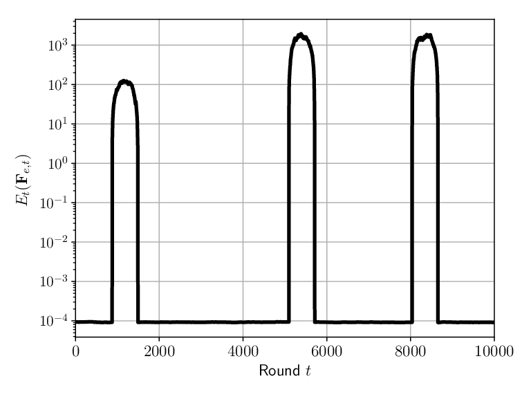
We now assume that the FCM changes with time. We replace with at time in Figure 4. We consider a observation noise and horizon . As previously mentioned, this could represent a scenario where electric vehicles can come and go at a parking garage. We set the time horizon to and consider different configurations during this time horizon as shown in Figure 6. Each of the four FCM configurations corresponds to a different duty cycle, as described in the previous section. The relative estimation error for the online case is given by
| (17) |
The results for the relative estimation error are presented in Figure 7. The estimator performs well except during brief transitions between configurations. This is because the measurement matrices have data from the previous configuration. To remedy this, the estimator could be combined with an event detection algorithm to omit prior measurements when a significant change is occurring.

VII-D Network reduction example
In this section, we apply the reduction theorem to the network Figure 2a and obtain the equivalent, virtual FCM of Figure 2b. Two FCMs, and are directly connected to node . Two other FCMs, at node and at node , are connected to node via lines with impedance and respectively.
We set the average value of the dc currents, resistances, susceptances according to Table I and according to [11, Table II]. To the each dc current, resistances, susceptances and components of , we add a zero-mean Gaussian noise with standard deviation given respectively by , , , . The four exact FCMs have the same internal parameters and randomly sampled switching sequences as in Section VII-B. We omit measurement noise as our objective is to validate the theoretical results of Section III.
We run tests. In each test, we compute the equivalent reduced FCM, , using Theorem 1 given all four FCMs and their dc input current. We estimate the equivalent reduced FCM, , using Section V with . The exact harmonic current is calculated using the network equations given the four FCMs, their dc currents and . The details for the computation of are given in Appendix A. We also compute the harmonic current obtained with the equivalent reduced FCM, , and that obtained from the estimated FCM, . Table III gives the mean FCM error as well as the following current error metrics:
All errors are effectively zero, in accordance with the theoretical results of Section III.
| Mean error | Value |
|---|---|
VIII Conclusion
We have presented basic approaches for estimating network parameters necessary for modeling harmonics. We have posed least squares problems for estimating the line admittances and FCMs, and an online algorithm for the latter case. We have also given a network reduction theorem, which enables one to model arbitrary, unobservable subtrees with a single, virtual FCM. We have validated all methods on a simple numerical example.
Appendix A Network equation solution
In this appendix, we solve for the relevant electrical quantities in the -FCM network in Figure 2a. All voltages are the same at a given node, and hence . By Kirchhoff’s current law, we have and . There are 8 unknown vectors: , , , , , , . We set as our input data.
For the 4-FCM network, we have the following equations. By Kirchhoff’s current law at node , we have
| (18) |
Using Ohm’s law on line , we obtain:
| (19) |
and for line ,
| (20) |
We apply the FCM relation at the three nodes:
| (21) | ||||
| (22) | ||||
| (23) | ||||
| (24) |
References
- [1] J. Arrillaga and N. R. Watson, Power system harmonics. John Wiley & Sons, 2004.
- [2] J. M. Carrasco, L. G. Franquelo, J. T. Bialasiewicz, E. Galván, R. C. Portillo Guisado, M. M. Prats, J. I. León, and N. Moreno-Alfonso, “Power-electronic systems for the grid integration of renewable energy sources: A survey,” IEEE Transactions on Industrial Electronics, vol. 53, no. 4, pp. 1002–1016, 2006.
- [3] G. M. Masters, Renewable and efficient electric power systems. John Wiley & Sons, 2013.
- [4] F. De La Rosa, Harmonics and power systems. CRC Press Boca Raton, 2006.
- [5] R. D. Henderson and P. J. Rose, “Harmonics: The effects on power quality and transformers,” IEEE Transactions on Industry Applications, vol. 30, no. 3, pp. 528–532, 1994.
- [6] P. Gray and P. Lehn, “Time-domain derived frequency-domain voltage source converter model for harmonic analysis,” in Harmonics and Quality of Power (ICHQP), 15th International Conference on. IEEE, 2012, pp. 512–517.
- [7] K. L. Lian and P. Lehn, “Steady-state simulation methods of closed-loop power converter systems—a systematic solution procedure,” IEEE Transactions on Circuits and Systems I: Regular Papers, vol. 59, no. 6, pp. 1299–1311, 2012.
- [8] N. Rajagopal and J. Quaicoe, “Harmonic analysis of three-phase ac/dc converters using the harmonic admittance method,” in Electrical and Computer Engineering, Canadian Conference on. IEEE, 1993, pp. 313–316.
- [9] M. Fauri, “Harmonic modelling of non-linear load by means of crossed frequency admittance matrix,” IEEE Transactions on Power Systems, vol. 12, no. 4, pp. 1632–1638, 1997.
- [10] Y. Sun, G. Zhang, W. Xu, and J. G. Mayordomo, “A harmonically coupled admittance matrix model for ac/dc converters,” IEEE Transactions on Power Systems, vol. 22, no. 4, pp. 1574–1582, 2007.
- [11] P. Lehn and K. Lian, “Frequency coupling matrix of a voltage-source converter derived from piecewise linear differential equations,” IEEE Transactions on Power Delivery, vol. 22, no. 3, pp. 1603–1612, 2007.
- [12] F. Yahyaie, P. Gray, and P. Lehn, “Application of experimentally measured frequency coupling matrices for improved harmonic estimation,” in Proc. 9th Annual CIGRÉ Canada Conf., 2014, pp. 290–294.
- [13] X. J. Zong, P. A. Gray, and P. W. Lehn, “New metric recommended for IEEE Standard 1547 to limit harmonics injected into distorted grids,” IEEE Transactions on Power Delivery, vol. 31, no. 3, pp. 963–972, 2016.
- [14] F. Yahyaie and P. W. Lehn, “Using frequency coupling matrix techniques for the analysis of harmonic interactions,” IEEE Transactions on Power Delivery, vol. 31, no. 1, pp. 112–121, 2016.
- [15] M. Saadeh, M. Alsarray, and R. McCann, “Estimation of the bus admittance matrix for transmission systems from synchrophasor data,” in Transmission and Distribution Conference and Exposition (T&D), 2016 IEEE/PES, pp. 1–5.
- [16] Y. Tian, J. A. Taylor, and N. Li, “Harmonic reduction via optimal power flow and the frequency coupling matrix,” in Control Technology and Applications (CCTA), 2017 IEEE Conference on, pp. 2150–2157.
- [17] E. Larsen, D. Baker, and J. McIver, “Low-order harmonic interactions on ac/dc systems,” IEEE Transactions on Power Delivery, vol. 4, no. 1, pp. 493–501, 1989.
- [18] S. Jalali and R. Lasseter, “Harmonic interaction of power systems with static switching circuits,” in Power Electronics Specialists Conference, 22nd Annual IEEE, 1991, pp. 330–337.
- [19] C. Saniter, A. Wood, R. Hanitsch, and D. Schulz, “Modelling the effects of AC system impedance unbalance on PWM converters using frequency coupling matrices,” in Power Tech Conference Proceedings, IEEE Bologna, vol. 2, 2003, pp. 1–6.
- [20] L. Hu and R. Yacamini, “Harmonic transfer through converters and hvdc links,” IEEE Transactions on Power Electronics, vol. 7, no. 3, pp. 514–525, 1992.
- [21] M. Bazrafshan and N. Gatsis, “Comprehensive modeling of three-phase distribution systems via the bus admittance matrix,” IEEE Transactions on Power Systems, vol. 33, no. 2, pp. 2015–2029, 2018.
- [22] O. Ardakanian, V. W. Wong, R. Dobbe, S. H. Low, A. von Meier, C. Tomlin, and Y. Yuan, “On identification of distribution grids,” arXiv preprint arXiv:1711.01526, 2017.
- [23] A. Carta, N. Locci, and C. Muscas, “A PMU for the measurement of synchronized harmonic phasors in three-phase distribution networks,” IEEE Transactions on Instrumentation and Measurement, vol. 58, no. 10, pp. 3723–3730, 2009.
- [24] S. K. Jain, P. Jain, and S. N. Singh, “A fast harmonic phasor measurement method for smart grid applications,” IEEE Transactions on Smart Grid, vol. 8, no. 1, pp. 493–502, 2017.
- [25] I. D. Melo, J. L. Pereira, A. M. Variz, and P. A. Garcia, “Harmonic state estimation for distribution networks using phasor measurement units,” Electric Power Systems Research, vol. 147, pp. 133–144, 2017.
- [26] A. G. Phadke and J. S. Thorp, Synchronized phasor measurements and their applications. Springer, 2008.
- [27] K. Martin, D. Hamai, M. Adamiak, S. Anderson, M. Begovic, G. Benmouyal, G. Brunello, J. Burger, J. Cai, B. Dickerson et al., “Exploring the IEEE standard C37. 118–2005 synchrophasors for power systems,” IEEE Transactions on Power Delivery, vol. 23, no. 4, pp. 1805–1811, 2008.
- [28] A. Abur and A. G. Exposito, Power system state estimation: theory and implementation. CRC Press, 2004.
- [29] G. Krumpholz, K. Clements, and P. Davis, “Power system observability: a practical algorithm using network topology,” IEEE Transactions on Power Apparatus and Systems, no. 4, pp. 1534–1542, 1980.
- [30] J. Sherman and W. J. Morrison, “Adjustment of an inverse matrix corresponding to a change in one element of a given matrix,” The Annals of Mathematical Statistics, vol. 21, no. 1, pp. 124–127, 1950.
- [31] W. W. Hager, “Updating the inverse of a matrix,” SIAM Review, vol. 31, no. 2, pp. 221–239, 1989.