跳到论文正文
W Papers独立论文阅读器 arXiv:1809.08099 论文正文 计算阅读时间 · 0%
引用这篇论文根据当前论文元数据生成,正式投稿前建议核对。


License: arXiv.org perpetual non-exclusive license
arXiv:1809.08099v1 [math.AP] 21 Sep 2018

WKB expansion for a fractional Schrödinger equation with applications to controllability

Umberto Biccari ††thanks: DeustoTech, University of Deusto, 48007 Bilbao, Basque Country, Spain.††thanks: Facultad Ingeniería, Universidad de Deusto, Avda Universidades 24, 48007 Bilbao, Basque Country, Spain. Email: umberto.biccari@deusto.es    Alejandro B. Aceves ††thanks: Southern Methodist University, Dedman College of Humanities and Sciences, PO Box 750235, Dallas, Texas, United States. Email: aaceves@smu.edu
Abstract

This paper is devoted to the analysis of propagation properties for the solutions of a one-dimensional non-local Schrödinger equation involving the fractional Laplace operator (−dx 2)s(-d_{x}^{\,2})^{s}, s∈(0,1)s\in(0,1). We adopt a classical WKB approach and we provide a systematic procedure for building a suitable ansatz for the solutions to the problem. In this way, we can obtain quasi-solutions which are localized along the rays of geometric optics, whose group velocity can be computed explicitly in terms of the parameter ss. Our results are then confirmed by numerical simulations, based on a finite element approximation of the fractional Laplacian and on a Crank-Nicholson scheme for the time integration. As an application, the controllability problem for the fractional Schrödinger equation is analyzed, finding confirmations of previously known results.
Keywords: WKB, fractional Laplacian, Schrödinger equation, propagation of solutions.
Mathematics Subject Classification (2010): 35A35, 35Q41, 35Q60, 78A05.

1 Introduction

In this paper, we are interested in the construction of ray-like solutions in geometric optics for the following one-dimensional non-local equation

𝒫su:=[i∂t+(−dx 2)s]u=0,(x,t)∈ℝ×(0,+∞),\mathcal{P}_{s}u:=\left[i\partial_{t}+(-d_{x}^{\,2})^{s}\right]u=0,\;\;\;\;(x,t)\in\mathbb{R}\times(0,+\infty), (1.1)

with highly oscillatory initial datum

u⁡(x,0)=uin​(x)​ei​ξ0ε​x:=u0​(x),ξ0∈ℝ.u(x,0)=u_{\textrm{\small in}}(x)e^{i\frac{\xi_{0}}{\varepsilon}x}:=u_{0}(x),\;\;\;\xi_{0}\in\mathbb{R}. (1.2)

In (1.1), (−dx 2)s(-d_{x}^{\,2})^{s} is the fractional Laplacian, defined for all s∈(0,1)s\in(0,1) and for any function ff sufficiently smooth as the following singular integral

(−dx 2)s​f​(x):=c1,s​P.V.∫ℝf⁡(x)−f⁡(y)|x−y|1+2​s​𝑑y,\displaystyle(-d_{x}^{\,2})^{s}f(x):=c_{1,s}\;P.V.\int_{\mathbb{R}}\frac{f(x)-f(y)}{|x-y|^{1+2s}}\,dy,

with c1,sc_{1,s} a normalization constant given by (see [11, Section 3] and [27, Appendix A])

c1,s:=(∫ℝ1−cos⁡(z)|z|1+2​s​𝑑z)−1=s​22​s​Γ​(s+12)π​Γ​(1−s),c_{1,s}:=\left(\int_{\mathbb{R}}\frac{1-\cos(z)}{|z|^{1+2s}}\,dz\right)^{-1}=\frac{s2^{2s}\Gamma\left(s+\frac{1}{2}\right)}{\sqrt{\pi}\Gamma(1-s)}, (1.3)

where Γ\Gamma is the usual Gamma function. The parameter ε\varepsilon in (1.2) represents the typical wavelength of oscillations of the initial data, which in turn will affect the solution form of (1.1). Moreover, we will assume the initial phase uinu_{\textrm{\small in}} to be an L2​(ℝ)L^{2}(\mathbb{R}) function, so that we have u0∈L2​(ℝ)u_{0}\in L^{2}(\mathbb{R}).

Space-fractional Schrödinger equations have been introduced by Laskin in quantum mechanics ([16, 17, 18]), since they provide a natural extension of the standard local model when the Brownian trajectories in Feynman path integrals are replaced by Levy flights, which are generated by the fractional Laplacian. Applications of (1.1) may be found in the study of a condensed-matter realization of Lévy crystals ([29]). More recently, the fractional Schrödinger equation was introduced into optics by Longhi in [23], with applications to laser implementation.

The present paper deals with the construction of asymptotic approximations in geometric optics for the solutions to (1.1), and with their application to the study of controllability problems.

Asymptotic analysis for wave-like equations through geometric optics (also known as the Wentzel-Kramers-Brillouin (WKB) method or ray-tracing, [7, 15, 28, 33]) is nowadays a classical tool that has been developed in several directions. An incomplete biography on the topic includes [20, 21, 22]. It is by now well-known that wave-type equations, in a local framework, have solutions that are localized near curves (t,x⁡(t))(t,x(t)) in space-time, also called rays. These curves are, in the interior of the domain of definition of the equation, solutions of a Hamiltonian system of ordinary differential equations which involves the coefficients of the operator. When one of these trajectories hits the boundary of the domain it is reflected according to the classical laws of optics.

With this observation in mind, asymptotic methods allow to study the behavior of several wave-type phenomena, with applications, e.g., in geophysics ([10, 12]), acoustic wave equations ([19, 30]) or gravity waves ([31]).

To the best of our knowledge, a WKB approach has not yet been fully developed in a non-local setting. On the other hand, this is certainly an interesting issue, not only from a purely mathematical perspective, but also due to the several applications that we mentioned above. Our work represents a first step in this direction, providing a complete procedure for obtaining a WKB expansion of equation (1.1). In more detail, we will show that given a ray (t,x⁡(t))(t,x(t)) it is possible to construct quasi-solutions of the fractional Schrödinger equation (1.1) such that the amount of their energy outside a ball of radius ε14\varepsilon^{\frac{1}{4}} centered at x⁡(t)x(t) is of the order of ε14\varepsilon^{\frac{1}{4}}.

A motivation and a natural application for our construction will then be the study of controllability properties for the one dimensional fractional Schrödinger equation

{i​ut+(−dx 2)s​u=g​χω×(0,T),(x,t)∈(−1,1)×(0,T)u≡0,(x,t)∈(−1,1)c×(0,T)u⁡(x,0)=u0​(x),x∈(−1,1),\displaystyle\begin{cases}iu_{t}+(-d_{x}^{\,2})^{s}u=g\chi_{\omega\times(0,T)},&(x,t)\in(-1,1)\times(0,T)\\ u\equiv 0,&(x,t)\in(-1,1)^{c}\times(0,T)\\ u(x,0)=u_{0}(x),&x\in(-1,1),\end{cases} (1.4)

where ω\omega is a subset of the space domain (−1,1)(-1,1). As we already proved in [3] by means of spectral analysis techniques, for (1.4) we have the following control properties:

  • ∙\bullet

    For s>1/2s>1/2, null controllability holds in any finite time T>0T>0. In other words, given any u0∈L2​(−1,1)u_{0}\in L^{2}(-1,1) there exists a control function g∈L2​(ω×(0,T))g\in L^{2}(\omega\times(0,T)) such that the solution to (1.4) satisfies u⁡(x,T)=0u(x,T)=0.

  • ∙\bullet

    For s=1/2s=1/2, the same result holds if we assume the controllability time TT to be large enough, i.e T≥T0>0T\geq T_{0}>0.

  • ∙\bullet

    For s<1/2s<1/2, the equation (1.4) is not null controllable.

Through the construction of localized solution that we are going to present in this work, it will be possible to give a further confirmation to the above facts.

The approach that we are going to use for building localized solutions is quite standard. In particular, given a plane wave solution uεu^{\,\varepsilon}, we will look for quasi-solutions to (1.1) with an ansatz of the type

zε​(x,t)=uε​(x,t)​aε​(x,t),aε​(x,t)=∑j≥0εp​j​aj​(x,t),\displaystyle z^{\,\varepsilon}(x,t)=u^{\,\varepsilon}(x,t)a^{\,\varepsilon}(x,t),\;\;\;a^{\,\varepsilon}(x,t)=\sum_{j\geq 0}\varepsilon^{pj}a_{j}(x,t),

with p∈ℝp\in\mathbb{R}, and where the functions aja_{j} have to be determined. The identification of the aja_{j}-s will then be carried out imposing

𝒫s​zε=O⁡(ε∞),\displaystyle\mathcal{P}_{s}z^{\,\varepsilon}=O(\varepsilon^{\infty}),

thus obtaining a series of PDEs in which it will be possible to clearly separate the leading order terms, with respect to ε\varepsilon, from several remainders which will vanish as ε→0\varepsilon\to 0. This will generate a cascade system for the functions aja_{j}, which can then be determined as the solution of certain given Partial Differential Equations.

This paper is organized as follows. In Section 2, we will introduce some preliminary notion that we shall use in our analysis. In Section 3, we will present the construction of the ansatz for the asymptotic expansion of the solutions to our fractional Schrödinger equation 1.1. In Section 4, we will show that the quasi-solution zεz^{\,\varepsilon} obtained through our procedure is a good approximation of the real solutions uu to our original equation. Section 5 will be devoted to the discussion on the application of our methodology to the study of control properties. Finally, in Section 6, we will present some numerical simulations which confirm our theoretical results.

2 Preliminaries

Before presenting the construction of our ansatz, we introduce some preliminary facts that we are going to need for our further analysis.

First of all, a classical result on the Schrödinger equation tells us that for all s∈(0,1)s\in(0,1) the Hs​(ℝ)H^{s}(\mathbb{R})-norm of the solution uu to (1.1) is conserved. This is an easy consequence of the skew-adjointness of the operator i​(−dx 2)si(-d_{x}^{\,2})^{s}, which allows to readily check that

0=⟨ut−i​(−dx 2)s​u,u+(−dx 2)s​u⟩L2​(ℝ)=12​dd​t​(‖u‖L2​(ℝ)2+[u]Hs​(ℝ)2)=12​dd​t​‖u‖Hs​(ℝ)2.\displaystyle 0=\big\langle u_{t}-i(-d_{x}^{\,2})^{s}u,u+(-d_{x}^{\,2})^{s}u\big\rangle_{L^{2}(\mathbb{R})}=\frac{1}{2}\frac{d}{dt}\left({\left\|u\right\|}_{L^{2}(\mathbb{R})}^{2}+[u]_{H^{s}(\mathbb{R})}^{2}\right)=\frac{1}{2}\frac{d}{dt}{\left\|u\right\|}_{H^{s}(\mathbb{R})}^{2}.

In particular, ‖u‖Hs​(ℝ){\left\|u\right\|}_{H^{s}(\mathbb{R})} represents an energy for our equation.

Second, we recall here the definition of null bicharacteristics, which will have a fundamental role in our later construction.

Given a general pseudo-differential operator Ψ\Psi with principal symbol ψ=ψ⁡(x,t,ξ,τ)\psi=\psi(x,t,\xi,\tau), a null bicharacteristic is defined to be a solution of the following system of ordinary differential equations

{x˙​(σ)=ψξ​(x⁡(σ),t⁡(σ),ξ⁡(σ),τ⁡(σ))t˙​(σ)=ψτ​(x⁡(σ),t⁡(σ),ξ⁡(σ),τ⁡(σ))ξ˙​(σ)=−ψx​(x⁡(σ),t⁡(σ),ξ⁡(σ),τ⁡(σ))τ˙​(σ)=−ψt​(x⁡(σ),t⁡(σ),ξ⁡(σ),τ⁡(σ))\displaystyle\begin{cases}\dot{x}(\sigma)=\psi_{\xi}(x(\sigma),t(\sigma),\xi(\sigma),\tau(\sigma))\\ \dot{t}(\sigma)=\psi_{\tau}(x(\sigma),t(\sigma),\xi(\sigma),\tau(\sigma))\\ \dot{\xi}(\sigma)=-\psi_{x}(x(\sigma),t(\sigma),\xi(\sigma),\tau(\sigma))\\ \dot{\tau}(\sigma)=-\psi_{t}(x(\sigma),t(\sigma),\xi(\sigma),\tau(\sigma))\end{cases}

with initial data (x⁡(0),t⁡(0),ξ⁡(0),τ⁡(0))=(x0,t0,ξ0,τ0)∈ℝ4(x(0),t(0),\xi(0),\tau(0))=(x_{0},t_{0},\xi_{0},\tau_{0})\in\mathbb{R}^{4} where the value of τ0∈ℝ\tau_{0}\in\mathbb{R} is chosen so that ψ⁡(x0,t0,ξ0,τ0)=0\psi(x_{0},t_{0},\xi_{0},\tau_{0})=0. Then, the projection of a null bicharacteristic to the physical time-space, (t,x⁡(t))(t,x(t)), traces a curve in (0,+∞)×ℝ(0,+\infty)\times\mathbb{R} which is called a ray of Ψ\Psi.

In the case of our fractional Schrödinger equation, notice that 𝒫s=i∂t+(−dx 2)s\mathcal{P}_{s}=i\partial_{t}+(-d_{x}^{\,2})^{s} is a pseudo-differential operator with symbol ps​(x,t,ξ,τ)=τ−|ξ|2​sp_{s}(x,t,\xi,\tau)=\tau-|\xi|^{2s}. Therefore, the bicharacteristic system is given by

{x˙​(σ)=±2​s​|ξ⁡(σ)|2​s−1,x⁡(0)=x0t˙​(σ)=1,t⁡(0)=t0ξ˙​(σ)=0,ξ⁡(0)=ξ0τ˙​(σ)=0,τ⁡(0)=|ξ0|2​s.\displaystyle\begin{cases}\dot{x}(\sigma)=\pm 2s|\xi(\sigma)|^{2s-1},&x(0)=x_{0}\\ \dot{t}(\sigma)=1,&t(0)=t_{0}\\ \dot{\xi}(\sigma)=0,&\xi(0)=\xi_{0}\\ \dot{\tau}(\sigma)=0,&\tau(0)=|\xi_{0}|^{2s}.\end{cases} (2.1)

Moreover, without losing generality we may assume t0=0t_{0}=0. Then, (2.1) can be solved explicitly, and we obtain the following expressions for the bicharacteristics

{x⁡(σ)=x0±2​s​|ξ0|2​s−1​σt⁡(σ)=σξ⁡(σ)=ξ0τ⁡(σ)=|ξ0|2​s.\displaystyle\begin{cases}x(\sigma)=x_{0}\pm 2s|\xi_{0}|^{2s-1}\sigma\\ t(\sigma)=\sigma\\ \xi(\sigma)=\xi_{0}\\ \tau(\sigma)=|\xi_{0}|^{2s}.\end{cases}

In particular, the rays of 𝒫s\mathcal{P}_{s} are given by the curves (t,x0±2​s​|ξ0|2​s−1​t)∈(0,+∞)×ℝ(t,x_{0}\pm 2s|\xi_{0}|^{2s-1}t)\in(0,+\infty)\times\mathbb{R}. Notice that, as one expects since the operator has constant coefficients, these rays are straight lines.

3 Construction of the ansatz

This section is devoted to a heuristic exposition of the key ideas leading to the construction of ray-like solutions for our equation. We begin by seeking approximate solutions with an ansatz of WKB type with linear phase:

zε​(x,t)=c⁡(ε)​uε​(x,t)​aε​(x,t),aε​(x,t)=∑j≥0εp​j​aj​(x,t),\displaystyle z^{\,\varepsilon}(x,t)=c(\varepsilon)u^{\,\varepsilon}(x,t)a^{\,\varepsilon}(x,t),\;\;\;a^{\,\varepsilon}(x,t)=\sum_{j\geq 0}\varepsilon^{pj}a_{j}(x,t), (3.1)

where p∈ℝp\in\mathbb{R} and the functions aja_{j} have to be determined. The constant c⁡(ε)c(\varepsilon), instead, will be chosen asking that the function zεz^{\,\varepsilon} has Hs​(ℝ)H^{s}(\mathbb{R})-norm of the order 𝒪⁡(1)\mathcal{O}(1). We start by observing that, since for any ξ0∈ℝ\xi_{0}\in\mathbb{R} we have

(−dx 2)s​ei​ξ0​ε−1​x=|ξ0|2​s​ε−2​s​ei​ξ0​ε−1​x,\displaystyle(-d_{x}^{\,2})^{s}e^{i\xi_{0}\varepsilon^{-1}x}=|\xi_{0}|^{2s}\varepsilon^{-2s}e^{i\xi_{0}\varepsilon^{-1}x}, (3.2)

the plane wave

uε​(x,t):=ei⁡[ξ0​ε−1​x+|ξ0|2​s​ε−2​s​t]\displaystyle u^{\,\varepsilon}(x,t):=e^{i\left[\xi_{0}\varepsilon^{-1}x\,+\,|\xi_{0}|^{2s}\varepsilon^{-2s}t\,\right]}

satisfies 𝒫s​uε=0\mathcal{P}_{s}u^{\,\varepsilon}=0. Notice that

ei⁡[ξ0​ε−1​x+|ξ0|2​s​ε−2​s​t]=ei​ξ0​ε−1​(x−ε1−2​s2​s​x​(t)).\displaystyle e^{i\left[\xi_{0}\varepsilon^{-1}x\,+\,|\xi_{0}|^{2s}\varepsilon^{-2s}t\,\right]}=e^{i\xi_{0}\varepsilon^{-1}\left(x\,-\,\frac{\varepsilon^{1-2s}}{2s}x(t)\,\right)}.

At this point, for identifying the correct value of the parameter pp in (3.1), and for determining the functions aja_{j}, we need to compute 𝒫s​zε\mathcal{P}_{s}z^{\,\varepsilon} and gather the terms that we obtain according to their order with respect to ε\varepsilon. Moreover, in what follows we shall employ the following expression for the fractional Laplacian of the product of two functions

(−dx 2)s​(f​g)=f​(−dx 2)s​g+g​(−dx 2)s​f−Is​(f,g),\displaystyle(-d_{x}^{\,2})^{s}(fg)=f(-d_{x}^{\,2})^{s}g+g(-d_{x}^{\,2})^{s}f-I_{s}(f,g), (3.3)

where the term IsI_{s} is given by (see, e.g., [6, 27])

Is​(f,g)​(x):=c1,s​P.V.∫ℝN(f⁡(x)−f⁡(y))​(g⁡(x)−g⁡(y))|x−y|1+2​s​𝑑y.\displaystyle I_{s}(f,g)(x):=c_{1,s}\,P.V.\int_{\mathbb{R}^{N}}\frac{(f(x)-f(y))(g(x)-g(y))}{|x-y|^{1+2s}}\,dy.

By means of (3.2) and (3.3), we can immediately see that

𝒫s​zε=c⁡(ε)​uε​[i​aε+(−dx 2)s​aε−Ks​(aε)]\displaystyle\mathcal{P}_{s}z^{\,\varepsilon}=c(\varepsilon)u^{\,\varepsilon}\Big[ia^{\,\varepsilon}+(-d_{x}^{\,2})^{s}a^{\,\varepsilon}-K_{s}(a^{\,\varepsilon})\Big] (3.4)

with

Ks​(aε)\displaystyle K_{s}(a^{\,\varepsilon}) =c1,s​P.V.∫ℝ1−ei​ξ0ε​(y−x)|x−y|1+2​s​[aε​(x,t)−aε​(y,t)]​𝑑y\displaystyle=\displaystyle c_{1,s}\,P.V.\int_{\mathbb{R}}\frac{1-e^{i\frac{\xi_{0}}{\varepsilon}(y-x)}}{|x-y|^{1+2s}}\Big[a^{\,\varepsilon}(x,t)-a^{\,\varepsilon}(y,t)\Big]\,dy
=c1,s​ξ02​sε2​s​P.V.∫ℝ1−ei​q|q|1+2​s​[aε​(x,t)−aε​(x+εξ0​q,t)]​𝑑q.\displaystyle=\displaystyle c_{1,s}\frac{\xi_{0}^{2s}}{\varepsilon^{2s}}\,P.V.\int_{\mathbb{R}}\frac{1-e^{iq}}{|q|^{1+2s}}\bigg[a^{\,\varepsilon}(x,t)-a^{\,\varepsilon}\left(x+\frac{\varepsilon}{\xi_{0}}q,t\right)\bigg]\,dq.

Now, employing a fractional Taylor expansion ([14, 32]), for any β∈(0,1)\beta\in(0,1) and x≤θ≤x+εξ0​qx\leq\theta\leq x+\frac{\varepsilon}{\xi_{0}}q we can write

aε​(x+εξ0​q,t)=aε​(x,t)+𝒟β​aε​(x,t)Γ⁡(1+β)​(εξ0​q)β+𝒟2​β​aε​(x,t)Γ⁡(1+2​β)​(εξ0​q)2​β+𝒟3​β​aε​(θ,t)Γ⁡(1+3​β)​(εξ0​q)3​β,\displaystyle\displaystyle a^{\,\varepsilon}\left(x+\frac{\varepsilon}{\xi_{0}}q,t\right)=a^{\,\varepsilon}(x,t)+\frac{\mathcal{D}^{\,\beta}a^{\,\varepsilon}(x,t)}{\Gamma(1+\beta)}\left(\frac{\varepsilon}{\xi_{0}}q\right)^{\beta}+\frac{\mathcal{D}^{2\beta}a^{\,\varepsilon}(x,t)}{\Gamma(1+2\beta)}\left(\frac{\varepsilon}{\xi_{0}}q\right)^{2\beta}+\frac{\mathcal{D}^{3\beta}a^{\,\varepsilon}(\theta,t)}{\Gamma(1+3\beta)}\left(\frac{\varepsilon}{\xi_{0}}q\right)^{3\beta}, (3.5)

where with 𝒟β\mathcal{D}^{\,\beta} we indicate the following fractional derivative of order β\beta

𝒟β​f​(x):=1Γ⁡(1−β)​∫−∞xf′​(y)(x−y)β​𝑑y,β∈(0,1).\displaystyle\mathcal{D}^{\,\beta}f(x):=\frac{1}{\Gamma(1-\beta)}\int_{-\infty}^{x}\frac{f^{\prime}(y)}{(x-y)^{\beta}}\,dy,\;\;\;\beta\in(0,1).

Thanks to (3.5), we get

Ks​(aε)=\displaystyle K_{s}(a^{\,\varepsilon})= −c1,s​ξ02​s−βΓ⁡(1+β)​εβ−2​s​𝒟β​aε​(x,t)​P.V.∫ℝ1−ei​q|q|1+2​s​qβ​𝑑q\displaystyle\displaystyle-c_{1,s}\frac{\xi_{0}^{2s-\beta}}{\Gamma(1+\beta)}\varepsilon^{\beta-2s}\mathcal{D}^{\,\beta}a^{\,\varepsilon}(x,t)\,P.V.\int_{\mathbb{R}}\frac{1-e^{iq}}{|q|^{1+2s}}q^{\beta}\,dq
−c1,s​ξ02​s−2​βΓ⁡(1+2​β)​ε2​β−2​s​𝒟2​β​aε​(x,t)​P.V.∫ℝ1−ei​q|q|1+2​s​q2​β​𝑑q\displaystyle\displaystyle-c_{1,s}\frac{\xi_{0}^{2s-2\beta}}{\Gamma(1+2\beta)}\varepsilon^{2\beta-2s}\mathcal{D}^{2\beta}a^{\,\varepsilon}(x,t)\,P.V.\int_{\mathbb{R}}\frac{1-e^{iq}}{|q|^{1+2s}}q^{2\beta}\,dq
−c1,s​ξ02​s−3​βΓ⁡(1+3​β)​ε2​β−3​s​𝒟3​β​aε​(θ,t)​P.V.∫ℝ1−ei​q|q|1+2​s​q3​β​𝑑q.\displaystyle\displaystyle-c_{1,s}\frac{\xi_{0}^{2s-3\beta}}{\Gamma(1+3\beta)}\varepsilon^{2\beta-3s}\mathcal{D}^{3\beta}a^{\,\varepsilon}(\theta,t)\,P.V.\int_{\mathbb{R}}\frac{1-e^{iq}}{|q|^{1+2s}}q^{3\beta}\,dq.

Moreover, we observe that since |1−ei​q|=2−2​cos⁡(q)|1-e^{iq}|=2-2\cos(q), for all q∈ℝq\in\mathbb{R} and β<2​s/3\beta<2s/3 the integrals in the above expression are finite. In particular, we have

∙|P.V.∫ℝ1−ei​q|q|1+2​sqβdq|≤4Γ(β−2s−1)cos[(2​s−β)​π2],\displaystyle\displaystyle\bullet\;\;\left|P.V.\int_{\mathbb{R}}\frac{1-e^{iq}}{|q|^{1+2s}}q^{\beta}\,dq\,\right|\leq 4\Gamma(\beta-2s-1)\cos\left[\frac{(2s-\beta)\pi}{2}\right],
∙|P.V.∫ℝ1−ei​q|q|1+2​sq2​βdq|≤4Γ(2β−2s−1)cos[(s−β)π],\displaystyle\displaystyle\bullet\;\;\left|P.V.\int_{\mathbb{R}}\frac{1-e^{iq}}{|q|^{1+2s}}q^{2\beta}\,dq\,\right|\leq 4\Gamma(2\beta-2s-1)\cos\big[(s-\beta)\pi\big],
∙|P.V.∫ℝ1−ei​q|q|1+2​sq3​βdq|≤4Γ(3β−2s−1)cos[(2​s−3​β)​π2].\displaystyle\displaystyle\bullet\;\;\left|P.V.\int_{\mathbb{R}}\frac{1-e^{iq}}{|q|^{1+2s}}q^{3\beta}\,dq\,\right|\leq 4\Gamma(3\beta-2s-1)\cos\left[\frac{(2s-3\beta)\pi}{2}\right].

Therefore, we can rewrite

Ks​(aε)=−𝒞β​εβ−2​s​𝒟β​aε​(x,t)−𝒞2​β​ε2​β−2​s​𝒟2​β​aε​(x,t)−𝒞3​β​ε3​β−2​s​𝒟3​β​aε​(θ,t),\displaystyle K_{s}(a^{\,\varepsilon})=-\mathcal{C}_{\beta}\varepsilon^{\beta-2s}\mathcal{D}^{\,\beta}a^{\,\varepsilon}(x,t)-\mathcal{C}_{2\beta}\varepsilon^{2\beta-2s}\mathcal{D}^{2\beta}a^{\,\varepsilon}(x,t)-\mathcal{C}_{3\beta}\varepsilon^{3\beta-2s}\mathcal{D}^{3\beta}a^{\,\varepsilon}(\theta,t),

with

𝒞γ:=c1,s​ξ02​s−γΓ⁡(1+γ)​P.V.∫ℝ1−ei​q|q|1+2​s​qγ​𝑑q,\displaystyle\mathcal{C}_{\gamma}:=c_{1,s}\frac{\xi_{0}^{2s-\gamma}}{\Gamma(1+\gamma)}P.V.\int_{\mathbb{R}}\frac{1-e^{iq}}{|q|^{1+2s}}q^{\gamma}\,dq,

and we then obtain

𝒫szε(x,t)=c(ε)uε[iatε(x,t)+(−dx 2)saε(x,t)\displaystyle\mathcal{P}_{s}z^{\,\varepsilon}(x,t)=c(\varepsilon)u^{\,\varepsilon}\Big[ia^{\,\varepsilon}_{t}(x,t)+(-d_{x}^{\,2})^{s}a^{\,\varepsilon}(x,t) +𝒞β​εβ−2​s​𝒟β​aε​(x,t)\displaystyle+\mathcal{C}_{\beta}\varepsilon^{\beta-2s}\mathcal{D}^{\,\beta}a^{\,\varepsilon}(x,t)
+𝒞2​βε2​β−2​s𝒟2​βaε(x,t)+𝒞3​βε3​β−2​s𝒟3​βaε(θ,t)].\displaystyle+\mathcal{C}_{2\beta}\varepsilon^{2\beta-2s}\mathcal{D}^{2\beta}a^{\,\varepsilon}(x,t)+\mathcal{C}_{3\beta}\varepsilon^{3\beta-2s}\mathcal{D}^{3\beta}a^{\,\varepsilon}(\theta,t)\Big].

Furthermore, let us introduce the following rescaling of the time variable t↦τ:=ε2​s−β​tt\mapsto\tau:=\varepsilon^{2s-\beta}t. In this way, (3.4) finally becomes

𝒫s​zε=c⁡(ε)​εβ−2​s​uε​∑j≥0εp​j​[i​∂τaj+𝒞β​𝒟β​aj+ε2​s−β​(−dx 2)s​aj+𝒞2​β​εβ​𝒟2​β​aj+𝒞3​β​ε2​β​𝒟3​β​aj​(θ,τ)].\displaystyle\mathcal{P}_{s}z^{\,\varepsilon}=c(\varepsilon)\varepsilon^{\beta-2s}u^{\,\varepsilon}\sum_{j\geq 0}\varepsilon^{pj}\Big[i\partial_{\tau}a_{j}+\mathcal{C}_{\beta}\mathcal{D}^{\,\beta}a_{j}+\varepsilon^{2s-\beta}(-d_{x}^{\,2})^{s}a_{j}+\mathcal{C}_{2\beta}\varepsilon^{\beta}\mathcal{D}^{2\beta}a_{j}+\mathcal{C}_{3\beta}\varepsilon^{2\beta}\mathcal{D}^{3\beta}a_{j}(\theta,\tau)\Big]. (3.6)

For determining from (3.6) the expression of the functions aja_{j}, we will now impose, for any j≥0j\geq 0,

𝒫s​zε=O⁡(ε∞),\displaystyle\mathcal{P}_{s}z^{\,\varepsilon}=O(\varepsilon^{\infty}),

thus obtaining a series of PDEs in which will be possible to clearly separate the leading order terms, with respect to ε\varepsilon, from several remainders which will vanish as ε→0\varepsilon\to 0. During this procedure, we will also identify the values of the parameters pp and β\beta that we shall employ.

Let us start firstly with j=0j=0. In this case, it is trivial to identify the leading equation, and we immediately have that the function a0​(x,τ)a_{0}(x,\tau) has to satisfy

i​∂τa0+𝒞β​𝒟β​a0=0.\displaystyle i\partial_{\tau}a_{0}+\mathcal{C}_{\beta}\mathcal{D}^{\beta}a_{0}=0. (3.7)

For j=1j=1, instead, choosing p=βp=\beta we obtain from (3.6) and (3.7)

εβ[i∂τa1+𝒞β𝒟βa1+𝒞2​β𝒟2​βa0\displaystyle\varepsilon^{\beta}\Big[i\partial_{\tau}a_{1}+\mathcal{C}_{\beta}\mathcal{D}^{\,\beta}a_{1}+\mathcal{C}_{2\beta}\mathcal{D}^{2\beta}a_{0} +ε2​s−2​β​(−dx 2)s​a0+𝒞3​β​εβ​𝒟3​β​a0​(θ,τ)\displaystyle+\varepsilon^{2s-2\beta}(-d_{x}^{\,2})^{s}a_{0}+\mathcal{C}_{3\beta}\varepsilon^{\beta}\mathcal{D}^{3\beta}a_{0}(\theta,\tau)
+ε2​s−β(−dx 2)sa1+𝒞2​βεβ𝒟2​βa1+𝒞3​βε2​β𝒟3​βa1(θ,τ)],\displaystyle+\varepsilon^{2s-\beta}(-d_{x}^{\,2})^{s}a_{1}+\mathcal{C}_{2\beta}\varepsilon^{\beta}\mathcal{D}^{2\beta}a_{1}+\mathcal{C}_{3\beta}\varepsilon^{2\beta}\mathcal{D}^{3\beta}a_{1}(\theta,\tau)\Big],

and we thus find that the function a1​(x,τ)a_{1}(x,\tau) has to satisfy

i​∂τa1+𝒞β​𝒟β​a1+𝒞2​β​𝒟2​β​a0=0.\displaystyle i\partial_{\tau}a_{1}+\mathcal{C}_{\beta}\mathcal{D}^{\,\beta}a_{1}+\mathcal{C}_{2\beta}\mathcal{D}^{2\beta}a_{0}=0. (3.8)

Let us now continue with j=2j=2. In this case, we have

ε2​β[ε−2​β\displaystyle\varepsilon^{2\beta}\Big[\varepsilon^{-2\beta} (i​∂τa0+𝒞β​𝒟β​a0)⏟=0+ε2​s−3​β​(−dx 2)s​a0+𝒞3​β​𝒟3​β​a0​(θ,τ)\displaystyle\underbrace{(i\partial_{\tau}a_{0}+\mathcal{C}_{\beta}\mathcal{D}^{\,\beta}a_{0})}_{=0}+\varepsilon^{2s-3\beta}(-d_{x}^{\,2})^{s}a_{0}+\mathcal{C}_{3\beta}\mathcal{D}^{3\beta}a_{0}(\theta,\tau)
+ε−β​(i​∂τa1+𝒞β​𝒟β​a1+𝒞2​β​𝒟2​β​a0)⏟=0+ε2​s−2​β​(−dx 2)s​a1+𝒞3​β​εβ​𝒟3​β​a1​(θ,τ)+𝒞2​β​𝒟2​β​a1\displaystyle+\varepsilon^{-\beta}\underbrace{(i\partial_{\tau}a_{1}+\mathcal{C}_{\beta}\mathcal{D}^{\,\beta}a_{1}+\mathcal{C}_{2\beta}\mathcal{D}^{2\beta}a_{0})}_{=0}+\varepsilon^{2s-2\beta}(-d_{x}^{\,2})^{s}a_{1}+\mathcal{C}_{3\beta}\varepsilon^{\beta}\mathcal{D}^{3\beta}a_{1}(\theta,\tau)+\mathcal{C}_{2\beta}\mathcal{D}^{2\beta}a_{1}
+i∂τa2+𝒞β𝒟βa2+ε2​s−β(−dx 2)sa2+𝒞2​βεβ𝒟2​βa2+𝒞3​βε2​β𝒟3​βa2(θ,τ)].\displaystyle+i\partial_{\tau}a_{2}+\mathcal{C}_{\beta}\mathcal{D}^{\,\beta}a_{2}+\varepsilon^{2s-\beta}(-d_{x}^{\,2})^{s}a_{2}+\mathcal{C}_{2\beta}\varepsilon^{\beta}\mathcal{D}^{2\beta}a_{2}+\mathcal{C}_{3\beta}\varepsilon^{2\beta}\mathcal{D}^{3\beta}a_{2}(\theta,\tau)\Big].

and we thus find that the function a2​(x,τ)a_{2}(x,\tau) has to satisfy

i​∂τa2+𝒞β​𝒟β​a2+𝒞2​β​𝒟2​β​a1+𝒞3​β​𝒟3​β​a0​(θ,τ)=0.\displaystyle i\partial_{\tau}a_{2}+\mathcal{C}_{\beta}\mathcal{D}^{\,\beta}a_{2}+\mathcal{C}_{2\beta}\mathcal{D}^{2\beta}a_{1}+\mathcal{C}_{3\beta}\mathcal{D}^{3\beta}a_{0}(\theta,\tau)=0. (3.9)

For j=3j=3, choosing β=s/2\beta=s/2 (observe that this is admissible since s/2<2​s/3s/2<2s/3), and employing (3.7), (3.8) and (3.9), we obtain

ε3​s2[i∂τa3+𝒞s2𝒟s2a3\displaystyle\varepsilon^{\frac{3s}{2}}\Big[i\partial_{\tau}a_{3}+\mathcal{C}_{\frac{s}{2}}\mathcal{D}^{\frac{s}{2}}a_{3} +𝒞s​𝒟s​a2+𝒞3​s2​𝒟3​s2​a1​(θ,τ)+(−dx 2)s​a0+εs2​(−dx 2)s​a1+εs​(−dx 2)s​a2\displaystyle+\mathcal{C}_{s}\mathcal{D}^{s}a_{2}+\mathcal{C}_{\frac{3s}{2}}\mathcal{D}^{\frac{3s}{2}}a_{1}(\theta,\tau)+(-d_{x}^{\,2})^{s}a_{0}+\varepsilon^{\frac{s}{2}}(-d_{x}^{\,2})^{s}a_{1}+\varepsilon^{s}(-d_{x}^{\,2})^{s}a_{2}
+𝒞3​s2εs2𝒟3​s2a2(θ,τ)+ε3​s2(−dx 2)sa3+𝒞sεs2𝒟sa3+𝒞3​s2εs𝒟3​s2a3(θ,τ)].\displaystyle+\mathcal{C}_{\frac{3s}{2}}\varepsilon^{\frac{s}{2}}\mathcal{D}^{\frac{3s}{2}}a_{2}(\theta,\tau)+\varepsilon^{\frac{3s}{2}}(-d_{x}^{\,2})^{s}a_{3}+\mathcal{C}_{s}\varepsilon^{\frac{s}{2}}\mathcal{D}^{s}a_{3}+\mathcal{C}_{\frac{3s}{2}}\varepsilon^{s}\mathcal{D}^{\frac{3s}{2}}a_{3}(\theta,\tau)\Big].

Therefore, the function a3​(x,τ)a_{3}(x,\tau) has to satisfy

i​∂τa3+𝒞s2​𝒟s2​a3+𝒞s​𝒟s​a2+𝒞3​s2​𝒟3​s2​a1​(θ,τ)+(−dx 2)s​a0.\displaystyle i\partial_{\tau}a_{3}+\mathcal{C}_{\frac{s}{2}}\mathcal{D}^{\frac{s}{2}}a_{3}+\mathcal{C}_{s}\mathcal{D}^{s}a_{2}+\mathcal{C}_{\frac{3s}{2}}\mathcal{D}^{\frac{3s}{2}}a_{1}(\theta,\tau)+(-d_{x}^{\,2})^{s}a_{0}.

Furthermore, we have identified both the parameters pp and β\beta. Thus, we can iterate the procedure described above and we find the following expression for the quasi-solution zεz^{\,\varepsilon}

zε​(x,t)=c⁡(ε)​ei⁡[ξ0​ε−1​x+|ξ0|2​s​ε−2​s​t]​∑j≥0εs2​j​aj​(x,ε32​s​t),\displaystyle z^{\,\varepsilon}(x,t)=c(\varepsilon)e^{i\left[\xi_{0}\varepsilon^{-1}x\,+\,|\xi_{0}|^{2s}\varepsilon^{-2s}t\right]}\sum_{j\geq 0}\varepsilon^{\frac{s}{2}j}a_{j}\left(x,\varepsilon^{\frac{3}{2}s}t\right), (3.10)

where the functions aja_{j}, j≥0j\geq 0, are the solutions of the following cascade system

{i​∂τa0+𝒞s2​𝒟s2​a0=0i​∂τa1+𝒞s2​𝒟s2​a1+𝒞s​𝒟s​a0=0i​∂τa2+𝒞s2​𝒟s2​a2+𝒞s​𝒟s​a1+𝒞3​s2​𝒟3​s2​a0​(θ,τ)=0,x≤θ≤x+εξ0​qi​∂τaj+𝒞s2​𝒟s2​aj+𝒞s​𝒟s​aj−1+𝒞3​s2​𝒟3​s2​aj−2​(θ,τ)+(−dx 2)s​aj−3,j≥3x≤θ≤x+εξ0​q.\displaystyle\begin{cases}i\partial_{\tau}a_{0}+\mathcal{C}_{\frac{s}{2}}\mathcal{D}^{\frac{s}{2}}a_{0}=0\\ i\partial_{\tau}a_{1}+\mathcal{C}_{\frac{s}{2}}\mathcal{D}^{\frac{s}{2}}a_{1}+\mathcal{C}_{s}\mathcal{D}^{s}a_{0}=0\\ i\partial_{\tau}a_{2}+\mathcal{C}_{\frac{s}{2}}\mathcal{D}^{\frac{s}{2}}a_{2}+\mathcal{C}_{s}\mathcal{D}^{s}a_{1}+\mathcal{C}_{\frac{3s}{2}}\mathcal{D}^{\frac{3s}{2}}a_{0}(\theta,\tau)=0,&\displaystyle x\leq\theta\leq x+\frac{\varepsilon}{\xi_{0}}q\\ i\partial_{\tau}a_{j}+\mathcal{C}_{\frac{s}{2}}\mathcal{D}^{\frac{s}{2}}a_{j}+\mathcal{C}_{s}\mathcal{D}^{s}a_{j-1}+\mathcal{C}_{\frac{3s}{2}}\mathcal{D}^{\frac{3s}{2}}a_{j-2}(\theta,\tau)+(-d_{x}^{\,2})^{s}a_{j-3},&j\geq 3\\ &\displaystyle x\leq\theta\leq x+\frac{\varepsilon}{\xi_{0}}q.\end{cases} (3.11)

Notice that the classical Borel’s theorem (see, e.g., [13, Chapter I, Theorem 1.2.6]) allows one to choose a C∞C^{\infty}-smooth function aε​(x,τ)a^{\,\varepsilon}(x,\tau) which has the expansion at ε=0\varepsilon=0

aε​(x,τ)=∑j≥0εs2​j​aj​(x,τ).\displaystyle a^{\,\varepsilon}(x,\tau)=\sum_{j\geq 0}\varepsilon^{\frac{s}{2}j}a_{j}(x,\tau).

This, in particular, justifies the formal computations presented above. Consequently, we conclude that the function zε​(x,t)z^{\,\varepsilon}(x,t) constructed in (3.10) is C∞C^{\infty}-smooth and it is an infinitely accurate solution of the fractional Schrödinger equation in the sense that 𝒫s​zε=O⁡(ε∞)\mathcal{P}_{s}z^{\,\varepsilon}=O(\varepsilon^{\infty}) in ℝ×(0,+∞)\mathbb{R}\times(0,+\infty).

For concluding our construction, let us now compute the value of the normalization constant c⁡(ε)c(\varepsilon). This is done asking that ‖zε‖Hs​(ℝ)=𝒪⁡(1){\left\|z^{\,\varepsilon}\right\|}_{H^{s}(\mathbb{R})}=\mathcal{O}(1) as ε→0+\varepsilon\to 0^{+}. First of all, from the construction that we just presented we get

zε=c⁡(ε)​ei⁡[ξ0​ε−1​x+|ξ0|2​s​ε−2​s​t]​(a0+𝒪⁡(εs2)).\displaystyle z^{\,\varepsilon}=c(\varepsilon)e^{i\left[\xi_{0}\varepsilon^{-1}x\,+\,|\xi_{0}|^{2s}\varepsilon^{-2s}t\,\right]}\left(a_{0}+\mathcal{O}(\varepsilon^{\frac{s}{2}})\right).

Hence, in what follows we can consider only the term for j=0j=0 in our expansion. Moreover, since we are working on the whole ℝ\mathbb{R}, we have

‖zε‖Hs​(ℝ)\displaystyle{\left\|z^{\,\varepsilon}\right\|}_{H^{s}(\mathbb{R})} =(‖zε‖L2​(ℝ)2+‖(−dx 2)s2​zε‖L2​(ℝ)2)12\displaystyle=\left({\left\|z^{\,\varepsilon}\right\|}_{L^{2}(\mathbb{R})}^{2}+{\left\|(-d_{x}^{\,2})^{\frac{s}{2}}z^{\,\varepsilon}\right\|}_{L^{2}(\mathbb{R})}^{2}\right)^{\frac{1}{2}}
=(‖c⁡(ε)​uε​a0‖L2​(ℝ)2+‖c⁡(ε)​uε​(|ξ0|sεs​a0+(−dx 2)s2​a0+R)‖L2​(ℝ)2)12,\displaystyle=\left({\left\|c(\varepsilon)u^{\,\varepsilon}a_{0}\right\|}_{L^{2}(\mathbb{R})}^{2}+{\left\|c(\varepsilon)u^{\,\varepsilon}\left(\frac{|\xi_{0}|^{s}}{\varepsilon^{s}}a_{0}+(-d_{x}^{\,2})^{\frac{s}{2}}a_{0}+R\right)\right\|}_{L^{2}(\mathbb{R})}^{2}\right)^{\frac{1}{2}},

where, as we did before, the reminder term RR can be written in the form

R=1εs|ξ0|sΓ⁡(1+s)(P.V.∫ℝ1−ei​q|q|1+2​sqsdq)𝒟sa0=c⁡(s)εs𝒟sa0.\displaystyle R=\frac{1}{\varepsilon^{s}}\frac{|\xi_{0}|^{s}}{\Gamma(1+s)}\left(P.V.\,\int_{\mathbb{R}}\frac{1-e^{iq}}{|q|^{1+2s}}q^{s}\,dq\right)\mathcal{D}^{s}a_{0}=\frac{c(s)}{\varepsilon^{s}}\mathcal{D}^{s}a_{0}.

Therefore, we obtain

‖zε‖Hs​(ℝ)=(‖c⁡(ε)​uε​a0‖L2​(ℝ)2+‖c⁡(ε)​uε​[ε−s​(|ξ0|s​a0+c⁡(s)​𝒟s​a0)+(−dx 2)s2​a0]‖L2​(ℝ))12.\displaystyle{\left\|z^{\,\varepsilon}\right\|}_{H^{s}(\mathbb{R})}=\left({\left\|c(\varepsilon)u^{\,\varepsilon}a_{0}\right\|}_{L^{2}(\mathbb{R})}^{2}+{\left\|c(\varepsilon)u^{\,\varepsilon}\Big[\varepsilon^{-s}\big(|\xi_{0}|^{s}a_{0}+c(s)\mathcal{D}^{s}a_{0}\big)+(-d_{x}^{\,2})^{\frac{s}{2}}a_{0}\Big]\right\|}_{L^{2}(\mathbb{R})}\right)^{\frac{1}{2}}.

Thus, choosing the normalization constant as c⁡(ε)=εsc(\varepsilon)=\varepsilon^{s}, we immediately obtain

‖zε‖Hs​(ℝ)\displaystyle{\left\|z^{\,\varepsilon}\right\|}_{H^{s}(\mathbb{R})} =(εs​‖uε​a0‖L2​(ℝ)2+‖uε​(|ξ0|s​a0+c⁡(s)​𝒟s​a0+εs​(−dx 2)s2​a0)‖L2​(ℝ))12\displaystyle=\left(\varepsilon^{s}{\left\|u^{\,\varepsilon}a_{0}\right\|}_{L^{2}(\mathbb{R})}^{2}+{\left\|u^{\,\varepsilon}\Big(|\xi_{0}|^{s}a_{0}+c(s)\mathcal{D}^{s}a_{0}+\varepsilon^{s}(-d_{x}^{\,2})^{\frac{s}{2}}a_{0}\Big)\right\|}_{L^{2}(\mathbb{R})}\right)^{\frac{1}{2}}
=(εs​‖a0‖L2​(ℝ)2+‖|ξ0|s​a0+c⁡(s)​𝒟s​a0+εs​(−dx 2)s2​a0‖L2​(ℝ))12=𝒪⁡(‖a0‖Hs​(ℝ)).\displaystyle=\left(\varepsilon^{s}{\left\|a_{0}\right\|}_{L^{2}(\mathbb{R})}^{2}+{\left\||\xi_{0}|^{s}a_{0}+c(s)\mathcal{D}^{s}a_{0}+\varepsilon^{s}(-d_{x}^{\,2})^{\frac{s}{2}}a_{0}\right\|}_{L^{2}(\mathbb{R})}\right)^{\frac{1}{2}}=\mathcal{O}\big({\left\|a_{0}\right\|}_{H^{s}(\mathbb{R})}\big).

In this way, we find the final expression for our quasi-solution, which reads as follows

zε​(x,t)=εs​ei⁡[ξ0​ε−1​x+|ξ0|2​s​ε−2​s​t]​∑j≥0εs2​j​aj​(x,ε32​s​t).\displaystyle z^{\,\varepsilon}(x,t)=\varepsilon^{s}e^{i\left[\xi_{0}\varepsilon^{-1}x\,+\,|\xi_{0}|^{2s}\varepsilon^{-2s}t\right]}\sum_{j\geq 0}\varepsilon^{\frac{s}{2}j}a_{j}\left(x,\varepsilon^{\frac{3}{2}s}t\right). (3.12)

Moreover, (3.11) is uniquely solvable with initial conditions imposed at t=0t=0 and this, of course, allows to identify the expressions of the functions aja_{j}. In more detail, it is possible to compute quasi-solutions to the initial value problem

{i​ut+(−dx 2)s​u=0,(x,t)∈ℝ×(0,+∞)u⁡(x,0)=u0​(x),\displaystyle\begin{cases}iu_{t}+(-d_{x}^{\,2})^{s}u=0,\;\,\;(x,t)\in\mathbb{R}\times(0,+\infty)\\ u(x,0)=u_{0}(x),\end{cases} (3.13)

by means of the following procedure.

Step 1. j=0j=0

Given any g0∈L2​(ℝ)g_{0}\in L^{2}(\mathbb{R}), we start by considering the equation

{i​∂τa0+𝒞s2​𝒟s2​a0=0,(x,τ)∈ℝ×(0,+∞)a0​(x,0)=g0​(x).\displaystyle\begin{cases}i\partial_{\tau}a_{0}+\mathcal{C}_{\frac{s}{2}}\mathcal{D}^{\frac{s}{2}}a_{0}=0,\;\;\;(x,\tau)\in\mathbb{R}\times(0,+\infty)\\ a_{0}(x,0)=g_{0}(x).\end{cases} (3.14)

Recall that τ=ε32​s​t\tau=\varepsilon^{\frac{3}{2}s}t. Moreover, it is known that the solution to (3.14) can be computed explicitly and it is given by

a0​(x,τ)=∫ℝ𝒢⁡(y,τ)​g0​(x−y)​𝑑y,\displaystyle a_{0}(x,\tau)=\int_{\mathbb{R}}\mathcal{G}(y,\tau)g_{0}(x-y)\,dy, (3.15)

where with 𝒢\mathcal{G} we refer to the Green’s function defined as the solution to

{i​∂τ𝒢+𝒞s2​𝒟s2​𝒢=0,(x,τ)∈ℝ×(0,+∞)𝒢⁡(x,0)=δ⁡(x).\displaystyle\begin{cases}i\partial_{\tau}\mathcal{G}+\mathcal{C}_{\frac{s}{2}}\mathcal{D}^{\frac{s}{2}}\mathcal{G}=0,\;\;\;(x,\tau)\in\mathbb{R}\times(0,+\infty)\\ \mathcal{G}(x,0)=\delta(x).\end{cases} (3.16)

Equation (3.16) can be easily solved with the help of the Fourier transform. With this in mind, let us recall that we have (see, e.g., [25, Page 59, Equation A.13])

ℱ⁡[𝒟s2​a0]​(k,τ)=−|k|s2​ℱ​[a0]​(k,τ)\displaystyle\mathcal{F}\left[\mathcal{D}^{\frac{s}{2}}a_{0}\right](k,\tau)=-|k|^{\frac{s}{2}}\mathcal{F}\left[a_{0}\right](k,\tau)

In particular, the function 𝒢\mathcal{G} is given by

𝒢⁡(x,τ)=12​π​∫ℝei​k​x​e−i​𝒞s2​|k|s2​τ​𝑑k.\displaystyle\mathcal{G}(x,\tau)=\frac{1}{2\pi}\int_{\mathbb{R}}e^{ikx}e^{-i\mathcal{C}_{\frac{s}{2}}|k|^{\frac{s}{2}}\tau}\,dk.

so one obtains from (3.15) the following expression for the solution to (3.14)

a0​(x,τ)=12​π​∫ℝ(∫ℝei​k​x​e−i​𝒞s2​|k|s2​τ​𝑑k)​g0​(x−y)​𝑑y.\displaystyle a_{0}(x,\tau)=\frac{1}{2\pi}\int_{\mathbb{R}}\left(\int_{\mathbb{R}}e^{ikx}e^{-i\mathcal{C}_{\frac{s}{2}}|k|^{\frac{s}{2}}\tau}\,dk\right)g_{0}(x-y)\,dy.

Step 2. j=1j=1

Once the expression of a0a_{0} is determined, the next component in the expansion, corresponding to j=1j=1 in (3.12), is obtained solving the non-homogeneous equation

{i​∂τa1+𝒞s2​𝒟s2​a1=h,(x,τ)∈ℝ×(0,+∞)a1​(x,0)=g1​(x),\displaystyle\begin{cases}i\partial_{\tau}a_{1}+\mathcal{C}_{\frac{s}{2}}\mathcal{D}^{\frac{s}{2}}a_{1}=h,\;\;\;(x,\tau)\in\mathbb{R}\times(0,+\infty)\\ a_{1}(x,0)=g_{1}(x),\end{cases} (3.17)

where we indicated with hh the function

h⁡(x,τ)=−𝒞s​𝒟s​a0​(x,τ).\displaystyle h(x,\tau)=-\mathcal{C}_{s}\mathcal{D}^{s}a_{0}(x,\tau).

Moreover, also the solution of (3.17) can be obtained explicitly employing classical splitting techniques and writing a1​(x,t)=a1,1​(x,t)+a1,2​(x,t)a_{1}(x,t)=a_{1,1}(x,t)+a_{1,2}(x,t) with

{i​∂τa1,1+𝒞s2​𝒟s2​a1,1=h,(x,τ)∈ℝ×(0,+∞)a1,1​(x,0)=0\displaystyle\begin{cases}i\partial_{\tau}a_{1,1}+\mathcal{C}_{\frac{s}{2}}\mathcal{D}^{\frac{s}{2}}a_{1,1}=h,\;\;\;(x,\tau)\in\mathbb{R}\times(0,+\infty)\\ a_{1,1}(x,0)=0\end{cases} (3.18)

and

{i​∂τa1,2+𝒞s2​𝒟s2​a1,2=0,(x,τ)∈ℝ×(0,+∞)a1,2​(x,0)=g1​(x).\displaystyle\begin{cases}i\partial_{\tau}a_{1,2}+\mathcal{C}_{\frac{s}{2}}\mathcal{D}^{\frac{s}{2}}a_{1,2}=0,\;\;\;(x,\tau)\in\mathbb{R}\times(0,+\infty)\\ a_{1,2}(x,0)=g_{1}(x).\end{cases} (3.19)

Notice that the solution to (3.18) can be obtained through the variation of constants formula, while the solution to (3.19) is computed as in Step 1.

Step 3. j≥2j\geq 2

Starting from j=2j=2, in the equations determining aja_{j} appears terms in the variable θ\theta, coming from the remainders of the fractional Taylor expansion. Notice, however, that the support of θ\theta is the interval [x,x+ε​q/ξ0][x,x+\varepsilon q/\xi_{0}] and that we are interested in analyzing the behavior of the quasi-solutions as ε→0+\varepsilon\to 0^{+}. Hence, without introducing significative errors, we can assume θ=x\theta=x. Therefore, we obtain that each aja_{j}, j≥2j\geq 2, is the solution to the non-homogeneous problem

{i​∂τaj+𝒞s2​𝒟s2​aj=Hj,(x,τ)∈ℝ×(0,+∞)aj​(x,0)=gj​(x),\displaystyle\begin{cases}i\partial_{\tau}a_{j}+\mathcal{C}_{\frac{s}{2}}\mathcal{D}^{\frac{s}{2}}a_{j}=H_{j},\;\;\;(x,\tau)\in\mathbb{R}\times(0,+\infty)\\ a_{j}(x,0)=g_{j}(x),\end{cases} (3.20)

where the right hand sides HjH_{j} are determined in terms of the functions aia_{i}, i=0,…,j−1i=0,\ldots,j-1. In particular, (3.20) can be solved again as we did for a1a_{1} in Step 2, and we thus obtain explicit expressions for all the functions aja_{j}, j≥0j\geq 0.

4 Localization of the quasi-solutions along rays

This section is devoted to showing that the quasi-solutions that can be computed by using the ansatz that we obtained are in fact localized along rays.

Theorem 4.1.

Let uin∈L2​(ℝ)u_{\textrm{\small in}}\in L^{2}(\mathbb{R}) and let zεz^{\,\varepsilon} be constructed employing the expansion (3.12), with initial data gj∈L2​(ℝ)g_{j}\in L^{2}(\mathbb{R}). Then, for any ε>0\varepsilon>0 we have:

  1. 1.

    The functions zεz^{\,\varepsilon} are approximate solutions to (1.1):

    ‖u0​(x)−zε​(x,0)‖L2​(ℝ)=𝒪⁡(ε12),\displaystyle{\left\|u_{0}(x)-z^{\,\varepsilon}(x,0)\right\|}_{L^{2}(\mathbb{R})}=\mathcal{O}(\varepsilon^{\frac{1}{2}}), (4.1)
    ‖u⁡(x,t)−zε​(x,t)‖L2​(ℝ)=𝒪⁡(ε12).\displaystyle{\left\|u(x,t)-z^{\,\varepsilon}(x,t)\right\|}_{L^{2}(\mathbb{R})}=\mathcal{O}(\varepsilon^{\frac{1}{2}}). (4.2)
  2. 2.

    The initial energy of zεz^{\,\varepsilon} remains bounded as ε→0\varepsilon\to 0, i.e.

    ‖zε​(x,0)‖Hs​(ℝ)2≈1.\displaystyle{\left\|z^{\,\varepsilon}(x,0)\right\|}_{H^{s}(\mathbb{R})}^{2}\approx 1. (4.3)
  3. 3.

    The energy of zεz^{\,\varepsilon} is exponentially small off the ray (t,x⁡(t))(t,x(t)):

    ∫|x−x⁡(t)|>ε14|(−dx 2)s2​zε​(x,t)|2​𝑑x=𝒪⁡(ε14).\displaystyle\int_{|x-x(t)|>\varepsilon^{\frac{1}{4}}}\left|(-d_{x}^{\,2})^{\frac{s}{2}}z^{\,\varepsilon}(x,t)\right|^{2}\,dx=\mathcal{O}(\varepsilon^{\frac{1}{4}}). (4.4)
Proof.

Step 1: Approximation of the real solution. First of all, from the definition (3.12) of zεz^{\,\varepsilon} we have

zε​(x,0)=ei​ξ0ε​x​∑j≥0εs2​j​aj​(x,0)=ei​ξ0ε​x​∑j≥0εs2​j​gj​(x).\displaystyle z^{\,\varepsilon}(x,0)=e^{i\frac{\xi_{0}}{\varepsilon}x}\sum_{j\geq 0}\varepsilon^{\frac{s}{2}j}a_{j}(x,0)=e^{i\frac{\xi_{0}}{\varepsilon}x}\sum_{j\geq 0}\varepsilon^{\frac{s}{2}j}g_{j}(x).

By means of the above expression we obtain

‖u0−zε​(x,0)‖L2​(ℝ)\displaystyle{\left\|u_{0}-z^{\,\varepsilon}(x,0)\right\|}_{L^{2}(\mathbb{R})} =‖u0−ei​ξ0ε​x​(g0+𝒪⁡(εs2))‖L2​(ℝ)=‖ei​ξ0ε​x​[uin−(g0+𝒪⁡(εs2))]‖L2​(ℝ)\displaystyle={\left\|u_{0}-e^{i\frac{\xi_{0}}{\varepsilon}x}\left(g_{0}+\mathcal{O}(\varepsilon^{\frac{s}{2}})\right)\right\|}_{L^{2}(\mathbb{R})}={\left\|e^{i\frac{\xi_{0}}{\varepsilon}x}\Big[u_{\textrm{\small in}}-\left(g_{0}+\mathcal{O}(\varepsilon^{\frac{s}{2}})\right)\Big]\right\|}_{L^{2}(\mathbb{R})}
=𝒪⁡(ε12)​‖ei​x​[uin−(g0+𝒪⁡(εs2))]‖L2​(ℝ)=𝒪⁡(ε12)​(‖uin−g0‖L2​(ℝ)+𝒪⁡(εs2)).\displaystyle=\mathcal{O}(\varepsilon^{\frac{1}{2}}){\left\|e^{ix}\Big[u_{\textrm{\small in}}-\left(g_{0}+\mathcal{O}(\varepsilon^{\frac{s}{2}})\right)\Big]\right\|}_{L^{2}(\mathbb{R})}=\mathcal{O}(\varepsilon^{\frac{1}{2}})\left({\left\|u_{\textrm{\small in}}-g_{0}\right\|}_{L^{2}(\mathbb{R})}+\mathcal{O}(\varepsilon^{\frac{s}{2}})\right).

Therefore, since both uinu_{\textrm{\small in}} and g0g_{0} belong to L2​(ℝ)L^{2}(\mathbb{R}), we immediately have (4.1). In order to prove (4.2), let us firstly remark that, by means of classical PDE techniques, we can obtain the following energy estimate for the solution to (1.1) (see, e.g., [9])

‖u⁡(t)‖L2​(ℝ)≤C⁡(‖u0‖L2​(ℝ)+‖𝒫s​u​(t)‖L2​(ℝ)).\displaystyle{\left\|u(t)\right\|}_{L^{2}(\mathbb{R})}\leq C\left({\left\|u_{0}\right\|}_{L^{2}(\mathbb{R})}+{\left\|\mathcal{P}_{s}u(t)\right\|}_{L^{2}(\mathbb{R})}\right). (4.5)

Moreover, notice that since 𝒫s\mathcal{P}_{s} is linear, by construction of zεz^{\,\varepsilon} we have

𝒫s​(u−zε)=𝒫s​u−𝒫s​zε=−𝒫s​zε=𝒪⁡(ε∞).\displaystyle\mathcal{P}_{s}(u-z^{\,\varepsilon})=\mathcal{P}_{s}u-\mathcal{P}_{s}z^{\,\varepsilon}=-\mathcal{P}_{s}z^{\,\varepsilon}=\mathcal{O}(\varepsilon^{\infty}).

Therefore, applying (4.5) we immediately get

‖u⁡(x,t)−zε​(x,t)‖L2​(ℝ)≤C⁡(‖u0−zε​(x,0)‖L2​(ℝ)+‖𝒫s​(u−zε)​(t)‖L2​(ℝ))=𝒪⁡(ε12)+𝒪⁡(ε∞),\displaystyle{\left\|u(x,t)-z^{\,\varepsilon}(x,t)\right\|}_{L^{2}(\mathbb{R})}\leq C\left({\left\|u_{0}-z^{\,\varepsilon}(x,0)\right\|}_{L^{2}(\mathbb{R})}+{\left\|\mathcal{P}_{s}(u-z^{\,\varepsilon})(t)\right\|}_{L^{2}(\mathbb{R})}\right)=\mathcal{O}(\varepsilon^{\frac{1}{2}})+\mathcal{O}(\varepsilon^{\infty}),

and this clearly yields (4.2).

Step 2: Initial energy estimate. Repeating the computations developed in Section 3 for deriving the appropriate value of the normalization constant c⁡(ε)c(\varepsilon), we can easily check that

‖zε​(x,0)‖Hs​(ℝ)2≈‖g0‖Hs​(ℝ)2.\displaystyle{\left\|z^{\,\varepsilon}(x,0)\right\|}_{H^{s}(\mathbb{R})}^{2}\approx{\left\|g_{0}\right\|}_{H^{s}(\mathbb{R})}^{2}.

Hence, up to a rescaling in the initial datum g0↦g0/‖g0‖Hs​(ℝ)g_{0}\mapsto g_{0}/{\left\|g_{0}\right\|}_{H^{s}(\mathbb{R})}, we have (4.3).

Step 3: Localization along rays. Following the same approach that we used in precedence, and employing the change of variables ε14​(x−x⁡(t))↦z\varepsilon^{\frac{1}{4}}(x-x(t))\mapsto z, we have

∫|x−x⁡(t)|>ε14\displaystyle\int_{|x-x(t)|>\varepsilon^{\frac{1}{4}}} |(−dx 2)s2​zε|2​d​x\displaystyle\left|(-d_{x}^{\,2})^{\frac{s}{2}}z^{\,\varepsilon}\right|^{2}\,dx
≈ε14​∫|z|>1|ei⁡[ξ0ε​(x⁡(t)+ε14​z)+(|ξ0|ε)2​s​t]​(|ξ0|s​a0+c⁡(s)​𝒟s​a0+εs​(−dx 2)s2​a0)|2​𝑑z\displaystyle\approx\varepsilon^{\frac{1}{4}}\int_{|z|>1}\left|e^{i\left[\frac{\xi_{0}}{\varepsilon}\left(x(t)+\varepsilon^{\frac{1}{4}}z\right)+\left(\frac{|\xi_{0}|}{\varepsilon}\right)^{2s}t\right]}\Big(|\xi_{0}|^{s}a_{0}+c(s)\mathcal{D}^{s}a_{0}+\varepsilon^{s}(-d_{x}^{\,2})^{\frac{s}{2}}a_{0}\Big)\right|^{2}\,dz
≤ε14​max⁡{|ξ0|s,c⁡(s)}​‖a0‖Hs​(ℝ)+ε14+s​‖a0‖Hs​(ℝ)=𝒪⁡(ε14).\displaystyle\leq\varepsilon^{\frac{1}{4}}\max\big\{|\xi_{0}|^{s},c(s)\big\}{\left\|a_{0}\right\|}_{H^{s}(\mathbb{R})}+\varepsilon^{\frac{1}{4}+s}{\left\|a_{0}\right\|}_{H^{s}(\mathbb{R})}=\mathcal{O}(\varepsilon^{\frac{1}{4}}).

This concludes the proof. ∎

5 Application to the analysis of control properties

In this Section, we present an informal discussion on the application of the WKB construction obtained in this paper to the null-controllability of equation (1.1).

It is by now well-known that geometric optics constructions for wave-like equations can be used for deriving controllability properties. These properties are usually formulated by means of an observability inequality, in which the total energy of the solutions is uniformly estimated by a partial measurement (typically, the portion of energy localized in a subset of the domain or of its boundary). In this framework, the existence of localized solutions gives sharp necessary conditions for the observability property to hold. Indeed, as it was remarked by Ralston in [26], in order to observe these solutions the observation set must intersect every ray. If this were not the case, one could construct a quasi solution along a ray that would not hit the observation set and which, being negligible outside an arbitrarily small neighborhood of the ray, could not be observed. This is the so-called Geometric Control Condition (GCC), which has been proved to be almost sufficient by Bardos, Lebeau and Rauch in [2], and necessary by Burq and Gérard in [8].

These principles applies also in the context of our fractional Schrödinger equation. Indeed, according to Theorem 4.1 the quasi-solution zεz^{\,\varepsilon} to (1.1) are concentrated along the rays of geometric optics obtained by solving the Hamiltonian system (2.1). Therefore, they propagate with the group velocity of the plane wave solutions, which can be analyzed in terms of ss and of the frequency ξ0\xi_{0}.

Recall that the rays for our equation have been introduced in Section 2, and in the physical domain are given by the curves

x⁡(t)=x0±2​s​|ξ0|2​s−1​t.\displaystyle x(t)=x_{0}\pm 2s|\xi_{0}|^{2s-1}t.

Hence, the velocity of propagation of the quasi-solution zεz^{\,\varepsilon} coincides with the one of the rays, and it is given by the quantity

v=|x˙​(t)|=2​s​|ξ0|2​s−1.\displaystyle v=|\dot{x}(t)|=2s|\xi_{0}|^{2s-1}.

Then, depending on the value of the parameter ss, we can have there different behaviors (see also Figure 1)

  • ∙\bullet

    For s<1/2s<1/2, since 1−2​s<01-2s<0, the velocity of propagation of the solutions decreases with the frequency.

  • ∙\bullet

    For s=1/2s=1/2, the velocity of propagation of the solutions remains constant (v=1v=1).

  • ∙\bullet

    For s>1/2s>1/2, since 1−2​s>01-2s>0, the velocity of propagation of the solutions increases with the frequency.

Refer to caption
(a) s=0.1s=0.1
Refer to caption
(b) s=0.5s=0.5
Refer to caption
(c) s=0.9s=0.9
Figure 1: Velocity of the rays as a function of ξ0\xi_{0} for different values of s∈(0,1)s\in(0,1)

In view of that, the high frequency solutions are traveling faster and faster, for s>1/2s>1/2, and slower and slower, for s<1/2s<1/2. As a consequence, for s>1/2s>1/2 the rays will travel sufficiently fast and are observable in any finite time T>0T>0. For s=1/2s=1/2, the velocity of propagation being constant, a minimum time T0T_{0} is needed for the observation of all the rays. Finally, for s<1/2s<1/2 the high frequency rays may not reach the control region, thus implying the failing of controllability properties.

Lastly, we mention that this same behaviors have already been observed also in a multi-dimensional framework, in [3]. Therefore, our informal discussion is not surprising, and it is somehow a confirmation of the results contained in the aforementioned paper.

6 Numerical results

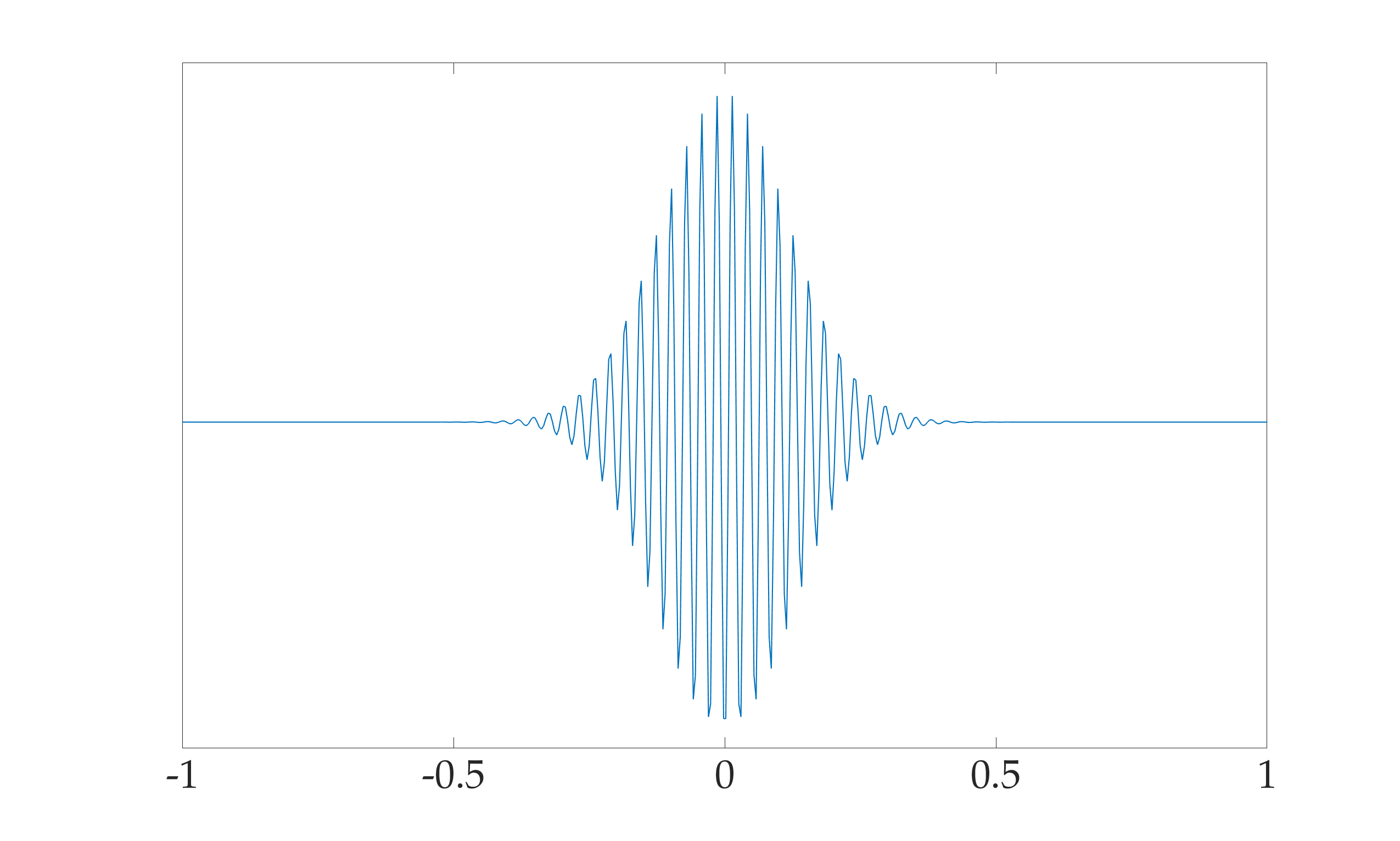
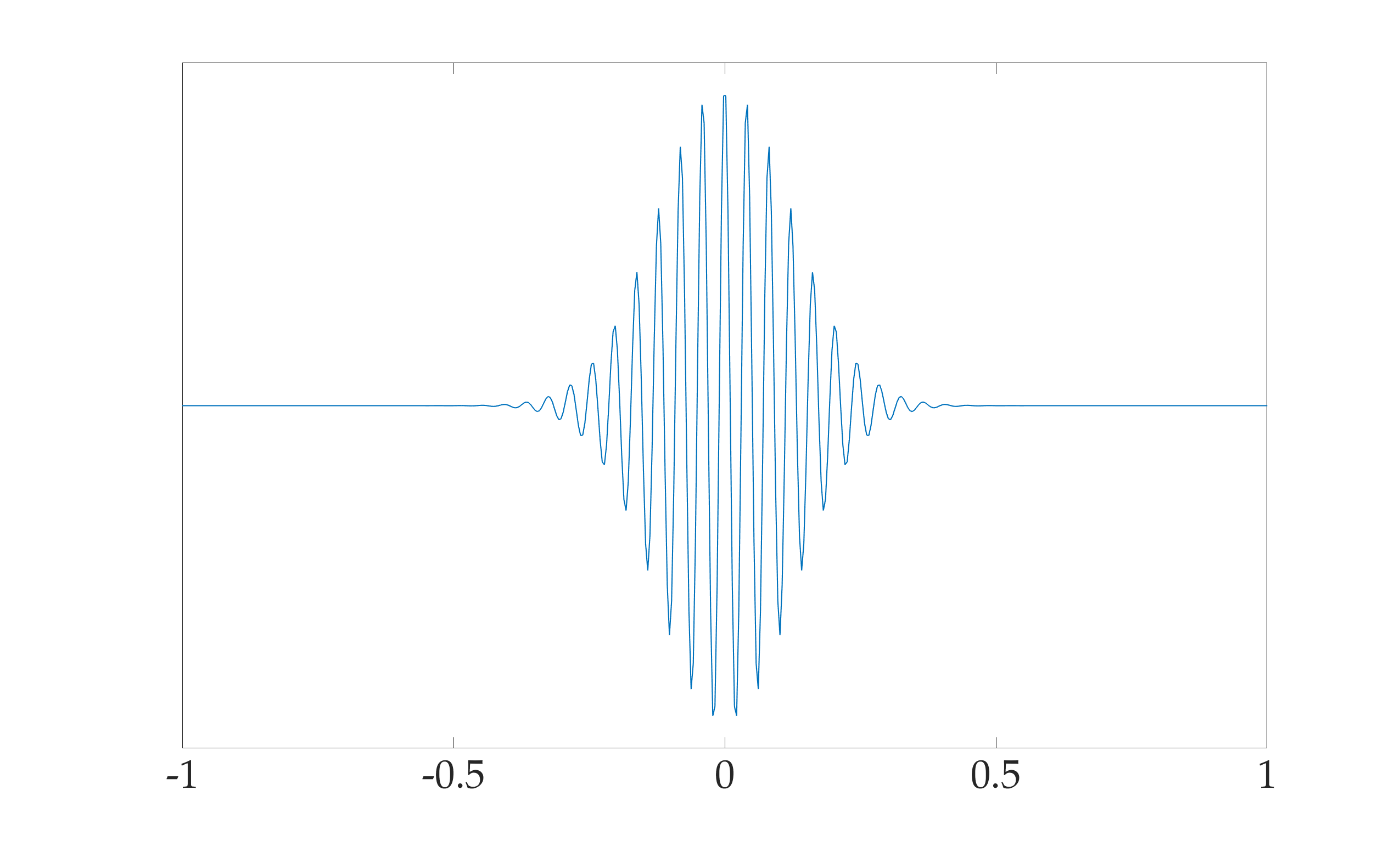
We present here some simulations showing the propagation of solutions to the fractional Schrödinger equation (1.1) corresponding to initial data in the form (1.2).

For the numerical resolution of the equation, we employed a uniform mesh in the space variable and a FE discretization of the fractional Laplacian, obtained following the methodology presented in [4]. Moreover, we used a Crank-Nicholson scheme in time, which is known to be stable for the Schrödinger equation (see, e.g., [1]). The initial data u0u_{0} has been chosen as

u0​(x)=e−γ2​(x−x0)2​ei​ξ0ε​x,\displaystyle u_{0}(x)=e^{-\frac{\gamma}{2}(x-x_{0})^{2}}e^{i\frac{\xi_{0}}{\varepsilon}x},

where the profile uin​(x)u_{\textrm{in}}(x) is given by a Gaussian with standard deviation measured in terms of the parameter γ\gamma, which is related to the mesh size hh. In particular we chose γ=h−0.9\gamma=h^{-0.9}. Finally, for the oscillations we considered frequencies ξ0=π2/16\xi_{0}=\pi^{2}/16 and ξ0=2​π2\xi_{0}=2\pi^{2}. We mention that this kind of approach is in many aspects analogous to what is done in [5, 24], where a similar analysis has been developed for the numerical finite difference solutions of one and two-dimensional waves, both with constant and variable coefficients.

In Figure 2, we show the plots for ξ0=2​π2\xi_{0}=2\pi^{2} and different values of s∈(0,1)s\in(0,1). The space domain has been chosen to be the interval (−1,1)(-1,1), while we considered a time interval of 55 seconds.

Refer to caption
(a) Initial data
Refer to caption
(b) s=0.1s=0.1
Refer to caption
(c) s=0.5s=0.5
Refer to caption
(d) s=0.9s=0.9
Figure 2: Propagation of the solution for ξ0=2​π2\xi_{0}=2\pi^{2} and different values of ss.

It is seen there that, for small values of ss, say s=0.1s=0.1, the solution remains concentrated along rays which propagate only in the vertical direction. In other words, there is no propagation in space and, as we mentioned before, this implies that it will not be possible to control these solutions, no matter how one places the controls. For s=0.5s=0.5, instead, the plots show that the solutions propagate along rays which reach the boundary of the space domain in finite time, and are reflected according to the laws of optics. This translates in the fact that, provided that the time is large enough, it will be possible to control these solutions, acting with a control distributed in a neighborhood ω\omega of the boundary. The case of high values of the power ss of the fractional Laplacian is the most puzzling one. For instance, for s=0.9s=0.9 our simulations seem to show a lost of concentration of the solution along the ray, while our theoretical results would suggest that this concentration is preserved. On the other hand, we believe that what the simulations are showing is not necessarily in contradiction with the theory. We are going to address this issue in more details a later time.
Refer to caption
(a) Initial data
Refer to caption
(b) s=0.1s=0.1
Refer to caption
(c) s=0.5s=0.5
Refer to caption
(d) s=0.9s=0.9
Figure 3: Propagation of the solution for ξ0=π2/16\xi_{0}=\pi^{2}/16 and different values of ss.

In Figure 3, the simulations have been run with an initial datum with frequency ξ0=π2/16\xi_{0}=\pi^{2}/16. The plots obtained show a behavior which is totally analogous with what observed in Figure 2:

  • ∙\bullet

    For s=0.1s=0.1, the solutions are once again concentrated along vertical rays, without propagation in time and, therefore, without possibility of being controlled.

  • ∙\bullet

    For s=0.5s=0.5, we have propagation with constant velocity, and the ray reaches the boundary in finite time.

  • ∙\bullet

    For s=0.9s=0.9 the chaotic comportment is still present.

Once again, the most surprising case is the last one, for s>0.5s>0.5, in which the simulations seem to display dispersive features. Nevertheless, as we mentioned before, we retain that this does not contradict the results of Section 4. In our opinion, this strange phenomenon appearing in the plot can be explained with the accumulation of higher order terms in the asymptotic expansion of zεz^{\,\varepsilon} which, combined with the small size of the space interval considered, enhance a chaotic behavior. This interpretation is supported by the fact that, as it is shown in Figure 4, enlarging the space domain up to (−6,6)(-6,6) seems to fix the problem and the localization of the solution along the rays appears once again.

Refer to caption
(a) ξ0=2​π2\xi_{0}=2\pi^{2}
Refer to caption
(b) ξ0=π2/16\xi_{0}=\pi^{2}/16
Figure 4: Propagation of the solution for s=0.9s=0.9 on the space interval (−6,6)(-6,6).

7 Conclusions and final remarks

In this article, we provided an explicit construction of a WKB ansatz for analyzing the propagation properties for a one-dimensional non-local Schrödigner equation involving the fractional Laplacian. In this way, we have been able to show that the solutions to the model that we considered are localized along the rays of geometric optics. In particular we proved that, the same as in the local case, the energy outside of a neighborhood of a ray is arbitrarily small. This fact can then be exploited for the study of controllability properties, in terms of the classical Geometric Control Condition.

To the best of our knowledge, this kind of analysis had not been developed yet in a non-local setting and this constitutes the main contribution of our work. Nevertheless, we must mention that our approach is asymptotically correct though far from being optimal.

Actually, it is commonly known that WKB is not the best technique for treating asymptotic analysis for wave-like PDEs. This because WKB solutions are usually subjected to caustic formation, which occurs at those points where the characteristic flow Φt\Phi_{t} associated to the equation ceases to be a diffeomorphism. Depending on the model analyzed, this may happen in a finite time TT, which might even be very small.

In general, this breakdown occurs when the density of rays becomes infinite. In that case, geometric optics incorrectly predicts that the amplitude of the solution is infinite. These problems are clearly not present in the exact solution of the model, but are merely an artifact of the WKB ansatz. Caustics, therefore, indicate the appearance of new ε\varepsilon-oscillatory scales, which are not captured by the simple oscillatory ansatz.

The consideration of these difficulties led to the development of the theory of other techniques related to micro-local analysis and propagation of singularities, such as Fourier integral operators, Gaussian beams or a Wigner transformation approach.

In particular, Gaussian beams is a high frequency asymptotic model which is closely related to geometrical optics. The quasi-solution are still assumed to be in the form

zε=a​eiε​ϕ,\displaystyle z^{\,\varepsilon}=ae^{\frac{i}{\varepsilon}\phi},

but unlike the WKB approach, in this case the phase is complex-valued. The main advantage of this is that there is no breakdown at caustics, thus providing an approximation which remains valid globally in time.

On the other hand, in the case of equation (1.1) considered in this paper, the choice of a complex-valued phase yields to technical difficulties at the moment of identifying the ansatz, which a the present stage we are not able to overcome. For this reason, we do not yet know how to develop a Guassian beam analysis for the solutions of our model.

We would like to stress that, for the specific case of (1.1), we do not face the problem of caustics formation, since the Hamiltonian system (2.1) admits a solution which is global in time. Nevertheless, this may not remain true when considering more general problems, for instance multi-dimensional or one with variable coefficients. For this reason, we believe that a different approach based on the aforementioned techniques should be developed in order to have a complete exhaustive understanding of the phenomena that we addressed in this paper.

8 Acknowledgements

This project has received funding from the European Research Council (ERC) under the European Union’s Horizon 2020 research and innovation programme (grant agreement No. 694126-DyCon). The work of the first was partially supported by the Grants MTM2014-52347 and MTM2017-92996 of MINECO (Spain) and by the Grant FA9550-18-1-0242 of AFOSR.

The authors wish to acknowledge Enrique Zuazua (Autonomous University of Madrid, DeustoTech and University of Deusto - Bilbao, and University Pierre and Marie Curie - Paris) for having suggested the topic of this research and for interesting discussions. A special thank goes to Aurora Marica (Polytechnic University of Bucharest) for her help for obtaining the simulations presented in this work. The second author (AA) thanks DeustoTech and the University of Deusto for hosting him in during summer of 2017, where part of this work was performed.

References

  • [1] Askar, A., and Cakmak, A. S. Explicit integration method for the time-dependent Schrodinger equation for collision problems. J. Chem. Phys. 68, 6 (1978), 2794–2798.
  • [2] Bardos, C., Lebeau, G., and Rauch, J. Sharp sufficient conditions for the observation, control, and stabilization of waves from the boundary. SIAM J. Control Optim. 30, 5 (1992), 1024–1065.
  • [3] Biccari, U. Internal control for non-local Schrödinger and wave equations involving the fractional Laplace operator. Preprint - arXiv:1411.7800 (2018).
  • [4] Biccari, U., and Hernández-Santamaría, V. Controllability of a one-dimensional fractional heat equation: theoretical and numerical aspects. IMA. J. Math. Control. I., doi:10.1093/imamci/dny025 (2018).
  • [5] Biccari, U., Marica, A., and Zuazua, E. Propagation of one and two-dimensional discrete waves under finite difference approximation. arXiv preprint arXiv:1806.09313 (2018).
  • [6] Biccari, U., Warma, M., and Zuazua, E. Local elliptic regularity for the Dirichlet fractional Laplacian. Adv. Nonlin. Stud. 17, 2 (2017), 387–409.
  • [7] Brillouin, L. La mécanique ondulatoire de Schrödinger; une méthode générale de résolution par approximations successives. Compt. Rend. Hebd. Seances Acad. Sci. 183 (1926), 24–26.
  • [8] Burq, N., and Gérard, P. Condition nécessaire et suffisante pour la contrôlabilité exacte des ondes. C.R. Acad. Sci. Sér. I Math. 325, 7 (1997), 749–752.
  • [9] Cazenave, T. Semilinear schrödinger equations, vol. 10. American Mathematical Soc., 2003.
  • [10] Červenỳ, V., Popov, M. M., and Pšenčík, I. Computation of wave fields in inhomogeneous media - Gaussian beam approach. Geophysics 70, 1 (1982), 109–128.
  • [11] Di Nezza, E., Palatucci, G., and Valdinoci, E. Hitchhikerʼs guide to the fractional Sobolev spaces. Bull. Sci. Math. 136, 5 (2012), 521–573.
  • [12] Hill, N. R. Prestack Gaussian-beam depth migration. Geophysics 66, 4 (2001), 1240–1250.
  • [13] Hörmander, L. The analysis of linear partial differential operators. I. Distribution theory and Fourier analysis. Springer Verlag, Berlin, 1990.
  • [14] Jumarie, G. Modified Riemann-Liouville derivative and fractional Taylor series of nondifferentiable functions further results. Comput. Math. Appl. 51, 9-10 (2006), 1367–1376.
  • [15] Kramers, H. A. Wellenmechanik und halbzahlige Quantisierung. Zeitschrift für Physik A Hadrons and Nuclei 39, 10 (1926), 828–840.
  • [16] Laskin, N. Fractional quantum mechanics. Phys. Rev. E 62, 3 (2000), 3135.
  • [17] Laskin, N. Fractional quantum mechanics and Lévy path integrals. Phys. Letters A 268, 4 (2000), 298–305.
  • [18] Laskin, N. Fractional Schrödinger equation. Phys. Rev. E 66, 5 (2002), 056108.
  • [19] Liu, H., and Ralston, J. Recovery of high frequency wave fields for the acoustic wave equation. Multis. Model. Simul. 8, 2 (2009), 428–444.
  • [20] Liu, H., and Ralston, J. Recovery of high frequency wave fields from phase space-based measurements. Multis. Model. Simul. 8, 2 (2010), 622–644.
  • [21] Liu, H., Runborg, O., and Tanushev, N. Error estimates for Gaussian beam superpositions. Math. Comput. 82, 282 (2013), 919–952.
  • [22] Liu, H., Runborg, O., and Tanushev, N. M. Sobolev and max norm error estimates for Gaussian beam superpositions. arXiv preprint arXiv:1510.09120 (2015).
  • [23] Longhi, S. Fractional Schrödinger equation in optics. Optics letters 40, 6 (2015), 1117–1120.
  • [24] Marica, A., and Zuazua, E. Propagation of 1D waves in regular discrete heterogeneous media: a Wigner measure approach. Found. Comput. Math. 15, 6 (2015), 1571–1636.
  • [25] Metzler, R., and Klafter, J. The random walk’s guide to anomalous diffusion: a fractional dynamics approach. Physics reports 339, 1 (2000), 1–77.
  • [26] Ralston, J. Gaussian beams and the propagation of singularities. Studies in partial differential equations 23 (1982), 206–248.
  • [27] Ros-Oton, X., and Serra, J. The Pohozaev identity for the fractional Laplacian. Arch. Ration. Mech. Anal. 213, 2 (2014), 587–628.
  • [28] Spigler, R., and Vianello, M. A survey on the Liouville-Green (WKB) approximation for linear difference equations of the second order. In Second International Conference on Difference Equations (1997), Gordon and Breach, pp. 567–577.
  • [29] Stickler, B. Potential condensed-matter realization of space-fractional quantum mechanics: The one-dimensional Lévy crystal. Phys. Rev. E 88, 1 (2013), 012120.
  • [30] Tanushev, N. M. Superpositions and higher order Gaussian beams. Comm. Math. Sc. 6, 2 (2008), 449–475.
  • [31] Tanushev, N. M., Qian, J., and Ralston, J. V. Mountain waves and Gaussian beams. Multiscale Modeling & Simulation 6, 2 (2007), 688–709.
  • [32] Trujillo, J., Rivero, M., and Bonilla, B. On a Riemann-Liouville generalized Taylor’s formula. J. Math. Anal. Appl. 231, 1 (1999), 255–265.
  • [33] Wentzel, G. Eine verallgemeinerung der quantenbedingungen für die zwecke der wellenmechanik. Zeitschrift für Physik A Hadrons and Nuclei 38, 6 (1926), 518–529.