Deep Domain Adaptation under Deep Label Scarcity
Abstract
The goal behind Domain Adaptation (DA) is to leverage the labeled examples from a source domain so as to infer an accurate model in a target domain where labels are not available or in scarce at the best. A state-of-the-art approach for the DA is due to [\citeauthoryearGanin et al.2016], known as DANN, where they attempt to induce a common representation of source and target domains via adversarial training. This approach requires a large number of labeled examples from the source domain to be able to infer a good model for the target domain. However, in many situations obtaining labels in the source domain is expensive which results in deteriorated performance of DANN and limits its applicability in such scenarios. In this paper, we propose a novel approach to overcome this limitation. In our work, we first establish that DANN reduces the original DA problem into a semi-supervised learning problem over the space of common representation. Next, we propose a learning approach, namely TransDANN, that amalgamates adversarial learning and transductive learning to mitigate the detrimental impact of limited source labels and yields improved performance. Experimental results (both on text and images) show a significant boost in the performance of TransDANN over DANN under such scenarios. We also provide theoretical justification for the performance boost.
Introduction
In many real life scenarios, label acquisition is a daunting task due to various limitations including cost, time, hazards, confidentiality, scale, etc. This limits the applicability of many successful machine learning and deep learning models which otherwise require a large number of labeled data. The field of domain adaptation (DA) aims at easing out learner’s job under such stress situations by allowing a transfer of learned models to other domain that faces label scarcity or absence. An example of such scenarios is commonly observed when immense amount of annotated labelled data [\citeauthoryearSun and Saenko2014, \citeauthoryearVazquez et al.2014] are created in the source domain whereas the target domain (often real world application domain) lacks annotation. The dissimilarity in marginal distribution of source domain and target domain data, called as covariate shift, is often significant and detrimental to the performance of source trained model on target data [\citeauthoryearShimodaira2000]. On the other hand, the dissimilarity of conditional distribution of source domain and target domain data, concept shift, can also impact performance of source trained model on target data despite absence of covariate shift [\citeauthoryearQuionero-Candela et al.2009]. For example, we might have an email spam filter trained from a large email collection received by a group of current users (the source domain) and wish to adapt it for a new user (the target domain) where we hardly have any email marked as spam by this new user [\citeauthoryearBen-David et al.2010a]. A similar situation arises during cold-start of an on-line recommender system when a new customer joins. In the email example, intuition suggests that we should be able to improve the performance of spam filter for the new user as long as we believe that users behave consistently in terms of labeling emails as spam or ham, denoted by . The challenge, however, is that each user receives a unique distribution of emails, say . The situation in the recommendation system example, on the other hand, could be little more complex. In this case, the behaviors of the users toward products need not be the same. That is may be different for different users. Furthermore, each user has a unique distribution, denoted by , from which he browses the products in the catalog. Therefore, transferring the learning may be bit hard. The email problem falls in a category of the DA problems where we say that covariate shift assumption holds. The recommendation engine problem, on the other hand, falls in the category of the DA problems where we say that both covariate shift as well as concept shift are present.
[\citeauthoryearBen-David et al.2010a] studied the class of DA problem where both covariate shift and concept shift are present but under the assumption that there exists a labeling rule, say , which works good for both the domains. In the very same setting, [\citeauthoryearGanin et al.2016] proposed Domain Adversarial Neural Networks (DANN) approach which extracts such an in deep learning framework. They achieve this objective by training the classifier to perform well on the source domain while minimizing the divergence between features extracted from the source versus target domains. For divergence minimization, they used domain adversarial training which leverages the target domain data without the need for their label. The deep learning framework enables to build the mapping between source domain and target domain through the domain classifier of the adversarial training.
As mentioned in [\citeauthoryearGanin et al.2016], DANN doesn’t require labeled examples from target domain but it requires a large number of labeled examples from source domain in order to output a classifier that is reasonably close to . The performance of DANN gets adversely affected when the supply of source domain labelled examples are limited - a situation common in real life. This happens because the error bound given in [\citeauthoryearBen-David et al.2010a] becomes noisy when labels are less and DANN tries to minimize this bound.
In this paper, we propose a novel approach, called as TransDANN, by fusing transductive learning theory with adversarial domain adaptation which prevents DANN suffering from low performance during deep scarcity of source labels. TransDANN is inspired by an early work of [\citeauthoryearJoachims1999] on transductive learning. We argue that DANN attempts to reduce an original DA problem into a semi-supervised learning problem over the extracted common space of domain-invariant features. This enables one to employ semi-supervised learning techniques for performance boosting. Experimental results (both on text and images) confirm the superiority of TransDANN over DANN.
Prior Art
The survey articles [\citeauthoryearPatel et al.2015], [\citeauthoryearCsurka2017], [\citeauthoryearWang and Deng2018] provide a landscape of the DA problem area. Broadly speaking, DA approaches belong to two categories - (i) conservative and (ii) non-conservative. In a conservative approach, information contained in unlabeled examples from the target domain is not leveraged. Whereas, in a non-conservative approach, it is leverage. Theoretical analysis of the conservative approaches can be found in [\citeauthoryearBen-David et al.2006], [\citeauthoryearBlitzer et al.2007], [\citeauthoryearMansour, Mohri, and Rostamizadeh2009]. Among non-conservative approaches, one idea is to re-weight the source labeled examples so as to match the marginal distributions of both the domains. [\citeauthoryearBen-David et al.2010b] and [\citeauthoryearBen-David et al.2010a] provided sound theoretical analysis for non-conservative approaches and proved an inevitable bound on the error of the learned hypothesis for the target domain. Recent approaches for non-conservative DA are inspired by the recent progress in the areas of deep neural networks and deep generative models [\citeauthoryearGoodfellow et al.2014]. The prominent approach along these lines include [\citeauthoryearLong et al.2015], [\citeauthoryearGanin et al.2016], and [\citeauthoryearTzeng et al.2017]. The idea in [\citeauthoryearGanin et al.2016] is to project both source and target marginal distributions into a common feature space and encourage projected distributions to match. They used the idea of generative adversarial nets [\citeauthoryearGoodfellow et al.2014] for this purpose. Other recent works along similar lines include [\citeauthoryearSaito, Ushiku, and Harada2017] and [\citeauthoryearShu et al.2018]. The approach proposed in [\citeauthoryearShu et al.2018] tries to improve DANN under the scenario where clustering assumption holds true for the target domain. In the text domain, [\citeauthoryearLiu, Qiu, and Huang2017, \citeauthoryearChen and Cardie2018] used adversarial training to obtain better generalization through multitask setting where both source and target domain data is available.
To the best of our knowledge, there is no other work which addresses the issue of DANN’s performance under source label scarcity. Our work is the first one to identify and address this gap.
Background – DA Problem Setup
A domain is defined as a tuple , where denotes the feature space, denotes the label space, and denotes the joint probability distribution function over the space .
In a typical DA problem setup, we are given a source domain and a target domain . The Bayes theorem allows us to write the density functions of the source and the target distributions as follows: 11 1 We use symbol to denote a distribution function and to denote the corresponding density function. . The density functions and are typically referred to as conditionals, whereas the functions and are referred to as marginals. In this paper, we assume . However, our results are applicable as long as and is any other label space which can be handled by deep neural networks.
The goal of any DA problem is to predict the label for any given target sample drawn from . The assumption is that both and are unknown to the learner. The only information available with the learner at the time of training is labeled examples (say ) from the source domain and unlabeled examples from the target domain, say . We denote these training data by , and , respectively.
Most of the DA work hinges around the assumption of and this setting is known as homogeneous DA [\citeauthoryearWang and Deng2018]. For the binary classification problem in this setting, [\citeauthoryearBen-David et al.2010a] gave a result (stated below) that relates the accuracy of any labeling function (aka hypothesis) on the source domain with the accuracy of the same hypothesis on the target domain.
Theorem 1 ([\citeauthoryearBen-David et al.2010a])
Let be a hypothesis space of VC dimension , then for any , with probability (over the choice of samples), for every :
where, error and are defined as the expected loss for the hypothesis with respect to the source and the target domain’s conditional distribution, respectively. That is, . The quantity denotes the distance between the distributions and and it accounts for the gap between and arising due to the discrepancy between and . This quantity is given by the following expression: where, . The constitutes the space of hypotheses which are pairwise symmetric difference of any two hypotheses from . By looking at , we can say that distance between the marginals of the source domain and the target domain can be calculated by identifying the best domain classifier which classifies the unlabeled examples from the source domain and the target domain. The exact same idea was exploited by [\citeauthoryearGanin et al.2016]. The last term is given by .
Following theorem is a refined version of Theorem 1 for the scenario when one has an empirical estimate of the quantity (and thereby, an empirical estimate ). This empirical estimate can be computed by having access to say unlabeled examples and drawn from and , respectively.
Theorem 2 ([\citeauthoryearBen-David et al.2010a])
This theorem offers the following insight. In order to find a good hypothesis for the target domain, one should aim to find a hypothesis space that not only contains a good hypothesis for the source domain, but also the best domain classifier in the space is as poor as possible.
Domain Adversarial Neural Networks (DANN)
Motivated by the above insights, [\citeauthoryearGanin et al.2016] proposed a novel feedforward neural network architecture, known as Domain Adversarial Neural Networks (DANN).
The DANN architecture starts with a mapping, , called as feature map, parameterized by the parameter . This feature map essentially projects any given unlabeled (source or target) example into a -dimensional Euclidean feature space. These feature vectors are then mapped to the class label (more generally, ) by means of another mapping, , called as label predictor. Lastly, the same feature vector is mapped to the domain label by means of the mapping, , known as domain classifier. The respective parameters of the label predictor and domain classifier are denoted by and , respectively. The hypothesis space for this network becomes the composition of and , given by , and the symmetric difference space becomes .
The training of DANN is very interesting. Note, the parameter is common to both hypothesis space as well as the symmetric difference hypothesis space . It is this parameter which on the one hand (along with the parameters ) helps tuning so as to include a hypothesis of low source domain error (first term in Equation (1)). While, on the other hand, it helps (along with the parameters ) adjusting the space so as the best domain classifying hypothesis becomes as poor as possible (last two terms in Equation (1)). This is achieved by finding the saddle point of the following loss function:
| (1) |
where, , , is a hyper-parameter, and is a cross-entropy loss function. The labels and represent the labels to identify the domain (source being and target being ) of any training example . The training of DANN proceeds in iterations where the aim is to find the saddle point of defined as below.
| (2) | |||||
| (3) |
The training of DANN is known to require a large amount of labeled examples from the source domain and a large amount of unlabeled examples from the target domain. Our proposed approach improves upon its training under the realistic setting when labeled examples in the source domain are few in numbers.
The Problem of Label Scarcity
Our initial experiments suggest (see Figure 1) that as we shrink the supply of labeled examples during DANN training, the resulting hypothesis of DANN deteriorates. In this figure, we have shown the performance of 6 different (source,target) domain pairs from Amazon product review dataset. For each pair, we have compared the performance of DANN output as we reduce the supply of labeled examples from 100% to 80%. The reasons behind such a behavior could be as follows. Given that DANN aims to minimize the error bound of Theorem 2, the estimate of the first term in this bound becomes noisy under label scarcity. This motivates us to revisit this problem and investigate whether one can improve the DANN training so as to handle label scarcity.
The key contribution of this paper lies in improving the DANN training so as to handle the deep label scarcity in the source domain. Our idea is based on the two key observations.
- 1.
The training of DANN with a large amount of unlabeled examples (both source and target domain) reduces the original DA problem into a semi-supervised learning problem over the single domain of common feature space.
- 2.
The resulting semi-supervised learning problem can be tackled in a way similar to the transductive learning problem handled in [\citeauthoryearJoachims1999].
Reduction to Semi-Supervised Learning Problem
Recall, that the marginal distributions and when pushed onto the feature space under the map obtained by training a DANN would be nearly identical. We denote such an induced marginal distribution in the feature space by and its density by . Under covariate shift assumption [\citeauthoryearShimodaira2000], one has . Thus, under the covariate shift assumption, one can use the output feature map of DANN to transform both source and target spaces and into the feature space where the problem now sounds more like a semi-supervised learning problem having few labeled examples and a large number of unlabeled examples. The labels of the examples in this feature space can be assumed to be sampled from some underlying distribution, say , and the feature vectors themselves can be assumed to be sampled from the common induced distribution . Any parameterized label classifier defined on this feature space can be combined with the feature map to render a classifier for the source or target domain. That is, .
Training a classifier in this feature space, thus, becomes a semi-supervised learning problem in its own. DANN outputs one such classifier given by . Any improvement on top of this classifier would indeed improve the accuracy of the target domain classifier as well. Therefore, we propose to invoke the approach of semi-supervised learning to offer a classifier that is better than what is DANN offers, especially when source labels are in scarcity.
Transductive Learning to Tackle Label Scarcity
Let be some domain. We need not confuse this with source (or target) domain being discussed so far. Suppose, a learner has access to labeled examples, , drawn independently from the distribution . The learner also has access to a large number of unlabeled examples drawn from the corresponding marginal distribution . The goal of the learner is to pick a hypothesis from the space so as to predict the labels of the examples in the set as accurately as possible.
For this kind of problems, [\citeauthoryearJoachims1999] proposed Transductive SVM approach where the idea is to minimize an appropriate loss function so as to find the joint optimal values for the model parameters as well as the labels for the unlabeled examples . Inspired by this, we first reduce the given DA problem into a semi-supervised learning problem over the common domain (feature space ) and subsequently improve the task classifier in a similar way. The net effect is that resulting classifier outperforms the classifier obtained by training the DANN.
TransDANN – The Proposed Approach
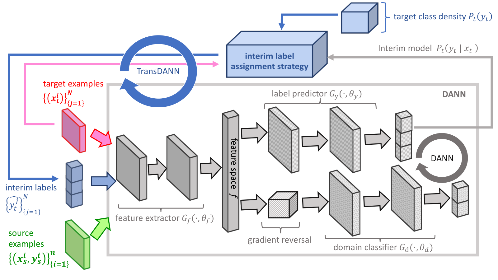
In this section, we give details of our proposed modified training approach for DANN. We call this approach as Transductive training of Deep Domain Neural Network (TransDANN). Figure 2 depicts the idea behind TransDANN approach.
In TransDANN approach, we being by defining the following alternative loss function called as TransDANN loss function.
| (4) |
where is a cross-entropy loss function and are the importance weights. This loss function has flavor of both DANN loss function (given by Equation (1)) and the transductive learning loss function (given in [\citeauthoryearJoachims1999]). The idea behind this loss function is to include the labels for the unlabeled examples (from the target domain) also as decision variables. As part of TransDANN training, we solve the following saddle point problem:
| (5) | |||
| (6) |
Observe, the first optimization problem (5) is a combinatorial optimization problem. Therefore, unlike DANN, the overall saddle point problem also becomes a combinatorial optimization problem.
Our proposed method to solve this saddle point problem is presented in the form of Algorithm 1 and it works as follows. It starts with a small number of labeled examples from the source domain and and a large number of unlabeled examples from the target domain. As a cold start, the method temporarily ignores the variables (and hence the second term in the Equation (4)). Instead, it trains a vanilla DANN on the given data so as to acquire an initial assignment of the -parameters, given by . Next, there is a loop which alternates between variables and so as to improve them in lieu of the sub-problems (5) – (6). That means, in one step (Step 1), it clamps the current assignment of the labels and improves upon the parameters in their local vicinity. In the subsequent step (Step 1), it clamps to their present values and revises the labels so as to reduce the loss. We call these revised labels as interim labels and denote them by .
In this alternation strategy, when improving upon the parameters locally, we follow a DANN like strategy because the second term of the TransDANN loss function is a constant. On the other hand, when improving upon the parameters , we need to solve the sub-problem (5) clamping the variables to their current values. Because this sub-problem (5) is a combinatorial optimization problem (due to the presence of ), we advocate the use of a local search strategy for this sub-problem. By local search strategy, we mean that we greedily revise the current assignment of the labels for so as to reduce the overall value of the loss function (4). In the next section, we describe one such strategy to assign interim labels.
In Algorithm 1, as iterations proceed, we slowly increase the importance weight until it hits the user specified upper bound . The value of dictates how much importance we wish to give to the semi-supervised part. Finally, suppose Algorithm 1 is given access to a validation set – a small labeled set from the target domain. In this situation, it compares the performance of the cold start model (offered by vanilla DANN) with the TransDANN model obtained at the end of iterative loop 7–12. The algorithm outputs a better of these two models, denoted by .
Interim Label Assignment Strategy
As far as the revision of the labels is concerned in Algorithm 1, there could be many strategies but we opt the following strategy which we call as matching the class distribution strategy. The idea behind this strategy is to assign the labels to the target domain examples in a way that these labels are in sync with the current label prediction model, call it , as much as possible, and at the same time, the distribution of the labels across the classes adhere to some apriori given numbers , where . The class densities are assumed to be either known or equal to which can be estimated from the source labeled examples. The reason being that throughout the TransDANN, induced marginals in the feature space remain the same and the label predictor also remains the common between source and target domains. Therefore, all the times.
For the general scenario of , this strategy is given in the form of Algorithm 2. This algorithm works as follows. First, we assign each example to the best class as per the supplied label prediction model . Next, we pick some class which has the surplus number of examples relative to its target . Among all the examples assigned to this class , we identify the one which has the weakest membership score and move that example to some other class, say . The class is chosen such that it has a deficiency of examples relative to its target and moreover, the identified example has strongest membership score for this class as compared to other classes who also have a deficiency.
Theoretical Analysis of TransDANN
Theorem given below guarantees that under some mild conditions, model learned by the TransDANN is no inferior than DANN. The proof relies on a fact that DANN ignores the term while minimizing the error bound of Theorem 2.
Theorem 3
Proof : Recall, DANN essentially tries to minimize the error bound given in Theorem 2. However, it tries to minimize the sum of only first two terms in the error bound of Theorem 2 and ignores the last term by treating it as a constant. We would like to highlight that the term is defined as . In the case of DANN, the hypothesis space is controlled by both and parameters. However, in DANN’s training, the update of and is never influenced by . The reason behind this is also apparent – DANN assumes no supply of the labeled data from the target domain and hence it has no way to estimate with reasonable accuracy.
On the other hand, in TransDANN, we indirectly estimate the term by the inclusion of a term capturing the label classification loss in the target domain. This term, in conjunction with the label classification loss for the source domain, mimics . In order to calculate this term, we need labels for the target domain which we get from the interim label assignment layer in the TransDANN. In the initial iterations, these interim labels are not accurate and hence the estimation of is poor. However, as iterations progress, the interim labels for the target domain examples improves and so does the estimation of . This helps TransDANN get an improved lower error bound than what DANN would get. Also, for the above argument to hold, we need covariate shift assumption because in each iteration of the TransDANN, we estimate interim labels of the target domain by using the current model for the source label. If covariate shift assumption is not true then we can’t assume that the labels estimated by interim label assignment layer during TransDANN training would eventually be trustworthy to get a good estimate of .
Experimental setup
To conduct an extensive set of experiments across various domains, we choose Amazon review dataset – a popular dataset among multi-domain deep learning (DL) methods [\citeauthoryearWu and Huang2015, \citeauthoryearChen and Cardie2018, \citeauthoryearGanin et al.2016]. We also experiment with MNIST and MNIST-M [\citeauthoryearGanin et al.2016] datasets which are commonly used for DA tasks in computer vision.
Dataset
For DA on text experiments, we work with Amazon review dataset 22 2 https://www.cs.jhu.edu/?mdredze/ datasets/sentiment/. This dataset comprises of customer reviews (in the text form) for 14 different product-lines (aka domains) at Amazon including Books, DVDs, Music, etc. The labels correspond to the sentiments of the reviewers. We extracted sentences and their corresponding labels from the raw data provided by [\citeauthoryearBlitzer, Dredze, and Pereira2007]. We processed the sentences using Stanford tokenizer 33 3 http://nlp.stanford.edu/software/ tokenizer.shtml. For each domain, the data are partitioned randomly into training, development, and test sets in a ratio of 70%, 10%, 20%, respectively. For our experimentation, we selected only 10 of these domains and hence we have skipped the details of the 4 domains from this tables as well as subsequent results. The detailed statistics of this dataset is given in supplementary material. For DA on images, we experiment with MNIST dataset available [\citeauthoryearLeCun et al.1998] as source and MNIST-M, obtained from [\citeauthoryearGanin et al.2016], as target domains.
Baselines
Our proposed approach aims to improve the DANN performance for DA tasks. Therefore, we treat the performance of the DANN as a baseline for our experiments. In our experiments, for each source-target domain pair, a baseline DANN model is trained as suggested in [\citeauthoryearGanin et al.2016]. In addition, to get an idea of how good the DANN itself perform in the first place, we also train a target-only model. We train such a target-only model using only the task classifer part of DANN architecture with labeled examples only from the target domain.
To emulate the label scarcity, we restrict the supply of labeled data from the source domain. Under such label scarcity (LS) scenarios, the performance of DANN deteriorates as shown in Figure 1. Our proposed approach, TransDANN, aims to achieve better performance (target accuracy) than DANN, especially under the LS scenarios. For relative comparison, we train the models using both DANN as well as TransDANN approaches under different LS scenarios. For text domain experiments, we limited the supply of the source labeled data ranging from 100% to 80% in each of source-target domain pair. Similarly, the image experiments are carried over the number of examples ranging 10000 to 4000 in each of source-target pair, i.e., MNIST and MNIST-M dataset. We found that performance of DANN remains similar with any number of examples more than 10000. For MNIST, we keep target supply same as that of source. We found that these range of label examples are required for reasonably good deep feature extraction.
| Target | dvd | books | elect | baby | kit | music | sports | app | cam | health |
|---|---|---|---|---|---|---|---|---|---|---|
| Source | ||||||||||
| dvd | 75.0 | 74.2 | 77.0 | 75.8 | 79.1 | 62.5 | 82.6 | 71.5 | 55.3 | |
| books | 83.0 | 78.9 | 74.6 | 78.9 | 80.3 | 79.7 | 81.4 | 81.4 | 72.9 | |
| elect | 74.4 | 74.2 | 79.1 | 79.3 | 73.4 | 81.6 | 82.0 | 74.6 | 77.1 | |
| baby | 63.9 | 71.3 | 80.9 | 82.4 | 70.3 | 79.1 | 79.5 | 77.0 | 54.5 | |
| kit | 70.7 | 69.3 | 77.1 | 77.0 | 63.9 | 80.5 | 82.2 | 75.8 | 80.1 | |
| music | 80.5 | 78.9 | 75.4 | 74.2 | 74.8 | 79.5 | 80.3 | 79.9 | 74.2 | |
| sports | 72.1 | 69.7 | 80.7 | 82.2 | 85.4 | 74.2 | 85.4 | 82.2 | 81.4 | |
| app | 72.9 | 69.9 | 79.5 | 80.5 | 79.5 | 72.9 | 73.6 | 76.4 | 78.5 | |
| cam | 76.8 | 71.3 | 80.3 | 74.4 | 77.7 | 71.5 | 80.1 | 78.1 | 80.9 | |
| health | 70.3 | 71.9 | 82.2 | 83.0 | 81.4 | 77.3 | 80.7 | 84.6 | 80.8 | |
| T-O | 83.9 | 88.0 | 81.4 | 83.9 | 81.8 | 78.6 | 85.1 | 80.6 | 83.7 | 84.5 |

Architecture
The proposed TransDANN approach comprises two main pieces – (i) DANN, and (ii) Interim Label Assignment.
DANN consists of feature extractor, task classifier, and domain adaptation layer. Feature extractor for the text domain adaptation can be composed of neural sentence models such as recurrent neural networks [\citeauthoryearSutskever, Vinyals, and Le2014, \citeauthoryearChung et al.2014, \citeauthoryearLiu et al.2015], convolution networks [\citeauthoryearCollobert et al.2011, \citeauthoryearKalchbrenner, Grefenstette, and Blunsom2014], or recursive neural networks [\citeauthoryearSocher et al.2013]. Here, we adopt recurrent neural network with long short-term memory (LSTM) due to their superior performance in various NLP tasks [\citeauthoryearLiu et al.2016, \citeauthoryearLin et al.2017]. Specifically, we compose feature extractor with a bidirectional-LSTM and task classifier with a fully connected layer – both as per the configurations suggested in the previous work on text modeling [\citeauthoryearLiu, Qiu, and Huang2017, \citeauthoryearLin et al.2017]. Preprocessing and tokenization of the input sentences are carried out as suggested by the standard NLP text modeling methods [\citeauthoryearLiu, Qiu, and Huang2017]. The words embedding for all the models are initialized with the 300-dimensional GloVe vectors [\citeauthoryearPennington, Socher, and Manning2014]. Other parameters are initialized by randomly sampling from a uniform distribution in the range . For the domain adapter component, we stick to three fully connected layers () as suggested by [\citeauthoryearGanin et al.2016]. For the image experiment, we use small CNN architecture for feature extractor, and 2 layer domain adapter () exactly as in [\citeauthoryearGanin et al.2016] . We choose cross-entropy and logistic regression loss for task classification and domain adapter, respectively.
The Interim Label Assignment layer assigns the target labels based on Algorithm 2, which are then fed to the input.
Training Procedure
The training under TransDANN proceeds in cycles. In each cycle, all the training examples are used in batches. The first cycle is purely DANN training and the interim labels for target examples kick in from the second cycle on-wards. Since true target labels are not available, the first cycle is trained simply as vanilla DANN wherein, the input batches are composed of labeled source examples and unlabeled target examples. From the second cycle onwards, the input to the model consists of interim target labels in addition to the source labels along with source and target examples. The interim target labels are generated by Interim Target Label Assignment (ITA) layer in the beginning of each cycle (except for the first cycle). The ITA layer ingests the trained model of the previous cycle and target class distribution so as to compute the new interim target labels using Algorithm 2. These iterative cycles continue till the convergence of target label training accuracy.
The model is trained on 128 sized batches for text and 64 sized for image. Half of each batch is composed of samples from the source domain and the other half with samples from the target domain. In the very first cycle, where we train vanilla DANN, we increase the domain adaptation factor slowly during early stage of the training so as to suppress noisy labels inferred by the domain classifier.
Choosing meta-parameters
The TransDANN training requires choosing meta-parameters (, learning rate, momentum, network architecture) in an unsupervised manner. One can assess the performance of the whole system (including the effect of hyper-parameters) by observing the error on a held-out data from the source domain as well as the training error on domain classification. For most of the meta-parameters, we have followed the guidelines from [\citeauthoryearGanin et al.2016]. In general, we have observed good correspondence between the DA task performance and the performance on the held-out data from the source domain which is in congruence with [\citeauthoryearGanin et al.2016].
Evaluation Results and Analysis
On Review dataset: We describe the evaluation results on text data in the following. We first obtain the baseline and then evaluate performance of TransDANN for each source-target pair under varying levels of source labels supply (ranging from 100% to 80%). Table 2 summarizes the maximum % improvement (over varying levels of source labels supply) achieved by TransDANN over DANN. Note, the diagonal elements are blank because experiments are conducted only for source-target pairs where so as to capture the efficacy of the proposed approach for DA tasks. The supplementary material contains the actual accuracy numbers over which these maximum % improvements are calculated.
A few important observations can be made from the Table 2. First, it’s clear that TransDANN outperforms DANN in several cases (% cases) by a noticeable margin. Second, in cases where TransDANN performance is close or equal to DANN, we often found that the performance of the DANN on target-only task is either too bad or too good. When performance of the DANN itself is too bad on the target-only task, there could potentially be issues other than the label scarcity, for example, covariate shift may not be holding true. In such cases, we anyways can’t expect TransDANN to improve significantly over DANN. On the other hand, when performance of the DANN itself is too good on the target-only task, there is not much scope for the TransDANN to improve.
Overall, the accuracy improvement of TransDANN over DANN is found to be significant under the scenarios where performance of the DANN gets affected due to the reduced supply of the source labels while the assumption of covariate shift holds true. To support this argument, we depict the performance of TransDANN over DANN with varying levels of source label supply in Figure 3 (refer supplementary material for enlarged version).
On Image dataset: Figure 4 captures the performance of our DA approach on MNIST to MNIST-M. Similar as above, we observe that when source (MNIST) data supply is limited DANN’s performance deteriorates and TranDANN outperforms in most of the cases.
Overall, both image and text dataset evaluation validates that TransDANN outperforms DANN in LS scenarios.
Concluding Remarks
In this paper, we present a novel approach, called TransDANN, which fuses adversarial learning and transductive learning methods for improved DA performance. Our approach outperforms DANN – a state-of-the-art – especially in scenarios where supply of source label in limited. We have provided theoretical as well as experimental justification in support of the proposed approach. The paper unveils and establishes that adversarial learning in effect reduces any DA problem into a semi-supervised learning in a space of common representation. Moreover, it opens up several avenues for employing various suitable semi-supervised techniques with existing adversarial based DA methods.
References
- [\citeauthoryearBen-David et al.2006] Ben-David, S.; Blitzer, J.; Crammer, K.; and Pereira, F. 2006. Analysis of representations for domain adaptation. In Proceedings of the 19th International Conference on Neural Information Processing Systems, NIPS, 137–144.
- [\citeauthoryearBen-David et al.2010a] Ben-David, S.; Blitzer, J.; Crammer, K.; Kulesza, A.; Pereira, F.; and Vaughan, J. W. 2010a. A theory of learning from different domains. Machine Learning 79(1):151–175.
- [\citeauthoryearBen-David et al.2010b] Ben-David, S.; Lu, T.; Luu, T.; and Pal, D. 2010b. Impossibility theorems for domain adaptation. In Proceedings of the 13th International Conference on Artificial Intelligence and Statistics, AISTATS, 129–136.
- [\citeauthoryearBlitzer et al.2007] Blitzer, J.; Crammer, K.; Kulesza, A.; Pereira, F.; and Wortman, J. 2007. Learning bounds for domain adaptation. In Proceedings of the 20th International Conference on Neural Information Processing Systems, NIPS’07, 129–136.
- [\citeauthoryearBlitzer, Dredze, and Pereira2007] Blitzer, J.; Dredze, M.; and Pereira, F. 2007. Biographies, bollywood, boomboxes and blenders: Domain adaptation for sentiment classification. In Proceedings of the Annual Meeting of the Association for Computational Linguistics, ACL’07, 187–205.
- [\citeauthoryearChen and Cardie2018] Chen, X., and Cardie, C. 2018. Multinomial adversarial networks for multi-domain text classification. In Proceedings of the Conference of the North American Chapter of the Association for Computational Linguistics, NAACL’18, 1226–1240.
- [\citeauthoryearChung et al.2014] Chung, J.; Gulcehre, C.; Cho, K.; and Bengio, Y. 2014. Empirical evaluation of gated recurrent neural networks on sequence modeling. In arXiv preprint arXiv:1412.3555.
- [\citeauthoryearCollobert et al.2011] Collobert, R.; Weston, J.; Bottou, L.; Karlen, M.; Kavukcuoglu, K.; and Kuksa, P. 2011. Natural language processing (almost) from scratch. Journal of Machine Learning Research 12:2493–2537.
- [\citeauthoryearCsurka2017] Csurka, G. 2017. A Comprehensive Survey on Domain Adaptation for Visual Applications. Springer International Publishing. 1–35.
- [\citeauthoryearGanin et al.2016] Ganin, Y.; Ustinova, E.; Ajakan, H.; Germain, P.; Larochelle, H.; Laviolette, F.; Marchand, M.; and Lempitsky, V. S. 2016. Domain-adversarial training of neural networks. Journal of Machine Learning Research 17:1–35.
- [\citeauthoryearGoodfellow et al.2014] Goodfellow, I. J.; Pouget-Abadie, J.; Mirza, M.; Xu, B.; Warde-Farley, D.; Ozair, S.; Courville, A. C.; and Bengio, Y. 2014. Generative adversarial nets. In Proceedings of the 27th International Conference on Neural Information Processing Systems, NIPS’17, 2672–2680.
- [\citeauthoryearJoachims1999] Joachims, T. 1999. Transductive inference for text classification using support vector machines. In Proceedings of the 16th International Conference on Machine Learning, ICML’99, 200–209.
- [\citeauthoryearKalchbrenner, Grefenstette, and Blunsom2014] Kalchbrenner, N.; Grefenstette, E.; and Blunsom, P. 2014. A convolutional neural network for modelling sentences. In Proceedings of the Annual Meeting of the Association for Computational Linguistics, ACL’14.
- [\citeauthoryearLeCun et al.1998] LeCun, Y.; Bottou, L.; Bengio, Y.; and Haffner, P. 1998. Gradient- based learning applied to document recognition. In Proceedings of the IEEE, volume 86(11), 2278–2324.
- [\citeauthoryearLin et al.2017] Lin, Z.; Feng, M.; Santos, C. N. d.; Yu, M.; Xiang, B.; Zhou, B.; and Bengio, Y. 2017. A structured self-attentive sentence embedding. In arXiv preprint arXiv:1703.03130.
- [\citeauthoryearLiu et al.2015] Liu, P.; Qiu, X.; Chen, X.; Wu, S.; and Huang, X. 2015. Multi-timescale long short-term memory neural network for modelling sentences and documents. In Proceedings of the Conference on Empirical Methods in Natural Language Processing, EMNLP’15.
- [\citeauthoryearLiu et al.2016] Liu, P.; Qiu, X.; Chen, J.; and Huang, X. 2016. Deep fusion lstms for text semantic matching. In Proceedings of the Annual Meeting of the Association for Computational Linguistics, ACL’16.
- [\citeauthoryearLiu, Qiu, and Huang2017] Liu, P.; Qiu, X.; and Huang, X. 2017. Adversarial multi-task learning for text classification. In Proceedings of the Annual Meeting of the Association for Computational Linguistics, ACL’17, 1–10.
- [\citeauthoryearLong et al.2015] Long, M.; Cao, Y.; Wang, J.; and Jordan, M. I. 2015. Learning transferable features with deep adaptation networks. In Proceedings of the 32nd International Conference on International Conference on Machine Learning, ICML’15, 97–105.
- [\citeauthoryearMansour, Mohri, and Rostamizadeh2009] Mansour, Y.; Mohri, M.; and Rostamizadeh, A. 2009. Domain adaptation: Learning bounds and algorithms. In Proceedings of the 22nd Conference on Learning Theory, COLT’09.
- [\citeauthoryearPatel et al.2015] Patel, V. M.; Gopalan, R.; Li, R.; and Chellappa, R. 2015. Visual domain adaptation: A survey of recent advances. IEEE Signal Process. Mag. 32(3):53–69.
- [\citeauthoryearPennington, Socher, and Manning2014] Pennington, J.; Socher, R.; and Manning, C. D. 2014. Glove: Global vectors for word representation. In Proceedings of the Conference on Empirical Methods in Natural Language Processing, EMNLP’14, 1532–1543.
- [\citeauthoryearQuionero-Candela et al.2009] Quionero-Candela, J.; Sugiyama, M.; Schwaighofer, A.; and Lawrence, N. D. 2009. Dataset shift in machine learning. The MIT Press.
- [\citeauthoryearSaito, Ushiku, and Harada2017] Saito, K.; Ushiku, Y.; and Harada, T. 2017. Asymmetric tri-training for unsupervised domain adaptation. In Proceedings of the 6th International Conference on Learning Representations, ICLR’17, 2988–2997.
- [\citeauthoryearShimodaira2000] Shimodaira, H. 2000. Improving predictive inference under covariate shift by weighting the log-likelihood function. Journal of Statistical Planning and Inference 90(2):227 – 244.
- [\citeauthoryearShu et al.2018] Shu, R.; Bui, H. H.; Narui, H.; and Ermon, S. 2018. A DIRT-T approach to unsupervised domain adaptation. In Proceedings of the 34th International Conference on Machine Learning, ICML’18.
- [\citeauthoryearSocher et al.2013] Socher, R.; Perelygin, A.; Wu, J. Y.; Chuang, J.; Manning, C. D.; Y Ng, A.; and Potts, C. 2013. Recursive deep models for semantic compositionality over a sentiment treebank. In Proceedings of the Conference on Empirical Methods in Natural Language Processing, EMNLP’13.
- [\citeauthoryearSun and Saenko2014] Sun, B., and Saenko, K. 2014. From virtual to reality: Fast adaptation of virtual object detectors to real domains. In British Machine Vision Conference, BMVC’14.
- [\citeauthoryearSutskever, Vinyals, and Le2014] Sutskever, I.; Vinyals, O.; and Le, Q. V. 2014. Sequence to sequence learning with neural networks. In in Proceedings of the Conference on Neural Information Processing Systems, NIPS’14, 3104–3112.
- [\citeauthoryearTzeng et al.2017] Tzeng, E.; Hoffman, J.; Saenko, K.; and Darrell, T. 2017. Adversarial discriminative domain adaptation. In Proceedings of Conference on Computer Vision and Pattern Recognition, CVPR’17.
- [\citeauthoryearVazquez et al.2014] Vazquez, D.; Lopez, A. M.; Marin, J.; Ponsa, D.; and Geronimo, D. 2014. Virtual and real world adaptation for pedestrian detection. In IEEE transactions on pattern analysis and machine intelligence, volume 36(4), 797–809.
- [\citeauthoryearWang and Deng2018] Wang, M., and Deng, W. 2018. Deep visual domain adaptation: A survey. Neurocomputing 312:135 – 153.
- [\citeauthoryearWu and Huang2015] Wu, F., and Huang, Y. 2015. Collaborative multi-domain sentiment classification. In IEEE International Conference on Data Mining, ICDM’15, 459–468.
Appendix A Appendix
Summary Statistics of Amazon Review Dataset
Table 3 (in this supplementary document) provides a detailed summary of the Amazon review dataset that were used in our experiments.
| Dataset | Train | Dev. | Test | Unlab. | Avg.L. | Vocab |
|---|---|---|---|---|---|---|
| Books | 1400 | 200 | 400 | 2000 | 159 | 62k |
| Electronics (elec) | 1398 | 200 | 400 | 2000 | 101 | 30k |
| DVD | 1300 | 200 | 400 | 2000 | 173 | 69k |
| Kitchen (kit) | 1400 | 200 | 400 | 2000 | 89 | 28k |
| Apparel (app) | 1400 | 200 | 400 | 2000 | 57 | 21k |
| Camera (cam) | 1397 | 200 | 400 | 2000 | 130 | 26k |
| Health (heal) | 1400 | 200 | 400 | 2000 | 81 | 26k |
| Music | 1400 | 200 | 400 | 2000 | 136 | 60k |
| Baby | 1300 | 200 | 400 | 2000 | 104 | 26k |
| Sports | 1315 | 200 | 400 | 2000 | 94 | 30k |
Elaboration of Table 2
Table 2 in the main paper depicts the maximum % improvement in accuracy of TransDANN over DANN, where max is computed over varying amount of labeled data. In what follows, we have presented the corresponding actual accuracy numbers for both DANN and TransDANN (for varying levels of labeled data). In all these tables (Table 5 – 9 in this supplementary document), the rows correspond to the source domains and the columns correspond to the target domains.
| dvd | books | elect | baby | kit | music | sports | app | cam | health | |
|---|---|---|---|---|---|---|---|---|---|---|
| dvd | 77.1 | 73.9 | 76.6 | 76.2 | 79.3 | 71.1 | 83.5 | 71.5 | 56.8 | |
| books | 85.7 | 78.3 | 73.7 | 78.6 | 80.2 | 80.2 | 81.8 | 82.7 | 74.0 | |
| elect | 73.9 | 73.0 | 72.6 | 79.0 | 73.0 | 79.8 | 83.6 | 74.0 | 76.4 | |
| baby | 59.6 | 70.6 | 75.5 | 81.8 | 71.3 | 79.0 | 79.8 | 77.1 | 54.6 | |
| kit | 70.4 | 68.3 | 78.5 | 76.2 | 64.8 | 80.7 | 83.7 | 75.8 | 78.8 | |
| music | 81.4 | 77.4 | 74.0 | 75.1 | 76.2 | 79.6 | 80.3 | 80.2 | 74.9 | |
| sports | 75.0 | 72.0 | 80.1 | 81.9 | 84.3 | 74.9 | 86.1 | 82.6 | 82.6 | |
| app | 72.6 | 73.2 | 79.9 | 79.9 | 80.6 | 74.7 | 76.0 | 77.3 | 78.8 | |
| cam | 76.0 | 70.2 | 79.9 | 78.4 | 80.5 | 73.8 | 81.5 | 75.5 | 81.3 | |
| health | 72.1 | 71.8 | 82.6 | 82.7 | 82.9 | 77.8 | 80.9 | 84.4 | 80.4 |
| dvd | books | elect | baby | kit | music | sports | app | cam | health | |
|---|---|---|---|---|---|---|---|---|---|---|
| dvd | 75.0 | 74.2 | 77.0 | 75.8 | 79.1 | 62.5 | 82.6 | 71.5 | 55.3 | |
| books | 83.2 | 78.9 | 74.6 | 78.9 | 80.3 | 79.7 | 81.4 | 81.4 | 73.0 | |
| elect | 74.4 | 74.2 | 79.1 | 79.3 | 73.4 | 81.6 | 82.6 | 74.6 | 77.7 | |
| baby | 69.7 | 71.3 | 80.9 | 82.4 | 71.7 | 79.1 | 79.5 | 78.5 | 54.5 | |
| kit | 70.7 | 69.5 | 77.1 | 77.1 | 63.9 | 80.5 | 82.2 | 76.4 | 80.5 | |
| music | 80.5 | 78.9 | 75.4 | 74.2 | 74.8 | 79.5 | 80.3 | 79.9 | 74.2 | |
| sports | 72.1 | 69.7 | 80.9 | 82.2 | 85.4 | 74.2 | 85.4 | 82.2 | 81.4 | |
| app | 72.9 | 69.9 | 79.5 | 80.5 | 79.5 | 72.9 | 73.8 | 76.4 | 78.5 | |
| cam | 76.8 | 71.3 | 80.3 | 74.4 | 79.5 | 71.5 | 80.1 | 78.1 | 80.9 | |
| health | 70.3 | 71.9 | 82.2 | 83.0 | 81.4 | 77.3 | 80.7 | 84.6 | 80.9 |
| dvd | books | elect | baby | kit | music | sports | app | cam | health | |
| dvd | 75.5 | 67.5 | 76.7 | 76.0 | 78.8 | 73.5 | 82.7 | 70.2 | 56.2 | |
| books | 82.9 | 78.8 | 73.4 | 79.3 | 79.7 | 80.7 | 82.6 | 79.6 | 75.0 | |
| elect | 75.6 | 74.4 | 78.3 | 79.4 | 73.8 | 80.3 | 83.8 | 78.0 | 78.2 | |
| baby | 62.0 | 71.3 | 73.9 | 82.6 | 63.6 | 79.1 | 81.6 | 76.4 | 63.7 | |
| kit | 69.9 | 67.6 | 79.0 | 77.9 | 64.6 | 80.5 | 79.3 | 76.4 | 79.5 | |
| music | 81.3 | 78.0 | 72.7 | 74.9 | 73.4 | 79.8 | 79.2 | 79.4 | 73.2 | |
| sports | 73.6 | 72.9 | 80.1 | 81.6 | 85.4 | 74.7 | 84.9 | 54.6 | 81.1 | |
| app | 70.8 | 71.3 | 79.6 | 79.3 | 80.3 | 73.8 | 77.0 | 71.5 | 75.3 | |
| cam | 76.2 | 73.6 | 80.3 | 80.2 | 78.1 | 72.1 | 82.0 | 77.0 | 81.7 | |
| health | 71.2 | 73.0 | 80.3 | 82.6 | 83.3 | 77.7 | 79.7 | 84.7 | 79.1 |
| dvd | books | elect | baby | kit | music | sports | app | cam | health | |
| dvd | 77.0 | 69.3 | 76.4 | 75.6 | 77.0 | 73.8 | 82.2 | 64.6 | 58.8 | |
| books | 83.0 | 79.3 | 73.8 | 79.1 | 79.1 | 80.7 | 81.4 | 82.2 | 74.0 | |
| elect | 76.2 | 75.0 | 76.6 | 80.5 | 77.1 | 80.3 | 82.2 | 82.0 | 78.9 | |
| baby | 71.9 | 70.7 | 79.3 | 83.0 | 73.2 | 80.1 | 83.8 | 74.4 | 69.3 | |
| kit | 69.1 | 66.0 | 78.3 | 80.1 | 67.8 | 80.1 | 83.4 | 76.8 | 79.7 | |
| music | 80.7 | 77.0 | 71.7 | 73.6 | 75.4 | 81.4 | 78.3 | 78.1 | 72.5 | |
| sports | 74.6 | 73.2 | 81.2 | 82.4 | 84.8 | 75.2 | 84.6 | 80.7 | 80.9 | |
| app | 67.8 | 74.0 | 78.7 | 77.3 | 82.2 | 75.2 | 76.8 | 69.7 | 77.9 | |
| cam | 78.1 | 72.9 | 81.4 | 78.9 | 78.5 | 68.2 | 82.6 | 74.0 | 83.0 | |
| health | 69.9 | 73.2 | 78.9 | 82.8 | 84.0 | 77.5 | 80.7 | 85.9 | 77.1 |
| dvd | books | elect | baby | kit | music | sports | app | cam | health | |
| dvd | 76.7 | 68.4 | 75.7 | 76.2 | 75.2 | 66.7 | 79.6 | 68.9 | 59.2 | |
| books | 82.3 | 79.3 | 73.3 | 79.0 | 79.4 | 79.9 | 80.4 | 80.2 | 75.5 | |
| elect | 70.8 | 75.6 | 72.3 | 71.0 | 67.1 | 80.8 | 82.9 | 77.5 | 75.1 | |
| baby | 61.8 | 69.8 | 74.9 | 79.2 | 72.5 | 78.6 | 73.4 | 74.7 | 68.7 | |
| kit | 63.2 | 68.8 | 78.3 | 79.3 | 69.3 | 80.0 | 76.4 | 76.0 | 79.8 | |
| music | 82.7 | 78.3 | 73.6 | 74.2 | 74.2 | 81.1 | 79.7 | 78.9 | 73.0 | |
| sports | 71.9 | 70.6 | 80.6 | 78.7 | 82.7 | 74.6 | 84.2 | 75.3 | 80.6 | |
| app | 69.4 | 73.6 | 78.9 | 78.3 | 82.0 | 75.9 | 77.9 | 70.4 | 76.8 | |
| cam | 75.0 | 72.1 | 78.9 | 78.9 | 76.3 | 69.8 | 80.9 | 68.8 | 82.1 | |
| health | 71.0 | 74.0 | 81.2 | 80.6 | 83.1 | 78.3 | 78.4 | 84.6 | 78.2 |
| dvd | books | elect | baby | kit | music | sports | app | cam | health | |
|---|---|---|---|---|---|---|---|---|---|---|
| dvd | 78.3 | 72.1 | 72.5 | 76.6 | 77.7 | 72.5 | 78.3 | 66.2 | 61.3 | |
| books | 81.6 | 78.5 | 74.8 | 79.3 | 79.5 | 78.5 | 77.5 | 78.5 | 75.6 | |
| elect | 61.9 | 77.5 | 65.4 | 51.6 | 76.6 | 81.2 | 81.8 | 75.0 | 68.2 | |
| baby | NaN | 70.7 | 71.5 | 80.5 | 70.7 | 80.1 | 57.0 | 76.0 | 54.5 | |
| kit | 50.6 | 68.2 | 79.1 | 79.7 | 71.7 | 81.1 | 78.1 | 76.8 | 80.5 | |
| music | 82.0 | 80.1 | 76.4 | 74.0 | 76.6 | 82.0 | 79.5 | 80.7 | 74.2 | |
| sports | 71.5 | 70.1 | 79.3 | 77.3 | 80.1 | 73.2 | 84.4 | 77.1 | 80.1 | |
| app | 73.0 | 72.9 | 78.5 | 78.9 | 82.0 | 74.2 | 76.8 | 69.7 | 75.8 | |
| cam | 74.8 | 72.3 | 79.3 | 78.7 | 77.0 | 66.8 | 77.3 | 57.0 | 79.9 | |
| health | 70.3 | 74.0 | 80.3 | 79.5 | 84.0 | 77.9 | 78.7 | 85.7 | 77.0 |