跳到论文正文
W Papers独立论文阅读器 arXiv:1809.08055 论文正文 计算阅读时间 · 0%
引用这篇论文根据当前论文元数据生成,正式投稿前建议核对。


License: arXiv.org perpetual non-exclusive license
arXiv:1809.08055v4 [cs.DS] 06 Jan 2019

Compressed Sensing with Adversarial Sparse Noise via L1 Regression

Sushrut Karmalkar Email: sushrutk@cs.utexas.edu Affiliation: UT Austin    Eric Price Email: ecprice@cs.utexas.edu Affiliation: UT Austin
Abstract

We present a simple and effective algorithm for the problem of sparse robust linear regression. In this problem, one would like to estimate a sparse vector w∗∈ℝnw^{*}\in\mathbb{R}^{n} from linear measurements corrupted by sparse noise that can arbitrarily change an adversarially chosen η\eta fraction of measured responses yy, as well as introduce bounded norm noise to the responses.

For Gaussian measurements, we show that a simple algorithm based on L1 regression can successfully estimate w∗w^{*} for any η<η0≈0.239\eta<\eta_{0}\approx 0.239, and that this threshold is tight for the algorithm. The number of measurements required by the algorithm is O⁡(k​log⁡nk)O(k\log\frac{n}{k}) for kk-sparse estimation, which is within constant factors of the number needed without any sparse noise.

Of the three properties we show—the ability to estimate sparse, as well as dense, w∗w^{*}; the tolerance of a large constant fraction of outliers; and tolerance of adversarial rather than distributional (e.g., Gaussian) dense noise—to the best of our knowledge, no previous result achieved more than two.

1 Introduction

Linear regression is the problem of estimating a signal vector from noisy linear measurements. It is a classic problem with applications in almost every field of science. In recent decades, it has also become popular to impose a sparsity constraint on the signal vector. This is known as “sparse recovery” or “compressed sensing”, and (when the assumption holds) can lead to significant savings in the number of measurements required for accurate estimation.

A well-known problem with the most standard approaches to linear regression and compressed sensing is that they are not robust to outliers in the data. If even a single data point (xi,yi)(x_{i},y_{i}) is perturbed arbitrarily, the estimates given by the algorithms can also be perturbed arbitrarily far. Addressing this for linear regression is one of the primary focuses of the field of robust statistics [Hub11]. Unfortunately, while the problem is clear, the solution is not—no fully satisfactory robust algorithms exist, particularly for high-dimensional data.

In this paper, we consider the model of robustness in which only the responses yiy_{i}, not the features xix_{i}, are corrupted by outliers. In this model, if the features xix_{i} are i.i.d. normal, we show that the classic algorithm of L1 minimization performs well and has fairly high robustness, for both dense and sparse linear regression. In particular, we consider the observation model

y=X​w∗+ζ+d\displaystyle y=Xw^{*}+\zeta+d (1)

where X∈ℝm×nX\in\mathbb{R}^{m\times n} is the observation matrix, w∗∈ℝnw^{*}\in\mathbb{R}^{n} is the kk-sparse signal, ζ∈ℝm\zeta\in\mathbb{R}^{m} is an η​m\eta m-sparse noise vector, and d∈ℝmd\in\mathbb{R}^{m} is a (possibly dense) noise vector. We will focus on the case of XX having i.i.d. N⁡(0,1)N(0,1) entries, but the core lemmas and techniques can apply somewhat more generally.

Without adversarial corruptions—i.e. if η=0\eta=0 so ζ=0\zeta=0—this would be the compressed sensing problem. The most standard solution for compressed sensing [CRT06] is L1 minimization: if m>Θ⁡(k​log⁡nk)m>\Theta(k\log\frac{n}{k}) then with high probability

w^:=arg​min‖y−Xw‖2≤σ⁡‖w‖1\widehat{w}:=\argmin_{\|y-Xw\|_{2}\leq\sigma}\|w\|_{1}

for any σ>‖d‖2\sigma>\|d\|_{2} will satisfy ‖w^−w∗‖2≤O⁡(σ/m)\|\widehat{w}-w^{*}\|_{2}\leq O(\sigma/\sqrt{m}). Unfortunately, this algorithm is not robust to sparse noise of large magnitude: a single faulty measurement yiy_{i} can make the (‖y−X​w‖2≤σ)(\|y-Xw\|_{2}\leq\sigma) ball infeasible.

To make the algorithm robust to sparse measurement noise, a natural approach is to replace the (non-robust) ℓ2\ell_{2} norm with the (robust) ℓ1\ell_{1} norm, as well as to swap the objective and the constraint. This ensures that the constrained parameter does not involve outliers. In this paper we show that this approach works, i.e., we show that

w^:=arg​min‖w‖1≤λ⁡‖y−Xw‖1\displaystyle\widehat{w}:=\argmin_{\|w\|_{1}\leq\lambda}\|y-Xw\|_{1} (2)

is a robust estimator for w∗w^{*}. In the following theorem, we show that (2) is robust to any fraction of corruptions η\eta less than η0:=2​(1−Φ⁡(2​log⁡2))≈0.239\eta_{0}:=2\left(1-\Phi(\sqrt{2\log 2})\right)\approx 0.239, where Φ:ℝ→[0,1]\Phi:\mathbb{R}\to[0,1] is the standard normal CDF. If λ=‖w∗‖1\lambda=\|w^{*}\|_{1}, the reconstruction error is O⁡(‖d‖1/m)O(\|d\|_{1}/m); for larger λ\lambda, it additionally grows with λ−‖w∗‖1\lambda-\|w^{*}\|_{1}:

Theorem 1.1 (Sparse Case).

Let η<η0−ϵ\eta<\eta_{0}-\epsilon where ϵ>0\epsilon>0, and let X∈ℝm×nX\in\mathbb{R}^{m\times n} have i.i.d. N⁡(0,1)N(0,1) entries with m>C​α2ϵ2​k​log⁡(e​nα2​ϵ​k)m>C\frac{\alpha^{2}}{\epsilon^{2}}k\log(\frac{en}{\alpha^{2}\epsilon k}) for some large enough constant CC and parameter α≥2ϵ\alpha\geq\frac{2}{\epsilon}. Then with probability 1−e−Ω⁡(ϵ2​m)1-e^{-\Omega(\epsilon^{2}m)} the matrix XX will have the following property: for any y=X​w∗+d+ζy=Xw^{*}+d+\zeta with ‖w∗‖0≤k\|w^{*}\|_{0}\leq k and ‖ζ‖0≤η​m\|\zeta\|_{0}\leq\eta m,

w^:=arg​min‖w‖1≤λ⁡‖y−Xw‖1\widehat{w}:=\argmin_{\|w\|_{1}\leq\lambda}\|y-Xw\|_{1}

for λ≥‖w∗‖1\lambda\geq\|w^{*}\|_{1} satisfies

‖w∗−w^‖2≤O⁡(1ϵ−1α​(1m​‖d‖1)+λ−‖w∗‖1α​k).\|w^{*}-\widehat{w}\|_{2}\leq O\left(\frac{1}{\epsilon-\frac{1}{\alpha}}\left(\frac{1}{m}\|d\|_{1}\right)+\frac{\lambda-\|w^{*}\|_{1}}{\alpha\sqrt{k}}\right).

In the case where w∗w^{*} is not sparse, the reconstruction error is shown to be O⁡(‖d‖1/m)O(\|d\|_{1}/m) in O⁡(n)O(n) samples using essentially the same proof.

Theorem 1.2 (Dense Case).

Let η<η0−ϵ\eta<\eta_{0}-\epsilon where ϵ>0\epsilon>0, and let X∈ℝm×nX\in\mathbb{R}^{m\times n} have i.i.d. N⁡(0,1)N(0,1) entries with m>C​nϵ2m>C\frac{n}{\epsilon^{2}} for some large enough constant CC. Then with probability 1−e−Ω⁡(ϵ2​m)1-e^{-\Omega(\epsilon^{2}m)} the matrix XX will have the following property: for any y=X​w∗+d+ζy=Xw^{*}+d+\zeta with ‖ζ‖0≤η​m\|\zeta\|_{0}\leq\eta m,

w^:=arg​minw⁡‖y−Xw‖1\widehat{w}:=\argmin_{w}\|y-Xw\|_{1}

satisfies

‖w^−w∗‖2≤O⁡(‖d‖1ϵ​m)\|\widehat{w}-w^{*}\|_{2}\leq O\left(\frac{\|d\|_{1}}{\epsilon m}\right)

Robustness threshold η0\eta_{0}.

We show in Section 6 that the threshold η0\eta_{0} in Theorem 1.1 is tight for the algorithm: for any η>η0\eta>\eta_{0}, there exist problem instances where the algorithm given by (2) is not robust. It remains an open question whether any polynomial time algorithm can be robust for all η<0.5\eta<0.5.

1.1 Proof outline

Our main result follows from a simple analysis of the fact that for well-behaved matrices XX, ℓ1\ell_{1} regression recovers from adversarial corruptions. In this section we consider the illustrative case where there is no dense noise, in the limit of infinitely many samples. Let (Xg,yg)(X_{g},y_{g}) and (Xb,yb)(X_{b},y_{b}) denote the submatrices of (X,y)(X,y) corresponding to the uncorrupted and corrupted samples respectively and let w^\widehat{w} denote the solution of ℓ1\ell_{1} regression. By definition w^\widehat{w} satisfies

‖X​w^−y‖1≤‖X​w∗−y‖1.\|X\widehat{w}-y\|_{1}\leq\|Xw^{*}-y\|_{1}.

Partitioning these 11-norms into terms corresponding to good and bad samples, we get

0\displaystyle 0 ≥‖X​w^−y‖1−‖X​w∗−y‖1\displaystyle\geq\|X\widehat{w}-y\|_{1}-\|Xw^{*}-y\|_{1}
=(‖Xg​w^−yg‖1−‖Xg​w∗−yg‖1)+(‖Xb​w^−yb‖1−‖Xb​w∗−yb‖1)\displaystyle=\left(\|X_{g}\widehat{w}-y_{g}\|_{1}-\|X_{g}w^{*}-y_{g}\|_{1}\right)+\left(\|X_{b}\widehat{w}-y_{b}\|_{1}-\|X_{b}w^{*}-y_{b}\|_{1}\right)

Observe that since we have no dense noise, Xg​w∗=ygX_{g}w^{*}=y_{g}. An application of the triangle inequality then results in

0\displaystyle 0 ≥‖Xg​(w^−w∗)‖1+(‖Xb​w^−yb‖1−‖Xb​w∗−yb‖1)\displaystyle\geq\|X_{g}(\widehat{w}-w^{*})\|_{1}+\left(\|X_{b}\widehat{w}-y_{b}\|_{1}-\|X_{b}w^{*}-y_{b}\|_{1}\right)
≥‖Xg​(w^−w∗)‖1−‖Xb​(w^−w∗)‖1\displaystyle\geq\|X_{g}(\widehat{w}-w^{*})\|_{1}-\|X_{b}(\widehat{w}-w^{*})\|_{1}

i.e.

0≥‖Xg​(w^−w∗)‖1−‖Xb​(w^−w∗)‖10\geq\|X_{g}(\widehat{w}-w^{*})\|_{1}-\|X_{b}(\widehat{w}-w^{*})\|_{1} (3)

We now show that as long as η<η0−ϵ\eta<\eta_{0}-\epsilon for constant ϵ>0\epsilon>0, the right hand side above is ≥C⁡(ϵ)​‖w^−w∗‖2\geq C(\epsilon)\|\widehat{w}-w^{*}\|_{2} for some C⁡(ϵ)>0C(\epsilon)>0 whenever XX is a Gaussian matrix. This will force w^=w∗\widehat{w}=w^{*}.

Equation (3) is minimized when the adversary corrupts the entries with the largest value for |⟨xi,w∗−w^⟩||\langle x_{i},w^{*}-\widehat{w}\rangle|. For any vector vv, observe that in the limit of infinitely many samples, the histogram of the entries of X​vXv is the same as that of N⁡(0,‖v‖22)N(0,\|v\|_{2}^{2}). Let tt be chosen such that 12​π​∫t∞e−x22​𝑑x=η2\frac{1}{\sqrt{2\pi}}\int_{t}^{\infty}e^{-\frac{x^{2}}{2}}dx=\frac{\eta}{2}. This makes (3) proportional to

‖w∗−w^‖2​(∫0tx​e−x22​𝑑x−∫t∞x​e−x22​𝑑x).\|w^{*}-\widehat{w}\|_{2}\left(\int_{0}^{t}xe^{-\frac{x^{2}}{2}}dx-\int_{t}^{\infty}xe^{-\frac{x^{2}}{2}}dx\right). (4)

At η=η0\eta=\eta_{0} the ℓ1\ell_{1} norms of the largest η\eta and 1−η1-\eta fraction of samples drawn from a Gaussian distribution are equal, and hence (4) is 00. If η<η0−ϵ\eta<\eta_{0}-\epsilon for constant ϵ\epsilon, this difference is proportional to the standard deviation, i.e. ‖w^−w∗‖2\|\widehat{w}-w^{*}\|_{2}. Our proof proceeds by showing that a minor variant of this argument works even in the presence of dense noise, and in O⁡(k​log⁡nk)O(k\log\frac{n}{k}) samples the empirical ℓ1\ell_{1} norms involved in the proof are close to the ℓ1\ell_{1} norms of the Gaussian distribution.

1.2 Related Work

Classical robust statistics.

The classical robust statistics literature on regression (see [Hub11]) has developed a number of estimators with breakdown point 0.5 (i.e., that are robust for any η<0.5\eta<0.5). However, all such known estimators need time exponential in the data dimension nn; the results also typically do not deal with sparsity in w∗w^{*} and have distributional assumptions on the dense noise dd. On the other hand, the results in this literature usually also protect against corruption in XiX_{i}, not just yiy_{i}; the L1 estimator is not robust to such corruptions.

Recent progress in robust statistics.

There has been a lot of progress in the last year in the field of robust statistics, leading to polynomial time algorithms with positive breakdown points that are robust to corruptions in both XX and yy [DKS18, DKK+18, LSLC18, KKM18]. However, these results all focus on the performance for small η\eta (often required to be less than a non-explicit constant), do not consider sparse w∗w^{*}, and have additional restrictions on the dense noise (typically that it be i.i.d. Gaussian, although [KKM18] is somewhat more general). In Section 7 we empirically compare L1 regression to the algorithm of [DKS18] for the dimension 1 case, and find that the algorithm seems to have the same breakdown point η0\eta_{0} as L1 minimization under corruptions to yy.

L1 minimization in statistics.

Known as L1 minimization or Least Absolute Deviation, the idea of minimizing ‖y−X​w‖1\|y-Xw\|_{1} actually predates minimizing ‖y−X​w‖2\|y-Xw\|_{2}, originating in the 18th century with Boscovich and Laplace [BS80]. It is widely known to be more robust to outliers in the yiy_{i}. However the extent to which this holds depends on the distribution of XX. Surprisingly, we have not been able to find a rigorous analysis of L1 minimization for Gaussian XX that simultaneously achieves these three features of our analysis: (1) an estimate of the breakdown point η0\eta_{0} under corruptions to the yiy_{i}; (2) an extension of the algorithm to sparse w∗w^{*}; or (3) a tolerance for adversarial dd, rather than with a distributional assumption.

L1 minimization is typically dismissed in the statistics literature as being “inefficient” in the sense that, if the noise dd is i.i.d. Gaussian, L1 minimization requires about 56% more samples than least squares [YY17] to achieve the same accuracy. However from the typical perspective of theoretical computer science, in which constant factors are less important than the avoidance of distributional assumptions, we find that L1 minimization is a very competitive algorithm.

L1 minimization in compressed sensing.

Our error bound of ‖d‖1/m\|d\|_{1}/m is always better than the traditional ‖d‖2/m\|d\|_{2}/\sqrt{m} bound for compressed sensing. The two bounds match up to constant factors if the noise has a consistent magnitude, but our bound is significantly better if the noise is heavy tailed. The fact that our bound can drop the top η\eta fraction of noise elements makes the distinction even more pronounced.

Robust regression in the presence of label corruptions.

The past few years have featured a number of polynomial time algorithms for the problem considered in this paper, of sparse regression in the presence of sparse corruptions to the labels. As is typical in compressed sensing, there are approaches based on convex programming and on iterative methods.

One natural algorithm for the problem is to try to learn both the (sparse) signal and (sparse) noise, treating this as a single compressed sensing problem with the bigger “measurement matrix” of XX atop a (scaled) identity matrix. With scaling 1/λ1/\lambda, the standard L1 minimization approach to compressed sensing is equivalent to the following algorithm: minimize ‖w‖1+λ​‖ζ‖1\|w\|_{1}+\lambda\|\zeta\|_{1} subject to ‖X​w+ζ−y‖2≤ϵ\|Xw+\zeta-y\|_{2}\leq\epsilon. If the adjoined measurement matrix satisfies an RIP-like property, then ww (and ζ\zeta) will both be recovered.

Such an approach was first introduced in [LDB09] with λ=1\lambda=1, giving an algorithm that could tolerate up to about η≈1/(log⁡n)\eta\approx 1/(\log n) fraction sparse corruptions. This was then improved by [Li13] by setting λ=1log⁡(e​n/m)\lambda=\frac{1}{\sqrt{\log(en/m)}}, improving the breakdown point η\eta to an unspecified constant; naively following the proof would give a value below 1%. We suspect that this approach – which recovers ζ\zeta as well as ww – does not have a breakdown point close to η0\eta_{0}.

The second class of algorithms for the problem are based off iterative hard thresholding, where in each iteration one ignores the samples that make a large error with the ℓ2\ell_{2} minimizer. In [BJK15] it was shown that without any dense noise, this yields exact recovery with a breakdown point of η<0.015\eta<0.015. [BJKK17] provided an algorithm that can handle dense Gaussian noise, but the perturbations are required to be oblivious to the matrix XX and the breakdown point is 0.00010.0001.

Another line of work, including [NTN11, FM14, NT13], considers non-adversarial corruption. For example, if the corruptions are in random locations, and the signs of the signal vector are random, then one can tolerate corruption of nearly 100% of the yiy_{i} [NT13]. Finally, [WLJ07] considers the (essentially equivalent) LASSO version of our proposed algorithm (2), and shows that it is robust to i.i.d. heavy-tailed median-zero noise.

Thus, for sparse regression with both adversarial corruption of the labels and dense noise, no previous polynomial-time algorithm had a breakdown point above 0.0150.015. We improve that to 0.2390.239 with a simple algorithm.

LP Decoding and Privacy

Very closely related to our work is that of [DMT07], which gets very similar results to our dense-case results (Theorem 1.2) in the service of a privacy application. This work observes the same threshold η0\eta_{0} as we do for the same L1-regression algorithm, but with a somewhat weaker error guarantee (requiring a bound on ‖d‖∞\|d\|_{\infty} not ‖d‖1\|d\|_{1}). [DMT07] also proves that if XX is i.i.d. ±1\pm 1 rather than Gaussian, the breakdown point would be positive but strictly below η0\eta_{0}. The subsequent work [WXT10] also observes that ℓp\ell_{p} regression for p<1p<1 would yield greater breakdown points than η0\eta_{0} for Gaussian XX, similar to our Section 5.

2 Definitions and notation

We start by defining a notion of robustness that we will use later. A matrix XX is said to be (η,q)(\eta,q)-robust if for any submatrix consisting of an η\eta fraction of the rows, the ℓq\ell_{q} norm of the submatrix times a unit vector is upper bounded by a constant times m1/qm^{1/q}. Also, for any submatrix consisting of a 1−η1-\eta fraction of the rows, the ℓq\ell_{q} norm of the submatrix times a unit vector is lower bounded by a constant times m1/qm^{1/q}.

Definition 2.1.

A matrix X∈ℝm×nX\in\mathbb{R}^{m\times n} is said to be (η,q)(\eta,q)-robust with respect to U⊂ℝnU\subset\mathbb{R}^{n} if there exist constants SU,ηmaxS_{U,\eta}^{\max} and SU,ηminS_{U,\eta}^{\min} satisfying the following conditions for all v∈Uv\in U.

maxS⊂[m]|S|≤η​m⁡‖(X​v)S‖qq≤m⋅SU,ηmax⋅‖v‖2\max_{\begin{subarray}{c}{S\subset[m]}\\ |S|\leq\eta m\end{subarray}}\|(Xv)_{S}\|^{q}_{q}\leq m\cdot S_{U,\eta}^{\max}\cdot\|v\|_{2}
minS⊂[m]|S|≥(1−η)​m⁡‖(X​v)S‖qq≥m⋅SU,ηmin⋅‖v‖2.\min_{\begin{subarray}{c}{S\subset[m]}\\ |S|\geq(1-\eta)m\end{subarray}}\|(Xv)_{S}\|^{q}_{q}\geq m\cdot S_{U,\eta}^{\min}\cdot\|v\|_{2}.

We now define some notation. Sk,∗∗S^{*}_{k,*} and Sη∗S^{*}_{\eta} will be used to refer to the robustness constants with respect to kk-sparse vectors and ℝn\mathbb{R}^{n} respectively. vTv_{T} will denote the vector vv with all entries whose indices are outside TT set to 00.

We use Φ\Phi to denote the CDF of N⁡(0,1)N(0,1). B⁡(γ)B(\gamma) and G⁡(γ)G(\gamma) will be used to refer to the ℓ1\ell_{1} norm of the largest (in absolute value) γ\gamma fraction and the smallest 1−γ1-\gamma fraction with respect to the Gaussian distribution respectively, i.e.

B⁡(γ)=22​π​∫Φ−1​(1−γ2)∞z​e−z22​𝑑z=2π​(e−(erf−1⁡(1−γ))2)B(\gamma)=\frac{2}{\sqrt{2\pi}}\int_{\Phi^{-1}(1-\frac{\gamma}{2})}^{\infty}ze^{-\frac{z^{2}}{2}}dz=\sqrt{\frac{2}{\pi}}\left(e^{-(\erf^{-1}(1-\gamma))^{2}}\right)

and

G⁡(γ)=22​π​∫0Φ−1​(1−γ2)z​e−z22​𝑑z=2π​(1−e−(erf−1⁡(1−γ))2).G(\gamma)=\frac{2}{\sqrt{2\pi}}\int_{0}^{\Phi^{-1}(1-\frac{\gamma}{2})}ze^{-\frac{z^{2}}{2}}dz=\sqrt{\frac{2}{\pi}}\left(1-e^{-(\erf^{-1}(1-\gamma))^{2}}\right).

Define η0\eta_{0} to be the largest η\eta such that G⁡(η)≥B⁡(η)G(\eta)\geq B(\eta). Using the expressions above, one can solve for η\eta to get η0=2​(1−Φ⁡(2​log⁡2))≈0.239\eta_{0}=2(1-\Phi(\sqrt{2\log 2}))\approx 0.239.

Also, we will use f⁡(x)≲g⁡(x)f(x)\lesssim g(x) to mean there are constants XX and CC such that ∀x>X.|f⁡(x)|≤C​|g⁡(x)|\forall x>X.|f(x)|\leq C|g(x)|.

3 Robustness of Gaussian matrices

In the following lemma, we show that Gaussian matrices are (η,1)(\eta,1)-robust with constants in terms of B⁡(⋅),G⁡(⋅)B(\cdot),G(\cdot) defined earlier.

Lemma 3.1.

Let XX be an m×nm\times n Gaussian matrix, where m≥Cϵ2⋅(k​log⁡e​nk​ϵ+log⁡1δ)m\geq\frac{C}{\epsilon^{2}}\cdot\left(k\log\frac{en}{k\epsilon}+\log\frac{1}{\delta}\right) for a large enough constant CC and ϵ<1\epsilon<1. Then with probability 1−δ1-\delta, XX is (η,1)(\eta,1) robust with constants

Sk,ηmin=G⁡(η−ϵ)−ϵS_{k,\eta}^{\min}=G(\eta-\epsilon)-\epsilon
Sk,ηmax=B⁡(η+ϵ)+ϵ.S_{k,\eta}^{\max}=B(\eta+\epsilon)+\epsilon.
Proof.

Rearranging terms in the definition we see that we would like to show

1m​maxS⊂[m]|S|≤η​m​‖(X⋅v‖v‖)S‖1≤B⁡(η+ϵ)+ϵ\frac{1}{m}\max_{\begin{subarray}{c}{S\subset[m]}\\ |S|\leq\eta m\end{subarray}}\left\|\left(X\cdot\frac{v}{\|v\|}\right)_{S}\right\|_{1}\leq B(\eta+\epsilon)+\epsilon
1m​minS⊂[m]|S|≥(1−η)​m​‖(X⋅v‖v‖)S‖1≥G⁡(η−ϵ)−ϵ.\frac{1}{m}\min_{\begin{subarray}{c}{S\subset[m]}\\ |S|\geq(1-\eta)m\end{subarray}}\left\|\left(X\cdot\frac{v}{\|v\|}\right)_{S}\right\|_{1}\geq G(\eta-\epsilon)-\epsilon.

Without loss of generality it is sufficient to prove the above for all (kk-sparse) unit vectors. Let xix_{i} denote the it​hi^{th} row of XX and let Sv={⟨xi,v⟩∣i∈m}S_{v}=\{\langle x_{i},v\rangle\mid i\in m\}. Note that SvS_{v} look like samples from N⁡(0,1)N(0,1) for any fixed unit vector vv. Before we continue, we define some notation. Let G^v​(η)\widehat{G}_{v}(\eta) denote the smallest possible ℓ1\ell_{1} norm of a subset of SvS_{v} of size (1−η)​m(1-\eta)m and let B^v​(η)\widehat{B}_{v}(\eta) be defined similarly to denote the largest possible ℓ1\ell_{1} norm of any subset of size η​m\eta m. What we want to prove is

B^v​(η)<B⁡(η+ϵ)+ϵ\widehat{B}_{v}(\eta)<B(\eta+\epsilon)+\epsilon

and

G^v​(η)>G⁡(η−ϵ)−ϵ\widehat{G}_{v}(\eta)>G(\eta-\epsilon)-\epsilon

for all kk-sparse unit vectors vv. To do this, we will first prove that the relationship holds with high probability for all kk-sparse unit vectors in a fine enough net on the sphere, and then say that the deviation cannot be very large for points outside the net.

We will need the following fact proven in Appendix A. Here G^​(η)\widehat{G}(\eta) refers to the ℓ1\ell_{1} norm of the smallest (1−η)(1-\eta) fraction of SS with respect to the uniform distribution and B^​(η)\widehat{B}(\eta) refers to the ℓ1\ell_{1} norm of the largest η\eta fraction of SS with respect to the uniform distribution.

Fact 3.2.

Let S={z1,…,zm}S=\{z_{1},\dots,z_{m}\} be i.i.d. samples from N⁡(0,1)N(0,1).Then with probability 1−O⁡(em​ϵ22)1-O\left(e^{\frac{m\epsilon^{2}}{2}}\right),

G^​(η)>G⁡(η−ϵ)−ϵ\widehat{G}(\eta)>G(\eta-\epsilon)-\epsilon

and

B^​(η)<B⁡(η+ϵ)+ϵ\widehat{B}(\eta)<B(\eta+\epsilon)+\epsilon

For now, let vv be a fixed vector and let τ>0\tau>0 be a parameter. Define the following bad events

𝒢v={G^v(η)<G(η−ϵ)−ϵ}\mathcal{G}_{v}=\left\{\widehat{G}_{v}(\eta)<G(\eta-\epsilon)-\epsilon\right\}
ℬv={B^v(1−η)>B(1−η+ϵ)+ϵ}\mathcal{B}_{v}=\left\{\widehat{B}_{v}(1-\eta)>B(1-\eta+\epsilon)+\epsilon\right\}
𝒩={∀i∈[m],∥xi∥2>n+τ}.\mathcal{N}=\left\{\forall i\in[m],\|x_{i}\|_{2}>\sqrt{n+\tau}\right\}.

These events correspond to either the ℓ1\ell_{1} norms of the smallest 1−η1-\eta fraction or the largest η\eta fraction not being close enough to the expectation, or the 22-norm of the Gaussian vectors not being close enough to the expectation. Applications of Fact 3.2 for η\eta and 1−η1-\eta, and concentration for χ2\chi^{2} random variables then implies

Pr⁡(𝒢v∨ℬv)≲em​ϵ22\Pr\left(\mathcal{G}_{v}\lor\mathcal{B}_{v}\right)\lesssim e^{\frac{m\epsilon^{2}}{2}}

and

Pr⁡(𝒩)≲m​e−n​τ28.\Pr\left(\mathcal{N}\right)\lesssim me^{-\frac{n\tau^{2}}{8}}.

For a unit ℓ2\ell_{2} ball in a kk-dimensional subspace of ℝn\mathbb{R}^{n}, there exists a γ\gamma-net of size (1+2γ)k<(3γ)k(1+\frac{2}{\gamma})^{k}<(\frac{3}{\gamma})^{k}. Let CC be the union of these nets over all subspaces corresponding to kk-sparse vectors. A union bound now gives us

Pr⁡(∃v∈C:𝒢v∨ℬv)≲(nk)​(3γ)k​(em​ϵ22)\Pr\left(\exists v\in C:\mathcal{G}_{v}\lor\mathcal{B}_{v}\right)\lesssim\binom{n}{k}\left(\frac{3}{\gamma}\right)^{k}\left(e^{\frac{m\epsilon^{2}}{2}}\right)

We will now move from the net to the union of all kk-sparse unit balls. Let u∈ℝnu\in\mathbb{R}^{n} be a kk-sparse unit vector. Then for any tt, there exist v0,…,vt∈Cv_{0},\dots,v_{t}\in C having the same support as uu and a unit vector dd also having the same support as uu, such that

u=∑i=0tγi​vi+γt+1​d.u=\sum_{i=0}^{t}\gamma^{i}v_{i}+\gamma^{t+1}d.

This follows from choosing v0v_{0} to be the closest point in the net to uu, choosing v1v_{1} to be the closest point in the net to (u−v0)/γ(u-v_{0})/\gamma and so on.

Let U⊂[m]U\subset[m] be the set of indices of XX corresponding to the smallest (in absolute value) (1−η)(1-\eta) fraction of elements of SuS_{u}. Conditioning on the bad events not happening (i.e. on the event (∃v∈C.𝒢v∨ℬv)∨𝒩¯\overline{\left(\exists v\in C.\mathcal{G}_{v}\lor\mathcal{B}_{v}\right)\lor\mathcal{N}}) we see

G^u​(η)\displaystyle\widehat{G}_{u}(\eta) =1m​∑i∈U|⟨xi,∑j=0tγj​vj+γt+1​d⟩|\displaystyle=\frac{1}{m}\sum_{i\in U}\left|\left\langle x_{i},\sum_{j=0}^{t}\gamma^{j}v_{j}+\gamma^{t+1}d\right\rangle\right|
≥1m​∑i∈U|⟨xi,v0⟩|−1m​∑i∈U|⟨xi,∑j=1tγj​vj+γt+1​d⟩|\displaystyle\geq\frac{1}{m}\sum_{i\in U}|\langle x_{i},v_{0}\rangle|-\frac{1}{m}\sum_{i\in U}\left|\left\langle x_{i},\sum_{j=1}^{t}\gamma^{j}v_{j}+\gamma^{t+1}d\right\rangle\right|
≥1m​∑i∈U|⟨xi,v0⟩|−∑j=1t(γjm​∑i∈U|⟨xi,vj⟩|)−γt+1m​∑i∈U|⟨xi,d⟩|\displaystyle\geq\frac{1}{m}\sum_{i\in U}|\langle x_{i},v_{0}\rangle|-\sum_{j=1}^{t}\left(\frac{\gamma^{j}}{m}\sum_{i\in U}|\langle x_{i},v_{j}\rangle|\right)-\frac{\gamma^{t+1}}{m}\sum_{i\in U}|\langle x_{i},d\rangle|
≥G^v0​(η)−∑j=1tB^vj​(1−η)​γj−γt+1m​∑i∈U‖xi‖​‖d‖\displaystyle\geq\widehat{G}_{v_{0}}(\eta)-\sum_{j=1}^{t}\widehat{B}_{v_{j}}(1-\eta)\gamma^{j}-\frac{\gamma^{t+1}}{m}\sum_{i\in U}\|x_{i}\|\|d\|
≥(G⁡(η−ϵ)−ϵ)−(B⁡(1−η+ϵ)+ϵ)​∑j=1tγj−γt+1​n+τ\displaystyle\geq(G(\eta-\epsilon)-\epsilon)-(B(1-\eta+\epsilon)+\epsilon)\sum_{j=1}^{t}\gamma^{j}-\gamma^{t+1}\sqrt{n+\tau}
≥G⁡(η−ϵ)−ϵ−2​γ​(B⁡(1−η+ϵ)+ϵ)−γt+1​n+τ\displaystyle\geq G(\eta-\epsilon)-\epsilon-2\gamma(B(1-\eta+\epsilon)+\epsilon)-\gamma^{t+1}\sqrt{n+\tau}
≥G⁡(η−ϵ)−ϵ−4​γ−γt+1​n+τ\displaystyle\geq G(\eta-\epsilon)-\epsilon-4\gamma-\gamma^{t+1}\sqrt{n+\tau}
≥G⁡(η−ϵ)−2​ϵ\displaystyle\geq G(\eta-\epsilon)-2\epsilon

The first few inequalities are a consequence of the definitions of GvG_{v} and BvB_{v} and the third inequality follows from an application of Cauchy-Schwartz. The second to last inequality follows by noting that ϵ<1\epsilon<1 and B⁡(1−η+ϵ)<1B(1-\eta+\epsilon)<1, and the final inequality follows by setting t>log⁡n+τϵt>\log\frac{n+\tau}{\epsilon} and γ=ϵ10\gamma=\frac{\epsilon}{10}. This means

Pr⁡(There exists a k-sparse unit v such that ​G​(η−ϵ)−G^v​(η)>2​ϵ)\displaystyle\Pr\left(\text{There exists a $k$-sparse unit $v$ such that }G(\eta-\epsilon)-\widehat{G}_{v}(\eta)>2\epsilon\right)
≲(nk)​(30ϵ)k​(e−m​ϵ22)+m​e−n​τ28\displaystyle\lesssim\binom{n}{k}\left(\frac{30}{\epsilon}\right)^{k}\left(e^{-\frac{m\epsilon^{2}}{2}}\right)+me^{-\frac{n\tau^{2}}{8}}
≲ek​log⁡e​nk+k​log⁡(30ϵ)−m​ϵ22+m​e−n​τ28\displaystyle\lesssim e^{k\log\frac{en}{k}+k\log\left(\frac{30}{\epsilon}\right)-\frac{m\epsilon^{2}}{2}}+me^{-\frac{n\tau^{2}}{8}}

Setting τ=10​m​n​log⁡1δ\tau=10mn\log\frac{1}{\delta} and m≳1ϵ2⋅(k​log⁡e​nk​ϵ+log⁡1δ)m\gtrsim\frac{1}{\epsilon^{2}}\cdot\left(k\log\frac{en}{k\epsilon}+\log\frac{1}{\delta}\right) makes the bound on the probability above ≲δ\lesssim\delta. The result now follows by rescaling ϵ\epsilon and δ\delta appropriately. ∎

The previous lemma showed that the Gaussian matrix is robust with respect to truly kk-sparse vectors. However, we will need to show that it is robust with respect to (w∗−w^)(w^{*}-\widehat{w}), i.e. the difference between the true vector and the solution of ℓ1\ell_{1} regression. To do this, we will use a standard shelling argument to transfer upper and lower bounds for the restricted eigenvalues over (1+α2)​k(1+\alpha^{2})k-sparse vectors to the restricted eigenvalues over the cone VS={v∈ℝn∣Δ+‖vS‖1≥‖vS¯‖1}V_{S}=\{v\in\mathbb{R}^{n}\mid\Delta+\|v_{S}\|_{1}\geq\|v_{\overline{S}}\|_{1}\} for some SS satisfying |S|=k|S|=k, which is the cone in which this difference lies. This is the content of the following lemma from Appendix B.

Lemma 3.3 (Shelling Argument).

Let A∈ℝm×nA\in\mathbb{R}^{m\times n} satisfy

L​‖v‖2≤‖A​v‖1≤U​‖v‖2L\|v\|_{2}\leq\|Av\|_{1}\leq U\|v\|_{2}

for all (1+α2)​k(1+\alpha^{2})k-sparse vectors vv. If S⊂[m]S\subset[m] is fixed and of cardinality kk, then AA satisfies

L1+α​(α−UL)​‖v‖2−2​U​Δα​k≤‖A​v‖1≤U⁡(1+1α)​‖v‖2+U​Δα​k\frac{L}{1+\alpha}\left(\alpha-\frac{U}{L}\right)\|v\|_{2}-\frac{2U\Delta}{\alpha\sqrt{k}}\leq\|Av\|_{1}\leq U\left(1+\frac{1}{\alpha}\right)\|v\|_{2}+\frac{U\Delta}{\alpha\sqrt{k}}

for all

v∈VS={v∈ℝn∣Δ+‖vS‖1≥‖vS¯‖1}.v\in V_{S}=\{v\in\mathbb{R}^{n}\mid\Delta+\|v_{S}\|_{1}\geq\|v_{\overline{S}}\|_{1}\}.

We can now prove the main lemma which will be used to say that Gaussian matrices are robust with respect to the vector w∗−w^w^{*}-\widehat{w}.

Lemma 3.4 (Main Lemma).

Let η<η0\eta<\eta_{0}, ϵ∈(0,1)\epsilon\in(0,1), α>1\alpha>1 and Δ>0\Delta>0 be free parameters, and let S⊂[n]S\subset[n] be a fixed subset of size kk. Let X∈ℝm×nX\in\mathbb{R}^{m\times n} be a matrix with entries drawn from N⁡(0,1)N(0,1) and suppose m>Cϵ2⋅(k​α2​log⁡e​nk​α2​ϵ+log⁡1δ)m>\frac{C}{\epsilon^{2}}\cdot\left(k\alpha^{2}\log\frac{en}{k\alpha^{2}\epsilon}+\log\frac{1}{\delta}\right) for some large enough constant CC. Then with probability 1−δ1-\delta, for all

v∈VS={v∈ℝn∣Δ+‖vS‖1≥‖vS¯‖1}v\in V_{S}=\{v\in\mathbb{R}^{n}\mid\Delta+\|v_{S}\|_{1}\geq\|v_{\overline{S}}\|_{1}\}

and for all T⊂[m]T\subset[m] such that |T|≤η​m|T|\leq\eta m,

‖(X​v)T¯‖1−‖(X​v)T‖1≳m​‖v‖2​((G⁡(η−ϵ)−B⁡(η+ϵ)−2​ϵ)−1α)−m​Δα​k.\|(Xv)_{\overline{T}}\|_{1}-\|(Xv)_{T}\|_{1}\gtrsim m\|v\|_{2}\left(\left(G(\eta-\epsilon)-B(\eta+\epsilon)-2\epsilon\right)-\frac{1}{\alpha}\right)-\frac{m\Delta}{\alpha\sqrt{k}}.
Proof.

The matrix XX is both (η,1)(\eta,1) and (1−η,1)(1-\eta,1) robust for all k⁡(1+α2)k(1+\alpha^{2})-sparse vectors. An application of Lemma 3.3 for any submatrix AA of XX consisting of an η\eta fraction of it’s rows gives us

‖A​v‖1≤m​Sk⁡(1+α2),ηmax​(1+1α)​‖v‖2+m​Sk⁡(1+α2),ηmax​Δα​k.\|Av\|_{1}\leq mS^{\max}_{k(1+\alpha^{2}),\eta}\left(1+\frac{1}{\alpha}\right)\|v\|_{2}+\frac{mS^{\max}_{k(1+\alpha^{2}),\eta}\Delta}{\alpha\sqrt{k}}.

This proves

maxS⊂[m]|S|≤η​m⁡‖(X​v)S‖1≤m​Sk⁡(1+α2),ηmax​(1+1α)​‖v‖2+m​Sk⁡(1+α2),ηmax​Δα​k\max_{\begin{subarray}{c}{S\subset[m]}\\ |S|\leq\eta m\end{subarray}}\|(Xv)_{S}\|_{1}\leq mS^{\max}_{k(1+\alpha^{2}),\eta}\left(1+\frac{1}{\alpha}\right)\|v\|_{2}+\frac{mS^{\max}_{k(1+\alpha^{2}),\eta}\Delta}{\alpha\sqrt{k}}

A similar application proves that for any matrix AA consisting of a (1−η)(1-\eta) fraction of the rows of XX, we get

‖A​v‖1≥m​Sk⁡(1+α2),ηmin1+α​(α−Sk⁡(1+α2),1−ηmaxSk⁡(1+α2),ηmin)​‖v‖2−2​m​Sk⁡(1+α2),ηmax​Δα​k\|Av\|_{1}\geq\frac{mS^{\min}_{k(1+\alpha^{2}),\eta}}{1+\alpha}\left(\alpha-\frac{S_{k(1+\alpha^{2}),1-\eta}^{\max}}{S^{\min}_{k(1+\alpha^{2}),\eta}}\right)\|v\|_{2}-\frac{2mS^{\max}_{k(1+\alpha^{2}),\eta}\Delta}{\alpha\sqrt{k}}

i.e.

minS⊂[m]|S|≥(1−η)​m⁡‖(X​v)S¯‖1≥m​Sk⁡(1+α2),ηmin1+α​(α−Sk⁡(1+α2),1−ηmaxSk⁡(1+α2),ηmin)​‖v‖2−2​m​Sk⁡(1+α2),ηmax​Δα​k\min_{\begin{subarray}{c}{S\subset[m]}\\ |S|\geq(1-\eta)m\end{subarray}}\|(Xv)_{\overline{S}}\|_{1}\geq\frac{mS^{\min}_{k(1+\alpha^{2}),\eta}}{1+\alpha}\left(\alpha-\frac{S_{k(1+\alpha^{2}),1-\eta}^{\max}}{S^{\min}_{k(1+\alpha^{2}),\eta}}\right)\|v\|_{2}-\frac{2mS^{\max}_{k(1+\alpha^{2}),\eta}\Delta}{\alpha\sqrt{k}}

To complete the proof, we now estimate the parameters involved. If η<η0\eta<\eta_{0} and ϵ<1\epsilon<1 and the underlying matrix is an m×nm\times n Gaussian matrix where m≥Cϵ2⋅(k​α2​log⁡e​nk​α2​ϵ+log⁡1δ)m\geq\frac{C}{\epsilon^{2}}\cdot\left(k\alpha^{2}\log\frac{en}{k\alpha^{2}\epsilon}+\log\frac{1}{\delta}\right), Lemma 3.1 yields

Sk⁡(1+α2),1−ηmax<B⁡(1−η+ϵ)+ϵ<1+1=2.S_{k(1+\alpha^{2}),1-\eta}^{\max}<B(1-\eta+\epsilon)+\epsilon<1+1=2.

Similar applications of Lemma 3.1 give us that Sk⁡(1+α2),ηmaxS_{k(1+\alpha^{2}),\eta}^{\max} and Sk⁡(1+α2),1−ηmaxSk⁡(1+α2),ηmin\frac{S_{k(1+\alpha^{2}),1-\eta}^{\max}}{S^{\min}_{k(1+\alpha^{2}),\eta}} are also upper bounded by constants. This results in the following bounds

maxS⊂[m]|S|≤η​m⁡‖(X​v)S‖1≤m​Sk⁡(1+α2),ηmax​‖v‖2​(1+1α)+2​m​Δα​k,\max_{\begin{subarray}{c}{S\subset[m]}\\ |S|\leq\eta m\end{subarray}}\|(Xv)_{S}\|_{1}\leq mS^{\max}_{k(1+\alpha^{2}),\eta}\|v\|_{2}\left(1+\frac{1}{\alpha}\right)+\frac{2m\Delta}{\alpha\sqrt{k}},
minS⊂[m]|S|≥(1−η)​m⁡‖(X​v)S‖1≥m​Sk⁡(1+α2),ηmin​‖v‖2​(α−Cα+1)−4​m​Δα​k.\min_{\begin{subarray}{c}{S\subset[m]}\\ |S|\geq(1-\eta)m\end{subarray}}\|(Xv)_{S}\|_{1}\geq mS^{\min}_{k(1+\alpha^{2}),\eta}\|v\|_{2}\left(\frac{\alpha-C}{\alpha+1}\right)-\frac{4m\Delta}{\alpha\sqrt{k}}.

By taking the difference of the above inequalities and simplyfing, we get the following for any T⊂[m]T\subset[m] such that |T|≤η​m|T|\leq\eta m

‖(X​v)T¯‖1−‖(X​v)T‖1\displaystyle\|(Xv)_{\overline{T}}\|_{1}-\|(Xv)_{T}\|_{1}
≥m​‖v‖2​(Sk⁡(1+α2),ηmin​(α−Cα+1)−Sk⁡(1+α2),ηmax​(1+1α))−6​m​Δα​k\displaystyle\geq m\|v\|_{2}\left(S^{\min}_{k(1+\alpha^{2}),\eta}\left(\frac{\alpha-C}{\alpha+1}\right)-S^{\max}_{k(1+\alpha^{2}),\eta}\left(1+\frac{1}{\alpha}\right)\right)-\frac{6m\Delta}{\alpha\sqrt{k}}
≥m​‖v‖2​(Sk⁡(1+α2),ηmin−Sk⁡(1+α2),ηmax−(Sk⁡(1+α2),ηmin+Sk⁡(1+α2),ηmax)​C+1α)−6​m​Δα​k\displaystyle\geq m\|v\|_{2}\left(S^{\min}_{k(1+\alpha^{2}),\eta}-S^{\max}_{k(1+\alpha^{2}),\eta}-\left(S^{\min}_{k(1+\alpha^{2}),\eta}+S^{\max}_{k(1+\alpha^{2}),\eta}\right)\frac{C+1}{\alpha}\right)-\frac{6m\Delta}{\alpha\sqrt{k}}
≥m​‖v‖2​((G⁡(η−ϵ)−B⁡(η+ϵ)−2​ϵ)−4​(C+1)α)−6​m​Δα​k\displaystyle\geq m\|v\|_{2}\left(\left(G(\eta-\epsilon)-B(\eta+\epsilon)-2\epsilon\right)-\frac{4(C+1)}{\alpha}\right)-\frac{6m\Delta}{\alpha\sqrt{k}}
≥m​‖v‖2​((G⁡(η−ϵ)−B⁡(η+ϵ)−2​ϵ)−1α)−m​Δα​k\displaystyle\geq m\|v\|_{2}\left(\left(G(\eta-\epsilon)-B(\eta+\epsilon)-2\epsilon\right)-\frac{1}{\alpha}\right)-\frac{m\Delta}{\alpha\sqrt{k}}

∎

4 Proof of main theorem

Theorem 1.1 (Sparse Case).

Let η<η0−ϵ\eta<\eta_{0}-\epsilon where ϵ>0\epsilon>0, and let X∈ℝm×nX\in\mathbb{R}^{m\times n} have i.i.d. N⁡(0,1)N(0,1) entries with m>C​α2ϵ2​k​log⁡(e​nα2​ϵ​k)m>C\frac{\alpha^{2}}{\epsilon^{2}}k\log(\frac{en}{\alpha^{2}\epsilon k}) for some large enough constant CC and parameter α≥2ϵ\alpha\geq\frac{2}{\epsilon}. Then with probability 1−e−Ω⁡(ϵ2​m)1-e^{-\Omega(\epsilon^{2}m)} the matrix XX will have the following property: for any y=X​w∗+d+ζy=Xw^{*}+d+\zeta with ‖w∗‖0≤k\|w^{*}\|_{0}\leq k and ‖ζ‖0≤η​m\|\zeta\|_{0}\leq\eta m,

w^:=arg​min‖w‖1≤λ⁡‖y−Xw‖1\widehat{w}:=\argmin_{\|w\|_{1}\leq\lambda}\|y-Xw\|_{1}

for λ≥‖w∗‖1\lambda\geq\|w^{*}\|_{1} satisfies

‖w∗−w^‖2≤O⁡(1ϵ−1α​(1m​‖d‖1)+λ−‖w∗‖1α​k).\|w^{*}-\widehat{w}\|_{2}\leq O\left(\frac{1}{\epsilon-\frac{1}{\alpha}}\left(\frac{1}{m}\|d\|_{1}\right)+\frac{\lambda-\|w^{*}\|_{1}}{\alpha\sqrt{k}}\right).
Proof.

Let XgX_{g} and XbX_{b} denote XX restricted to the rows that are not corrupted, and to the rows that are corrupted respectively. Let ygy_{g} and yby_{b} denote the corresponding yy terms. By the definition of w^\widehat{w} and noting that w∗w^{*} is feasible for the program,

0\displaystyle 0 ≥‖X​w^−y‖1−‖X​w∗−y‖1\displaystyle\geq\|X\widehat{w}-y\|_{1}-\|Xw^{*}-y\|_{1}
=(‖Xg​w^−yg‖1−‖Xg​w∗−yg‖1)+(‖Xb​w^−yb‖1−‖Xb​w∗−yb‖1)\displaystyle=\left(\|X_{g}\widehat{w}-y_{g}\|_{1}-\|X_{g}w^{*}-y_{g}\|_{1}\right)+\left(\|X_{b}\widehat{w}-y_{b}\|_{1}-\|X_{b}w^{*}-y_{b}\|_{1}\right)
≥‖Xg​(w^−w∗)‖1−2​‖Xg​w∗−yg‖1+(‖Xb​w^−yb‖1−‖Xb​w∗−yb‖1)\displaystyle\geq\|X_{g}(\widehat{w}-w^{*})\|_{1}-2\|X_{g}w^{*}-y_{g}\|_{1}+\left(\|X_{b}\widehat{w}-y_{b}\|_{1}-\|X_{b}w^{*}-y_{b}\|_{1}\right)
≥‖Xg​(w^−w∗)‖1−2​‖Xg​w∗−yg‖1−‖Xb​(w^−w∗)‖1\displaystyle\geq\|X_{g}(\widehat{w}-w^{*})\|_{1}-2\|X_{g}w^{*}-y_{g}\|_{1}-\|X_{b}(\widehat{w}-w^{*})\|_{1}

Where the second equality follows from ‖X​v−y‖1=‖Xg​v−yg‖1+‖Xb​v−yb‖1\|Xv-y\|_{1}=\|X_{g}v-y_{g}\|_{1}+\|X_{b}v-y_{b}\|_{1}, and the inequalities are just applications of the triangle inequality. Rearranging terms now gives us

2​‖Xg​w∗−yg‖1≥‖Xg​(w^−w∗)‖1−‖Xb​(w^−w∗)‖12\|X_{g}w^{*}-y_{g}\|_{1}\geq\|X_{g}(\widehat{w}-w^{*})\|_{1}-\|X_{b}(\widehat{w}-w^{*})\|_{1} (5)

Let w^=w∗+h\widehat{w}=w^{*}+h and let SS be the support of w∗w^{*}. Then

λ\displaystyle\lambda ≥‖w^‖1\displaystyle\geq\|\widehat{w}\|_{1}
=‖h+w∗‖1\displaystyle=\|h+w^{*}\|_{1}
≥‖w∗‖1+‖hS¯‖1−‖hS‖1\displaystyle\geq\|w^{*}\|_{1}+\|h_{\overline{S}}\|_{1}-\|h_{S}\|_{1}
⟹(λ−‖w∗‖1)+‖hS‖1\displaystyle\implies(\lambda-\|w^{*}\|_{1})+\|h_{S}\|_{1} ≥‖hS¯‖1\displaystyle\geq\|h_{\overline{S}}\|_{1}

Setting Δ=(λ−‖w∗‖1)\Delta=(\lambda-\|w^{*}\|_{1}) and TT to be the set of corrupted indices in Lemma 3.4 implies that if m≳1ϵ2⋅(k​α2​log⁡e​nk​α2​ϵ+log⁡1δ)m\gtrsim\frac{1}{\epsilon^{2}}\cdot\left(k\alpha^{2}\log\frac{en}{k\alpha^{2}\epsilon}+\log\frac{1}{\delta}\right), then with probability 1−δ1-\delta

‖Xg​(w^−w∗)‖1−‖Xb​(w^−w∗)‖1\displaystyle\|X_{g}(\widehat{w}-w^{*})\|_{1}-\|X_{b}(\widehat{w}-w^{*})\|_{1}
=‖(X​h)T¯‖1−‖(X​h)T‖1\displaystyle=\|(Xh)_{\overline{T}}\|_{1}-\|(Xh)_{T}\|_{1}
≳m​‖h‖2​(G⁡(η−ϵ2)−B⁡(η+ϵ2)−ϵ−1α)−m⁡(λ−‖w∗‖1)α​k\displaystyle\gtrsim m\|h\|_{2}\left(G\left(\eta-\frac{\epsilon}{2}\right)-B\left(\eta+\frac{\epsilon}{2}\right)-\epsilon-\frac{1}{\alpha}\right)-\frac{m(\lambda-\|w^{*}\|_{1})}{\alpha\sqrt{k}}

Combining this with (5), as long as the coefficient of ‖h‖2\|h\|_{2} is positive, we get

‖w^−w∗‖2≲1(G⁡(η−ϵ2)−B⁡(η+ϵ2)−ϵ−1α)​(‖d‖1m+(λ−‖w∗‖1)α​k)\|\widehat{w}-w^{*}\|_{2}\lesssim\frac{1}{\left(G\left(\eta-\frac{\epsilon}{2}\right)-B\left(\eta+\frac{\epsilon}{2}\right)-\epsilon-\frac{1}{\alpha}\right)}\left(\frac{\|d\|_{1}}{m}+\frac{(\lambda-\|w^{*}\|_{1})}{\alpha\sqrt{k}}\right) (6)

It turns out

(G⁡(η−ϵ2)−B⁡(η+ϵ2)−ϵ)≳ϵ.\left(G\left(\eta-\frac{\epsilon}{2}\right)-B\left(\eta+\frac{\epsilon}{2}\right)-\epsilon\right)\gtrsim\epsilon.

This follows by a simple lower bound via the Taylor expansion of 1−2​e−(erf−1⁡((1−η0)+x))1-2e^{-(\erf^{-1}((1-\eta_{0})+x))} around x=0x=0.

G⁡(η−ϵ2)−B⁡(η+ϵ2)−ϵ\displaystyle G\left(\eta-\frac{\epsilon}{2}\right)-B\left(\eta+\frac{\epsilon}{2}\right)-\epsilon ≥2π​(1−2​e−(erf−1⁡(1−η+ϵ2))2)−ϵ\displaystyle\geq\sqrt{\frac{2}{\pi}}\left(1-2e^{-(\erf^{-1}(1-\eta+\frac{\epsilon}{2}))^{2}}\right)-\epsilon
=2π​(1−2​e−(erf−1⁡(1−η0+(ϵ+ϵ2)))2)−ϵ\displaystyle=\sqrt{\frac{2}{\pi}}\left(1-2e^{-(\erf^{-1}(1-\eta_{0}+(\epsilon+\frac{\epsilon}{2})))^{2}}\right)-\epsilon
≥3​2​log⁡2⋅ϵ−ϵ\displaystyle\geq 3\sqrt{2\log 2}\cdot\epsilon-\epsilon
≳ϵ\displaystyle\gtrsim\epsilon

i.e.

G⁡(η−ϵ2)−B⁡(η+ϵ2)−ϵ−1α≳ϵ−1αG\left(\eta-\frac{\epsilon}{2}\right)-B\left(\eta+\frac{\epsilon}{2}\right)-\epsilon-\frac{1}{\alpha}\gtrsim\epsilon-\frac{1}{\alpha} (7)

Substituting our terms back into (6) gives us,

O⁡(1ϵ−1α⋅‖d‖1m+λ−‖w∗‖1α​k)≥‖w^−w∗‖2.O\left(\frac{1}{\epsilon-\frac{1}{\alpha}}\cdot\frac{\|d\|_{1}}{m}+\frac{\lambda-\|w^{*}\|_{1}}{\alpha\sqrt{k}}\right)\geq\|\widehat{w}-w^{*}\|_{2}.

∎

We also note that in the case that w∗w^{*} is not sparse, one can directly use Lemma 3.1 once we get to (5) and continue the proof from there. This results in the following theorem.

Theorem 1.2 (Dense Case).

Let η<η0−ϵ\eta<\eta_{0}-\epsilon where ϵ>0\epsilon>0, and let X∈ℝm×nX\in\mathbb{R}^{m\times n} have i.i.d. N⁡(0,1)N(0,1) entries with m>C​nϵ2m>C\frac{n}{\epsilon^{2}} for some large enough constant CC. Then with probability 1−e−Ω⁡(ϵ2​m)1-e^{-\Omega(\epsilon^{2}m)} the matrix XX will have the following property: for any y=X​w∗+d+ζy=Xw^{*}+d+\zeta with ‖ζ‖0≤η​m\|\zeta\|_{0}\leq\eta m,

w^:=arg​minw⁡‖y−Xw‖1\widehat{w}:=\argmin_{w}\|y-Xw\|_{1}

satisfies

‖w^−w∗‖2≤O⁡(‖d‖1ϵ​m)\|\widehat{w}-w^{*}\|_{2}\leq O\left(\frac{\|d\|_{1}}{\epsilon m}\right)

Note that if there is no dense noise (i.e. d=0d=0), the above theorem immediately gives exact recovery when the fraction of corruptions is η<η0−ϵ\eta<\eta_{0}-\epsilon.

5 ℓp\ell_{p} regression for 0<p<10<p<1

Define ℓp\ell_{p} regression to be the problem of recovering a signal by minimizing the pt​hp^{th} power of the ℓp\ell_{p} norm, i.e.

w^=arg​minv∑i=1m|⟨xi,v⟩−yi|p.\widehat{w}=\argmin_{v}\sum_{i=1}^{m}|\langle x_{i},v\rangle-y_{i}|^{p}.

Observe that 0<p<10<p<1 implies

(∑iai)p≤∑iaip.\left(\sum_{i}a_{i}\right)^{p}\leq\sum_{i}a_{i}^{p}.

This allows a proof similar to that of Theorem 1.1 to go through. We make the following claim.

Claim 5.1.

Let XX be an (η,p)(\eta,p)-robust matrix where p∈(0,1]p\in(0,1]. Then for any η<α\eta<\alpha the solution of ℓp\ell_{p} regression, w^\widehat{w} satisfies

1(Sηmin−Sηmax)⋅‖d‖pm≳‖w^−w∗‖2p,\frac{1}{(S^{\min}_{\eta}-S^{\max}_{\eta})}\cdot\frac{\|d\|_{p}}{m}\gtrsim\|\widehat{w}-w^{*}\|_{2}^{p},

where ‖d‖p=∑i=1m|di|p\|d\|_{p}=\sum_{i=1}^{m}|d_{i}|^{p} and α\alpha is the threshold below which (Sαmin−Sαmax)>0(S^{\min}_{\alpha}-S^{\max}_{\alpha})>0 begins to hold.

Refer to caption
Figure 1: As the norm goes to 00, in the limit of having infinite samples, ℓp\ell_{p} regression can tolerate almost half the samples being corrupted.

If XX is a Gaussian matrix, then as p→0p\rightarrow 0, in the limit of a large number of samples, the value of η\eta at which the condition

(Sηmin−Sηmax)>0(S^{\min}_{\eta}-S^{\max}_{\eta})>0

begins to hold goes from η0\eta_{0} to 0.50.5. We plot the breakdown point against the norm in Figure 1. Unfortunately, ℓp\ell_{p} regression in general seems to be NP-hard as well as approximation resistant.

6 Lower bounds

In this section, we show that for the case of adversarial dense noise our results are tight for the ℓ1\ell_{1} regression algorithm. Recall our notation: XX is the matrix of xix_{i}, y=X​w∗+ζ+dy=Xw^{*}+\zeta+d where ‖ζ‖0≤η​m\|\zeta\|_{0}\leq\eta m and dd is the dense noise and vTv_{T} denotes the vector vv with all entries with indices outside TT set to 00.

Theorem 6.1.

Let m≳nϵ2m\gtrsim\frac{n}{\epsilon^{2}} and 0<ϵ<0.20<\epsilon<0.2,

  • 1.

    If η>η0+ϵ\eta>\eta_{0}+\epsilon and d=0d=0 (i.e. there is no dense noise), then there exists a choice for ζ\zeta such that ℓ1\ell_{1} regression does not exactly recover the original signal vector.

  • 2.

    Even if ζ=0\zeta=0 (i.e. there are no sparse corruptions), there exists a choice for dd such that the solution of ℓ1\ell_{1} regression, w^\widehat{w}, satisfies

    ‖w^−w∗‖2≳‖d‖1m\|\widehat{w}-w^{*}\|_{2}\gtrsim\frac{\|d\|_{1}}{m}
Proof.

Let TT be the support of the largest η​m\eta m entries of (X​w∗)(Xw^{*}). For the first part, let ζ=−(X​w∗)T\zeta=-(Xw^{*})_{T} and observe that since d=0d=0, the loss of the 00 vector with respect to yy is ‖XT¯​w∗‖1\|X_{\overline{T}}w^{*}\|_{1} and the loss of w∗w^{*} is ‖XT​w∗‖1\|X_{T}w^{*}\|_{1}. Since m≳nϵ2m\gtrsim\frac{n}{\epsilon^{2}} we know that with probability 1−e−C​n1-e^{-Cn} for some constant CC,

‖XT​w∗‖1>(B⁡(η−ϵ2)−ϵ2)⋅m\|X_{T}w^{*}\|_{1}>\left(B\left(\eta-\frac{\epsilon}{2}\right)-\frac{\epsilon}{2}\right)\cdot m

and

‖XT¯​w∗‖1<(G⁡(η+ϵ2)+ϵ2)⋅m.\|X_{\overline{T}}w^{*}\|_{1}<\left(G\left(\eta+\frac{\epsilon}{2}\right)+\frac{\epsilon}{2}\right)\cdot m.

Hence,

‖XT​w∗‖1−‖XT¯​w∗‖1>(B⁡(η−ϵ2)−G⁡(η+ϵ2)−ϵ)⋅m≳m​ϵ.\|X_{T}w^{*}\|_{1}-\|X_{\overline{T}}w^{*}\|_{1}>\left(B\left(\eta-\frac{\epsilon}{2}\right)-G\left(\eta+\frac{\epsilon}{2}\right)-\epsilon\right)\cdot m\gtrsim m\epsilon.

The final inequality follows from a calculation similar to the one used to show (7), by looking at the Taylor expansion of B⁡(η0+x2)−G⁡(η0+3​x2)−xB(\eta_{0}+\frac{x}{2})-G(\eta_{0}+\frac{3x}{2})-x around x=0x=0. This implies ‖XT​w∗‖1>‖XT¯​w∗‖1\|X_{T}w^{*}\|_{1}>\|X_{\overline{T}}w^{*}\|_{1} and so ℓ1\ell_{1} regression cannot return w∗w^{*} as the answer.

Let T′T^{\prime} be the support of the smallest (1−(η0+ϵ2))​m(1-(\eta_{0}+\frac{\epsilon}{2}))m entries of (X​w∗)(Xw^{*}). For the second part, set d=−(X​w∗)T′d=-(Xw^{*})_{T^{\prime}}. Now, more than (1−η0)​m(1-\eta_{0})m entries of yy are 00, and so ℓ1\ell_{1} regression will recover 00. The resulting error in 2-norm is ‖w^−w∗‖2=‖w∗‖2\|\widehat{w}-w^{*}\|_{2}=\|w^{*}\|_{2}. Since d=−(X​w∗)T′d=-(Xw^{*})_{T^{\prime}}, ‖d‖1\|d\|_{1} is the ℓ1\ell_{1} norm of X​w∗Xw^{*} over the smallest 1−η0−ϵ21-\eta_{0}-\frac{\epsilon}{2} fraction of the indices. By arguments similar to earlier

‖d‖1=‖(X​w∗)T′‖1>m⁡(G⁡(η0−ϵ2)−ϵ)⋅‖w∗‖2.\|d\|_{1}=\|(Xw^{*})_{T^{\prime}}\|_{1}>m\left(G\left(\eta_{0}-\frac{\epsilon}{2}\right)-\epsilon\right)\cdot\|w^{*}\|_{2}.

It can be checked whenever ϵ<0.2\epsilon<0.2, G⁡(η0−ϵ2)−ϵ>0.4G\left(\eta_{0}-\frac{\epsilon}{2}\right)-\epsilon>0.4. Hence,

‖w^−w∗‖2=‖w∗‖2≥1G⁡(η0−ϵ2)−ϵ​(‖d‖1m)≳‖d‖1m.\|\widehat{w}-w^{*}\|_{2}=\|w^{*}\|_{2}\geq\frac{1}{G\left(\eta_{0}-\frac{\epsilon}{2}\right)-\epsilon}\left(\frac{\|d\|_{1}}{m}\right)\gtrsim\frac{\|d\|_{1}}{m}.

∎

7 Empirical comparisons to prior work
Refer to caption
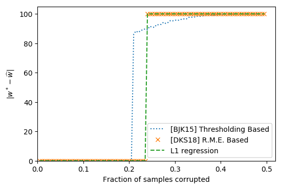
Figure 2: Empirically in the one-dimensional case, the recovery threshold for ℓ1\ell_{1} regression and the robust mean estimation-based algorithm of [DKS18] match at η0\eta_{0}.

We compare the tolerance of ℓ1\ell_{1} regression to algorithms from two recent papers [DKS18] and [BJK15]. We study the fraction of corruptions these algorithms can tolerate in the limit of a large number of samples. Our experiment is the following - we study the one-dimensional case where w∗=100w^{*}=100 and the adversarial noise is selected by setting the largest η\eta fraction of observed yy’s to 00. We run the three algorithms on a dataset of 10001000 samples for η\eta ranging from 00 to 0.50.5 and consider the point when the algorithm stops providing exact recovery. In Figure 2 we plot the the error of the recovered w^\widehat{w} from w∗w^{*} against the fraction of corruptions.

While the fraction of corruptions tolerated by the algorithm from [BJK15] for our example is more than what they prove in general (which is 165\frac{1}{65}), the fraction of corruptions it can tolerate is still less than that of ℓ1\ell_{1} regression on this example. For ℓ1\ell_{1} regression we observe what we have already proven earlier, that this example achieves our upper bound - i.e. it tolerates no more than an η0≈0.239\eta_{0}\approx 0.239 fraction of corruptions.

Curiously, the robust mean estimation based algorithm by [DKS18] on this example tolerates exactly the same fraction of corruptions as ℓ1\ell_{1} regression.

Acknowledgements

The authors would like to thank the anonymous reviewers and Aravind Gollakota for helpful suggestions and comments about the writeup.

References

  • [BJK15] Kush Bhatia, Prateek Jain, and Purushottam Kar. Robust regression via hard thresholding. In Advances in Neural Information Processing Systems, pages 721–729, 2015.
  • [BJKK17] Kush Bhatia, Prateek Jain, Parameswaran Kamalaruban, and Purushottam Kar. Consistent robust regression. In I. Guyon, U. V. Luxburg, S. Bengio, H. Wallach, R. Fergus, S. Vishwanathan, and R. Garnett, editors, Advances in Neural Information Processing Systems 30, pages 2110–2119. Curran Associates, Inc., 2017.
  • [BS80] P. Bloomfield and W. Steiger. Least absolute deviations curve-fitting. SIAM Journal on Scientific and Statistical Computing, 1(2):290–301, 1980.
  • [CRT06] E. J. Candès, J. Romberg, and T. Tao. Stable signal recovery from incomplete and inaccurate measurements. Comm. Pure Appl. Math., 59(8):1208–1223, 2006.
  • [DKK+18] Ilias Diakonikolas, Gautam Kamath, Daniel M. Kane, Jerry Li, Jacob Steinhardt, and Alistair Stewart. Sever: A robust meta-algorithm for stochastic optimization. CoRR, abs/1803.02815, 2018.
  • [DKS18] I. Diakonikolas, W. Kong, and A. Stewart. Efficient Algorithms and Lower Bounds for Robust Linear Regression. ArXiv e-prints, May 2018.
  • [DMT07] Cynthia Dwork, Frank McSherry, and Kunal Talwar. The price of privacy and the limits of lp decoding. In Proceedings of the thirty-ninth annual ACM symposium on Theory of computing, pages 85–94. ACM, 2007.
  • [FM14] Rina Foygel and Lester Mackey. Corrupted sensing: Novel guarantees for separating structured signals. IEEE Transactions on Information Theory, 60(2):1223–1247, 2014.
  • [Hub11] Peter J Huber. Robust statistics. In International Encyclopedia of Statistical Science, pages 1248–1251. Springer, 2011.
  • [KKM18] Adam R. Klivans, Pravesh K. Kothari, and Raghu Meka. Efficient algorithms for outlier-robust regression. In Conference On Learning Theory, COLT 2018, Stockholm, Sweden, 6-9 July 2018., pages 1420–1430, 2018.
  • [LDB09] Jason N Laska, Mark A Davenport, and Richard G Baraniuk. Exact signal recovery from sparsely corrupted measurements through the pursuit of justice. In Signals, Systems and Computers, 2009 Conference Record of the Forty-Third Asilomar Conference on, pages 1556–1560. IEEE, 2009.
  • [Li13] Xiaodong Li. Compressed sensing and matrix completion with constant proportion of corruptions. Constructive Approximation, 37(1):73–99, 2013.
  • [LSLC18] Liu Liu, Yanyao Shen, Tianyang Li, and Constantine Caramanis. High dimensional robust sparse regression. arXiv preprint arXiv:1805.11643, 2018.
  • [NT13] Nam H Nguyen and Trac D Tran. Exact recoverability from dense corrupted observations via l1-minimization. IEEE transactions on information theory, 59(4):2017–2035, 2013.
  • [NTN11] Nasser M Nasrabadi, Trac D Tran, and Nam Nguyen. Robust lasso with missing and grossly corrupted observations. In Advances in Neural Information Processing Systems, pages 1881–1889, 2011.
  • [WLJ07] Hansheng Wang, Guodong Li, and Guohua Jiang. Robust regression shrinkage and consistent variable selection through the lad-lasso. Journal of Business & Economic Statistics, 25(3):347–355, 2007.
  • [WXT10] Meng Wang, Weiyu Xu, and Ao Tang. The limits of error correction with lp decoding. CoRR, abs/1006.0277, 2010.
  • [YY17] Chun Yu and Weixin Yao. Robust linear regression: A review and comparison. Communications in Statistics-Simulation and Computation, 46(8):6261–6282, 2017.

Appendix

Appendix A Facts about N(0,1)

In this section, let Φ\Phi and Φ^\widehat{\Phi} denote the CDF of N⁡(0,1)N(0,1) and the CDF of the uniform distribution over a set of samples drawn from N⁡(0,1)N(0,1) respectively – the set will be clear from context. B⁡(γ)B(\gamma) and G⁡(γ)G(\gamma) refer to the ℓ1\ell_{1} norm of the largest (in absolute value) γ\gamma fraction of the entries and the smallest 1−γ1-\gamma fraction of the entries with respect to the Gaussian distribution, and G^​(γ)\widehat{G}(\gamma) and B^​(γ)\widehat{B}(\gamma) are defined similarly but for the uniform distribution over samples from N⁡(0,1)N(0,1).

Fact A.1.

Let S={z1,…,zm}S=\{z_{1},\dots,z_{m}\} be i.i.d. samples from N⁡(0,1)N(0,1). Then for any τ,γ∈[0,1]\tau,\gamma\in[0,1] the following holds with probability 1−4​e−2​m​τ21-4e^{-2m\tau^{2}}.

Φ−1​(γ−τ)<Φ^−1​(γ)<Φ−1​(γ+τ).\Phi^{-1}(\gamma-\tau)<\widehat{\Phi}^{-1}(\gamma)<\Phi^{-1}(\gamma+\tau).
Proof.

The Dvoretzky-Kiefer-Wolfowitz inequality states

Pr⁡(supx∈ℝ(|Φ^​(x)−Φ⁡(x)|)>ε)≤2​e−2​m​ε2for every ​ε≥12​m​ln⁡2.\Pr\Bigl(\sup_{x\in\mathbb{R}}\bigl(|\widehat{\Phi}(x)-\Phi(x)|\bigr)>\varepsilon\Bigr)\leq 2e^{-2m\varepsilon^{2}}\qquad\text{for every }\varepsilon\geq\sqrt{\tfrac{1}{2m}\ln 2}. (8)

If t=Φ−1​(η)t=\Phi^{-1}(\eta), Equation 8 then tells us that for any ϵ\epsilon independent of mm (i.e. constant ϵ\epsilon),

Pr⁡(|Φ^​(t)−η|>ε)≤2​e−2​m​ε2\Pr\Bigl(|\widehat{\Phi}(t)-\eta|>\varepsilon\Bigr)\leq 2e^{-2m\varepsilon^{2}}

i.e.

Pr⁡(Φ^​(t)≤η+ϵ)≤2​e−2​m​ε2.\Pr\Bigl(\widehat{\Phi}(t)\leq\eta+\epsilon\Bigr)\leq 2e^{-2m\varepsilon^{2}}.

Setting η=γ−τ\eta=\gamma-\tau and ϵ=τ\epsilon=\tau we see

Pr⁡(Φ^​(t)≤γ)≤2​e−2​m​τ2.\Pr\Bigl(\widehat{\Phi}(t)\leq\gamma\Bigr)\leq 2e^{-2m\tau^{2}}.

Monotonicity of Φ^\widehat{\Phi} then proves the first inequality. The second inequality follows similarly. ∎

Fact A.2.

Let S={z1,…,zm}S=\{z_{1},\dots,z_{m}\} be i.i.d. samples from N⁡(0,1)N(0,1) and let η<η0\eta<\eta_{0}. Then with probability 1−O⁡(em​ϵ22)1-O\left(e^{\frac{m\epsilon^{2}}{2}}\right),

G^​(η)>G⁡(η−ϵ)−ϵ\widehat{G}(\eta)>G(\eta-\epsilon)-\epsilon

and

B^​(η)<B⁡(η+ϵ)+ϵ.\widehat{B}(\eta)<B(\eta+\epsilon)+\epsilon.
Proof.

Consider the random variable YY where YY is N⁡(0,1)N(0,1) conditional from being drawn from [−t,t][-t,t] (i.e. YY has the PDF of a truncated Gaussian distribution). If γ<12\gamma<\frac{1}{2}, for t=Φ−1​(1−γ2)t=\Phi^{-1}(1-\frac{\gamma}{2})

E[|Y|]=11−γ∫−tt|x|e−x2/2dx=11−γG(γ).E[|Y|]=\frac{1}{1-\gamma}\int_{-t}^{t}|x|e^{-x^{2}/2}dx=\frac{1}{1-\gamma}G(\gamma).

Observe that one can sample from YY by sampling from ZZ which is distributed as N⁡(0,1)N(0,1) and discarding samples outside [−t,t][-t,t]. Since the PDF is scaled, we have to scale the empirical distribution as well

E^​[|Y|]=1m⁡(1−γ)​∑i=1m|zi|⋅1[−t,t]​(zi)\widehat{E}[|Y|]=\frac{1}{m(1-\gamma)}\sum_{i=1}^{m}|z_{i}|\cdot 1_{[-t,t]}(z_{i})

Let γ\gamma be such that E​|Y|≤12​(1−γ)E|Y|\leq\frac{1}{2(1-\gamma)}, then |Y||Y| has subgaussian tails with some constant parameter. To see this, observe that

E⁡[eλ⁡(|Y|−E⁡[|Y|])]\displaystyle E\left[e^{\lambda(|Y|-E[|Y|])}\right] =21−γ∫0te−x2/2+λx−λE[|Y|]dx\displaystyle=\frac{2}{1-\gamma}\int_{0}^{t}e^{-x^{2}/2+\lambda x-\lambda E[|Y|]}dx
≲eλ22−(2⋅(1−γ))−1​λ\displaystyle\lesssim e^{\frac{\lambda^{2}}{2}-(2\cdot(1-\gamma))^{-1}\lambda}
≲eO⁡(λ2/2−λ)\displaystyle\lesssim e^{O(\lambda^{2}/2-\lambda)}

This implies concentration for the expectation

Pr⁡(|E^​[|Y|]−E⁡[|Y|]|>ϵ)<O⁡(e−m​ϵ22).\Pr\left(\left|\widehat{E}[|Y|]-E[|Y|]\right|>\epsilon\right)<O\left(e^{-\frac{m\epsilon^{2}}{2}}\right).

Multiplying both sides inside the probability by (1−γ)(1-\gamma) and noting that since γ<12\gamma<\frac{1}{2} this is bounded by 12\frac{1}{2} we see

Pr⁡(|1m​∑i=1m|zi|⋅1[−t,t]​(zi)−G⁡(γ)|>ϵ2)<O⁡(e−m​ϵ22)\Pr\left(\left|\frac{1}{m}\sum_{i=1}^{m}|z_{i}|\cdot 1_{[-t,t]}(z_{i})-G(\gamma)\right|>\frac{\epsilon}{2}\right)<O\left(e^{-\frac{m\epsilon^{2}}{2}}\right)

We now set γ=η−ϵ\gamma=\eta-\epsilon. Since η<η0≈0.239\eta<\eta_{0}\approx 0.239 and ϵ>0\epsilon>0, γ<12\gamma<\frac{1}{2}. Fact A.1 now implies that with probability 1−2​e−2​m​ϵ21-2e^{-2m\epsilon^{2}}, at most an 1−η1-\eta fraction of the samples lie in [−t,t][-t,t]. These have to be smaller in absolute value than the remaining samples. Since G^​(η)\widehat{G}(\eta) is defined to be the ℓ1\ell_{1} norm of the 1−η1-\eta fraction of points smallest in absolute value, we see

G^​(η)>1m​∑i=1m|zi|⋅1[−t,t]​(zi).\widehat{G}(\eta)>\frac{1}{m}\sum_{i=1}^{m}|z_{i}|\cdot 1_{[-t,t]}(z_{i}).

This implies

Pr⁡(G^​(η)>G⁡(η−ϵ)−ϵ)<O⁡(e−2​m​ϵ2+e−m​ϵ22).\Pr\left(\widehat{G}(\eta)>G(\eta-\epsilon)-\epsilon\right)<O\left(e^{-2m\epsilon^{2}}+e^{-\frac{m\epsilon^{2}}{2}}\right).

The other direction is done similarly, however in this case YY is the random variable gotten by conditioning samples from N⁡(0,1)N(0,1) to be outside [−t,t][-t,t]. ∎

Appendix B Shelling argument

Lemma 3.3 (Shelling Argument).

Let A∈ℝm×nA\in\mathbb{R}^{m\times n} satisfy

L​‖v‖2≤‖A​v‖1≤U​‖v‖2L\|v\|_{2}\leq\|Av\|_{1}\leq U\|v\|_{2}

for all (1+α2)​k(1+\alpha^{2})k-sparse vectors vv. If S⊂[m]S\subset[m] is fixed and of cardinality kk, then AA satisfies

L1+α​(α−UL)​‖v‖2−2​U​Δα​k≤‖A​v‖1≤U⁡(1+1α)​‖v‖2+U​Δα​k\frac{L}{1+\alpha}\left(\alpha-\frac{U}{L}\right)\|v\|_{2}-\frac{2U\Delta}{\alpha\sqrt{k}}\leq\|Av\|_{1}\leq U\left(1+\frac{1}{\alpha}\right)\|v\|_{2}+\frac{U\Delta}{\alpha\sqrt{k}}

for all

v∈VS={v∈ℝn∣Δ+‖vS‖1≥‖vS¯‖1}.v\in V_{S}=\{v\in\mathbb{R}^{n}\mid\Delta+\|v_{S}\|_{1}\geq\|v_{\overline{S}}\|_{1}\}.
Proof.

The goal is to transfer bounds from the eigenvalues of AA restricted over the sparse vectors, to the eigenvalues of AA restricted over VSV_{S}. To this end we will select an element of VSV_{S} and express it as a sum of sparse vectors. Applications of standard inequalities will then let us transfer bounds.

For any v∈VSv\in V_{S} partition [n][n] into S,T1,…,Tn−kα2​kS,T_{1},\dots,T_{\frac{n-k}{\alpha^{2}k}} where TiT_{i} is the set of indices corresponding to the it​hi^{th} largest α2​k\alpha^{2}k-sized set of elements from vS¯v_{\overline{S}}.

We will now prove the upper and lower bounds on the eigenvalues for vectors restricted to the set VSV_{S}. The triangle inequality implies

‖A​vS∪T1‖1−∑i>1‖A​vTi‖1≤‖A​v‖1≤‖A​vS∪T1‖1+∑i>1‖A​vTi‖1\|Av_{S\cup T_{1}}\|_{1}-\sum_{i>1}\|Av_{T_{i}}\|_{1}\leq\|Av\|_{1}\leq\|Av_{S\cup T_{1}}\|_{1}+\sum_{i>1}\|Av_{T_{i}}\|_{1}

Since vS∪T1v_{S\cup T_{1}} and vTiv_{T_{i}} are all at most (1+α2)​k(1+\alpha^{2})k-sparse,

L​‖vS∪T1‖2−∑i>1‖A​vTi‖1≤‖A​v‖1≤U​‖vS∪T1‖2+∑i>1‖A​vTi‖1L\|v_{S\cup T_{1}}\|_{2}-\sum_{i>1}\|Av_{T_{i}}\|_{1}\leq\|Av\|_{1}\leq U\|v_{S\cup T_{1}}\|_{2}+\sum_{i>1}\|Av_{T_{i}}\|_{1}

We now prove an upper bound on the quantity ∑i>1‖A​vTi‖1\sum_{i>1}\|Av_{T_{i}}\|_{1}. This will give us both the upper and lower bounds we need. To this end, observe that all coordinates of vTi−1v_{T_{i-1}} are greater than or equal to all coordinates of vTiv_{T_{i}}. This implies

‖vTi‖∞≤‖vTi−1‖1α2​k\|v_{T_{i}}\|_{\infty}\leq\frac{\|v_{T_{i-1}}\|_{1}}{\alpha^{2}k}

which, in turn, implies

‖vTi‖2≤1α​k​‖vTi−1‖1.\|v_{T_{i}}\|_{2}\leq\frac{1}{\alpha\sqrt{k}}\|v_{T_{i-1}}\|_{1}.

Using the bounds on the restricted sparse eigenvalues from the statement, we get

∑i>1‖A​vTi‖1\displaystyle\sum_{i>1}\|Av_{T_{i}}\|_{1} ≤U⋅∑i>1‖vTi‖2\displaystyle\leq U\cdot\sum_{i>1}\|v_{T_{i}}\|_{2}
≤Uα​k​‖vS¯‖1\displaystyle\leq\frac{U}{\alpha\sqrt{k}}\|v_{\overline{S}}\|_{1}
≤Uα​k​(‖vS‖1+Δ)\displaystyle\leq\frac{U}{\alpha\sqrt{k}}\left(\|v_{S}\|_{1}+\Delta\right)
≤Uα⋅‖vS‖2+Uα​k⋅Δ\displaystyle\leq\frac{U}{\alpha}\cdot\|v_{S}\|_{2}+\frac{U}{\alpha\sqrt{k}}\cdot\Delta
≤Uα⋅‖vS∪T1‖2+Uα​k⋅Δ\displaystyle\leq\frac{U}{\alpha}\cdot\|v_{S\cup T_{1}}\|_{2}+\frac{U}{\alpha\sqrt{k}}\cdot\Delta

Using the inequality above in addition to the bounds on ‖A​v‖1\|Av\|_{1}, we get after some rearrangement

(L−Uα)​‖vS∪T1‖2−Uα​k⋅Δ≤‖A​v‖1≤U⁡(1+1α)​‖vS∪T1‖2+Uα​k⋅Δ\left(L-\frac{U}{\alpha}\right)\|v_{S\cup T_{1}}\|_{2}-\frac{U}{\alpha\sqrt{k}}\cdot\Delta\leq\|Av\|_{1}\leq U\left(1+\frac{1}{\alpha}\right)\|v_{S\cup T_{1}}\|_{2}+\frac{U}{\alpha\sqrt{k}}\cdot\Delta

The bounds above are in terms of ‖vS∪T1‖2\|v_{S\cup T_{1}}\|_{2}, however we need bounds in terms of ‖v‖2\|v\|_{2}. For the upper bound, it is sufficient to note that ‖vS∪T1‖2<‖v‖2\|v_{S\cup T_{1}}\|_{2}<\|v\|_{2}. For the lower bound, we need the inequalities below.

The definition of TiT_{i} and applications of the Cauchy-Schwartz inequality gives us

‖vS∪T1¯‖2≤∑i≥2‖vTi‖2≤1α​k​∑i≥1‖vTi−1‖1≤‖vS¯‖1α​k≤‖vS‖1+Δα​k≤‖vS‖2α+Δα​k.\|v_{\overline{S\cup T_{1}}}\|_{2}\leq\sum_{i\geq 2}\|v_{T_{i}}\|_{2}\leq\frac{1}{\alpha\sqrt{k}}\sum_{i\geq 1}\|v_{T_{i-1}}\|_{1}\leq\frac{\|v_{\overline{S}}\|_{1}}{\alpha\sqrt{k}}\leq\frac{\|v_{S}\|_{1}+\Delta}{\alpha\sqrt{k}}\leq\frac{\|v_{S}\|_{2}}{\alpha}+\frac{\Delta}{\alpha\sqrt{k}}.

This, in turn, results in an upper bound on ‖v‖2\|v\|_{2} in terms of ‖vS∪T1‖2\|v_{S\cup T_{1}}\|_{2},

‖v‖2\displaystyle\|v\|_{2} ≤‖vS∪T1‖2+‖vS∪T1¯‖2\displaystyle\leq\|v_{S\cup T_{1}}\|_{2}+\|v_{\overline{S\cup T_{1}}}\|_{2}
≤‖vS∪T1‖2+∑i≥2‖vTi‖2\displaystyle\leq\|v_{S\cup T_{1}}\|_{2}+\sum_{i\geq 2}\|v_{T_{i}}\|_{2}
≤‖vS∪T1‖2+‖vS‖2α+Δα​k\displaystyle\leq\|v_{S\cup T_{1}}\|_{2}+\frac{\|v_{S}\|_{2}}{\alpha}+\frac{\Delta}{\alpha\sqrt{k}}
≤(1+1α)​‖vS∪T1‖2+Δα​k\displaystyle\leq\left(1+\frac{1}{\alpha}\right)\|v_{S\cup T_{1}}\|_{2}+\frac{\Delta}{\alpha\sqrt{k}}
⟹‖vS∪T1‖2≥α1+α​(‖v‖2−Δα​k)\displaystyle\implies\|v_{S\cup T_{1}}\|_{2}\geq\frac{\alpha}{1+\alpha}\left(\|v\|_{2}-\frac{\Delta}{\alpha\sqrt{k}}\right)

and so

L1+α​(α−UL)​(‖v‖2−Δα​k)−U​Δα​k≤‖A​v‖1≤U⁡(1+1α)​‖vS∪T1‖2+U​Δα​k\frac{L}{1+\alpha}\left(\alpha-\frac{U}{L}\right)\left(\|v\|_{2}-\frac{\Delta}{\alpha\sqrt{k}}\right)-\frac{U\Delta}{\alpha\sqrt{k}}\leq\|Av\|_{1}\leq U\left(1+\frac{1}{\alpha}\right)\|v_{S\cup T_{1}}\|_{2}+\frac{U\Delta}{\alpha\sqrt{k}}

At this point, we have the upper bound, to complete the proof of the lower bound, observe that standard manipulations give us

L1+α​(α−UL)​(‖v‖2−Δα​k)\displaystyle\frac{L}{1+\alpha}\left(\alpha-\frac{U}{L}\right)\left(\|v\|_{2}-\frac{\Delta}{\alpha\sqrt{k}}\right) =L1+α​(α−UL)​‖v‖2−L1+α​(α−UL)​Δα​k\displaystyle=\frac{L}{1+\alpha}\left(\alpha-\frac{U}{L}\right)\|v\|_{2}-\frac{L}{1+\alpha}\left(\alpha-\frac{U}{L}\right)\frac{\Delta}{\alpha\sqrt{k}}
=L1+α​(α−UL)​‖v‖2−α​L−U1+α​Δα​k\displaystyle=\frac{L}{1+\alpha}\left(\alpha-\frac{U}{L}\right)\|v\|_{2}-\frac{\alpha L-U}{1+\alpha}\frac{\Delta}{\alpha\sqrt{k}}
≥L1+α​(α−UL)​‖v‖2−U​Δα​k\displaystyle\geq\frac{L}{1+\alpha}\left(\alpha-\frac{U}{L}\right)\|v\|_{2}-\frac{U\Delta}{\alpha\sqrt{k}}

This gives us the Lemma,

L1+α​(α−UL)​‖v‖2−2​U​Δα​k≤‖A​v‖1≤U⁡(1+1α)​‖vS∪T1‖2+U​Δα​k.\frac{L}{1+\alpha}\left(\alpha-\frac{U}{L}\right)\|v\|_{2}-\frac{2U\Delta}{\alpha\sqrt{k}}\leq\|Av\|_{1}\leq U\left(1+\frac{1}{\alpha}\right)\|v_{S\cup T_{1}}\|_{2}+\frac{U\Delta}{\alpha\sqrt{k}}.

∎