Decentralized Optimal Merging Control for Connected and Automated Vehicles

Wei Xiao Christos G. Cassandras ^†^†thanks: *This work was supported in part by NSF under grants ECCS-1509084, IIP-1430145 and CNS-1645681, by AFOSR under grant FA9550-12-1-0113, by ARPA-E’s NEXTCAR program under grant DE-AR0000796, and by Bosch and the MathWorks. Affiliation: The authors are with the Division of Systems Engineering and Center for Information and Systems Engineering, Boston University, Brookline, MA, 02446, USA {xiaowei,cgc}@bu.edu

Abstract

This paper addresses the optimal control of Connected and Automated Vehicles (CAVs) arriving from two roads at a merging point where the objective is to jointly minimize the travel time and energy consumption of each CAV. The solution guarantees that a speed-dependent safety constraint is always satisfied, both at the merging point and everywhere within a control zone which precedes it. We first analyze the case of no active constraints and prove that under certain conditions the safety constraint remains inactive, thus significantly simplifying the determination of an explicit decentralized solution. When these conditions do not apply, an explicit solution is still obtained that includes intervals over which the safety constraint is active. Our analysis allows us to study the tradeoff between the two objective function components (travel time and energy within the control zone). Simulation examples are included to compare the performance of the optimal controller to a baseline with human-driven vehicles with results showing improvements in both metrics.

I INTRODUCTION

Traffic management at merging points (usually, highway on-ramps) is one of the most challenging problems within a transportation system in terms of safety, congestion, and energy consumption, in addition to being a source of stress for many drivers [14, 15, 18]. Advancements in next generation transportation system technologies and the emergence of CAVs (also known as self-driving cars or autonomous vehicles) have the potential to drastically improve a transportation network’s performance by better assisting drivers in making decisions, ultimately reducing energy consumption, air pollution, congestion and accidents. One of the very early efforts exploiting the benefit of CAVs was proposed in [5], where an optimal linear feedback regulator is introduced for the merging problem to control a single string of vehicles. An overview of automated intelligent vehicle-highway systems was provided in [16].

There has been significant research in assisted freeway merging offering guidance to drivers so as to avoid congestion and collisions. A Classification and Regression Tree (CART) method was used in [19] to model merging behavior and assist decisions in terms of the time-to-collision between vehicles. The Long Short-Term Memory (LSTM) network was used in [3] to predict possible long-term congestion. In [21], a Radial Basis Function-Artificial Neural Networks (RBF-ANN) is used to forcast the traffic volume in a merging area. However, such assisted merging methods do not take advantage of autonomous driving so as to possibly automate the merging process in a cooperative manner.

A number of centralized or decentralized merging control mechansims have been proposed [9, 2, 7, 8, 15, 12, 10, 13]. In the case of decentralized control, all computation is performed on board each vehicle and shared only with a small number of other vehicles which are affected by it. Optimal control problem formulations are used in some of these approaches, while Model Predictive Control (MPC) techniques are employed in others, primarily to account for additional constraints and to compensate for disturbances by re-evaluating optimal actions. The objectives specified for optimal control problems may target the minimization of acceleration as in [12] or the maximization of passenger comfort (measured as the acceleration derivative or jerk) as in [9, 11]. MPC approaches have been used in [2, 8], as well as in [9] when inequality constraints are added to the originally considered optimal control problem.

In [25], a decentralized optimal control framework is provided for a signal-free intersection. This may be viewed as a process of merging multiple traffic flows so that the highway merging problem is a special case. However, as detailed in the sequel, there are several differences in the formulation and analysis we pursue here in terms of the objective function and the safety constraints used.

In this paper, we develop a decentralized optimal control framework for each CAV approaching a merging point from one of two roads (often, a highway lane and an on-ramp lane). Our objective differs from formulations in [9], [12] or [25]; moreover, it is designed to guarantee that a hard speed-dependent safety constraint is always satisfied. In particular, our objective combines minimizing $(i)$ the travel time of each CAV over a given road segment from a point entering a Control Zone (CZ) to the eventual Merging Point (MP) and $(ii)$ a measure of its energy consumption. This allows us to explore the trade-off between these two metrics as a function of a weight factor. The problem incorporates CAV speed and acceleration constraints, and a hard safety constraint requiring a minimal headway between adjacent vehicles at all times as well as guaranteed collision avoidance at the MP. We derive an analytical solution of the problem and identify several properties of an optimal trajectory. This allows us to obtain simple to check conditions under which the safe distance constraint is guaranteed to not become active (which significantly reduces computation); in cases where it does become active, we include constrained arcs as part of an optimal trajectory . Thus, we can identify when a trajectory exists that provably satisfies all constraints at all times and explicitly determine the optimal merging trajectory of each CAV.

The paper is structured as follows. In Section II, we present the merging process model and formulate the optimal merging control problem including all safety requirements that must be satisfies at all times. In Section III, the optimal solutions in all cases are presented. We show the simulations and discussion in Section IV and V, respectively.

II PROBLEM FORMULATION

The merging problem arises when traffic must be joined from two different roads, usually associated with a main lane and a merging lane as shown in Fig.1. We consider the case where all traffic consists of CAVs randomly arriving at the two lanes joined at the Merging Point (MP) $M$ where a collison may occur. The segment from the origin $O$ or $O^{\prime}$ to the merging point $M$ has a length $L$ for both lanes, and is called the Control Zone (CZ). We assume that CAVs do not overtake each other in the CZ. A coordinator is associated with the MP whose function is to maintain a First-In-First-Out (FIFO) queue of CAVs based on their arrival time at the CZ and enable real-time communication with the CAVs that are in the CZ as well as the last one leaving the CZ. The FIFO assumption imposed so that CAVs cross the MP in their order of arrival is made for simplicity and often to ensure fairness, but can be relaxed through dynamic resequencing schemes, e.g., as described in [22].

Refer to caption — Fig. 1: The merging problem

Let $S(t)$ be the set of FIFO-ordered indices of all CAVs located in the CZ at time $t$ along with the CAV (whose index is 0 as shown in Fig.1) that has just left the CZ. Let $N(t)$ be the cardinality of $S(t)$ . Thus, if a CAV arrives at time $t$ it is assigned the index $N(t)$ . All CAV indices in $S(t)$ decrease by one when a CAV passes over the MP and the vehicle whose index is $-1$ is dropped.

The vehicle dynamics for each CAV $i\in S(t)$ along the lane to which it belongs take the form

\left[\begin{array}[c]{c}\dot{x}_{i}(t)\\ \dot{v}_{i}(t)\end{array}\right]=\left[\begin{array}[c]{c}v_{i}(t)\\ u_{i}(t)\end{array}\right]

(1)

where $x_{i}(t)$ denotes the distance to the origin $O$ ( $O^{\prime}$ ) along the main (merging) lane if the vehicle $i$ is located in the main (merging) lane, $v_{i}(t)$ denotes the velocity, and $u_{i}(t)$ denotes the control input (acceleration). We consider two objectives for each CAV subject to three constraints, as detailed next.

$\mathbf{Objective1}$ (Minimizing travel time): Let $t_{i}^{0}$ and $t_{i}^{m}$ denote the time that CAV $i\in S(t)$ arrives at the origin $O$ or $O^{\prime}$ and the merging point $M$ , respectively. We wish to minimize the travel time $t_{i}^{m}-t_{i}^{0}$ for CAV $i$ .

$\mathbf{Objective2}$ (Minimizing energy consumption): We also wish to minimize energy consumption for each CAV $i\in S(t)$ expressed as

J_{i}(t_{i}^{m},u_{i}(t))=\int_{t_{i}^{0}}^{t_{i}^{m}}C(u_{i}(t))dt,

(2)

where $C(\cdot)$ is a strictly increasing function of its argument.

$\mathbf{Constraint1}$ (Safety constraints): Let $i_{p}$ denote the index of the CAV which physically immediately precedes $i$ in the CZ (if one is present). We require that the distance $z_{i,i_{p}}(t):=x_{i_{p}}(t)-x_{i}(t)$ be constrained by the speed $v_{i}(t)$ of CAV $i\in S(t)$ so that

z_{i,i_{p}}(t)\geq\varphi v_{i}(t)+\delta,\text{ \ }\forall t\in[t_{i}^{0},t_{i}^{m}],

(3)

where $\varphi$ denotes the reaction time (as a rule, $\varphi=1.8$ is used, e.g., [17]). If we define $z_{i,i_{p}}$ to be the distance from the center of CAV $i$ to the center of CAV $i_{p}$ , then $\delta$ is a constant determined by the length of these two CAVs (generally dependent on $i$ and $i_{p}$ but taken to be a constant over all CAVs for simplicity).

$\mathbf{Constraint2}$ (Safe merging): There should be enough safe space at the MP $M$ for a merging CAV to cut in, i.e.,

z_{1,0}(t_{1}^{m})\geq\varphi v_{1}(t_{1}^{m})+\delta.

(4)

$\mathbf{Constraint3}$ (Vehicle limitations): Finally, there are constraints on the speed and acceleration for each $i\in S(t)$ , i.e.,

	$\displaystyle v_{min}\leq v_{i}(t)\leq v_{max},\forall t\in[t_{i}^{0},t_{i}^{m}],$		(5)
	$\displaystyle u_{min}\leq u_{i}(t)\leq u_{max},\forall t\in[t_{i}^{0},t_{i}^{m}],$		(5)

where $v_{max}>0$ and $v_{min}>0$ denote the maximum and minimum speed allowed in the CZ, while $u_{min}<0$ and $u_{max}>0$ denote the minimum and maximum control input, respectively.

Problem Formulation. Our goal is to determine a control law to achieve objectives 1-2 subject to constraints 1-3 for each $i\in S(t)$ governed by the dynamics (1). Combining objectives 1 and 2, we formulate the following optimal control problem for each CAV:

\min_{u_{i}(t)}J_{i}(t_{i}^{m},u_{i}(t)):=\beta(t_{i}^{m}-t_{i}^{0})+\int_{t_{i}^{0}}^{t_{i}^{m}}\frac{1}{2}u_{i}^{2}(t)dt,

(6)

subject to (1), (3), (4), (5), the initial and terminal position conditions $x_{i}(t_{i}^{0})=0$ , $x_{i}(t_{i}^{m})=L$ , and given $t_{i}^{0},v_{i}(t_{i}^{0})$ . The weight factor $\beta\geq 0$ can be adjusted to penalize travel time relative to the energy cost. The two terms in (6) need to be properly normalized. Thus, by defining $t_{i,max}=L/v_{min}$ to be the maximum travel time and using $\alpha\in[0,1]$ , we construct a convex combination as follows:

	$\displaystyle J_{i}(t_{i}^{m},u_{i}(t))=$	$\displaystyle\alpha\frac{(t_{i}^{m}-t_{i}^{0})}{t_{i,max}}+\frac{(1-\alpha)\int_{t_{i}^{0}}^{t_{i}^{m}}\frac{1}{2}u_{i}^{2}(t)dt}{\frac{1}{2}\max(u_{max}^{2},u_{min}^{2})t_{i,max}}$		(7)
	$\displaystyle=$	$\displaystyle\frac{\alpha\max(u_{max}^{2},u_{min}^{2})}{2(1-\alpha)}(t_{i}^{m}\!-\!t_{i}^{0})\!+\!\int_{t_{i}^{0}}^{t_{i}^{m}}\!\frac{1}{2}u_{i}^{2}(t)dt$		(7)

We can then set $\beta=\frac{\alpha\max(u_{max}^{2},u_{min}^{2})}{2(1-\alpha)}$ and use (6) as the problem to be solved.

III DECENTRALIZED FRAMEWORK

Note that (6) can be locally solved by each CAV $i$ provided that there is some information sharing with two other CAVs: CAV $i_{p}$ which physically immediately precedes $i$ and is needed in (3) and CAV $i-1$ so that $i$ can determine whether this CAV is located in the same lane or not. With this information, CAV $i$ can determine which of two possible cases applies: $(i)$ $i_{p}=i-1$ , i.e., $i_{p}$ is the CAV immediately preceding $i$ in the FIFO queue (e.g., CAVs 3 and 5 in Fig.1), and $(ii)$ $i_{p}<i-1$ , which implies that CAV $i-1$ is in a different lane from $i$ (e.g., CAVs 2 and 4 in Fig.1). It is now clear that we can solve problem (6) for any $i\in S(t)$ in a decentralized way in the sense that CAV $i$ needs only its own local information and information from $i-1$ , as well as from $i_{p}$ in case $(ii)$ . Observe that if $i_{p}=i-1$ , then (4) is a redundant constraint; otherwise, we need to separately consider (3) and (4). Therefore, we will analyze each of these two cases in what follows.

III-A Decentralized Optimal Control when $i-1=i_{p}$

Let $\bm{x}_{i}(t):=(x_{i}(t),v_{i}(t))^{T}$ be the state vector and $\bm{\lambda}_{i}(t):=(\lambda_{i}^{x}(t),\lambda_{i}^{v}(t))^{T}$ be the costate vector (for simplicity, in the sequel we omit explicit time dependence when no ambiguity arises). The Hamiltonian with the state constraint, control constraint and safety constraint adjoined is

$\displaystyle H_{i}(\bm{x}_{i},\bm{\lambda}_{i},u_{i})=$	$\displaystyle\frac{1}{2}u_{i}^{2}\!+\!\lambda_{i}^{x}v_{i}+\lambda_{i}^{v}u_{i}$	(8)
	$\displaystyle+\mu_{i}^{a}(u_{i}\!-\!u_{max})+\mu_{i}^{b}(u_{min}-u_{i})$
	$\displaystyle+\mu_{i}^{c}(v_{i}-v_{max})+\mu_{i}^{d}(v_{min}-v_{i})$
	$\displaystyle+\mu_{i}^{e}(x_{i}+\varphi v_{i}+\delta-x_{i_{p}})+\beta$

The Lagrange multipliers $\mu_{i}^{a},\mu_{i}^{b},\mu_{i}^{c},\mu_{i}^{d},\mu_{i}^{e}$ are positive when the constraints are active and become 0 when the constraints are strict. Note that when the safety constraint (3) becomes active, the expression above involves $x_{i_{p}}(t)$ in the last term. When $i=1$ , the optimal trajectory is obtained without this term, since (3) is inactive over all $[t_{1}^{0},t_{1}^{m}]$ . Thus, once the solution for $i=1$ is obtained (based on the analysis that follows), $x_{1}^{\ast}$ is a given function of time and available to $i=2$ . Based on this information, the optimal trajectory of $i=2$ is obtained. Similarly, all subsequent optimal trajectories for $i>2$ can be recursively obtained based on $x_{i_{p}}^{\ast}(t)$ with $i_{p}=i-1$ .

Since $\psi_{i,1}:=x_{i}(t_{i}^{m})-L=0$ is not an explicit function of time, the transversality condition [1] is

\left.H_{i}(\bm{x}_{i}(t),\bm{\lambda}_{i}(t),u_{i}(t))\right|_{t=t_{i}^{m}}=0

(9)

with the costate boundary condition $\bm{\lambda}_{i}(t_{i}^{m})=[(\nu_{i,1}\frac{\partial\psi_{i,1}}{\partial\bm{x}_{i}})^{T}]_{t=t_{i}^{m}}$ , where $\nu_{i,1}$ denotes a Lagrange multiplier.

The Euler-Lagrange equations become

\dot{\lambda}_{i}^{x}=-\frac{\partial H_{i}}{\partial x_{i}}=-\mu_{i}^{e}

(10)

and

\dot{\lambda}_{i}^{v}=-\frac{\partial H_{i}}{\partial v_{i}}=-\lambda_{i}^{x}-\mu_{i}^{c}+\mu_{i}^{d}-\varphi\mu_{i}^{e},

(11)

and the necessary condition for optimality is

\frac{\partial H_{i}}{\partial u_{i}}=u_{i}+\lambda_{i}^{v}+\mu_{i}^{a}-\mu_{i}^{b}=0.

(12)

$\mathbf{Assumption1:}$ The safety constraint (3), control and state constraints (5) are not active at $t_{i}^{0}$ .

Since CAVs arrive randomly, there are two ways to handle violations of Assumption 1: $(i)$ By ensuring that it holds through a Feasibility Enforcement Zone (FEZ) as in [24] which applies the necessary control prior to the CZ so as to enforce (3) and (5) upon arrival at the CZ, $(ii)$ by foregoing optimality and simply controlling a CAV that violates Assumption 1 until all constraints become feasible within the CZ.

Under Assumption 1, we will start by analyzing the case of no active constraints and then study what happens as different constraints become active. In this paper, we limit ourselves to cases where (3) may become active which are much more challenging than (5); the latter can also be handled through an analysis similar to that found in [6].

III-A1 Control, state, safety constraints not active

In this case, $\mu_{i}^{a}=\mu_{i}^{b}=\mu_{i}^{c}=\mu_{i}^{d}=\mu_{i}^{e}=0$ . Applying (12), the optimal control input is given by

u_{i}+\lambda_{i}^{v}=0.

(13)

and the Euler-Lagrange equation (11) yields

\dot{\lambda}_{i}^{v}=-\lambda_{i}^{x}.

(14)

Therefore, (10) implies $\lambda_{i}^{x}(t)=a_{i}$ , hence $\lambda_{i}^{v}(t)=-(a_{i}t+b_{i})$ , where $a_{i}$ and $b_{i}$ are integration constants. Consequently, we obtain the following optimal solution:

u_{i}^{\ast}(t)=a_{i}t+b_{i}

(15)

v_{i}^{\ast}(t)=\frac{1}{2}a_{i}t^{2}+b_{i}t+c_{i}

(16)

x_{i}^{\ast}(t)=\frac{1}{6}a_{i}t^{3}+\frac{1}{2}b_{i}t^{2}+c_{i}t+d_{i}

(17)

where $c_{i}$ and $d_{i}$ are also integration constants. In addition, we have the initial conditions $x_{i}(t_{i}^{0})=0,v_{i}(t_{i}^{0})=v_{i}^{0}$ and the terminal condition $x_{i}(t_{i}^{m})=L$ . The costate boundary conditions and (12) offer us $u_{i}(t_{i}^{m})=-\lambda_{i}^{v}(t_{i}^{m})=0$ and $\bm{\lambda}_{i}(t_{i}^{m})=(a_{i},0)$ , therefore, the transversality condition (9) gives us an additional relationship:

\beta+a_{i}v_{i}(t_{i}^{m})=0.

(18)

Then, for each $i\in S(t)$ , we need to solve the following five nonlinear algebraic equations for $a_{i},b_{i},c_{i},d_{i}$ and $t_{i}^{m}$ :

		$\displaystyle\frac{1}{2}a_{i}\cdot(t_{i}^{0})^{2}+b_{i}t_{i}^{0}+c_{i}=v_{i}^{0},$		(19)
		$\displaystyle\frac{1}{6}a_{i}\cdot(t_{i}^{0})^{3}+\frac{1}{2}b_{i}\cdot(t_{i}^{0})^{2}+c_{i}t_{i}^{0}+d_{i}=0,$
		$\displaystyle\frac{1}{6}a_{i}\cdot(t_{i}^{m})^{3}+\frac{1}{2}b_{i}\cdot(t_{i}^{m})^{2}+c_{i}t_{i}^{m}+d_{i}=L,$
		$\displaystyle a_{i}t_{i}^{m}+b_{i}=0,$
		$\displaystyle\beta+\frac{1}{2}a_{i}^{2}\cdot(t_{i}^{m})^{2}+a_{i}b_{i}t_{i}^{m}+a_{i}c_{i}=0.$

There may be four, six or eight solutions if we solve (19), depending on the values of $t_{i}^{0},\beta,L$ and $v_{i}^{0}$ , but only one of the solutions is valid, i.e., it satisfies $t_{i}^{m}>t_{i}^{0}$ and $t_{i}^{m}$ is a real number. The remaining solutions are either imaginary or negative numbers. The following six lemmas provide a number of useful properties of the optimal solution (15)-(17).

Observe that when $\beta=0$ , it follows that $a_{i}=0$ from (19). Then, we can easily get the obvious solution

t_{i}^{m}-t_{i}^{0}=\frac{L}{v_{i}^{0}}.

(20)

Lemma 1: The optimal terminal time $t_{i}^{m}$ can be expressed as a polynomial equation in the known parameters $t_{i}^{0}$ , $\beta,L$ and $v_{i}^{0}$ .

$\emph{Proof:}$ If $\beta=0$ , the result is true from (20). If $\beta>0$ , then combining the first and second equations of (19), we get

\frac{1}{3}b_{i}(t_{i}^{0})^{2}+(\frac{2}{3}v_{i}^{0}+\frac{4}{3}c_{i})t_{i}^{0}+2d_{i}=0.

(21)

Combining the third and fourth equations of (19), we get

\frac{1}{3}b_{i}(t_{i}^{m})^{2}+c_{i}t_{i}^{m}+d_{i}=L.

(22)

Combining the last two equations, we get

\frac{1}{3}b_{i}((t_{i}^{m})^{2}-(t_{i}^{0})^{2})+(\frac{2}{3}v_{i}^{0}+\frac{4}{3}c_{i})(t_{i}^{m}-t_{i}^{0})+\frac{b_{i}c_{i}}{3a_{i}}+\frac{2b_{i}v_{i}^{0}}{3a_{i}}=L+d_{i}.

(23)

Subtracting the first equation from the last equation of (19),

\frac{1}{2}a_{i}((t_{i}^{m})^{2}-(t_{i}^{0})^{2})+b_{i}(t_{i}^{m}-t_{i}^{0})=-\frac{\beta}{a_{i}}-v_{i}^{0}.

(24)

Then, combining the last two equations, we get

t_{i}^{m}-t_{i}^{0}=\frac{\frac{a_{i}}{2}(L+d_{i})-\frac{b_{i}c_{i}}{6}+\frac{b_{i}\beta}{3a_{i}}}{\frac{a_{i}v_{i}^{0}}{3}+\frac{2a_{i}c_{i}}{3}-\frac{b_{i}^{2}}{3}}.

(25)

Combining (22) and the last two equations of (19), we get

-\frac{2b_{i}^{3}}{3a_{i}^{2}}+\frac{5b_{i}c_{i}}{3a_{i}}+\frac{2b_{i}\beta}{3a_{i}^{2}}=d_{i}-L

(26)

Taking the square of the fourth equation of (19) and combining with the last equation of (19) yields

b_{i}^{2}=2\beta+2a_{i}c_{i}

(27)

Combining the last two equations, we get

\frac{a_{i}d_{i}}{2}=\frac{a_{i}L}{2}-\frac{b_{i}\beta}{3a_{i}}+\frac{b_{i}c_{i}}{6}

(28)

Combining (28) and (27) with the numerator and denominator of (25), respectively, we get

t_{i}^{m}-t_{i}^{0}=\frac{3a_{i}L}{a_{i}v_{i}^{0}-2\beta}

(29)

Combining (24) and (29), we get

(t_{i}^{m})^{2}-(t_{i}^{0})^{2}=-\frac{2\beta}{a_{i}^{2}}-\frac{2v_{i}^{0}}{a_{i}}-\frac{6b_{i}L}{a_{i}v_{i}^{0}-2\beta}

(30)

Subtracting the second equation from the third equation of (19), we get

\frac{1}{6}a_{i}((t_{i}^{m})^{3}-(t_{i}^{0})^{3})+\frac{1}{2}b_{i}((t_{i}^{m})^{2}-(t_{i}^{0})^{2})+c_{i}(t_{i}^{m}-t_{i}^{0})=L

(31)

Combining (27), (29), (30) and (31) gives

\frac{a_{i}}{6}((t_{i}^{m})^{3}-(t_{i}^{0})^{3})-\frac{b_{i}\beta}{a_{i}^{2}}-\frac{b_{i}v_{i}^{0}}{a_{i}}-\frac{3b_{i}^{2}L+6\beta L}{2(a_{i}v_{i}^{0}-2\beta)}=L

(32)

Rewriting (29) as

a_{i}=\frac{2\beta(t_{i}^{m}-t_{i}^{0})}{(t_{i}^{m}-t_{i}^{0})v_{i}^{0}-3L},

(33)

we notice that $a_{i}$ only depends on $t_{i}^{0},t_{i}^{m},v_{i}^{0},L,\beta$ . Rewriting (30) as

b_{i}=-\left[\frac{(t_{i}^{m})^{2}-(t_{i}^{0})^{2}}{6L}+\frac{\beta+a_{i}v_{i}^{0}}{3a_{i}^{2}L}\right](a_{i}v_{i}^{0}-2\beta),

(34)

we notice $b_{i}$ only depends on $t_{i}^{0},t_{i}^{m},v_{i}^{0},L,\beta,a_{i}$ , because $a_{i}$ only depends on $t_{i}^{0},t_{i}^{m},v_{i}^{0},L,\beta$ . Therefore, $b_{i}$ only depends on $t_{i}^{0},t_{i}^{m},v_{i}^{0},L,\beta$ . In (32), $t_{i}^{m}$ only depends on $t_{i}^{0},v_{i}^{0},L,\beta,a_{i},b_{i}$ . So when solving (32) for $t_{i}^{m}$ with (33) and (34), the solutions only depend on $t_{i}^{0},v_{i}^{0},L,\beta$ . $\;\;\;\qquad\blacksquare$

Lemma 2: The solution for $a_{i}$ in (19) is independent of $t_{i}^{0}$ . Moreover, $a_{i}\leq 0$ .

$\emph{Proof:}$ If $\beta=0$ , then $a_{i}=0$ follows from the last equation of (19). Otherwise, combining (27) and the first equation of (19), we get

a_{i}^{2}(t_{i}^{0})^{2}+2a_{i}b_{i}t_{i}^{0}+b_{i}^{2}-2\beta=2a_{i}v_{i}^{0}.

(35)

Subtracting (35) from the square of the fourth equation of (19), we get

a_{i}^{2}((t_{i}^{m})^{2}-(t_{i}^{0})^{2})+2a_{i}b_{i}(t_{i}^{m}-t_{i}^{0})+2\beta=-2a_{i}v_{i}^{0}.

(36)

Combining the fourth equation of (19), (29) and (36), we get

-a_{i}^{2}(\frac{3a_{i}L}{a_{i}v_{i}^{0}-\beta})^{2}+2\beta=-2a_{i}v_{i}^{0}.

(37)

where $L,\beta,v_{i}^{0}$ are known parameters, and $t_{i}^{0}$ does not appear in (37). Therefore, $a_{i}$ is independent of $t_{i}^{0}$ .

In (18), i.e., $\beta+a_{i}v_{i}(t_{i}^{m})=0$ , since $\beta>0$ and $v_{i}(t_{i}^{m})>0$ , then $a_{i}<0$ . $\qquad\qquad\qquad\qquad\qquad\qquad\qquad\qquad\quad\;\;\blacksquare$

Lemma 3: Given $\beta$ , $L$ and under optimal control (15), if $v_{i}^{0}=v_{j}^{0}$ , then $t_{i}^{m}-t_{j}^{m}=t_{i}^{0}-t_{j}^{0}$ .

$\emph{Proof:}$ If $\beta=0$ , the result is true from (20). Otherwise, by Lemma 2, $a_{i}=a_{j}$ in (29), and $L,\beta$ are known. Since $v_{i}^{0}=v_{j}^{0}$ , it follows that $t_{i}^{m}-t_{j}^{m}=t_{i}^{0}-t_{j}^{0}$ . $\qquad\qquad\qquad\quad\;\;\;\blacksquare$

Lemma 4: Under optimal control (15), $v_{i}(t_{i}^{m})=-\frac{\beta}{a_{i}}$ for all $i\in S(t)$ , and $v_{i}(t)$ is strictly increasing for all $t\in[t_{i}^{0},t_{i}^{m}]$ taking its maximum value at $t=t_{i}^{m}$ when $\beta>0$ . Moreover, $\lim\limits_{\beta\rightarrow 0}\frac{\beta}{-a_{i}}=v_{i}^{0}$ and $\lim\limits_{\beta\rightarrow 0}\frac{3a_{i}L}{a_{i}v_{i}^{0}-2\beta}=\lim\limits_{\beta\rightarrow 0}\frac{3L}{v_{i}^{0}+2v_{i}(t_{i}^{m})}=\frac{L}{v_{i}^{0}}$ .

$\emph{Proof:}$ We know $u_{i}(t_{i}^{m})=0$ from (15) and the fourth equation of (19). By Lemma 2, if $\beta>0$ , we have $a_{i}<0$ , therefore, (15) implies $u_{i}(t)>0$ for all $t\in[t_{i}^{0},t_{i}^{m})$ , hence $v_{i}(t)$ is strictly increasing for all $t\in[t_{i}^{0},t_{i}^{m}]$ and takes its maximum value at $t=t_{i}^{m}$ . From (18), we know $v_{i}(t_{i}^{m})=-\frac{\beta}{a_{i}}$ . Since $v_{i}(t)$ is strictly increasing for all $t\in[t_{i}^{0},t_{i}^{m}]$ when $\beta\neq 0$ , we have $v_{i}(t_{i}^{m})>v_{i}(t_{i}^{0})$ . From (33), we can get $\lim\limits_{\beta\rightarrow 0}a_{i}=0$ , and further $\lim\limits_{\beta\rightarrow 0}b_{i}=0$ from the fourth equation of (19). Finally, we can get $\lim\limits_{\beta\rightarrow 0}u_{i}(t)=0$ from (15), thus, $\lim\limits_{\beta\rightarrow 0}\frac{\beta}{-a_{i}}=\lim\limits_{\beta\rightarrow 0}v_{i}(t_{i}^{m})=v_{i}^{0}$ and $\lim\limits_{\beta\rightarrow 0}\frac{3a_{i}L}{a_{i}v_{i}^{0}-2\beta}=\frac{L}{v_{i}^{0}}$ . $\qquad\qquad\qquad\qquad\qquad\qquad\qquad\qquad\qquad\qquad\quad\;\;\;\;\blacksquare$

Lemma 5: Under optimal control (15), the travel time for $i\in S(t)$ satisfies $t_{i}^{m}-t_{i}^{0}\leq\frac{L}{v_{i}^{0}}$ .

$\emph{Proof:}$ If $\beta=0$ , then $t_{i}^{m}-t_{i}^{0}=\frac{L}{v_{i}^{0}}$ from (20). Otherwise, by Lemma 4, we know $\lim\limits_{\beta\rightarrow 0}t_{i}^{m}-t_{i}^{0}=\frac{L}{v_{i}^{0}}$ . Because $\beta$ is the penalty of $t_{i}^{m}-t_{i}^{0}$ in (6), if $\beta$ increases, then $t_{i}^{m}-t_{i}^{0}$ must decrease or stay the same. Therefore, $t_{i}^{m}-t_{i}^{0}\leq\frac{L}{v_{i}^{0}}$ . $\qquad\blacksquare$

Lemma 6: For two vehicles $i,j\in S(t)$ under optimal control (15), if $v_{i}^{0}<v_{j}^{0}$ and $\beta>0$ , then $v_{i}(t_{i}^{m})<v_{j}(t_{j}^{m})$ , $t_{i}^{m}-t_{i}^{0}>t_{j}^{m}-t_{j}^{0}$ and $a_{i}<a_{j}<0$ .

$\emph{Proof:}$ We rewrite (37) as

9a_{i}^{4}L^{2}=2a_{i}^{3}(v_{i}^{0})^{3}-6a_{i}^{2}(v_{i}^{0})^{2}\beta+8\beta^{3}.

(38)

By Lemma 4, we know $v_{i}(t_{i}^{m})=-\frac{\beta}{a_{i}}$ , and the equality above becomes

\frac{9}{2}\beta L^{2}=4(v_{i}(t_{i}^{m}))^{4}-3(v_{i}(t_{i}^{m}))^{2}(v_{i}^{0})^{2}-v_{i}(t_{i}^{m})(v_{i}^{0})^{3}

(39)

which can be rewritten as

	$\displaystyle\frac{9}{2}\beta L^{2}=3(v_{i}(t_{i}^{m}))^{2}((v_{i}(t_{i}^{m}))^{2}-(v_{i}^{0})^{2})$		(40)
	$\displaystyle+v_{i}(t_{i}^{m})((v_{i}(t_{i}^{m}))^{3}-(v_{i}^{0})^{3}).$		(40)

By Lemma 4, $v_{i}(t_{i}^{m})>v_{i}^{0}$ , Therefore, if $v_{i}^{0}$ decreases, $v_{i}(t_{i}^{m})$ must decrease in order to satisfy (40) whose left hand side is fixed. Formally, by taking the derivative with respect to $v_{i}^{0}$ in (40), we get

\frac{\partial v_{i}(t_{i}^{m})}{\partial v_{i}^{0}}=\frac{6(v_{i}(t_{i}^{m}))^{2}v_{i}^{0}+3v_{i}(t_{i}^{m})(v_{i}^{0})^{2}}{16(v_{i}(t_{i}^{m}))^{3}-6v_{i}(t_{i}^{m})(v_{i}^{0})^{2}-(v_{i}^{0})^{3}}

(41)

By Lemma 4 and (5), $v_{i}(t_{i}^{m})>v_{i}^{0}>0$ , therefore, both the denominator and numerator of (41) are positive, hence $\frac{\partial v_{i}(t_{i}^{m})}{\partial v_{i}^{0}}>0$ . Since $v_{i}(t_{i}^{m})$ is a strictly increasing function with respect to $v_{i}^{0}$ , if $v_{i}^{0}<v_{j}^{0}$ , it follows that $v_{i}(t_{i}^{m})<v_{j}(t_{j}^{m})$ . Further by (18) and (29), $t_{i}^{m}-t_{i}^{0}=\frac{3L}{v_{i}^{0}+2v_{i}(t_{i}^{m})}$ , therefore, $t_{i}^{m}-t_{i}^{0}>t_{j}^{m}-t_{j}^{0}$ . By Lemma 2, $a_{i}<0$ and $a_{j}<0$ . Since $v_{i}(t_{i}^{m})=\frac{\beta}{-a_{i}}$ , it follows that $a_{i}<a_{j}<0$ . $\;\blacksquare$

Using Lemmas 1-6, we can establish Theorem 1 identifying conditions such that the safety constraint (3) is never violated for all $t\in[t_{i}^{0},t_{i}^{m}]$ in an optimal trajectory. The following assumption requires that if two CAVs arrive too close to each other, then the first one maintains its optimal terminal speed past the MP until the second one crosses it as well. This is to ensure that the first vehicle does not suddenly decelerate and cause the safety constraint to be violated during the last segment of the first vehicle’s optimal trajectory.

Assumption 2: For a given constant $\zeta>\varphi$ , any CAV $i-1\in S(t)$ such that $t_{i}^{0}-t_{i-1}^{0}<\zeta$ maintains a constant speed $v_{i-1}(t)=v_{i-1}^{\ast}(t_{i-1}^{m})$ for all $t\in[t_{i-1}^{m},t_{i}^{m}]$ .

Theorem 1: Under Assumptions 1-2, if CAVs $i$ and $i_{p}$ satisfy $v_{i}^{0}\leq v_{i_{p}}^{0}$ and $t_{i}^{0}-t_{ip}^{0}\geq\varphi+\frac{\delta}{v_{i}^{0}}$ , then, under optimal control (15), $z_{i,i_{p}}(t)\geq\varphi v_{i}(t)+\delta$ for all $t\in[t_{i}^{0},t_{i}^{m}]$ . Moreover, if $\beta>0$ , then $z_{i,i_{p}}(t)>\varphi v_{i}(t)+\delta$ for all $t\in[t_{i}^{0},t_{i}^{m}]$ .

$\emph{Proof:}$ If $\beta=0$ , it follows from (18) that $a_{i}=a_{i_{p}}=0$ , and by the costate boundary conditions, we have $b_{i}=0$ . Therefore, it follows from (15) that $u_{i}(t)=u_{i_{p}}(t)=0$ , which impies $v_{i}(t)=v_{i}^{0}$ and $v_{i_{p}}(t)=v_{i_{p}}^{0}$ for all $t\in[t_{i}^{0},t_{i}^{m}]$ . Because $t_{i}^{0}-t_{ip}^{0}\geq\varphi+\frac{\delta}{v_{i}^{0}}$ and $v_{i}^{0}\leq v_{i_{p}}^{0}$ , it follows that $z_{i,i_{p}}(t)\geq\varphi v_{i}(t)+\delta$ for all $t\in[t_{i}^{0},t_{i}^{m}]$ .

If $\beta>0$ , let us first consider the case $v_{i}^{0}=v_{i_{p}}^{0}$ . Since $t_{i}^{0}-t_{ip}^{0}\geq\varphi+\frac{\delta}{v_{i}^{0}}$ , by Lemma 4, $v_{i_{p}}(t)$ is strictly increasing, therefore, $z_{i,i_{p}}(t_{i}^{0})=\int_{t_{ip}^{0}}^{t_{i}^{0}}v_{i_{p}}(t)dt>\int_{t_{ip}^{0}}^{t_{i}^{0}}v_{i_{p}}^{0}dt\geq\varphi v_{i}^{0}+\delta$ , which implies the safety constraint (3) is strict at $t_{i}^{0}$ . Since we have $v_{i}^{0}=v_{i_{p}}^{0}$ , by Lemma 3, $t_{i}^{m}-t_{ip}^{m}=t_{i}^{0}-t_{ip}^{0}\geq\varphi+\frac{\delta}{v_{i}^{0}}$ . By Assumption 2, $z_{i,i_{p}}(t_{i}^{m})=(t_{i}^{m}-t_{i_{p}}^{m})v_{i_{p}}(t_{i_{p}}^{m})$ . By Lemma 2, $a_{i}=a_{i_{p}}$ , and by Lemma 4, $v_{i}(t_{i}^{m})=v_{i_{p}}(t_{i_{p}}^{m})$ , therefore, $z_{i,i_{p}}(t_{i}^{m})=(t_{i}^{m}-t_{i_{p}}^{m})v_{i}(t_{i}^{m})\geq\varphi v_{i}(t_{i}^{m})+\frac{\delta}{v_{i}^{0}}v_{i}(t_{i}^{m})>\varphi v_{i}(t_{i}^{m})+\delta$ . The safety constraint (3) is also strict at $t_{i}^{m}$ . Because $a_{i}=a_{i_{p}}$ and recalling that $u_{i}(t_{i}^{m})=-\lambda_{i}^{v}(t_{i}^{m})=0$ , hence $u_{i}(t_{i}^{m})=u_{i_{p}}(t_{i_{p}}^{m})=0$ , CAVs $i$ and $i_{p}$ have the same control law in the CZ, which implies they will take the same time to arrive at the same point with the same speed in the CZ. Now, considering any time instant $\tau_{i}\in(t_{i}^{0},t_{i}^{m})$ and $\tau_{i_{p}}\in(t_{i_{p}}^{0},t_{i_{p}}^{m})$ such that $\tau_{i}-t_{i}^{0}=\tau_{i_{p}}-t_{i_{p}}^{0}$ , we have $\tau_{i}-\tau_{i_{p}}=t_{i}^{0}-t_{i_{p}}^{0}\geq\varphi+\frac{\delta}{v_{i}^{0}}$ . Because $v_{i_{p}}(t)$ is strictly increasing, it follows that $z_{i,i_{p}}(\tau_{i})=\int_{\tau_{i_{p}}}^{\tau_{i}}v_{i_{p}}(t)dt>(\tau_{i}-\tau_{i_{p}})v_{i_{p}}(\tau_{i_{p}})$ . Because $v_{i}(\tau_{i})=v_{i_{p}}(\tau_{i_{p}})$ , then, $z_{i,i_{p}}(\tau_{i})>(\tau_{i}-\tau_{i_{p}})v_{i}(\tau_{i})\geq\varphi v_{i}(\tau_{i})+\frac{\delta}{v_{i}^{0}}v_{i}(\tau_{i})>\varphi v_{i}(\tau_{i})+\delta$ and the safety constraint (3) is always strict, i.e., $z_{i,i_{p}}(t)>\varphi v_{i}(t)+\delta$ for all $t\in[t_{i}^{0},t_{i}^{m}]$ .

Next, we consider the case $\beta>0$ and $v_{i}^{0}<v_{i_{p}}^{0}$ . Suppose there are two vehicles $i$ and $j$ such that $t_{i}^{0}=t_{j}^{0}$ and $v_{i}^{0}<v_{j}^{0}$ , and both use the optimal controller (15). By Lemma 6, $a_{i}<a_{j}<0$ , $v_{i}(t_{i}^{m})<v_{j}(t_{j}^{m})$ and $t_{i}^{m}>t_{j}^{m}$ . Because $u_{i}(t_{i}^{m})=0$ and $u_{i}(t)=a_{i}t+b_{i}$ , we get $u_{i}(t)=a_{i}(t-t_{i}^{m})$ . Similarly, $u_{j}(t)=a_{j}(t-t_{j}^{m})$ . If $t=t_{i}^{m}$ , because $t_{i}^{m}>t_{j}^{m}$ , then $u_{i}(t_{i}^{m})=0>a_{j}(t_{i}^{m}-t_{j}^{m})=u_{j}(t_{i}^{m})$ . If $t<t_{i}^{m}$ , because $t_{i}^{m}>t_{j}^{m}$ , then $t-t_{i}^{m}<t-t_{j}^{m}$ and $t-t_{i}^{m}<0$ . Because $a_{i}<a_{j}<0$ , then $a_{i}(t-t_{i}^{m})>a_{j}(t-t_{j}^{m})$ , thus $u_{i}(t)>u_{j}(t)$ for all $t\in[t_{i}^{0},t_{i}^{m}]$ . Because $v_{i}^{0}<v_{j}^{0}$ and $v_{i}(t_{i}^{m})<v_{j}(t_{j}^{m})$ , then the speed curves of vehicles $i$ and $j$ will never intersect, i.e., $v_{i}(t)<v_{j}(t)$ for all $t\in[t_{i}^{0},t_{i}^{m}]$ , otherwise, there will be some time such that $u_{j}(t)\geq u_{i}(t)$ , which contradicts $u_{j}(t)<u_{i}(t)$ for all $t\in[t_{i}^{0},t_{i}^{m}]$ . Now, considering the vehicle $j$ to be the case such that $v_{j}(t_{j}^{m})=v_{i_{p}}(t_{i_{p}}^{m})$ and $t_{j}^{0}-t_{i_{p}}^{0}\geq\varphi+\frac{\delta}{v_{j}^{0}}$ , then the safety constraint (3) of $j$ will be satisfied for all $t\in[t_{j}^{0},t_{j}^{m}]\cup(t_{j}^{m},t_{i}^{m}]$ following from the last paragraph and Assumption 2, i.e., $z_{j,i_{p}}(t)>\varphi v_{j}(t)+\delta$ . Because $v_{i}(t)<v_{j}(t)$ for all $t\in[t_{i}^{0},t_{i}^{m}]$ , then $z_{i,i_{p}}(t)>z_{j,i_{p}}(t)$ , hence $z_{i,i_{p}}(t)>z_{j,i_{p}}(t)>\varphi v_{j}(t)+\delta>\varphi v_{i}(t)+\delta$ . Therefore, $z_{i,i_{p}}(t)>\varphi v_{i}(t)+\delta$ for all $t\in[t_{i}^{0},t_{i}^{m}]$ . $\qquad\qquad\qquad\qquad\qquad\qquad\qquad\qquad\qquad\qquad\;\;\blacksquare$

Remark 1: The significance of Theorem 1 is in ensuring that the safety constraint (3) is strict for all $t\in[t_{i}^{0},t_{i}^{m}]$ when $\beta>0$ , $v_{i}^{0}\leq v_{i_{p}}^{0}$ , $t_{i}^{0}-t_{ip}^{0}\geq\varphi+\frac{\delta}{v_{i}^{0}}$ and the optimal control (15) is applied to $i$ and $i_{p}$ . Therefore, in this case we do not need to consider the safety constraint throughout the optimal trajectory, a fact which significantly reduces computation. In contrast, when these conditions are not satisfied, we need to consider the possibility of constrained arcs on the optimal trajectory where $z_{i,i_{p}}(t)=\varphi v_{i}(t)+\delta$ . This case is discussed in the next subsection.

Numerical Example: We have conducted simulations to solve (19) in MATLAB to evaluate the travel time and $v_{i}(t_{i}^{m})$ when we change $\beta$ (or $\alpha$ ) and $v_{i}^{0}$ . As $\beta$ varies with $v_{i}^{0}=20m/s,t_{i}^{0}=0s,L=400$ , the result is shown in Fig.2. The result of changing the initial speed $v_{i}^{0}$ is shown in Fig.3, with $\beta=2.667$ ( $\alpha=0.26$ when $u_{max}=-u_{min}=0.4\times 9.81$ ), $t_{i}^{0}=0s,L=400$ .

III-A2 Safety Constraint Active

When Theorem 1 does not apply, we must check whether the safety constraint (3) between vehicles $i$ and $i_{p}$ is ever violated for some $t\in[t_{i}^{0},t_{i}^{m}]$ when they are under the optimal control (15). If (3) is violated, then we proceed as follows.

Suppose the safety constraint (3) becomes active on an optimal trajectory at some time $t_{1}\in(t_{i}^{0},t_{i}^{m}]$ (where $t_{1}$ will be optimally determined), i.e., defining

g_{i}(t):=x_{i}(t)+\varphi v_{i}(t)+\delta-x_{i_{p}}(t).

(42)

we have $g_{i}(t)<0$ for $t\in[t_{i}^{0},t_{1})$ and $g_{i}(t_{1})=0$ . Taking a time derivative, we get

\frac{dg_{i}(t)}{dt}=v_{i}(t)+\varphi u_{i}(t)-v_{i_{p}}(t)=0

(43)

and it follows that over an optimal trajectory arc such that $g_{i}(t)=0$ , the optimal control is

u_{i}^{\ast}(t)=\frac{v_{i_{p}}(t)-v_{i}^{\ast}(t)}{\varphi},\text{ \ }t\geq t_{1}

(44)

therefore,

\dot{v}_{i}^{\ast}(t)=\frac{v_{i_{p}}(t)-v_{i}^{\ast}(t)}{\varphi},\text{ \ }t\geq t_{1}.

(45)

Clearly, if the original unconstrained optimal trajectory obtained through (15), (16), (17) and (18) violates (3) at any $t\in[t_{i}^{0},t_{i}^{m}]$ with $t_{i}^{m}$ evaluated through (18), then a new optimal trajectory needs to be derived over the entire interval $[t_{i}^{0},t_{i}^{m}]$ . This is done by decomposing this trajectory into an initial segment $[t_{i}^{0},t_{1})$ (where $t_{1}$ is to be determined as part of the optimization process) followed by an arc where (3) is active.

Let us first assume that this arc applies over $[t_{1},t_{i}^{m}]$ and we proceed as follows. We first solve the optimal control problem over $[t_{i}^{0},t_{1})$ with initial conditions $x_{i}(t_{i}^{0}),v_{i}(t_{i}^{0})$ and the terminal constraint $g_{i}(t_{1})=0$ together with the constraints (3), (5). In this solution, we treat $t_{1}$ as a parameter and obtain a solution dependent on $t_{1}$ . We will then derive the optimal value of $t_{1}$ .

Let us assume (5) are inactive, as we did in obtaining (15). Moreover, (3) is inactive since we have assumed it becomes active at some $t_{1}>t_{i}^{0}$ . We can, therefore, derive $x_{i}^{\ast}(t),v_{i}^{\ast}(t),u_{i}^{\ast}(t)$ (all functions of $t_{1}$ ) which are similar to (15)-(17) for all $t\in[t_{i}^{0},t_{1})$ .

Let $\bm{x}_{i}:=(x_{i},v_{i})^{T}$ , $\bm{\lambda}_{i}:=(\lambda_{i}^{x},\lambda_{i}^{v})^{T}$ . Following the notation and analysis of state inequalities in [1], we write the state inequality constraint as $S_{i}(\bm{x}(t)):=x_{i}(t)+\varphi v_{i}(t)+\delta-x_{i_{p}}(t)\leq 0$ and its first derivative as $S_{i}^{(1)}(\bm{x}(t),u_{i}(t))=v_{i}(t)+\varphi u_{i}(t)-v_{i_{p}}(t)$ . The new Hamiltonian is

H_{i}(\bm{x}_{i},\bm{\lambda}_{i},u_{i})=\frac{1}{2}u_{i}^{2}+\lambda_{i}^{x}v_{i}+\lambda_{i}^{v}u_{i}+\beta+\mu S_{i}^{(1)},

(46)

for $t\in[t_{1},t_{i}^{m}]$ . The tangency constraint is $N_{i}(\bm{x}_{i}(t_{1})):=x_{i}(t_{1})+\varphi v_{i}(t_{1})+\delta-x_{i_{p}}(t_{1})=0$ .

Following [1], at the entry point $t_{1}$ , we have

\left.\bm{\lambda}_{i}^{T}(t_{1}^{-})=\bm{\lambda}_{i}^{T}(t_{1}^{+})+\pi\frac{\partial N_{i}}{\partial\bm{x}_{i}}\right|_{t=t_{1}},

(47)

\left.H_{i}(t_{1}^{-})=H_{i}(t_{1}^{+})-\pi\frac{\partial N_{i}}{\partial t}\right|_{t=t_{1}}.

(48)

where $\pi$ is a constant Lagrange multiplier.

By (47), we have

\lambda_{i}^{x}(t_{1}^{-})=\lambda_{i}^{x}(t_{1}^{+})+\pi,

(49)

\lambda_{i}^{v}(t_{1}^{-})=\lambda_{i}^{v}(t_{1}^{+})+\pi\varphi,

(50)

and by (48), we have

	$\displaystyle\frac{1}{2}u_{i}^{2}(t_{1}^{-})+\lambda_{i}^{x}(t_{1}^{-})v_{i}(t_{1})+\lambda_{i}^{v}(t_{1}^{-})u_{i}(t_{1}^{-})=\frac{1}{2}u_{i}^{2}(t_{1}^{+})$
	$\displaystyle+\lambda_{i}^{x}(t_{1}^{+})v_{i}(t_{1})+\lambda_{i}^{v}(t_{1}^{+})u_{i}(t_{1}^{+})+\pi v_{i_{p}}(t_{1}).$

Combining (49), the optimality condition $u_{i}(t_{1}^{-})=-\lambda_{i}^{v}(t_{1}^{-})$ and the last equation, we have

	$\displaystyle-\frac{1}{2}u_{i}^{2}(t_{1}^{-})+\pi v_{i}(t_{1})=$
	$\displaystyle\frac{1}{2}u_{i}^{2}(t_{1}^{+})+\lambda_{i}^{v}(t_{1}^{+})u_{i}(t_{1}^{+})+\pi v_{i_{p}}(t_{1}),$

On the constrained arc, we have from (44): $u_{i}(t_{1}^{+})=\frac{v_{i_{p}}(t_{1})-v_{i}(t_{1})}{\varphi}.$ Therefore, the last equation can be rewritten as

-\frac{1}{2}u_{i}^{2}(t_{1}^{-})=\frac{1}{2}u_{i}^{2}(t_{1}^{+})+\lambda_{i}^{v}(t_{1}^{+})u_{i}(t_{1}^{+})+\varphi\pi u_{i}(t_{1}^{+})

Combining (50) and the last equation, we have

-\frac{1}{2}u_{i}^{2}(t_{1}^{-})=\frac{1}{2}u_{i}^{2}(t_{1}^{+})+\lambda_{i}^{v}(t_{1}^{-})u_{i}(t_{1}^{+})

Further by optimality condition $u_{i}(t_{1}^{-})=-\lambda_{i}^{v}(t_{1}^{-})$ , the last equation can be rewitten as

-\frac{1}{2}u_{i}^{2}(t_{1}^{-})=\frac{1}{2}u_{i}^{2}(t_{1}^{+})-u_{i}(t_{1}^{-})u_{i}(t_{1}^{+})

By simplifying the last equation, we get

u_{i}(t_{1}^{-})=u_{i}(t_{1}^{+})

(51)

Recall that the optimal solution for $t\in[t_{i}^{0},t_{1})$ is given by

		$\displaystyle u_{i}(t)=a_{i}t+b_{i}$		(52)
		$\displaystyle v_{i}(t)=\frac{1}{2}a_{i}t^{2}+b_{i}t+c_{i}$
		$\displaystyle x_{i}(t)=\frac{1}{6}a_{i}t^{3}+\frac{1}{2}b_{i}t^{2}+c_{i}t+d_{i}$

On the constrained arc, we can then solve (45) for the optimal solution $v_{i}^{\ast}(t)$ with initial condition $v_{i}(t_{1})$ known from (52), and hence obtain $x_{i}^{\ast}(t)$ with initial condition $x_{i}(t_{1})$ from (52). Suppose $i_{p}$ is under unconstrained optimal control (15), $v_{i_{p}}^{*}(t)$ is known to CAV $i$ . Moreover, by Assumption 2, we know that $v_{i_{p}}^{*}(t)$ is a constant over $[t_{i_{p}}^{m},t_{i}^{m}]$ . Therefore, we need to divide the solution over two intervals, i.e., the explicit solution for CAV $i$ is:

		$\displaystyle x_{i}^{}(t)=\left\{\!\begin{array}[]{lcl}\begin{aligned} &-c_{v_{1}}\varphi e^{-\frac{1}{\varphi}t}+x_{i_{p}}^{}(t)-d_{i_{p}}-\\ &\varphi(v_{i_{p}}^{}(t)-c_{i_{p}})+a_{i_{p}}\varphi^{2}t+c_{x_{1}}\end{aligned}&t\in[t_{1},t_{i_{p}}^{m}]\\ -c_{v_{2}}\varphi e^{-\frac{1}{\varphi}t}+v_{i_{p}}^{}(t_{i_{p}}^{m})t+c_{x_{2}}&t\in(t_{i_{p}}^{m},t_{i}^{m}]\end{array}\right.$		(53)
		$\displaystyle v_{i}^{}(t)=\left\{\!\begin{array}[]{lcl}c_{v_{1}}e^{-\frac{1}{\varphi}t}\!+\!v_{i_{p}}^{}(t)\!-\!\varphi u_{i_{p}}^{}(t)\!+\!a_{i_{p}}\varphi^{2}&t\in[t_{1},t_{i_{p}}^{m}]\\ c_{v_{2}}e^{-\frac{1}{\varphi}t}+v_{i_{p}}^{}(t_{i_{p}}^{m})&t\in(t_{i_{p}}^{m},t_{i}^{m}]\end{array}\right.$
		$\displaystyle u_{i}^{}(t)=\left\{\begin{array}[]{lcl}-\frac{c_{v_{1}}}{\varphi}e^{-\frac{1}{\varphi}t}+u_{i_{p}}^{}(t)-\varphi a_{i_{p}}&t\in[t_{1},t_{i_{p}}^{m}]\\ -\frac{c_{v_{2}}}{\varphi}e^{-\frac{1}{\varphi}t}&t\in(t_{i_{p}}^{m},t_{i}^{m}]\end{array}\right.$

where $c_{x_{1}}=x_{i}^{*}(t_{1})+c_{v_{1}}\varphi e^{-\frac{1}{\varphi}t_{1}}-x_{i_{p}}^{*}(t_{1})+d_{i_{p}}+\varphi(v_{i_{p}}^{*}(t_{1})-c_{i_{p}})-a_{i_{p}}\varphi^{2}t_{1}$ , $c_{x_{2}}=x_{i}^{*}(t_{i_{p}}^{m})+c_{v_{2}}\varphi e^{-\frac{1}{\varphi}t_{i_{p}}^{m}}-v_{i_{p}}^{*}(t_{i_{p}}^{m})t_{i_{p}}^{m}$ , $c_{v_{1}}=e^{\frac{1}{\varphi}t_{1}}(v_{i}^{*}(t_{1})-v_{i_{p}}^{*}(t_{1})+\varphi u_{i_{p}}^{*}(t_{1})-a_{i_{p}}\varphi^{2})$ , $c_{v_{2}}=e^{\frac{1}{\varphi}t_{i_{p}}^{m}}(v_{i}^{*}(t_{i_{p}}^{m})-v_{i_{p}}^{*}(t_{i_{p}}^{m}))$ . If $i_{p}$ is also under constrained optimal control, the optimal solution for $i$ is recursively determined by (45) starting from the first vehicle that is under unconstrained optimal control.

The value of the entry point $t_{1}$ can be directly obtained by combining (51), initial conditions, terminal conditions and the tangency constraint $N_{i}(\bm{x}_{i}(t_{1}))$ , i.e., we have the following algebraic equations

		$\displaystyle a_{i}t_{1}+b_{i}=\frac{v_{i_{p}}(t_{1})-v_{i}(t_{1})}{\varphi},$		(54)
		$\displaystyle\frac{1}{2}a_{i}\cdot(t_{i}^{0})^{2}+b_{i}t_{i}^{0}+c_{i}=v_{i}^{0},$
		$\displaystyle\frac{1}{6}a_{i}\cdot(t_{i}^{0})^{3}+\frac{1}{2}b_{i}\cdot(t_{i}^{0})^{2}+c_{i}t_{i}^{0}+d_{i}=0,$
		$\displaystyle x_{i}(t_{1})+\varphi v_{i}(t_{1})+\delta=x_{i_{p}}(t_{1}),$
		$\displaystyle\varphi v_{i}(t_{i}^{m})+\delta=v_{i_{p}}(t_{i_{p}}^{m})(t_{i}^{m}-t_{i_{p}}^{m}),$
		$\displaystyle x_{i}(t_{i}^{m})=L.$

to solve for $a_{i},b_{i},c_{i},d_{i},t_{1},t_{i}^{m}$ .

In what follows, we first assume that $i_{p}$ is under unconstrained optimal control. Solving (54) generally provides multiple solutions for $t_{1}$ , some of which may not be feasible. Since we have assumed $i_{p}$ is under unconstrained optimal control, we know that $\frac{dg_{i}(t)}{dt}$ is a quadratic funtion, and there are total six cases as shown in Fig. 4. By (51), we have $\frac{dg_{i}(t)}{dt}|_{t=t_{1}}=0$ , thus, $\frac{dg_{i}(t)}{dt}$ must intersect with time axis at $t_{1}$ . We can, therefore, exclude these two cases where $\frac{dg_{i}(t)}{dt}$ does not intersect the time axis as shown in Fig. 4. By Assumption 1, the safety constraint is strict at $t_{i}^{0}$ , therefore, we have $g_{i}(t_{i}^{0})<0$ , $g_{i}(t)$ cannot decrease for all $t\in[t_{i}^{0},t_{1})$ such that $g_{i}(t_{1})=0$ , so we can exclude another case that is also shown in Fig. 4. Now, we have three cases for $\frac{dg_{i}(t)}{dt}$ , if $t_{1}$ locates at $t_{1}^{\textcircled{3}}$ shown in Fig.4, then $t_{1}$ is not the first time such that the safety constraint (3) becomes active, which is infeasible. The remaining possible locations for $t_{1}$ shown in Fig. 4 are feasible.

However, as we can see in (53), the last two equations in (54) are exponential functions of time as we have already assumed the constrained arc (53) has no exit point. Consequently, they are hard to solve directly. This motivates an alternative approach in which we first solve the first four equations in (54) for $a_{i},b_{i},c_{i},d_{i}$ in terms of $t_{1}$ :

		$\displaystyle a_{i}t_{1}+b_{i}=\frac{v_{i_{p}}(t_{1})-v_{i}(t_{1})}{\varphi},$		(55)
		$\displaystyle\frac{1}{2}a_{i}\cdot(t_{i}^{0})^{2}+b_{i}t_{i}^{0}+c_{i}=v_{i}^{0},$
		$\displaystyle\frac{1}{6}a_{i}\cdot(t_{i}^{0})^{3}+\frac{1}{2}b_{i}\cdot(t_{i}^{0})^{2}+c_{i}t_{i}^{0}+d_{i}=0,$
		$\displaystyle x_{i}(t_{1})+\varphi v_{i}(t_{1})+\delta=x_{i_{p}}(t_{1}).$

Similarly as in (54), the optimal control (52) solved by (55) for $t\in[t_{i}^{0},t_{1})$ cannot guarantee that $t_{1}$ is the first time such that the safety constraint (3) becomes active (if that happens, then $t_{1}$ is infeasible). Therefore, we need to exclude such infeasible $t_{1}$ as explained next.

Under Assumption 1, there may exist some cases such that $v_{i}(t_{1}^{-})<v_{i_{p}}(t_{1}^{-})$ when the safety constraint (3) becomes active between CAV $i$ and $i_{p}$ . By Assumption 1, it follows that $g_{i}(t_{i}^{0})<0$ . We also have $g_{i}(t_{1})=0$ . However, the sign of the derivative $\left.\frac{dg_{i}(t)}{dt}\right|_{t=t_{1}^{-}}$ is unknown. If $\left.\frac{dg_{i}(t)}{dt}\right|_{t=t_{1}^{-}}\geq 0$ i.e., $v_{i}(t_{1}^{-})+\varphi u_{i}(t_{1}^{-})\geq v_{i_{p}}(t_{1}^{-})$ , it is possible that $v_{i}(t_{1}^{-})<v_{i_{p}}(t_{1}^{-})$ when $u_{i}(t_{1})>0$ . Similarly, if $\left.\frac{dg_{i}(t)}{dt}\right|_{t=t_{1}^{-}}<0$ , there is also a possibility that $v_{i}(t_{1}^{-})<v_{i_{p}}(t_{1}^{-})$ . This property is helpful to understand the process of finding the infeasible set for $t_{1}$ .

Definition 1: We define a set $I_{i}$ as:

\displaystyle I_{i}:=

\displaystyle\{t_{1}\in(t_{i}^{0},t_{i}^{m}]|u_{i}(t_{1})+\varphi a_{i}>u_{i_{p}}^{*}(t_{1})\},

(56)

where $u_{i}(t_{1})$ is from (52).

Lemma 7: Under Assumption 1, if $I_{i}$ is non-empty, then any $t_{1}\in I_{i}$ is not the first time such that the safety constraint (3) becomes active.

$\emph{Proof:}$ Since the safety constraint (3) becomes active at $t_{1}\in I$ , it follows that $g_{i}(t_{1})=0$ . By the first equation of (54), we have $\left.\frac{dg_{i}(t)}{dt}\right|_{t=t_{1}^{-}}=0$ . If $u_{i}(t_{1})+\varphi a_{i}>u_{i_{p}}(t_{1})$ , i.e., $\left.\frac{d^{2}g_{i}(t)}{dt^{2}}\right|_{t=t_{1}^{-}}>0$ , then the function $g_{i}(t)\rightarrow 0$ as $t\rightarrow t_{1}$ from the positive side. By the continuity of $g_{i}(t)$ , we know that the safety constraint is violated for some $t<t_{1}$ . By Assumption 1, the safety constraint (3) is initially strict, thus, there exist time instant $t_{a}<t_{1}$ such that $g_{i}(t_{a})=0$ . Therefore, any $t_{1}\in\{t_{1}\in(t_{i}^{0},t_{i}^{m}]|u_{i}(t_{1})+\varphi a_{i}>u_{i_{p}}^{*}(t_{1})\}$ is not the first time such that the safety constraint (3) becomes active. $\;\;\;\;\blacksquare$

We know that $t_{1}\in I_{i}$ is infeasible since these $t_{1}$ will make the safety constraint (3) become violated for a time interval. Therefore, we need to exclude $I_{i}$ for the safety constraint active case.

Theorem 2: Under Assumption 1, $g_{i}(t_{1})=0$ and $\left.\frac{dg_{i}(t)}{dt}\right|_{t=t_{1}^{-}}\geq 0$ are the necessary conditions for $t_{1}$ to be the first time such that the safety constraint (3) becomes active. Moreover, if CAV $i_{p}$ is under unconstrained optimal control (15), $g_{i}(t_{1})=0$ , $\left.\frac{dg_{i}(t)}{dt}\right|_{t=t_{1}^{-}}=0$ and $\left.\frac{d^{2}g_{i}(t)}{dt^{2}}\right|_{t=t_{1}^{-}}\leq 0$ are sufficient conditions.

$\emph{Proof:}$ If $t_{1}$ is the first time such that the safety constraint (3) becomes active, then it follows that $g_{i}(t_{1})=0$ . By Assumption 1, we have $g_{i}(t_{i}^{0})<0$ . If $\left.\frac{dg_{i}(t)}{dt}\right|_{t=t_{1}^{-}}<0$ , then we have $g_{i}(t_{1}^{-})>0$ . By the continuity of $g_{i}(t)$ , it follows that we have another time instant $t_{a}<t_{1}$ such that the safety constraint (3) becomes active, which contradicts the fact that $t_{1}$ is the first time. Therefore, we have $\left.\frac{dg_{i}(t)}{dt}\right|_{t=t_{1}^{-}}\geq 0$ , thus, $g_{i}(t_{1})=0$ and $\left.\frac{dg_{i}(t)}{dt}\right|_{t=t_{1}^{-}}\geq 0$ are the necessary conditions.

By (52), it follows that $v_{i}(t)$ is a second order polynomial funtion of time. Since CAV $i_{p}$ is under unconstrained optimal control (15), it follows from (16) that $v_{i_{p}}^{*}(t)$ is also a second order polynomial function of time for $t\in[t_{i_{p}}^{0},t_{i_{p}}^{m}]$ and $v_{i_{p}}^{*}(t)=v_{i_{p}}^{*}(t_{i_{p}}^{m})$ for $t\in[t_{i_{p}}^{m},t_{i}^{m}]$ following from Assumption 1. Therefore, $\frac{dg_{i}(t)}{dt}$ is a second order polynomial funtion of time for $t\in[t_{i}^{0},t_{1})$ . By Lemma 7, $\left.\frac{d^{2}g_{i}(t)}{dt^{2}}\right|_{t=t_{1}^{-}}\leq 0$ indicates that $t_{1}\notin I_{i}$ , and further by $\left.\frac{dg_{i}(t)}{dt}\right|_{t=t_{1}^{-}}=0$ , we have $\frac{dg_{i}(t)}{dt}>0,\forall t\in[t_{i}^{0},t_{1})$ or $\frac{dg_{i}(t)}{dt}$ is negative for $t\in[t_{i}^{0},t_{a})$ and becomes positive for $t\in(t_{a},t_{1})$ (where $t_{a}\in(t_{i}^{0},t_{1})$ ). By Assumption 1, the safety constraint (3) is strict at $t_{i}^{0}$ . Thus, $g_{i}(t)<0,\forall t\in[t_{i}^{0},t_{1})$ and $t_{1}$ is the only time such that the safety constraint (3) becomes active for $t\in[t_{i}^{0},t_{1}]$ . Therefore, if CAV $i_{p}$ is under unconstrained optimal control (15), $g_{i}(t_{1})=0$ , $\left.\frac{dg_{i}(t)}{dt}\right|_{t=t_{1}^{-}}=0$ and $\left.\frac{d^{2}g_{i}(t)}{dt^{2}}\right|_{t=t_{1}^{-}}<0$ are sufficient conditions for $t_{1}$ to be the first time that the safety constraint (3) becomes active. $\;\;\;\blacksquare$

Remark 2: Theorem 2 applies only to the case where $i_{p}$ is not under constrained optimal control, i.e., the safety constraint (3) never became active. If this does not hold, then the form of $\frac{dg_{i}(t)}{dt}$ is no longer quadratic, in which case we need to identify the set $I_{i}$ by determining all $t_{1}\in(t_{i}^{0},t_{i}^{m}]$ such that there exists $t\in[t_{i}^{0},t_{1})$ that $g_{i}(t)>0$ . Clearly, the computation effort for fully determining $I_{i}$ is more intensive in such cases.

Theorem 2 provides simple to check conditions to find all feasible $t_{1}$ that are the first time such that the safety constraint (3) becomes active. Otherwise, we need to do more computation to decide whether $t_{1}$ is feasible or not, as suggested in Remark 2.

Recall that we have assumed that there is no exit point from this constraint arc prior to $t_{i}^{m}$ . Using the optimal solutions (52) for $[t_{i}^{0},t_{1})$ and (44) for $[t_{1},t_{i}^{m}]$ in (6), we obtain the optimal value of the objective function $J_{i}^{\ast}(t_{1})$ parameterized by $t_{1}$ :

	$\displaystyle J_{i}^{*}(t_{1})\!=\!\beta(t_{i}^{m}\!-\!t_{i}^{0})\!+\!\frac{a_{i}^{2}}{6}(t_{1}^{3}\!-\!(t_{i}^{0})^{3})\!+\!\frac{1}{2}a_{i}b_{i}(t_{1}^{2}\!-\!(t_{i}^{0})^{2})$		(57)
	$\displaystyle+\frac{1}{2}b_{i}^{2}(t_{1}-t_{i}^{0})+\int_{t_{1}}^{t_{i_{p}}^{m}}\frac{1}{2}(u_{i}^{}(t))^{2}dt+\int_{t_{i_{p}}^{m}}^{t_{i}^{m}}\frac{1}{2}(u_{i}^{}(t))^{2}dt$		(57)

where $u_{i}^{\ast}(t)$ is the optimal control from (44) and depends on $t_{1}$ as do the constants $a_{i},b_{i}$ above. $u_{i}^{\ast}(t)$ is also a function of $t_{1}$ for $t\in[t_{1},t_{i_{p}}^{m}]$ as its explicit solution shown in (53). The optimal solution for $t_{1}$ is obtained by finding $t_{1}$ that minimizes $J_{i}^{\ast}(t_{1})$ . Note that the value of $t_{i}^{m}$ is obtained by setting $x_{i}^{\ast}(t_{i}^{m})=L$ . If we apply the optimal controller (44) till $t_{i}^{m}$ , then $t_{i}^{m}$ is also dependent on $t_{1}$ as the explicit solution of $x_{i}^{\ast}(t_{i}^{m})$ shown in (53).

If $t_{1}^{*}=t_{i}^{m}$ , then the interior point $t_{1}$ degenerates to a terminal point. We then need to take the safety constraint as a terminal boundary constraint and solve a new optimal control problem that will be discussed in Sec.III-B.

Let us now explore the case where there exists an exit point from the constraint arc (44) prior to $t_{i}^{m}$ . First, observe that $t_{1}$ is the first instant when CAV $i$ catches up with $i_{p}$ so as to activate (3), therefore $v_{i}(t_{1})\geq v_{i_{p}}(t_{1})$ . It is easy to see that if $u_{i}^{\ast}(t)$ in (44) remains negative, then (44) remains the optimal solution. However, if $v_{i_{p}}(t_{2})>v_{i}(t_{2})$ at some $t_{2}\in[t_{1},t_{i}^{m}]$ , this means that it is possible (44) is no longer optimal because the safety constraint (3) may become inactive again. In this case, we need to solve another optimal control problem similar to that of the no-active-constraint case (15)-(17) but with initial condition $x_{i}(t_{2})$ obtained from the solution of (45), with the same terminal conditions as in (6), subject to (1), (3) and (5), and with $t_{i}^{m}$ once again a free terminal time. For the new arc starting at $t_{2}$ , we can solve for $a_{i},b_{i},c_{i},d_{i},t_{i}^{m}$ and $t_{2}$ similar to (19) using

		$\displaystyle\frac{1}{2}a_{i}t_{2}^{2}+b_{i}t_{2}+c_{i}=v_{i}^{*}(t_{2}),$		(58)
		$\displaystyle\frac{1}{6}a_{i}t_{2}^{3}+\frac{1}{2}b_{i}t_{2}^{2}+c_{i}t_{2}+d_{i}=x_{i}^{*}(t_{2}),$
		$\displaystyle\frac{1}{6}a_{i}\cdot(t_{i}^{m})^{3}+\frac{1}{2}b_{i}\cdot(t_{i}^{m})^{2}+c_{i}t_{i}^{m}+d_{i}=L,$
		$\displaystyle a_{i}t_{i}^{m}+b_{i}=0,$
		$\displaystyle\beta+\frac{1}{2}a_{i}^{2}\cdot(t_{i}^{m})^{2}+a_{i}b_{i}t_{i}^{m}+a_{i}c_{i}=0,$
		$\displaystyle a_{i}t_{2}+b_{i}=u_{i}^{*}(t_{2})$

where $x_{i}^{\ast}(t_{2})$ , $v_{i}^{\ast}(t_{2})$ , $u_{i}^{\ast}(t_{2})$ are the optimal solutions from (44)-(45) and the last equation ensures the continuity of $u_{i}(t)$ , otherwise, the safety constraint (3) is immediately violated. If a feasible solution for $t_{2}$ exists in solving (58), then we evaluate the objective (6) again as in (57) in order to determine the optimal values of $t_{1}$ and $t_{2}$ ; otherwise, the trajectory determined above over $[t_{1},t_{i}^{m}]$ is optimal.

If a feasible solution for $t_{2}$ is determined, it is possible that the safety constraint (3) becomes active again at some $t_{3}\in[t_{2},t_{i}^{m}]$ . Thus, we use the same method to deal with the construction of a complete optimal trajectory recursively.

In a nutshell, we can summarize the method of finding the optimal $t_{1}$ (or $t_{2}$ if it exists) and $x_{i}^{*}(t),v_{i}^{*}(t),u_{i}^{*}(t)$ by Algorithm 1, which includes all cases, including the case when $i_{p}$ is under constrained optimal control, or even recursively constrained optimal control.

Algorithm 1 Safety constrained optimal trajectory,

i_{p}=i-1

Input: $t_{i}^{0},v_{i}^{0},x_{i_{p}}^{*}(t),v_{i_{p}}^{*}(t),u_{i_{p}}^{*}(t)$
Output: $t_{1}^{*},x_{i}^{*}(t),v_{i}^{*}(t),u_{i}^{*}(t)$ , $t_{2}^{*}$ (if it exists)

1: solve (55)

2: if CAV

i_{p}

is under unconstrained optimal control (15) then

I_{i}:=\{t_{1}\in(t_{i}^{0},t_{i}^{m}]|u_{i}(t_{1})+\varphi a_{i}>u_{i_{p}}^{*}(t_{1})\}

4: else

I_{i}=\{t_{1}\in(t_{i}^{0},t_{i}^{m}]|\exists t\in[t_{i}^{0},t_{1}),g_{i}(t)>0\}

6: get feasible set

F_{i}:=(t_{i}^{0},t_{i}^{m})\setminus I_{i}

for

t_{1}

7: solve (53) or its recursive form if

i_{p}

is under constrained optimal control

8: solve (58)

9: if (58) has no feasible solutions (

t_{2}

does not exist) then

10: solve

t_{i}^{m}

in terms of

t_{1}

x_{i}^{*}(t_{i}^{m})=L

11: get

J_{i}^{*}(t_{1})

by (57)

12: solve for

t_{1}^{*}

over

F_{i}

13: result =

t_{1}^{*},x_{i}^{*}(t),v_{i}^{*}(t),u_{i}^{*}(t)

14: else

15: get

J_{i}^{*}(t_{1})

by a similar form as (57)

16: solve for

t_{1}^{*}

over

F_{i}

(and

t_{2}^{*}

)

17: result =

t_{1}^{*},x_{i}^{*}(t),v_{i}^{*}(t),u_{i}^{*}(t),t_{2}^{*}

18: if

t_{1}^{*}=t_{i}^{m}

then

19: take the safety constraint (3) as a terminal boundary constraint as in Sec.III-B

20: if the safety constraint (3) is satisfied

\forall t\in[t_{i}^{0},t_{i}^{m}]

then

21: result =

t_{1}^{*}(=t_{i}^{m}),x_{i}^{*}(t),v_{i}^{*}(t),u_{i}^{*}(t)

22: return result

The next theorem ensures that if an optimal trajectory includes an arc over which the safety constraint (3) is initially satisfied, then the optimal control (44) never violates the constraint (5).

Theorem 3: If $u_{min}\leq\frac{v_{i_{p}}(t_{1})-v_{i}(t_{1})}{\varphi}\leq u_{max}$ , then under optimal control (44) for $t\in[t_{1},t_{i}^{m}]$

, $u_{min}\leq u_{i}^{\ast}(t)\leq u_{max}$ .

$\emph{Proof:}$ Taking a time derivative in (44) we get

\dot{u}_{i}(t)=\frac{u_{i_{p}}(t)-u_{i}(t)}{\varphi},t\geq t_{1}.

(59)

with $u_{i}(t_{1})\geq u_{min}$ . There are three cases to consider.

Case 1: $u_{i}(t_{1})=u_{min}$ , so that $\dot{u}_{i}(t)=\frac{u_{i_{p}}(t)-u_{min}}{\varphi}$ . Because $u_{min}\leq u_{i_{p}}(t)\leq u_{max}$ on an optimal trajectory for vehicle $i_{p}$ , we get $\dot{u}_{i}(t)\geq 0$ , which means $u_{i}(t)$ is non-decreasing.

Case 2: $u_{i}(t_{1})=u_{max}$ , so that $\dot{u}_{i}(t)=\frac{u_{i_{p}}(t)-u_{max}}{\varphi}$ . Because $u_{min}\leq u_{i_{p}}(t)\leq u_{max}$ on an optimal trajectory for vehicle $i_{p}$ , we get $\dot{u}_{i}(t)\leq 0$ , which means $u_{i}(t)$ is non-increasing.

Case 3: $u_{min}<u_{i}(t_{1})<u_{max}$ . In this case, we have $\dot{u}_{i}(t)\geq\frac{u_{min}-u_{i}(t_{1})}{\varphi}$ and $\dot{u}_{i}(t)$ may be negative, therefore, $u_{i}(t)$ is allowed to decrease when $u_{i}(t)>u_{min}$ . But when $u_{i}(t)$ approaches $u_{min}$ , the lower bound of $\dot{u}_{i}(t)$ will approach zero and $u_{i}(t)$ is once again non-decreasing, therefore, $u_{i}(t)\geq u_{min}$ for all $t\in[t_{1},t_{i}^{m}]$ . On the other hand, we also have $\dot{u}_{i}(t)\leq\frac{u_{max}-u_{i}(t_{1})}{\varphi}$ and $\dot{u}_{i}(t)$ may be positive, therefore, $u_{i}(t)$ is allowed to increase when $u_{i}(t)<u_{max}$ . But when $u_{i}(t)$ approaches $u_{max}$ , the upper bound of $\dot{u}_{i}(t)$ will approach zero, then $u_{i}(t)$ is once again non-increasing, therefore, $u_{i}(t)\leq u_{max}$ , $\forall t\in[t_{1},t_{i}^{m}]$ . $\quad\blacksquare$

Numerical Example: The initial parameters for $i$ and $i_{p}$ are with $i_{p}=i-1$ , $t_{i_{p}}^{0}=0s$ , $v_{i_{p}}^{0}=20m/s,$ $t_{i}^{0}=2.7s,$ $v_{i}^{0}=27m/s$ , $\beta=2.667$ ( $\alpha=0.2573$ ), $\varphi=1.8s$ , $\delta=0m$ , $L=400m$ . If we apply (15), we know that the safety constraint (3) will be violated. Therefore, we need to solve for the constrained optimal control. We use (52) for $t\in[t_{i}^{0},t_{1})$ , (53) for $t\in[t_{1},t_{2})$ and the optimal control solved by (58) for $t\in[t_{2},t_{i}^{m}]$ . Firstly, we check whether there is infeasible interval $I_{i}$ for $t_{1}$ , as shown in Fig.5.

It follows from Fig.5 that the infeasible interval $I_{i}=(10.5,t_{i}^{m}]$ does exist in this case, then $F_{i}=[t_{i}^{0},t_{i}^{m}]\setminus I_{i}$ . Because $v_{i}(t_{1})<v_{i_{p}}(t_{1})$ , $\forall t_{1}\in F_{i}$ , then $t_{2}$ exists following from Theorem 4. It follows from (58) that $t_{2}$ depends on $t_{1}$ and $t_{i}^{m}$ is free. The optimal objective function with respect to $t_{1}$ is shown in Fig.6, and we get $t_{1}^{*}=9.25s$ .

We continue to study the state and safety constraint profiles at $t_{1}^{*}=9.25s$ and $t_{2}^{*}=15.76s$ , as shown in Fig.7-10.

III-B Decentralized Optimal Control when $i-1>i_{p}$

In this case, CAV $i_{p}$ which physically precedes $i\in S(t)$ is different from $i-1$ which, therefore, is in a different lane than $i$ . This implies that we need to consider the safe merging constraint (4) at $t=t_{i}^{m}$ . We define a new state vector $\bm{x}_{i}(t):=(x_{i}(t),v_{i}(t))^{T}$ . We also define a new terminal constraint $\psi_{i,2}(\bm{x}_{i}(t_{i}^{m}),t_{i}^{m}):=x_{i}(t_{i}^{m})+\varphi v_{i}(t_{i}^{m})+\delta-x_{i-1}(t_{i}^{m})=0$ , where we have replaced the inequality in (4) by an equality in order to seek the most efficient safe merging possible and $x_{i-1}(t_{i}^{m})$ is known (an explicit function of time).

Let $\bm{\psi}_{i}:=(\psi_{i,1},\psi_{i,2})^{T}$ , $\bm{\nu}_{i}:=(\nu_{i,1},\nu_{i,2})^{T}$ and define the costate $\bm{\lambda}_{i}:=(\lambda_{i}^{x},\lambda_{i}^{v})^{T}$ . The Hamiltonian with the constraints adjoined is

$\displaystyle H_{i}(\bm{x}_{i},\bm{\lambda}_{i},u_{i})=$	$\displaystyle\frac{1}{2}u_{i}^{2}+\lambda_{i}^{x}v_{i}+\lambda_{i}^{v}u_{i}$	(60)
	$\displaystyle+\!\mu_{i}^{a}(u_{i}\!-\!u_{max})\!+\!\mu_{i}^{b}(u_{min}\!-\!u_{i})$
	$\displaystyle+\mu_{i}^{c}(v_{i}-v_{max})+\mu_{i}^{d}(v_{min}-v_{i})$
	$\displaystyle+\mu_{i}^{e}(x_{i}+\varphi v_{i}-x_{i_{p}})+\beta$

III-B1 Control, state, safety constraints not active

In this case, $\mu_{i}^{a}=\mu_{i}^{b}=\mu_{i}^{c}=\mu_{i}^{d}=\mu_{i}^{e}=0$ . Applying the optimality condition, we get the same results as (13)-(17).

Since $\psi_{i,2}$ is an explicit function of time ( $x_{i-1}(t_{i}^{m})$ is an explicit function of time), the transversality condition is

\left.\bm{\nu}_{i}^{T}\frac{\partial\bm{\psi}_{i}}{\partial t}+H_{i}(\bm{x}_{i}(t),\bm{\lambda}_{i}(t),u_{i}(t))\right|_{t=t_{i}^{m}}=0

(61)

with the costate boundary condition $\bm{\lambda}_{i}(t_{i}^{m})=[(\bm{\nu}_{i}^{T}\frac{\partial\bm{\psi}_{i}}{\partial\bm{x}_{i}})^{T}]_{t=t_{i}^{m}}$ .

We get $\frac{\partial\bm{\psi}_{i}}{\partial\bm{x}_{i}}$ and $\frac{\partial\bm{\psi}_{i}}{\partial t}$ by:

\frac{\partial\bm{\psi}_{i}}{\partial\bm{x}_{i}}=\left[\begin{matrix}1&0\\ 1&\varphi\end{matrix}\right],\frac{\partial\bm{\psi}_{i}}{\partial t}=\left[\begin{matrix}0\\ -v_{i-1}(t_{i}^{m})\end{matrix}\right]

(62)

By the costate boundary condition, we have

\bm{\lambda}_{i}(t_{i}^{m})=\left[\begin{matrix}\nu_{i,1}(t_{i}^{m})+\nu_{i,2}(t_{i}^{m})\\ \varphi\nu_{i,2}(t_{i}^{m})\end{matrix}\right]

(63)

By (13)-(17), it follows that $\lambda_{i}^{x}(t_{i}^{m})=a_{i},\lambda_{i}^{v}(t_{i}^{m})=-u_{i}(t_{i}^{m})$ , and by (63), we have $\nu_{i,2}(t_{i}^{m})=\frac{1}{\varphi}\lambda_{i}^{v}(t_{i}^{m})$ .

Then, the transversality condition (61) is explicitly rewritten as

\beta+a_{i}v_{i}(t_{i}^{m})-\frac{1}{2}u_{i}^{2}(t_{i}^{m})+\frac{1}{\varphi}u_{i}(t_{i}^{m})v_{i-1}(t_{i}^{m})=0

(64)

By Assumption 2, it follows that at $t=t_{i}^{m}$ we have $v_{i-1}(t_{i}^{m})=v_{i-1}(t_{i-1}^{m})$ , a constant known to CAV $i$ , and $x_{i-1}(t_{i}^{m})=v_{i-1}(t_{i-1}^{m})(t_{i}^{m}-t_{i-1}^{m})$ with $t_{i-1}^{m}$ also known to CAV $i$ . Then, for each $i\in S(t)$ , we need to solve the following algebraic equations for $a_{i},b_{i},c_{i},d_{i}$ and $t_{i}^{m}$ :

		$\displaystyle\frac{1}{2}a_{i}\cdot(t_{i}^{0})^{2}+b_{i}t_{i}^{0}+c_{i}=v_{i}^{0},$		(65)
		$\displaystyle\frac{1}{6}a_{i}\cdot(t_{i}^{0})^{3}+\frac{1}{2}b_{i}\cdot(t_{i}^{0})^{2}+c_{i}t_{i}^{0}+d_{i}=0,$
		$\displaystyle\frac{1}{6}a_{i}\cdot(t_{i}^{m})^{3}+\frac{1}{2}b_{i}\cdot(t_{i}^{m})^{2}+c_{i}t_{i}^{m}+d_{i}=L,$
		$\displaystyle v_{i-1}(t_{i-1}^{m})(t_{i}^{m}\!-\!t_{i-1}^{m})\!=\!\varphi(\frac{1}{2}a_{i}\cdot(t_{i}^{m})^{2}\!+\!b_{i}t_{i}^{m}\!+\!c_{i})\!+\!\delta$
		$\displaystyle\beta+0.5a_{i}^{2}\cdot(t_{i}^{m})^{2}+a_{i}b_{i}t_{i}^{m}+a_{i}c_{i}-0.5(a_{i}t_{i}^{m}+b_{i})^{2}$
		$\displaystyle+\frac{1}{\varphi}(a_{i}t_{i}^{m}+b_{i})v_{i-1}(t_{i-1}^{m})=0.$

Observe that in this case there is no safety constraint involving CAVs $i$ and $i-1$ for all $t\in[t_{i}^{0},t_{i}^{m})$ because they are in different lanes and only the safe merging constraint is of concern.

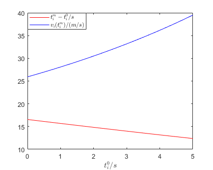
Numerical Example: We have also conducted simulations in MATLAB to study the solution of (65). The simulation parameters are $t_{i}^{0}=1s,v_{i}^{0}=20m/s,v_{i-1}(t_{i-1}^{m})=30m/s,t_{i-1}^{m}=15s,\varphi=1.8,\delta=0,L=400m,\beta=2.667$ ( $\alpha=0.2573$ ). Similarly as (19), we can still get four, six or eight solutions depending on these parameters. There is also only one feasible solution, i.e., $t_{i}^{m}=16.6856s$ .

In this case, $t_{i}^{0},v_{i}^{0}$ and $\beta$ will all affect the solutions. The simulation for the variation of $t_{i}^{0}$ is shown in Fig.11 ( $v_{i}^{0}=20m/s,v_{i-1}(t_{i-1}^{m})=30m/s,t_{i-1}^{m}=15s,\varphi=1.8,L=400m,\beta=2.667(\alpha=0.2573)$ ), the simulation for the variation of $v_{i}^{0}$ is shown in Fig.12 ( $t_{i}^{0}=1s,v_{i-1}(t_{i-1}^{m})=30m/s,t_{i-1}^{m}=15s,\varphi=1.8,L=400m,\beta=2.667(\alpha=0.2573)$ ), and the simulation for the variation of $\beta$ is shown in Fig.13 ( $t_{i}^{0}=1s,v_{i}^{0}=20m/s,v_{i-1}(t_{i-1}^{m})=30m/s,t_{i-1}^{m}=15s,\varphi=1.8,L=400m$ ).

We notice from Fig.12 and Fig.13 that the variation of $v_{i}^{0}$ and $\beta$ have few influence on the travel time $t_{i}^{m}-t_{i}^{0}$ , which is due to the safe merging constraint (4).

If we want the speed of the vehicle $i$ to be equal to the speed of the vehicle $i-1$ , i.e., $v_{i}(t_{i}^{m})=v_{i-1}(t_{i-1}^{m})$ , we can either put constraint on $t_{i}^{0}$ or $v_{i}^{0}$ . For example, we can make $v_{i}(t_{i}^{m})=v_{i-1}(t_{i-1}^{m})$ be a new constraint and take $v_{i}^{0}$ as a variable, then we can solve (65) together with this new constraint. In the simulation, $t_{i}^{0}=1s,v_{i-1}(t_{i-1}^{m})=30m/s,t_{i-1}^{m}=15s,\varphi=1.8,\delta=0,L=400m,\beta=2.667(\alpha=0.2573)$ . After solving these six nonlinear equations ,we can get $v_{i}^{0}=16.2005m/s,v_{i}(t_{i}^{m})=30m/s,t_{i}^{m}-t_{i}^{0}=15.8s$ . We can also check for the state constraint and control constraint with the solutions.

Following from Theorem 1, we have the following theorem for $i-1$ and $i$ :

Theorem 4: Under Assumptions 1-2, if CAVs $i$ and $i-1$ satisfy $v_{i}^{0}\leq v_{i-1}^{0}$ and $t_{i}^{0}-t_{i-1}^{0}\geq\varphi+\frac{\delta}{v_{i}^{0}}$ , then, under optimal control (15) for both CAVs, the safe merging constraint (4) is satisfied.

Remark 3: Theorem 4 is useful for the case that the vehicle $i$ arrives much later than $i-1$ , i.e., $t_{i}^{0}>>t_{i-1}^{0}$ . In this case, if we still use the optimal control solved by (65), the constraint (5) will most probably be violated. If Theorem 4 does not apply, we can also apply (15) for $i$ and check whether the safe merging constraint (4) will be satisfied or not. If yes, then we are done; otherwise, we can use the optimal control solved by (65).

III-B2 Safety Constraint Active

Suppose that the safety constraint between CAVs $i$ and $i_{p}$ becomes active at time $t_{1}\in(t_{i}^{0},t_{i}^{m})$ (where $t_{1}$ will be optimally determined), i.e., $g_{i}(t_{1})=0$ with $g_{i}(t_{1})$ defined in (42). As in section A, we can obtain the same optimal solutions as (44)-(45) for $t\geq t_{1}$ and the same optimal solutions as (52) for $t\in[t_{i}^{0},t_{1})$ , and Theorem 3 still holds.

In this case, we can always find an exit time $t_{2}$ from the safety constrained arc on an optimal trajectory because this safe merging constraint between $i$ and $i-1$ should be satisfied at $t_{i}^{m}$ . Starting from $t_{1}$ , we can apply the optimal control derived from (65) but with different intial conditions. As in Sec.III-A2, the safety constraint may be immediately violated, so we can obtain $t_{2}$ by solving

		$\displaystyle\frac{1}{2}a_{i}t_{2}^{2}+b_{i}t_{2}+c_{i}=v_{i}^{*}(t_{2}),$		(66)
		$\displaystyle\frac{1}{6}a_{i}t_{2}^{3}+\frac{1}{2}b_{i}t_{2}^{2}+c_{i}t_{2}+d_{i}=x_{i}^{*}(t_{2}),$
		$\displaystyle\frac{1}{6}a_{i}\cdot(t_{i}^{m})^{3}+\frac{1}{2}b_{i}\cdot(t_{i}^{m})^{2}+c_{i}t_{i}^{m}+d_{i}=L,$
		$\displaystyle v_{i-1}(t_{i-1}^{m})(t_{i}^{m}\!-\!t_{i-1}^{m})\!=\!\varphi(\frac{1}{2}a_{i}\cdot(t_{i}^{m})^{2}\!+\!b_{i}t_{i}^{m}\!+\!c_{i})\!+\!\delta$
		$\displaystyle\beta+0.5a_{i}^{2}\cdot(t_{i}^{m})^{2}+a_{i}b_{i}t_{i}^{m}+a_{i}c_{i}-0.5(a_{i}t_{i}^{m}+b_{i})^{2}$
		$\displaystyle+\frac{1}{\varphi}(a_{i}t_{i}^{m}+b_{i})v_{i-1}(t_{i-1}^{m})=0,$
		$\displaystyle a_{i}t_{2}+b_{i}=u_{i}^{*}(t_{2}).$

with $t_{1}$ to be optimally determined, where $x_{i}^{\ast}(t_{2}),v_{i}^{\ast}(t_{2})$ and $u_{i}^{\ast}(t_{2})$ are optimal solutions from (45). $t_{2}$ is a function of $t_{1}$ when solving (66).

We can still apply Theorem 2 to find the infeasible interval $I_{i}$ for $i$ to exclude these $t_{1}$ that do not make $t_{1}$ be the first time that the safety constraint (3) becomes active.

Therefore, we can apply (52) for $t\in[t_{i}^{0},t_{1})$ , apply (44) for $t\in[t_{1},t_{2})$ and apply the optimal control solved by (66) for $t\in[t_{2},t_{i}^{m}]$ . Then we can get the optimal solutions for $J_{i}^{*}(t_{1})$ ,

	$\displaystyle J_{i}^{}(t_{1})=\beta(t_{i}^{m}-t_{i}^{0})+\int_{t_{0}}^{t_{1}}\frac{1}{2}(u_{i}^{}(t))^{2}dt$		(67)
	$\displaystyle+\int_{t_{1}}^{t_{2}}\frac{1}{2}(u_{i}^{}(t))^{2}dt+\int_{t_{2}}^{t_{i}^{m}}\frac{1}{2}(u_{i}^{}(t))^{2}dt$		(67)

The optimal solution for $t_{1}$ is obtained by finding $t_{1}$ that minimizes $J_{i}^{\ast}(t_{1})$ . By (66), it follows that $t_{i}^{m}$ is dependent on $t_{1}$ .

We can also summarize the method of finding the optimal $t_{1}^{*}$ , $t_{2}^{*}$ , $x_{i}^{*}(t),v_{i}^{*}(t)$ and $u_{i}^{*}(t)$ by the following algorithm:

Algorithm 2 Safety constrained optimal trajectory,

i_{p}>i-1

Input: $t_{i}^{0},v_{i}^{0},x_{i_{p}}^{*}(t),v_{i_{p}}^{*}(t),u_{i_{p}}^{*}(t)$ ,
$x_{i-1}^{*}(t),v_{i-1}^{*}(t),u_{i-1}^{*}(t)$
Output: $t_{1}^{*},x_{i}^{*}(t),v_{i}^{*}(t),u_{i}^{*}(t)$ , $t_{2}^{*}$

1: solve (55)

2: if CAV

i_{p}

is under unconstrained optimal control (15) then

I_{i}:=\{t_{1}\in(t_{i}^{0},t_{i}^{m}]|u_{i}(t_{1})+\varphi a_{i}>u_{i_{p}}^{*}(t_{1})\}

4: else

I_{i}=\{t_{1}\in(t_{i}^{0},t_{i}^{m}]|\exists t\in[t_{i}^{0},t_{1}),g_{i}(t)>0\}

6: get feasible set

F_{i}:=(t_{i}^{0},t_{i}^{m})\setminus I_{i}

for

t_{1}

7: solve (53) and (66)

8: get

J_{i}^{*}(t_{1})

by (67)

9: solve for

t_{1}^{*}

over

F_{i}

(and

t_{2}^{*}

)

10: result =

t_{1}^{*},x_{i}^{*}(t),v_{i}^{*}(t),u_{i}^{*}(t),t_{2}^{*}

11: return result

Numerical Example: There three vehicles $i\in S(t)$ , $i_{p}(\neq i-1)\in S(t)$ and $i-1\in S(t)$ with parameters $t_{i_{p}}^{0}=0s$ , $v_{i_{p}}^{0}=20m/s,$ $t_{i-1}^{0}=0.1s,v_{i-1}^{0}=20m/s$ , $t_{i}^{0}=2.55s,v_{i}^{0}=28m/s$ let $\varphi=1.8s,,\delta=0m,L=400m$ , and $\beta=2.667$ ( $\alpha=0.2573$ ). The vehicle $i_{p}$ and $i$ are in the same lane, the vehicle $i-1$ is in the different lane with respect to $i_{p}$ and $i$ . Therefore, $i_{p}=i-2$ in the FIFO queue.

If we apply the optimal controller for $i_{p}$ solved by (19), the optimal controller for $i-1$ and $i$ solved by (65), then we can get their safety constraint and safe merging profile, as shown in Fig.14.

The safe merging constraint between $i-1$ and $i_{p}$ , $i-1$ and $i$ should only be satisfied at the merging point, as shown in Fig.14 (green and red lines). However, the safety constraint between $i_{p}$ and $i$ should always be satisfied. We notice the safety constraint between $i_{p}$ and $i$ is violated for some time, as shown in the second frame of Fig.14 (blue line). Therefore, we need to solve the optimal solution again. We use (52) for $t\in[t_{i}^{0},t_{1})$ , (53) for $t\in[t_{1},t_{2})$ and the optimal solution by (66) for $t\in[t_{2},t_{i}^{m}]$ . Firstly, we check whether there is infeasible interval $I_{i}$ for $t_{1}$ , as shown in Fig.15.

It follows from Fig.15 that the infeasible interval $I_{i}=(6.84,t_{i}^{m}]$ does exist in this case. The optimal objective function with respect to $t_{1}$ is shown in Fig.16 and we get $t_{1}^{\ast}=5.30s$ following from Fig.16.

We continue to study the state and safety constraint profiles at $t_{1}^{\ast}=5.30s$ and $t_{2}^{\ast}=5.5794s$ , as shown in Fig.17-20.

IV SIMULATION EXAMPLES

We have used the Vissim microscopic multi-model traffic flow simulation tool as a baseline to compare with the optimal control approach we have developed. The car following model in Vissim is based on [20] and simulates human psycho-physiological driving behavior.

The simulation parameters used are as follows: $L=400m,$ $\varphi=1.8,$ $\delta=0,$ $v_{max}=30m/s,$ $v_{min}=10m/s,$ $u_{max}=3.924m/s^{2}$ and $u_{min}=-3.924m/s^{2}$ . The simulation under optimal control is conducted in MATLAB by using the same vehicle input and initial conditions as in Vissim. The CAVs arrive randomly with 600 CAVs per hour arrival rate for both lanes.

The simulation results regarding the performance under optimal control compared to that in Vissim are summarized in Table I. We can see that the objective function defined in (6) is significantly improved under optimal control compared to the Vissim simulation for both cases ( $\alpha=0.26$ and $\alpha=0.41$ ). The same applies to the average travel times.

TABLE I: Objective function comparison

Items	OC		Vissim
Weight	$\alpha$ =0.26	$\alpha$ =0.41	$\alpha$ =0.26	$\alpha$ =0.41
Ave. time/s	17.0901	15.2297	30.9451
Main time/s	17.1304	15.2609	23.7826
Merg. time/s	17.0489	15.1978	38.2667
Ave. $\frac{1}{2}u_{i}^{2}(t)$	5.6979	11.9167	20.0918
Main $\frac{1}{2}u_{i}^{2}(t)$	5.8349	12.3077	9.4066
Merg. $\frac{1}{2}u_{i}^{2}(t)$	5.5580	11.5171	31.0144
Ave. obj.	38.4308	55.1110	76.8200	109.5478
Main obj.	38.6219	55.4402	54.5736	80.6316
Merg. obj.	38.2448	54.7745	99.5606	139.1065

Recognizing that $1/2u^{2}(t)$ is only an approximation of the actual fuel consumption of a vehicle, we have used the polynomial metamodel proposed in [4] for a more accurate evaluation of fuel consumption as a function of both $v_{i}(t)$ and acceleration $u_{i}(t)$ . This model is defined as

\dot{f}_{v}(t)=\dot{f}_{cruise}(t)+\dot{f}_{accel}(t)

(68)

where

\dot{f}_{cruise}(t)=\omega_{0}+\omega_{1}v_{i}(t)+\omega_{2}v_{i}^{2}(t)+\omega_{3}v_{i}^{3}(t)

\dot{f}_{accel}(t)=(r_{0}+r_{1}v_{i}(t)+r_{2}v_{i}^{2}(t))u_{i}(t)

and $\omega_{0}$ , $\omega_{1}$ , $\omega_{2}$ , $\omega_{3}$ , $r_{0}$ , $r_{1}$ and $r_{2}$ are positive coefficients (we used the values reported in [4]). It is assumed that during braking from a high velocity when $u_{i}(t)<0$ , no fuel is consumed. The comparison results are shown in Table II. As is to be expected, fuel consumption under optimal control is larger compared to that obtained in the Vissim simulation, since the form used for the objective function in (6) is different from (68). It remains unclear what an accurate fuel consumption model is and this is the subject of ongoing and future work aiming at appropriate modifications of (6).

TABLE II: Fuel consumption comparison

Items	OC ( $\alpha$ =0.26)	OC ( $\alpha$ =0.41)	Vissim
Ave. fuel/mL	48.6124	68.3194	36.9954
Main fuel/mL	48.0726	67.2866	42.6925
Merg. fuel/mL	49.1642	69.3752	31.1717

V CONCLUSIONS

We have derived a decentralized optimal control solution for the traffic merging problem that jointly minimizes the travel time and energy consumption of each CAV and guarantees that a speed-dependent safety constraint is always satisfied. Under certain simple-to-check condition in Theorems 1,4, we have shown that the safety constraint remains inactive and computation is simplified. Otherwise, we have still derived a complete solution that may include one or more arcs where the safety constraint is active. We have not taken into account speed and acceleration constraints for each CAV, which will be incorporated in future work by including appropriate arcs in the optimal trajectory as in [25]. Ongoing research is exploring the use of approximate solutions (e.g., the use of control barrier functions) as an alternative to an optimal control solution if the latter becomes computationally burdensome or if the use of more complex objective functions or more elaborate vehicle dynamics makes an optimal control approach prohibitive. Lastly, we will investigate the case where only a fraction of the traffic consists of CAVs, similar to the study in [23].

References

[1] Bryson and Ho. Applied Optimal Control. Ginn Blaisdell, Waltham, MA, 1969.
[2] W. Cao, M. Mukai, and T. Kawabe. Cooperative vehicle path generation during merging using model predictive control with real-time optimization. Control Engineering Practice, 34:98–105, 2015.
[3] W. Chen, Z. Zhao, Z. liu, and Peter C. Y. Chen. A novel assistive on-ramp merging control system for dense traffic management. In Proc. IEEE Conference on Industrial Electronics and Applications, pp. 386–390, Siem Reap, 2017.
[4] M. Kamal, M. Mukai, J. Murata, and T. Kawabe. Model predictive control of vehicles on urban roads for improved fuel economy. IEEE Transactions on Control Systems Technology, 21(3):831–841, 2013.
[5] W. Levine and M. Athans. On the optimal error regulation of a string of moving vehicles. IEEE Transactions on Automatic Control, 11(13):355–361, 1966.
[6] A. A. Malikopoulos, C. G. Cassandras, and Yue J. Zhang. A decentralized energy-optimal control framework for connected and automated vehicles at signal-free intersections. Automatica, 2018(93):244–256, 2018.
[7] V. Milanes, J. Godoy, J. Villagra, and J. Perez. Automated on-ramp merging system for congested traffic situations. IEEE Transactions on Intelligent Transportation Systems, 12(2):500–508, 2012.
[8] M. Mukai, H. Natori, and M. Fujita. Model predictive control with a mixed integer programming for merging path generation on motor way. In Proc. IEEE Conference on Control Technology and Applications, pp. 2214–2219, Mauna Lani, 2017.
[9] I. A. Ntousakis, I. K. Nikolos, and M. Papageorgiou. Optimal vehicle trajectory planning in the context of cooperative merging on highways. Transportation Research, 71, Part C:464–488, 2016.
[10] G. Raravi, V. Shingde, K. Ramamritham, and J. Bharadia. Merge algorithms for intelligent vehicles. In: Sampath, P., Ramesh, S. (Eds.), Next Generation Design and Verification Methodologies for Distributed Embedded Control Systems. Springer, Waltham, MA, 2007.
[11] C. Rathgeber, F. Winkler, X. Kang, and S. Muller. Optimal trajectories for highly automated driving. International Journal of Mechanical, Aerospace, Industrial, Mechatronic and Manufacturing Engineering, 9(6):946–952, 2015.
[12] J. Rios-Torres, A.A. Malikopoulos, and P. Pisu. Online optimal control of connected vehicles for efficient traffic flow at merging roads. In Proc. IEEE 18th International Conference on Intelligent Transportation Systems, pp. 2432–2437, Las Palmas, Spain, 2015.
[13] R. Scarinci and B. Heydecker. Control concepts for facilitating motorway on-ramp merging using intelligent vehicles. Transport Reviews, 34(6):775–797, 2014.
[14] B. Schrank, B. Eisele, T. Lomax, and J. Bak. The 2015 urban mobility scorecard. Texas A&M Transportation Institute, 2015.
[15] M. Tideman, M.C. van der Voort, B. van Arem, and F. Tillema. A review of lateral driver support systems. In Proc. IEEE Intelligent Transportation Systems Conference, pp. 992–999, Seatle, 2007.
[16] P. Varaiya. Smart cars on smart roads: problems of control. IEEE Transactions on Automatic Control, 38(2):195–207, 1993.
[17] K. Vogel. A comparison of headway and time to collision as safety indicators. Accident Analysis & Prevention, 35(3):427–433, 2003.
[18] D. De Waard, C. Dijksterhuis, and K. A. Broohuis. Merging into heavy motorway traffic by young and elderly drivers. Accident Analysis and Prevention, 41(3):588–597, 2009.
[19] J. Weng, S. Xue, and X. Yan. Modeling vehicle merging behavior in work zone merging areas during the merging inplementation period. IEEE Transactions on Intelligent Transportation Systems, 17(4):917–925, 2016.
[20] R. Wiedemann. Simulation des straßenverkehrsflusses. In Proc. of the Schriftenreihe des tnstituts fir Verkehrswesen der Universitiit Karlsruhe (In German language), 1974.
[21] X. Zang. The short-term traffic volume forecasting for urban interchange based on rbf artificial neural networks. In Proc. IEEE Conference on Mechatronics and Automation, pp. 2607–2611, Changchun, 2009.
[22] Yue J. Zhang and C. G. Cassandras. A decentralized optimal control framework for connected automated vehicles at urban intersections with dynamic resequencing. In Proc. 57th IEEE Conference on Decision and Control, 2018. To appear.
[23] Yue J. Zhang and C. G. Cassandras. The penetration effect of connected automated vehicles in urban traffic: an energy impact study. In Proc. 2018 IEEE Conference on Control Technology and Applications, pp. 620–625, Copenhagen, Denmark, 2018.
[24] Yue J. Zhang, C. G. Cassandras, and A. A. Malikopoulos. Optimal control of connected and automated vehicles at urban traffic intersections: A feasibility enforcement analysis. In Proc. of the American Control Conference, pp. 3548–3553, Seattle, 2017.
[25] Yue J. Zhang, A. A. Malikopoulos, and C. G. Cassandras. Optimal control and coordination of connected and automated vehicles at urban traffic intersections. In Proc. of the American Control Conference, pp. 6227–6232, Boston, 2016.

		$\displaystyle x_{i}^{}(t)=\left\{\!\begin{array}[]{lcl}\begin{aligned} &-c_{v_{1}}\varphi e^{-\frac{1}{\varphi}t}+x_{i_{p}}^{}(t)-d_{i_{p}}-\\ &\varphi(v_{i_{p}}^{}(t)-c_{i_{p}})+a_{i_{p}}\varphi^{2}t+c_{x_{1}}\end{aligned}&t\in[t_{1},t_{i_{p}}^{m}]\\ -c_{v_{2}}\varphi e^{-\frac{1}{\varphi}t}+v_{i_{p}}^{}(t_{i_{p}}^{m})t+c_{x_{2}}&t\in(t_{i_{p}}^{m},t_{i}^{m}]\end{array}\right.$		(53)
		$\displaystyle v_{i}^{}(t)=\left\{\!\begin{array}[]{lcl}c_{v_{1}}e^{-\frac{1}{\varphi}t}\!+\!v_{i_{p}}^{}(t)\!-\!\varphi u_{i_{p}}^{}(t)\!+\!a_{i_{p}}\varphi^{2}&t\in[t_{1},t_{i_{p}}^{m}]\\ c_{v_{2}}e^{-\frac{1}{\varphi}t}+v_{i_{p}}^{}(t_{i_{p}}^{m})&t\in(t_{i_{p}}^{m},t_{i}^{m}]\end{array}\right.$
		$\displaystyle u_{i}^{}(t)=\left\{\begin{array}[]{lcl}-\frac{c_{v_{1}}}{\varphi}e^{-\frac{1}{\varphi}t}+u_{i_{p}}^{}(t)-\varphi a_{i_{p}}&t\in[t_{1},t_{i_{p}}^{m}]\\ -\frac{c_{v_{2}}}{\varphi}e^{-\frac{1}{\varphi}t}&t\in(t_{i_{p}}^{m},t_{i}^{m}]\end{array}\right.$

Decentralized Optimal Merging Control for Connected and Automated Vehicles

Abstract

I INTRODUCTION

II PROBLEM FORMULATION

III DECENTRALIZED FRAMEWORK

III-A Decentralized Optimal Control when i−1=ipi-1=i_{p}

III-A1 Control, state, safety constraints not active

III-A2 Safety Constraint Active

III-B Decentralized Optimal Control when i−1>ipi-1>i_{p}

III-B1 Control, state, safety constraints not active

III-B2 Safety Constraint Active

IV SIMULATION EXAMPLES

V CONCLUSIONS

References

III-A Decentralized Optimal Control when $i-1=i_{p}$

III-B Decentralized Optimal Control when $i-1>i_{p}$