A new universal ratio in Random Matrix Theory and chaotic to integrable transition in Type-I and Type-II hybrid Sachdev-Ye-Kitaev models
Abstract
We investigate chaotic to integrable transition in two types of hybrid SYK models which contain both SYK with interaction and SYK with an interaction in type-I or SYK with an interaction in type-II. These models include hybrid Majorana fermion, complex fermion and bosonic SYK. For the Majorana fermion case, we discuss both even and odd case. We make exact symmetry analysis on the possible symmetry class of both types of hybrid SYK in the 10 fold way by Random Matrix Theory (RMT) and also work out the degeneracy of each energy levels. We introduce a new universal ratio which is the ratio of the next nearest neighbour (NNN) energy level spacing to characterize the RMT. We perform exact diagonalization to evaluate both the known NN ratio and the new NNN ratio, then use both ratios to study Chaotic to Integrable transitions (CIT) in both types of hybrid SYK models. Some preliminary results on possible quantum analog of Kolmogorov-Arnold-Moser (KAM) theorem and its dual version in the quantum chaotic side are given. We explore some intrinsic connections between the two complementary approaches to quantum chaos: the RMT and the Lyapunov exponent by the expansion in the large limit at a suitable temperature range. We stress the crucial differences between the quantum phase transition (QPT) characterized by renormalization groups at , expansions at a finite and the CIT characterized by the RMT at a finite : the former focus on the ground state and its low energy excitations ( edge states in the Fock space ), the latter on excited states ( bulk states in the Fock space ). We also discuss Eigenstate Thermalization hypothesis (ETH)’s power on a quantum chaotic bulk state and its inability to encode the edge states. Comments on some previously related works are given. Some future perspectives, especially the failure of the Zamoloddchikov’s c-theorem in 1d CFT RG flow are outlined.
I Introduction
In classical chaos, the Lyapunov exponent was used to characterize the exponential growth of two classical trajectories when there are just a tiny difference in the initial conditions. The classical concept of Lyapunov exponent can be extended to its quantum analog to characterize the exponential growth of two initially commuting operators in the early time (up to the Ehrenfest time) under the evolution of a quantum chaotic Hamiltonian [1, 2, 3]. There are recent flurry of research activities to extract the Lyapunov exponent of the Sachdev-Ye-Kitaev (SYK) model and its various variants through evaluating out of time ordered correlation (OTOC) functions [4, 5, 6, 7, 8, 9, 10, 11, 12, 13, 14, 15]. The quantum analog of need to be evaluated away from the thermodynamic limit by a expansion in the SYK models, also away from the conformal invariant limit due to a leading irrelevant operator and at a finite temperature (ranging from low to infinite temperatures). There are also calculations in the dual bulk quantum black holes in an asymptotic geometry to demonstrate the correspondence between the SYK models and Jackiw-Teitelboim gravity [16, 17, 18, 19]. The quantum chaos in the SYK models are due to the quenched disorders and interactions. However, it inspired a new class of clean models called (colored or un-colored) Tensor (Gurau-Witten) model [30, 31, 32], which share similar quantum chaotic properties as the SYK models at least in the large limit.
From a completely different perspective and also at a much longer time scale ( Heisenberg time ), the quantum chaos can also be characterized by the system’s energy level-level correlations encoded in the energy level statistics (ELS) and the spectral form factor (SFF) through random matrix theory (RMT)[20, 21, 22]. The ELS and SFF are always evaluated in a finite but sufficiently large system [23, 24, 25, 26, 27]. The ELS of SYK can be described by the Wigner-Dyson (WD) distributions in a way [23, 24, 25, 29]: Gaussian unitary ensembles (GUE), Gaussian orthogonal ensemble (GOE), Gaussian symplectic ensemble (GSE).
Here we investigate chaotic to integrable transitions (CIT) in two types of hybrid SYK models. The type-I contains both the chaotic SYK with interaction and the integrable SYK with interaction . It violates the particle-hole (PH) symmetry and includes the hybrid Majorana fermion, complex fermion and hard-core bosonic SYK. The type-II includes SYK of either Majorana or complex fermion with interaction and SYK with the interaction . It preserves the particle-hole (PH) symmetry. In this work, we mainly use the RMT approach, but will also explore some possible connections between the RMT approach and the Lyapunov exponent which can be extracted from the out of time correlation functions (OTOC).
There are direct motivations to study both types of Hybrid SYK models. It was also known that the SYK model provides a concrete model to realize Eigen-state Thermalization Hypothesis (ETH) [43]. Even the entanglement entropy of its ground state satisfies the volume law instead of the more common area law. Here it is important to study how the gapless quantum spin liquid (QSL) responses under the Type I or Type II kinds of integrable perturbations. It would also be interesting to study how the ETH breaks down under the Type I or Type II kind of integrable perturbations. On the dual bulk gravity side, these kind of perturbations are also needed to probe the interior behind the black hole horizon [45]. Most importantly, in any possible experimental systems to realize SYK models, the Type I and Type II terms are most common perturbations. As shown in Fig.9 in the conclusion section, the two types hybrid SYK models also provide specific examples of RG flow between two CFT1 fixed points which violate Zamoloddchikov’s c-theorem. When comparing with some previously studied hybrid models, one can see there are also many other motivations to study both types of hybrid SYK models. For example, the multi-channel Kondo models show non-Fermi liquid (NFL) behaviours, so it is important to study how the NFL changes under spin or channel anisotropy [36, 38, 39, 40]. The Kitaev honeycomb lattice model [41] hosts a Majorana fermion quantum spin liquid (QSL), so it is important to study how the Majorana fermion QSL changes under adding other interactions such as a Heisenberg interaction or a Dzyaloshinskii-Moriya (DM) term [42].
We first introduce a new universal ratio which is the ratio of next nearest neighbor (NNN) energy spacing to characterize the RMT classes and also establish its relations with the well-known ratio of the nearest neighbor (NN) energy spacing [46]. When a doubly degenerate level is split by a small perturbation, the NN ratio is nearly zero and also rapidly changing, the new NNN ratio can be used to effectively characterize the “hidden” RMT behaviours, especially the CIT. We make exact symmetry analysis to classify the possible symmetry class in the 10-fold way[29, 47, 50], and then perform exact diagonalization (ED) on all these hybrid models. In the Majorana fermion case, we pay special efforts to classify the odd case. Both the NN ratio and the NNN ratio are evaluated when a doubly degenerate level is split by a small perturbation. In the type-I hybrid SYK, as increases, there is always a chaotic to integrable transition (CIT) from GUE to Poisson in all the hybrid Majorana or complex fermionic models, but not the hybrid bosonic model. Starting from the type-I hybrid Majorana or complex fermion SYK side, for the GOE case, there is a GOE to GUE crossover first, then a CIT from the GUE to the Poisson; for the GUE case, there is a direct CIT from the GUE to the Poisson; for the GSE case, any small destroys the double degeneracy of the GSE, the NN ratio rises to GUE, then a CIT from the GUE to the Poisson. In this case, the NNN ratio can be most effectively applied to describe the stability regime of GSE near the chaotic side and may also be used to describe the whole crossover until to the integrable side.
In the type-II hybrid SYK, the symmetry analysis alone may not be able to distinguish between the chaotic SYK and integrable SYK. As increases, there are always CIT from the corresponding WD distribution dictated by the symmetry of the SYK to the Poisson controlled by the SYK. When there is a double degeneracy at the side, the NNN can be most effectively applied to describe the CIT and may also be used to describe the whole crossover until to the quantum chaotic side.
In classical chaos, the classical Kolmogorov-Arnold-Moser (KAM) theorem states that if an integrable Hamiltonian is disturbed by a small perturbation , which makes the total Hamiltonian non-integrable. If the two conditions are satisfied: (a) is sufficiently small (b) the frequencies of are in-commensurate, then the system remains quasi-integrable. Despite some previous efforts, the quantum analogue of the KAM theorem remains elusive. Just like the quantum analog of Lyapunov exponent can be studied in the context of the SYK models [4, 5, 6, 7, 8, 9, 10, 11, 12, 13, 16, 14, 15], it is important to explore the quantum analog of KAM theorem in both types of hybrid SYK models. We first give a definition of the quantum analogue of the KAM theorem and also its possible dual form which is the stability of quantum chaos in the context of RMT. Then we use both NN and NNN ratio to numerically characterize the KAM regime in the integrable side and the stability of quantum chaos in the chaotic side. We give some preliminary results on possible quantum analog of the KAM theorem, the stability of quantum chaos ( can also be called the dual form of the KAM theorem ), especially its dependence on the system’s size in the two types hybrid SYK models. By pushing the methods developed in [70] further, we leave rigorous mathematical treatments to a future publication [71].
We also stress the crucial differences between the onset of quantum phase transitions (QPT) at characterized by renormalization group (RG), expansions and the onset of CIT characterized by the RMT at a finite . The former is focusing on the changes in the ground state and low energy excitations ( called edge excitations in the Fock space ), there is an associated divergent length scale and quantum critical scalings and a finite size scaling at a finite size. While the latter is focusing on the changes in the correlations in the bulk energy levels in the Fock space, there is no associated divergent length scale, therefore no quantum critical scalings and no finite size scaling at a finite size. We also discuss Eigenstate Thermalization hypothesis (ETH)’s power on a quantum chaotic bulk state and its inability to encode the ground state and low energy excitations. Some comments on previous works on type-I hybrid SYK models are given. Some perspectives and possible future directions are outlined in the conclusion section. Especially, we point out that the Zamoloddchikov’s c-theorem of 2d CFT and its extensions to 2d boundary CFT and higher dimensions break down in 1d CFT RG flow. This fact maybe related to may also be dramatically different than its high dimensional counterparts.
As mentioned in the first two paragraphs, there are two complementary approaches to describe the quantum chaos: the OTOC at an early time and the RMT at a later time. However, so far, it seems there is no clear connections between the two different ways to characterize the quantum chaos. In this work, we establish some intrinsic connections between the two approaches: the quantum chaos in the bulk energy levels described by the RMT implies the quantum information scramblings with a non-vanishing Lyapunov exponent by the OTOC in the edge levels ( the ground state and low energy levels ) in a suitable temperature range.
II A new ratio to describe RMT: ratio of next nearest neighbor energy spacing
In this section, we first review the known results on the statistics of the NN energy level spacing , then introduce a new ratio which is the NNN energy level spacing , then establish an approximate, but quite accurate relation between the two.
II.1 Review on the ELS of NN energy level spacings
Let be an ordered set of energy levels and are the NN spacings. By considering a matrices system, Wigner derived a simple approximate expression for the distribution function of the NN spacing,
| (1) |
where is the Dyson index for GOE, GUE and GSE respectively. It is also known that independent random energy levels would yield a Poisson distribution
| (2) |
However, in order to compare different results from different systems, the energy levels will need an unfolding procedure, which is not convenient when large enough statistics is not available To get rid of the dependence on the local density of states, it is convenient to look at the distribution of the ratio of two adjacent energy level spacings [46, 23] which distributes around . This quantity has the advantage that it requires no unfolding since ratios of consecutive level spacings are independent of the local density of states.
By considering matrices system, the authors in [46] obtained the Wigner-like surmises of the ratio of consecutive level spacings distribution
| (3) |
where and for GOE, GUE and GSE respectively. The distribution has the same level repulsion at small as , namely, . However, the large asymptotic behavior is dramatically different than the fast exponential decay of .
II.2 Introduction and calculation of the ELS of NNN energy level spacings
When there are nearly double degenerated energy levels, we find that it is convenient to introduce next nearest-neighbor (NNN) spacings and ratios . Here we study the distribution of the ratio of the two NNN spacings by exploring the exact calculation for matrices.
For a Poisson ensemble, it is more convenient to work with and the ratio of consecutive NNN level spacings is . The NNN ratio distribution can be calculated from
| (5) |
Since energy levels are not correlated in Poisson ensemble, one can rewrite and evaluate the integral to obtain a simple result
| (6) |
It is easy to see that when is small, and when is large. Interestingly, there is a NNN level repulsion in Poisson ensemble which intuitively can be understood due to the interruption of the intermediate level.
For various Gaussian ensembles, it is good to start from the joint probability distribution and the ratio of consecutive NNN level spacings is . The NNN ratio distribution can be calculated from
| (7) |
where the joint probability distribution takes the form . The integral can be simplified as
| (8) | ||||
where means the normalization constant is ignored. The integrals can be evaluated analytically, but its expression is lengthy. Here, we just show analytically its asymptotic behaviour: when is small, and when is large. If comparing them with those of , one can see that the asymptotic behaviours of the NNN level statistics with index are the same as those of the NN with index (See Eq.(10) below for all the ranges). Similar to the Poisson case discussed above, the intermediate energy level induces much stronger level repulsions between NNN. In Fig.1, we compare obtained from Eq.(8) against the numerical simulations of the corresponding WD ensembles. We find nearly perfect agreement in all ranges of .

It is easy to check that have the same symmetry as , namely, , thus we can still define a . From the NNN ratio distribution given in Eq.(6) for Poisson and Eq.(8) for WD, one can calculate expectation value for and as
| (9) |
which are listed in Table I.
| Ensembles | Poisson | GOE | GUE | GSE |
|---|---|---|---|---|
| 1.75 | 1.3607 | 1.1747 | ||
| 0.38629 | 0.5359 | 0.6027 | 0.6762 | |
| 2 | 1.1736 | 1.0972 | 1.0516 | |
| 0.5 | 0.6769 | 0.7344 | 0.7910 | |
| – | 1.1747 | 1.0980 | 1.0681 | |
| – | 0.6762 | 0.7335 | 0.7672 |
II.3 An approximate but accurate relation between the ELS of NNN and those of NN
In fact, instead of lengthy results from exact evaluation of integral, we find an approximate relation between and :
| (10) |
The difference of the two was shown in Fig.2. The very small deviation shows that the approximation in Eq.(10) is quite accurate. In the last two lines in the TABLE I, we also list the numerical values of and using . All these values are very close to those using in Eq.8. For example, just take for the GSE case, one can see the relative difference is very small.
In fact, one can see Eq.10 can also work well when putting . Namely, when the NN satisfies Poisson, the NNN seems fit GOE approximately. For example, from the TABLE I, and for Poisson are and which are not too much away from and for GOE ( and ). At least, one can use GOE for an quick eye guides to judge the NNN for the Poisson as we did in all the following figures.

.
In the following sections, we will apply both NN and NNN ELS to study the CIT in the two types of hybrid Sachdev-Ye-Kitaev models.
III Type-I Hybrid Sachdev-Ye-Kitaev models
By Type-I, we mean the integrable side is given by SYK which breaks the PH symmetry Eq.12 of the SYK. We will discuss Majorana and complex type-I hybrid SYK respectively.
III.1 The hybrid of and Majorana fermion SYK
The CIT may be first investigated in the hybrid of and Majorana fermion SYK, which also known as type-I hybrid Majorana SYK model:
| (11) |
where are real and satisfy the Gaussian distributions with and respectively. In the following, we denote the first term of , SYK model, as , and the second term, SYK model, as .
In the limit, the SYK breaks the PH symmetry Eq.12. It is non-interacting, so must be integrable. Its single particle density of state (DOS) satisfies the semi-circle law [11], while its many body ELS satisfies the Poisson distribution [9, 11, 25]. Its many body low or high energy excitation level spacing is , the low energy quasi-particle picture holds. Its entropy density vanishes. This is very similar to the Dicke model [64, 65, 66, 67, 68] in the limit (inside the superradiant phase) where the many body ELS also satisfies the Poisson distribution, and the low energy excitation level spacing is also where is the phase diffusion constant.
In the limit, the SYK Hamiltonian is non-integrable at any finite . In the following, we discuss when is even or odd respectively. For even number of sites , one can split the sites to even and odd, then introduce complex fermions[10, 23, 25] by and define the PH symmetry operator to be [52]
| (12) |
It is easy to show where . The total number of fermions . It is not a conserved quantity, but the parity is in . Then which justifies as an anti-unitary PH transformation. also commutes with the Hamiltonian [51] . Depending on , the ELS satisfies GUE when , GOE when , GSE when [10, 23, 25]. The ELS, the degeneracy at a given parity sector, and the total parity sector are listed in the Table IIa. Its low or high energy excitation level spacing is which leads to extensive entropy (in the limit before limit) [5, 7, 9]. The system’s many body DOS (different from the single particle DOS) has been worked out in [9] to be similar, but different than the semi-circle DOS. The quasi-particle picture completely breaks down. This is similar to the Dicke model in the limit (inside the superradiant phase) where the ELS satisfies the GOE distribution [67, 68] ( See Sec V-C ), its two lowest energy splitting between two opposite parities is which is due to the instanton quantum tunneling (QT) process. Of course, the ground state of SYK is a gapless quantum spin liquid. While that of Dicke model is a gapped symmetry broken super-radiant state at .


However, when is odd, the above procedures for even needs to be modified. In fact, one can still take the advantage of the above representation with even case by adding to make the parity conservation explicitly, but also enlarge the Hilbert space twice. Similar strategy was used before to study the symmetry protected topological phase of odd number of Majorana chain [56] and the ELS of the SYK model with odd [23, 53]. Then one can still define with as before. All the commutation relations still apply.
So when , is even, then respectively. Under , maps to the same parity sector. So it is in GSE and GOE with degeneracy and respectively at a given parity sector. When using the operator (see Eq.(13) below) which maps to , so it establishes the connection between the two parity sectors. So it has the degeneracy and when considering both parities.
When , is odd, then respectively. However, under , maps to the opposite sector . So one may only use to establish the connection between the two opposite parity sectors. This forced us to look for a new operator which may map into the same sector and still commutes with the Hamiltonian. This new operator is found to be:
| (13) |
which can be written down by just changing in to . So it will play a complementary role as which will be analyzed in the following.
One can show that where is excluded and the number is defined below Eq.12. It is also easy to see that . Using the fact that the Hamiltonian does not contain the fermions added at infinity, one can show that it still commutes with the Hamiltonian . It also leads to where .
So when , is odd. Under , maps to the same sector. and respectively, so it is in GOE and GSE with degeneracy and respectively at a given parity sector. When using the operator (see above) which maps to , so it establishes the connection between the two parity sectors. Then it has the degeneracy and when considering both parities.
| 0 | 2 | 4 | 6 | |
| ELS | GOE | GUE | GSE | GUE |
| 1 | 2 | 4 | 2 | |
| 1 | 3 | 5 | 7 | |
| ELS | GOE | GSE | GSE | GOE |
| 1 | 4 | 4 | 1 | |
Now we apply the PH transformation to the hybrid SYK model Eq.11. The parity remains to be conserved. However, ( when , one use , in all the other cases, one use ) is not conserved anymore due to (or ). So the hybrid SYK does not have the PH symmetry anymore. Just from symmetry point of view (the 10-fold way classification scheme), the hybrid Majorana SYK Eq.11 belongs to the class A, so may satisfy GUE for any ratio of . Our ED studies [57] at a given parity sector were shown in Fig.3 for even and 4 for odd . In the following, we will discuss them respectively.
For even , there are 3 cases: (a) For , the Majorana fermion SYK at is in GOE, the hybrid is in the GUE around to , there is a crossover from GOE to GUE first, then a CIT from GUE to the Poisson as increases.
(b) For , the Majorana fermion SYK at is in GUE, it stays in the GUE until , then there is a CIT from GUE to the Poisson as increases.
(c) For , the Majorana fermion SYK at is in GSE at . Because , any energy level is doubly degenerate at a given parity sector, so when doing ELS, we only pick up one of the doubly degenerate levels to demonstrate the GSE. Any small breaks the degeneracy, then we may consider both sets of energy levels, a small makes small, so starts from zero and increases as increases, then reaches the GUE in the range from to . There is a CIT from GUE to the Poisson as increases. So in this case, using the NN ELS is not enough. One may start to use the combination of NN and the NNN ELS presented in Sec.2. The was also shown in Fig.3d. It is convenient to combine both and into the same Fig.3d. When in (d) is close to be zero, the NNN in (d) still shows GSE until . When in (d) reaches the plateau value of GUE with , then according to Eq.10, in (d) reaches the corresponding plateau value listed in Table I as with a RMT index . When in (d) reaches the plateau value of Poisson, according to Eq.10, in (d) reaches a corresponding plateau value listed in Table I as . As pointed out in Sec.2, it is only slightly below the GOE value with the RMT index .
For odd , due to the absence of the GUE in Table IIb, at the side, there are only the GSE case in (a) and (d), the GOE case in (b) and (c). They show similar evolution patterns as the corresponding GSE and GOE cases at the side for even cases shown in Fig.3.
Obviously, at any given disorder realization of , the eigen-energies of SYK is in-commensurate (so the disorder in SYK may play a similar role as the Berry phase in the Dicke model), a quantum version of Kolmogorov-Arnold-Moser ( KAM ) theorem [68] ( See Sec V-C ) should apply when is sufficiently small ( See Sec V-C ). So the ELS changes from the Poisson to GUE around some critical values. The mean value also changes from its Poisson value to the corresponding GUE value. It is similar to the in the Dicke model where the ELS changes from the Poisson to GOE when inside the superradiant phase (see Fig.2a in [68]). Of course, in contrast to the Dicke model, due to the quenched disorders, there is no regular regime (see Fig.2b in [68]) at any values of . Compared to the ED to study the CIT in the Dicke model, the extra work needed here is that one need to draw the random couplings from the corresponding Gaussian distributions and , then get ELS at a given set of . Then one need to repeat the same calculations over 40 to 100 samples of such a random realizations of , then perform the average of ELS over these 40 to 100 samples [55].
One may also understand the quantum analog of the KAM theorem from a dual point of view, namely, the stability of quantum chaos of the quantum chaotic SYK against the non-chaotic perturbation as one turns on . The dual form of the KAM theorem states that as increases, there should be a crossover from the WD to the GUE, then a CIT from the GUE to the Poisson. Our ED studies shown in Fig.3 and 4 confirms this global picture.
III.2 The hybrid of and complex fermion SYK
The Majorana fermion SYK was extended to the complex fermion which has a charge symmetry [10]. One may also add a chemical potential to fix the conserved fermion filling factor [54]:
| (14) |
The procedures used for the Majorana fermion in the last subsection ( of course, no odd case anymore ) can also be applied to study the and type-I hybrid complex SYK:
| (15) |
where drawing from the Gaussian distribution where . In general, . We also take the four site indices are all different [60] to keep the PH symmetry explicit at . is a Hermitian matrix satisfying .

In the limit, the complex SYK is non-integrable at any finite . Under the PH transformation, . So is the PH symmetric and only happens when is even. At the half-filling , the system also has the maximum zero temperature entropy [10]. Away from the half-filling , it breaks the symmetry, corresponds to a non-vanishing electric field in a charged black hole in an asymptotic bulk [7]. It was shown in [23] that when , the ELS is GOE and GSE respectively. But when and , it is GUE. In fact, as long as , there is no PH symmetry anymore, so it is in GUE regardless of the value of .
Now we apply the PH transformation to the hybrid SYK model Eq.15 when . The fermion number remains to be conserved. However, is not conserved anymore due to ( here and thereafter, excludes in Eq.15 ). So the hybrid SYK does not have the PH symmetry anymore. Just from symmetry point of view, the hybrid complex SYK belongs to the class A in the 10 fold way classification, so may satisfy GUE for any ratio of . Our ED studies [57] at a given in Fig.5 shows that this is true only in the intermediate regimes of . The KAM theorem and its dual form applies in the two end regimes where the ELS remains Poisson and where the ELS becomes the WD determined by the SYK respectively.
In our ED studies [57], we first study SYK to reproduce the known results in [23], then look at the SYK to show that it indeed satisfies the Poisson distribution. Then we study the hybrid model Eq. 15 at a given at any . The ED result is shown in Fig.5 where there are also 3 cases:
(a) For , at the half filling , the hybrid complex fermion SYK is in the GUE in a wide range near , there is a crossover from GOE to GUE, then a CIT from GUE to the Poisson as increases.
(b) Away from the half filling , regardless of , the SYK is in GUE. The hybrid complex fermion SYK stays in the GUE across until to , then there is a CIT from GUE to the Poisson as increases further.
(c) For , at the half filling , the complex fermion SYK is in GSE at . Because , any energy level is doubly degenerate, so when doing ELS, we only pick up one of the doubly degenerate levels to demonstrate the GSE at . Any small breaks the degeneracy, then we may need to consider both sets of energy levels, then it is easy to see that any small makes small, so starts from zero and increases as increases. The hybrid complex fermion SYK is in the GUE in a wide range near . There is a CIT from GUE to the Poisson as increases further.
So in this case, using the NN ELS is not enough. One must to use the combination of NN and the NNN ELS presented in Sec.2. The was also shown in Fig.5c. It is complete to combine both and into the same figure. When is close to be zero, the NNN still shows GSE until . When reaches the plateau value of GUE with , then according to Eq.10, reaches an corresponding plateau value listed in Table I as with a RMT index . When reaches the plateau value of the Poisson, according to Eq.10, reaches an corresponding plateau value listed in Table I as . It is only slightly below the GOE value with the RMT index .
IV Type II hybrid SYK models
By Type-II, we mean the integrable side is given by SYK which keeps the PH symmetry Eq.12 of the SYK. We will discuss Majorana and complex type-II hybrid SYK respectively. The results can be contrasted with the corresponding Type-I hybrid SYK models.
IV.1 The particle-hole or conserving hybrid Majorana fermion SYK
It may also be interesting to study the CIT in the type-II hybrid Majorana fermion SYK which keeps the PH symmetry at any ratio of :
| (16) |
where , are real and satisfy the Gaussian distributions with , and , respectively. Note that here we use to make dimensionless.
Obviously, the second term of can be written as . In contrast to Eq.11, it still keeps the symmetry. So symmetry analysis alone can not distinguish between and despite the former is chaotic, the latter is integrable. Because is integrable, so is . This can be most conveniently seen from the NN ratio of the . Then of the can be written as:
| (17) |
where, similar to the cancelation of the density of states in , the center of two NN energies just cancels in the ratio. Very similarly, one can show that the ratio of the NNN energy spacing . So the ELS of remains Poisson.
This model with both sign was studied before in [23] by expansion and by the RG analysis at . By performing the RG on the coefficient of the term around the SYK conformally invariant fixed point, it was found that the sign is marginally irrelevant (Fig.9b2), so the non-integrable SYK NFL fixed point is stable in the IR against the perturbation. However, the is marginally relevant (Fig.9b1), it flows to the integrable FL fixed point controlled by . However, our ED results show that there is very little differences between the two signs in ELS. This fact could be explained as follows:
| (18) |
where . So and satisfy the same distribution.


Let be an ordered set of energy levels of , then are the NN spacings. Then is the corresponding ordered set of energy levels of and are the corresponding NN spacings. Similarly, the NNN spacing . Because and satisfy the same distribution, so we conclude satisfy the same ELS. [59]. This is confirmed by our ED. So we just show our sign results in Fig.6 and 7. However, there is an exchange between the ground state and the highest energy state in the sign, so the will have completely different ground states. This can also be seen by the RG analysis in Fig.9b1,b2 [23]. This fact may show that the CIT characterized by the RMT at a finite may be complementary to the QPT characterized by the RG at . Further elucidations on the intricate relation between RG and RMT will be given in Sec. V.
Because or ( when , one use , in all the other cases, one use ), so symmetry analysis alone can not distinguish between and . So the symmetry classification in Sec.3 still applies to this Type-II hybrid Majorana fermion SYK at any . So the Table II still holds. Our ED studies [57] in Fig.6 and 7 shows that this is true up to . Then the KAM theorem applies at small where the ELS becomes Poissonian. There is a CIT from the corresponding WD to the Poisson as increases. However, the degeneracy in Table I remains true at any . In the following, we discuss even and odd case respectively.
For even shown in Fig.6, there is always a CIT from the corresponding WD to the Poisson. Several salient features need to be stressed. For in (b), one may also look at the ELS from the side when . Because , then are still in the same parity sector, but have two different eigenvalues , so are orthogonal. But , a pair of orthogonal eigenstates have the same eigenvalue . So is doubly degenerate at . However, the double degeneracy is broken by any . Then using the NN ELS is not enough. One must use the combination of NN and the NNN ELS presented in Sec.2. In contrast to all the previous cases with or violating Type-I hybrid SYK models where the doubly degeneracy comes from the non-integrable side, here the doubly degeneracy comes from the integrable side. It is best to combine and in Fig.6b and read them from the integrable side. When is close to be zero, the NNN still shows Poisson until . When reaches the plateau value of the GOE with , then according to Eq.10, reaches an corresponding plateau value listed in Table I as which is quite close to GSE with a RMT index .
For in (d), there is a CIT from GSE to Poisson as increases. As shown in Table II, there is always a double degeneracy at any . Although in (b) is quite similar to in (d), both of which looks like to show a CIT from GSE to Poisson, they have very different physical meanings. As said above, with in (b) represents NNN ELS, so it stands for a CIT from GOE to Poisson. While with in (d) represents NN ELS, so it is a true CIT from GSE to Poisson.
For in (c) and (a), there is no degeneracy at any . There is a CIT from GUE to Poisson as increases.
The odd case is shown in Fig.7. As shown in Table I, one continue to use symmetry when , but must use symmetry when . Due to the absence of GUE, there are only two cases: the CIT from GSE to Poisson in (a) and (d) and the CIT from GOE to Poisson in (b) and (c). They show similar evolution patterns as the corresponding CITs for even case shown in Fig.6. Again, although in (b) and (c) are quite similar to in (a) and (d), both of which looks like to show a CIT from GSE to Poisson, they have very different physical meanings. The former is actually a CIT from GOE to Poisson. While the latter is a true a CIT from GSE to Poisson with a double degeneracy.
IV.2 The particle-hole conserving hybrid complex fermion SYK
Now we study the CIT in the following type-II complex fermion SYK [54] which also keeps the symmetry at any ratio of :
| (19) |
where is a Hermitian matrix satisfying . Note that here we use to make dimensionless.

Obviously, the second term can be written as . So it still keeps the and symmetry. So symmetry analysis along can not distinguish between and . Then the symmetry classification on complex SYK still applies to this conserving hybrid complex fermion SYK. When and , the ELS is GOE and GSE with the degeneracy respectively. But when and , it is GUE with the degeneracy . (In fact, as long as , there is no symmetry anymore, so it is in GUE regardless of the value of ). Our ED studies [57] in Fig.8 shows that this is true until . Then the KAM theorem applies al small where the ELS becomes Poisson. However, the degeneracy remains true at any . There is a CIT from the corresponding WD to the Poisson as increases.
The rest of discussions are quite similar to the or conserving Type-II hybrid Majorana fermion SYK discussed in the last subsection. Similar to Eq.17, it is easy to show that because is integrable, so is , so its ELS remains Poisson. Furthermore, the eigenvalue of is always positive. Both sign in the second term need to be considered. In the RG sense, we expect the () sign in Eq.19 is irrelevant (relevant). However, Eq.18 adopted to Eq.19 shows the ELS stay the same which is confirmed by our ED. So we just show our sign results in Fig.8. There is always a CIT from the corresponding WD to the Poisson as increases.
Notably, for in (a), one may also look at the ELS from the side when . Because , but , so is doubly degenerate at . Then using the NN ELS is not enough. One may need to use the combination of NN and the NNN ELS presented in Sec.2. In contrast to the previous violating type-I hybrid complex SYK model where the doubly degeneracy comes from the chaotic side, here the doubly degeneracy comes from the integrable side. It is complete to combine both and in Fig.a and read them from the integrable side. When is close to be zero, the NNN shows Poisson until . When reaches the plateau value for the GOE with , then according to Eq.10, reaches an corresponding plateau value listed in Table I as which is quite close to the GSE with a RMT index . There is always a double degeneracy at any in (c). Although in (a) is quite similar to in (c), both of which looks like to show a CIT from GSE to Poisson, they have very different physical meanings. As said above, in (a) when represents NNN ELS, so it stands for a CIT from GOE to Poisson. While in (c) when represents NN ELS, so it stands for a CIT from GSE to Poisson and each energy level is doubly degenerate at any .

V Contrast KAM theorem of integrability with stability of quantum chaos
In classical chaos, the classical Kolmogorov-Arnold-Moser (KAM) theorem [68] states that if an integrable Hamiltonian is disturbed by a small perturbation , which makes the total Hamiltonian , non-integrable. If the two conditions are satisfied: (a) is sufficiently small (b) the frequencies of are in-commensurate, then the system remains quasi-integrable. It plays important roles to study the stability of solar systems. It remains an outstanding problem to find an quantum analogue of the KAM theorem. Here, we define the quantum analog of the classical KAM theorem as the range of a chaotic perturbation which still keeps the ELS in the Possionian. The quantum KAM theorem in the context of RMT: For any integrable system subject to an chaotic perturbation, the KAM theorem holds when the chaotic perturbation is below the average many body energy level spacing of the integrable system.
This theorem should hold to any quantum chaotic systems such as hybrid SYK models or Dicke models [68]. Instead of providing a rigorous mathematical proof of this quantum KAM theorem which is left to a future publication [71], we will first give some instructive, but naive estimates which lead to an exponential scaling law, then point out it should be replaced by a large power law. Its precise form may be determined by using more rigorous mathematical treatments [70] in a future publication [71].
V.1 Scaling forms of the KAM theorem in the Type-I and Type-II hybrid Majorana or complex SYK
For the hybrid Majorana fermion SYK. The size of the Hilbert space is . On the integrable side, in the limit, although the single body density of states (DOS) satisfies the semi-circle law, the many body DOS satisfies something similar to a Gaussian which has a variance and also an exponentially decay in the two tails ( see appendix B ), so average bulk many body energy level spacing is where takes care of only states are within the width . Note that the low or high lying spacing is ( which is much larger than the bulk energy level spacing ) indicating the existence of the quasi-particles. When doing the ELS, one can simply throw away these low and high energy levels. Because all these many body energy levels are un-correlated and satisfy the Possion distribution, so naively we expect that when the chaotic perturbation is smaller than this bulk average spacing, the KAM theorem holds:
| (20) |
This scaling seems matche well with the ED results listed in Table III for Type I and Table V for Type II hybrid Majorana SYK. Note that the prefactor may not be important in the large limit, but is important when comparing with the ED data at the sizes we can perform the ED. For example, taking , we can see which is quite close to that listed in the Table III. The KAM regime in the other sizes seem also fit the scaling law well. However, as argued below Eq.21, the naive Eq.20 should be replaced by a large power law . Unfortunately, the ED at the available sizes may not be able to distinguish the two quite different scaling forms.
For the hybrid complex fermion SYK. Due to the conserved total charge to be at the half filling ( other filling can be similar discussed ). The size of the Hilbert space is . By using Sterling formula which holds for a large , one can still show for a large . On the integrable side, in the limit, although the single body density of states (DOS) satisfies the semi-circle law, the many body DOS satisfies something similar to a Gaussian which has a variance and also an exponentially decay in the two tails ( see appendix B ), so average bulk many body energy level spacing is . Again, because all these many body energy levels are un-correlated and satisfy the Possion distribution. so naively we expect that when the chaotic perturbation is smaller than this average spacing, the KAM theorem holds:
| (21) |
In practice, when comparing the data in Table IV for Type I and Table VI for Type II, it is more accurate to use the actual instead of its Sterling form for the sizes we can perform the ED. For example, taking , then , we can see which seems close to that listed in the Table IV and VI. The KAM regime in the other sizes in Table IV and VI seem also fit the scaling law well.
However, as already alerted below Eq.20, the naive Eq.21 should be replaced by a large power law . Unfortunately, the ED at the available sizes may not be able to distinguish the two quite different scaling forms. The arguments go as follow: in the integrable side, taking two nearest neighbouring (NN) bulk states with the eigen-energy and with the eigen-energy . The NN means the eigen-energy difference is of the many-body origin Eq.21. The single particle spacing in the integral side is . So must differ by particle occupations to get such a small spacing listed in Eq.21. However, every chaotic perturbation involves only particle moves in , so typically one need steps to connect the two NN bulk states. The energy of intermediate states involve only 4 single particles, so the change of energy could at most be , then by steps of chaotic perturbation which connects to , one can estimate the off-diagonal matrix element which is also exponentially small when . Due to the PH symmetry at the half filling and the self-average in the quenched disorders in the large limit, one also expect that the diagonal energy shift is tiny . As argued in [68], the diagonal energy shift does not lead to the change of ELS anyway. The energy level repulsion is solely due to the off-diagonal matrix element . So we expect the naive Eq.21 should be replaced by a large power law . The large power will be determined by a rigorous mathematical derivation in [71]. A similar analysis can be applied to the Majorana fermion case to determine the large power in Eq.20.
V.2 The lower bound of the dual form of the KAM theorem in the Type-I hybrid Majorana or complex SYK
As mentioned in Sec.III-A, one may also study the quantum analog of the KAM theorem from a dual point of view, namely, the stability of quantum chaos of the quantum chaotic SYK against the integrable perturbation as one turns on . What would be the finite size dependence of the stability of quantum chaos in terms of ? The many body DOS of a RMT satisfies the semi-circle law. However, as shown in the previous works[9, 24, 25], the many body DOS of the Majorana SYK does not fit the semi-circle law well, but still close to its form near the band edge. The expansion can only get the low end of the DOS which scales as . Its whole form can only be achieved by ED. So we use the results in the ED achieved in [9, 24, 25]: the bandwidth is where is the ground state energy per site in the unit of . Then the average many body energy level spacing is which defines the Heisenberg time . Note that the low or high lying spacing is ( which is still much larger than the bulk energy level spacing ) indicating the absence of the low energy quasi-particles. In sharp contrast to the KAM theorem in the integral side, all these many body energy levels are correlated and satisfy various WD distributions, so the arguments used to establish the KAM Eq.20,21 on the integral sides break down. We expect that when the integrable perturbation is smaller than this average spacing, it remains the same ELS. Naively, the lower bound of the dual form of the KAM takes
| (22) |
This lower bound of the scaling seems match well with the ED results for GOE and GSE cases listed in Table III for Type I. For example, taking , we can see which is indeed below that listed in the Table III. The bound of the dual KAM also seem also fit the other sizes in Table III.
There is a recent evaluation of the many body DOS of the complex SYK at or away from half-filling which consists of the contributions from both the re-parametrization mode and the charge mode [87]. Again, this evaluation only captures the physics near to the band edge of the DOS which was shown to be quite similar to that in the Majorana fermion case, namely the RMT behaviour . However, its whole form at the half-filling can only be obtained by the ED which is shown in the appendix C Fig.12: it is quite close to be a semi-circle with the bandwidth where is the ground state energy per site in the unit of . Then the average many body energy level spacing is . Then Eq.22 can be simply replaced by:
| (23) |
This lower bound of the scaling seems match well with the ED results for GOE and GSE cases listed in Table IV for Type I. For example, taking , we can see which is indeed below that listed in the Table IV. The dual form seems also hold in the other sizes in the Table IV.
Due to the strong energy level correlations among the energy levels on the chaotic side, we expect that the lower bounds Eq.22,23 can be improved significantly. In fact, by using the ETH of the two NN bulk states in the chaotic side in Sec.VI-C, one can show the diagonal energy shift is tiny shown in Eq.28. Again, as argued in [68], the diagonal energy shift does not lead to the change of ELS anyway. The energy level repulsion is solely due to the off-diagonal matrix element in Eq.29 which need to be evaluated by some rigorous mathematical treatments [71]. A similar analysis can be applied to the dual Majorana fermion case.
Of course, Eq.22,23 do not apply to the GUE case for Type I and any case in Type II. In all these cases, there are no changes in ELS from side to the bulk, there is a direct CIT from the corresponding WD in the side to the Possion at the side. The stability of the quantum chaos does not vanish in the thermodynamic limit.
V.3 Contrast numerical data with the scaling form of the quantum KAM theorem and its dual form
Now from Fig.3-8 we summarize the stability of quantum chaos near SYK with the KAM theorem near the integrable SYK in type-I and SYK in type-II in the following 4 Tables from which one can conclude the data support the KAM theorem and the lower bound of its dual form presented in the last subsection.
(1) The validity regime of KAM theorem seem comparable in type-I and type-II. In all the cases, its validity regime gets smaller in exponentially fast as the system size gets larger. These facts are consistent with the KAM theorem in the hybrid SYK models conjectured above.
(2) In type-I, the stability of GOE is comparable to that of GSE. They are also consistent with the KAM in the sizes we studied, also approaches zero as the system’s size increases. This is consist with the lower bound of the dual form of the KAM theorem conjectured above. The GOE or GSE will turn into GUE when increases further.
However, the stability of the GUE is much more robust than the two. It is also much more robust than the KAM. This is due to the fact that GUE is dictated by the symmetry classification anyway, so it exists as an intermediate regime in all the three cases, then the stability regime of the GUE at the side is greatly enhanced. Obviously, it remains a finite value in the thermodynamic limit.
(3) In type-II, the stability of quantum chaos is even among GOE, GUE and GSE. This is because they are dictated by the symmetry classification at the corresponding values anyway. They are also much more robust than the KAM theorem.
| 14 | 16 | 18 | 20 | |
| ELS at | GUE | GOE | GUE | GSE |
| QCS: | ||||
| KAM: | ||||
| 13 | 15 | 17 | 19 | |
| ELS at | GSE | GOE | GOE | GSE |
| QCS: | ||||
| KAM: |
| ELS at | GOE | GUE | GSE | GUE |
|---|---|---|---|---|
| QCS: | ||||
| KAM: |
| 14 | 16 | 18 | 20 | |
| ELS at | GUE | GOE | GUE | GSE |
| QCS: | ||||
| KAM: | ||||
| 13 | 15 | 17 | 19 | |
| ELS at | GSE | GOE | GOE | GSE |
| QCS: | ||||
| KAM: |
| ELS at | GOE | GUE | GSE | GUE |
|---|---|---|---|---|
| QCS: | ||||
| KAM: |
It remains interesting to test the KAM theorem applied to the hybrid SYK models and its dual form in much large size systems. Unfortunately, the ED can not get to much larger size than achieved in this paper. In Type-I Majorana fermion hybrid SYK, in the GOE and GSE cases such as Fig.3b,d for even , Fig.4 for odd , Type-I complex fermion hybrid SYK, Fig.5a,c, we only identified the KAM theorem from the integrable side and the low bound of its dual form from the quantum chaos side. However, there is no physical understanding on the two ends of the intermediate GUE plateau. The two crossover regimes near the two ends may not satisfy ETH. As alerted at the end of Sec.V-B, in the GUE case ( on the SYK side ) of the type-I SYK and all the type-II hybrid SYK models, there is no change from the ELS from the SYK side to that in the bulk of the hybrid SYK models, so the quantum chaos is always much more robust against an integrable perturbation than the other cases. There is no analytic estimate on the stability regime of this robust quantum chaos. Of course, in contrast to the KAM and its dual form, this robust quantum chaos regime stays robust in the thermodynamic limit.
VI Bulk ( or intermediate ) states characterized by the RMT versus Edge ( namely, low and high energy ) states captured by RG or expansion
It was well established that in terms of symmetries and the space dimension, the RG (including the DMRG, MPS and tensor network) can be used to classify many body quantum phases and quantum phase transitions at and classical phase transitions at finite temperatures [62, 63]. The RG focus on infra-red (IR) behaviours of the system which are determined by the ground state and low energy excitations. The RG is also intimately connected to general relativity through the holographic principle [33]. RG is usually applied to a system in the thermodynamic limit to characterize the quantum phase transitions (QPT). When it gets to a finite system, finite size scalings near the QCP can be used to extract the information at a finite from the knowledge at . For a zero dimensional system such as SYK models or Dicke models [68] with infinite-range interaction, one can use a expansion to study the similar properties.
While the 10-fold way RMT classification scheme to describe quantum chaos in a many body system only depends on two anti-unitary or one unitary chiral operators, seems independent of space dimension. It covers all the energy levels of the system, so can be used to characterize the CIT. RMT is usually applied to a system with a finite size . In a completely different context, the 10-fold way can also be used to classify topological equivalent class for non-interacting ( single particle ) topological insulators and topological superconductors [48, 49, 50]. In this case, it also depends on the space dimension and has the Bott periodicity .
VI.1 QPT versus CIT
The differences and connections between RG at , then a expansion at a finite and the RMT at a finite are explicitly demonstrated in the two types of SYK models in this work. For example, in the thermodynamic limit , the fermions in the type-I hybrid SYK models have scaling dimension and at the and SYK respectively. So the () SYK is a stable (unstable) conformably invariant fixed point (Fig.9a). Any () is irrelevant (relevant) to the () SYK. At any , the ground state is controlled by the SYK fixed point, so it is always a non-chaotic Fermi liquid with well defined low energy quasi-particle excitations. There is no quantum phase transition (QPT) in the type-I hybrid SYK models. There is no finite temperature transitions either. However, as shown in Fig.3-8, there is always a chaotic to integrable transition (CIT) from the GUE to Poisson. Of course, the name of CIT need to be interpreted correctly, because it is dramatically different than a QPT, The former is characterized by RMT, the latter is by RG or expansion. As shown in these figures, if there is a symmetry change from the SYK to the hybrid SYK, there are also crossovers between different WD ensembles as increases.
Quantum or topological phase transitions always start from the zero temperature , then raise up to a low temperature . Especially one can find scaling functions for various physical quantities near the QPT [63]. If putting the system at a finite size, one may also do finite size scaling to identify the QPT by numerical simulations. It is a bottom/up approach. On the other hand, the Quantum chaos can only happen at non-zero temperature. In fact, it could even start from the infinite temperature , then lower down to the low temperature . So it is a top/down approach. Therefore the two approaches are complementary to each other.
QPT only involves the change of the ground states and the low energy excitations, while the high energy states are irrelevant. There is a divergent length scale ( the time scale is related to the length scale by a dynamic exponent ) and associated scalings near a QPT in the thermodynamic limit . While the ELS involves the bulk energy levels at a finite but large enough , the low or high energy levels are irrelevant ( see appendix D ). So the QPT characterized by RG and the CIT characterized by the RMT are dramatically different, but complimentary to each other. Despite the absence of QPT in the two types of the hybrid SYK models presented in Sec.III and IV respectively, there could still be a CIT which is dramatically different than QPT. There is no divergent length (or time) scales, no associated scalings, therefore no finite size scalings near a CIT [73], but there is a KAM in the integrable side and its dual form in the chaotic side if there is a change of level statistics as presented in Sec.V.
In the Type-II hybrid SYK models, the coefficient of is marginally irrelevant/relevant when the sign is (Fig.9b). So the ground state with sign is the non-Fermi liquid without quasi-particle excitations controlled by SYK fixed point, while that with sign is the Fermi liquid with well defined quasi-particle excitations controlled by SYK fixed point [61]. There is no quantum phase transition (QPT) and no finite temperature transitions either in the type-II hybrid SYK models. However, independent of the sign, there is always a CIT from the corresponding WD of SYK to the Poisson as shown in Fig.6,7 and 8. In fact, as explained in Sec.3.3,3.4, despite the sign leads to dramatically different ground states, the ELS is identical [59]. So here we provide an interesting example where the ELS are the same, but the ground states are dramatically different [91]. This fact demonstrates explicitly the dramatic differences between the two classification schemes which are complementary to each other, the RG fucus on the ground state and low or high energy excitations, while the RMT focus on the bulk high energy levels ( see appendix D ).
For another example, as shown in appendix A, the ground states of the hybrid bosonic SYK is a quantum spin glass which breaks ergodicity. There is a finite temperature phase transition at from the QSG to a paramagnet where the ergodicity is restored. However, as shown in Fig.10 in the appendix A, the ELS stays as GOE or GUE. There is no CIT. In order to probe the quantum spin glass ground state at , one need to focus on the low energy excitations which, as alerted above, can not be described by the RMT, need to be investigated by RG or expansion.
In any cases, the RMT of the bulk states are quite insensitive to these edge ( low or high energy ) states[89]. Namely, when evaluating the ELS, incorporating or throwing away these edge states will not affect the ELS. To see these edge states, RG or expansion may be used to study the ground state and its low or high energy excitations. In fact, as outlined in the introduction, using expansion, many previous works studied the conformably invariant QSL and also its extensive low energy excitations with the energy spacing which leads to the zero temperature entropy ( taking limit after taking limit which belongs to the regime (b) in the following subsection ).
VI.2 Remarks on Lyapunov exponents from OTOC and SFF in the hybrid SYK models
As stressed in the conclusion of Ref.[28], there are at least two completely ways to characterize the quantum chaos. One way is through evaluating the regulated out-of-time-ordered correlation function ( OTOC ). Another way is to use the RMT to characterize the quantum chaos at a very late time. As demonstrated in all the previous sections, when collecting the ELS of the bulk energy levels, low and high energy levels can be simply thrown away without affecting the bulk ELS ( see appendix D ). So the two ways are complementary to each other.
The OTOC of the two bosonic or fermionic Hermitian operators is defined by:
| (24) |
where is one quarter of the density matrix and is the partition function. In the SYK models, or for Majorana or complex SYK respectively. Its early time exponential growth can be characterized by a quantum Lyapunov exponent, while its late time approaches a constant, so become featureless. The early time behaviour is mainly determined by the ground state and the low energy excitations, while the bulk energy levels are irrelevant ( see appendix D ). The OTOC reflects the ground state and low energy excitations, so it is directly related to the RG description and can be addressed by expansion. It seems quite in-sensitive to the 10-fold way global discrete symmetry classification, therefore independent of or .
For the Majorana SYK model, as shown in [13], at any finite temperature, one must consider the effects of the finite temperature versus the finite size . (a) At very low temperatures , the OTOC takes a power law in the long time limit , so the Lyapunov exponent can not even be defined at such a low temperature. (b) At intermediate temperatures , then the OTOC takes the exponential form in the early time upto the Ehrenfest ( or the scrambling time ) which defines the Lyapunov exponent , but still decays as in the long time limit . (c) In the high temperature range , the physics seems dominated by the microscopic energy scale , the Lyapunov exponent .
It remains interesting to study how the term changes the behaviours of the OTOC and the associated Lyapunov exponent at all the three temperature regimes (a),(b) and (c). In both types of hybrid SYK models, the three temperature regimes are still determined by the competition between the finite size and the finite temperatures, so adding a term will not change such a division. (a) is still not the regime to even define a Lyapunov exponent, so we only need to focus on (b) and (c). In the regime (b) . We expect that for both type I and type II hybrid SYK models, the Lyapunov exponent can be also computed in all the quantum chaotic regimes defined in the RMT sense. We expect in the KAM regime. In the regime (c), we expect that in the quantum chaotic side, any small will reduce the Lyapunov exponent to . It will vanish in the KAM regime. Because at such a high temperature, all the energy levels are involved, so we expect there may exist a one to one correspondence between and the KAM theorem from the RMT in the regime (c).
As said in the introduction, in addition to the ELS in the RMT classifications, the CIT may also be dynamically diagnosed from the spectral form factor (SFF) [25, 35]:
| (25) |
where and the disorder average was taken separately in the enumerator and denominator.
The SFF at may also be used to measure the dynamic (time-dependent) chaotic behaviours of the two types of hybrid SYK models. A slope-dip-ramp-plateau structure in the time evolution was considered to be evidence for the chaotic behaviours. This feature should disappear in the KAM regime. It remains interesting to study its evolution in the quantum chaotic regime in both regimes (b) and (c).
VI.3 Remarks on Eigenstate Thermalization hypothesis (ETH): its power on bulk states and inability to encode the edge states
It is interesting to note that the RMT was originally proposed to study statistically the many body energy level correlations of a nuclei with a large atomic number to hold large number of electrons [76, 77]. Then it was used to classify the quantum chaos of non-interacting electrons moving in a random potential which may show metal to Anderson insulator transition [78]. There is a corresponding Chaotic to Integrable transition (CIT) where the single particle ELS satisfies WD in the metal, while Poisson in the Anderson insulator.
Recently, there is a renewed interest on Eigenstate Thermalization hypothesis (ETH) in many body interacting systems [43]. It states that for any excited ( also called bulk ) state with eigen-energy which is above the ground state energy by a finite amount in the thermodynamic limit: , one may define a temperature corresponding to the state: where is the partition function, then ETH implies than for any local operator :
| (26) |
The entanglement entropy of the excited state satisfies the volume law, while that of the ground state or all the low energy states satisfy the more common area law.
Noow one can use Eq.26 to evaluate the diagonal energy level shift on the chaotic side due to the integrable perturbation . Taking the complex SYK model at half-filling for an example, assuming the temperatures corresponding to the two NN bulk state in the chaotic side are , then one can see:
| (27) |
Equating Eq.27 to Eq.23 leads to . Then one can immediately see the diagonal energy level shift:
| (28) | |||||
which is very tiny. Then one may focus on the off-diagonal matrix element . By using the Cauchy inequality , one can establish the bound:
| (29) |
which maybe useful to evaluate the dual form Eq.23 in Sec. V.
Because ETH focus on excited states, so it should be closely related to RMT. Indeed, for interacting many body systems, the quantum chaos imply the ETH or vice versa [43]. The results achieved in this paper show that the ETH of SYK should be preserved in all the plateau regimes in Fig.3-8 satisfying a WD class in the hybrid SYK models. While the KAM theorem implies the violation of ETH or broken ergodicity. The transition regimes between different plateaus may not satisfy ETH either.
The ETH only applies to the bulk states, so it has a very serious limitation: it has no saying on ground state and the low energy excitations which can be defined as . They are nothing but the edge states. So the conjecture that a single bulk eigenstate encodes the information of the full Hamiltonian [44] clearly fails on the edge states. A complete understanding of the system needs not only the knowledge of the bulk states in a statistics way by a RMT, but also the edge states by more quantitative approach such as 1/N expansion or RG.
VI.4 Comments on some early works on type-I hybrid Majorana SYK models
In this section, we comment on previous works [73, 74] on the type-I hybrid SYK model and also point out their main differences than our work.
The special GUE case (a) and (c) in Fig.3 (but not the other two cases of GOE in (b) and GSE in (d) ) in type-I Majorana fermion hybrid SYK Eq.11 at even was studied in [73]. However, the most interesting case of the interruption of GUE in the intermediate ranges of in the other two cases (b) and (d) is absent in this special GUE case (a) and (c). Furthermore, these authors in-correctly interpret the CIT as a true QPT at or a classical phase transition at . So it does not correspond to the Hawking-Page transition in its bulk gravity dual as claimed in this work. It was known that the Hawking-Page transition in the bulk may be dual to a true quark-gluon confinement to deconfinement transition at in the boundary. The dramatic differences between the CIT characterized by RMT at a finite and a true quantum or a classical phase transitions characterized by RG at was stressed in the last subsection. The finite size scalings to locate a quantum critical point (QCP) only apply to the later, not to the former. Unfortunately, the authors in [73] still tried to fit their data to a finite size scaling without success.
After submitting the first version of our work to arXiv, we got to know the authors in [74] have also studied the other two cases of (b) and (d). Furthermore, they also evaluated the Thouless energy scale where is the average many body energy level spacing beyond which the RMT breaks down [24]. However, this reference did not (1) introduce the new NNN ratio (2) do the N case (3) study the type II cases (4) address the possible deep relations between the RG at , expansion at a finite and the RMT at a finite . As shown in Sec.III-A,Sec.IV-A, the odd number of sites are in different classes in both classifications and ED [53]. In the GSE case in Fig.3-5, which has the double degeneracy at the side, the new NNN ratio must be used to describe the stability regime of the quantum chaos in the GSE side and also describe the whole crossover from GSE to the GUE, then the CIT from GUE to the KAM side with the Poisson distribution. The new NNN ratio must be used to describe the KAM theorem in the integrable side when there is a double degeneracy in the integrable side as are the cases in Fig.6b, Fig.7b,c and Fig.8a in the type-II hybrid SYK models.
VII Conclusions and perspectives
RG is a semi-group which may not have an inverse. In the coarse graining process, some information gets lost, the self similar phenomena start to emerge only in the low energy limit. What kind of information is lost ? We believe what is lost is the RMT information. It is worth to point out that in relativistic quantum field theories, the low energy and high energy levels are closely related due to the Lorentz invariance. So the RG can be equivalently performed by removing the IR or UV divergencies. This procedure is well established by the dimensional regularization in relativistic quantum field theories. It has also been applied to non-relativistic quantum field theories to describe the superfluid to Mott transition [79] with the long range Coulomb interaction and also the quantum Hall plateau-plateau transition in a periodic potential with the long range Coulomb interaction [80, 81]. We expect the bulk energy levels of these systems are also described by the RMT. Similarly, the QCD is described by the asymptotical freedoms in the high energy ( or short distance ) limit, but its bulk energy levels are described by the RMT [82, 83, 84].
Here we introduced a new universal ratio which is the ratio of the next nearest neighbour (NNN) energy level spacing to characterize the random matrix behaviours. It must be used when there is a double ( ) degeneracy near the chaotic side or near the integrable side. This new universal ratio is particular useful when numerically characterizing the KAM regime in the integrable side and the stability of quantum chaos in the chaotic regime. In Sec.V, we only present some very preliminary results on the analytical scaling forms of the KAM and its dual form. Their complete and rigorous forms will be given in a separate publication [71]. If there are higher order such as degeneracy such near the chaotic side or near the integrable side, then one may need to introduce more universal ratios such as the NNNN, NNNNN ratios or the whole series whose physical meanings remain to be explored. This is similar to Tensor category, upto higher order tensor category are needed to characterize the topological phases [34].
In a recent work[75], we studied quantum chaos in 2- or 4-colored SYK models and also CIT in 2- or 4-colored hybrid SYK models. These colored SYK models provide concrete examples of classifying quantum chaos in a system with multiple conserved quantities which show richer RMT classes [85] than the conventional SYK models. The NNN ratio should also find its applications in numerically studying KAM and its dual form in the 2- or 4-colored hybrid SYK models. It may also be interesting to study the ELS of the two indices SYK model [69] with the two large numbers: (the number of sites) and the (the group of or ). Depending on the relations between and , it may show either chaotic QSL or symmetry-broken QSG ground state.
As shown in [45], the stability of quantum chaos of black holes against a constant SYK terms may be used to explore the interior behind the black hole horizon. Implications of the results achieved here on the bulk gravity side or on quantum error corrections to AdS/CFT need to be explored [72].
Fig.9b1 and Fig.9b2 show that the chaotic SYK CFT fixed point and the integral CFT flow towards each other with sign respectively. In 2d CFT, Zamoloddchikov’s c-theorem states that RG flows only from a CFT with central charge to another one with . One can construct a c-function which monotonically decrease from to . The 2d C-theorem can also be extended to higher dimensions through F-theorem in odd dimension or a-theorem in even dimension [33]. In the 2d boundary CFT (BCFT), there is a also a g-theorem [36, 37, 38, 39, 40] which states that there is only one way RG flow from a BCFT with the boundary degeneracy to another one with . However, there is no such a c-theorem in a 1d CFT. This maybe special to the 1d CFT where one can only associate a Lyapunov exponent when away from the CFT due to a leading irrelevant operator ( so called NCFT1 ) instead of a central charge to a CFT fixed point. This may also be related to the distinction of from its higher dimension counterparts. It remains important to explore further the possible deep mechanism on the two ways RG flow between the FL and NFL fixed points in 1d CFT.
Acknowledgements.
J. Ye thank C. Xu for helpful discussions. F.S and J.Y thank Prof. Gang Tian and Prof. Congjun Wu for the hospitality during their visit at the West Lake university; also thank Prof. Wei Ku for the hospitality during their visit at the Tsung Dao Lee Institute in Shanghai, China. F.S and J.Y acknowledge AFOSR FA9550-16-1-0412 for supports. Y.Y thank Y.-Z. You for sharing the ED code used in Ref.[23]. This research at KITP was supported in part by the National Science Foundation under Grant No. NSF PHY-1748958. WL was supported by the NKBRSFC under grants Nos. 2011CB921502, 2012CB821305, NSFC under grants Nos. 61227902, 61378017, 11311120053.Appendix A The hybrid of and bosonic SYK
This appendix was cited in Sec.VI-A. The procedures for fermions presented in the main text can also be applied to study the and hybrid bosonic SYK:
| (30) |
where, in general, and . is just the boson analog of Eq.14. Following [10], we take the four site indices are all different [60] to keep the PH symmetry explicit at . . is a Hermitian matrix satisfying .
In the limit, the bosonic SYK was studied by the ED in [10], a Quantum spin glass (QSG) ground state was expected in the thermodynamic limit . One can define the particle-hole symmetry operator to be . The boson charge operator is . It is easy to show . . For even, at half filling , it is in GOE. However, as long as , there is no PH symmetry anymore, it is in GUE regardless of the value of is even or odd.
Now we apply the PH transformation to the bosonic hybrid SYK model Eq.30. In contrast to the fermionic hybrid SYK models, , so the PH symmetry is preserved in the hybrid bosonic SYK model. In the limit, we expect that the ELS for bosonic SYK is the same as bosonic SYK: when , it is in GOE, when , it is in GUE. This is in sharp contrast to the fermionic SYK which is non-interacting, so integrable. While the bosonic SYK is interacting (the bosons on the same site behaves as fermions, but different sites as bosons), so non-integrable and is already a quantum chaotic system.

So we expect the ELS of the hybrid bosonic SYK stays the same from , all the way down to . This is indeed confirmed by our ED results [58] shown in Fig.10, there are only two cases here (a) For even, at the half filling , it is always in GOE for any ratio of . (b) Away from the half filling , it is always in GUE for any ratio of , regardless of is even or odd.
In short, in contrast to all the hybrid fermionic models discussed in the main text, the KAM theorem does not apply in the bosonic hybrid model where there is no CIT. Here we only focused on the ELS of bulk spectrum. It supports the claim made in Sec.VI-A on the relation between the edge versus bulk energy levels and belong to the class A in the BSCFS.
Appendix B The many-body density of states of Majorana and complex SYK models
In this appendix, we provide the many body energy distributions of the Majorana and complex SYK models which are needed to derive the scaling forms of the KAM theorems for the corresponding hybrid SYK models in Sec. V. Surprisingly, there is no previous works to discuss the many body energy level distributions of the Majorana or complex SYK models.

1. Majorana SYK model.
The Majorana SYK model in Eq.11 is defined as , where is real random number and drawn from the Gaussian distribution with zero mean and variance. So its single particle energy levels fit rigorously the RMT description [11] with the matrix size .
One can calculate its all many-body energy levels at a given parity sector by diagonalizing a sparse matrix (assuming is even). Obviously, . The data is listed in Table 7. We find that the many-body energy level statistics (ELS) is a Poisson and the many-body energy density of states (DOS) satisfies a Gaussian distribution with zero mean and variance . This value matches the analytic estimate of the second moment [25]. Putting and , we find it is . The fitted Gaussian distribution and are shown in Fig.11a.
| 12 | 14 | 16 | 18 | 20 | |
|---|---|---|---|---|---|
| 1.354 | 1.631 | 1.864 | 2.129 | 2.397 | |
| 22 | 24 | 26 | 28 | 30 | |
| 2.624 | 2.887 | 3.085 | 3.391 | 3.665 |
2. Complex SYK model.
The complex SYK model in Eq.14 is defined as , where is random complex number drawn from the Gaussian distribution with and . The fermion number is conserved. So its single particle energy levels fit rigorously the RMT description [11] with the matrix size .
One can calculate its all many-body energy levels in the half-filling sector ( for even ) by diagonalizing a sparse matrix (assuming is even). Obviously, . The data of is listed in Table 8. We find the many-body ELS is a Poisson and many-body energy DOS satisfies a Gaussian distribution with zero mean and variance. The fitted Gaussian distribution and are shown in Fig.11b.
| 10 | 12 | 14 | 16 | |
|---|---|---|---|---|
| 2.499 | 3.001 | 3.501 | 4.001 | |
| 18 | 20 | 22 | 24 | |
| 4.501 | 5.004 | 5.503 | 5.998 |
Appendix C The many-body density of states of complex SYK models
The many body DOS for the Majorana SYK was studied by in [9] and ED in [25]. It was found that globally it is like Gaussian with the variance , locally look like the semi-circle DOS with behaviour near the band edge ( either low or high ). The many body DOS for the complex SYK is shown in Fig.12.
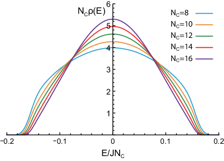
At fixed , as gets large, the many body DOS of Majorana or complex SYK globally approaches the Gaussian with a width . However, near the band edge , it shows the behaviour. So near the band edge, it locally behaves as a semi-circle. The expansion at a fixed at the temperatures can only resolve the local behaviour near the band edge, but not the global behaviour. In the double scaling limit and , but keep fixed, the action can be mapped to a 2d Liouville CFT in the kinetic space with the central charge which is solvable at all energy scales [86].The DOS was shown to be a Gaussian when , a semi-circle when , a more complicated form when ( see also the footnote [46] in Ref.[28] ). However, only in the triple scaling limit ( namely, the central charge ) and the low energy limit , at a fixed , it reduces to the 1d Schwarzian which is the low energy limit of the SYK model.
Appendix D The edge ( low and high energy) states versus the bulk ( intermediate energy ) states in and complex SYK
In this appendix, we aim to demonstrate the connections and differences between the edge and bulk states in the Fock space. They can be studied by studied by expansion or RG and RMT respectively. This appendix is heavily cited in Sec.VI.
1. Complex SYK model.

The complex SYK was written in Eq.15:
| (31) |
Instead of using the grand-canonical ensemble, we choose canonical one with a fixed fermion number . Then, the total Hilbert space can be decomposed into blocks as .
For , it is nothing but the single-particle sector with the dimension . Under the PH transformation , it is mapped to its particle-hole conjugate sector which is nothing but the single-hole sector. Surprisingly and interestingly, only the single-particle and the single-hole sector are chaotic in the GUE, all the other multi-particle sectors are integrable in the Possionian ( Fig.13 ).
As shown in Sec.III, , also maps to . For even, at the half-filling , so has a mirror symmetry for any realization of with respect to . This is indeed the case for in Fig.13. However, the exact mirror symmetry is absent away from the half-filling. But as argued below Eq.33, there is still an approximate mirror symmetry even away from the half-filling. Let us focus at the half-filling sector in the following.
As shown in Sec.V, the low energy spacing which stands for the low energy quasi-particle excitations, due to the exact mirror symmetry, the high energy spacing is also which stands for the high energy quasi-particle excitations. The bulk energy spacing is much smaller at a large . The KAM theorem is determined by the bulk energy spacing. All the bulk energy levels are described by the RMT in the Possion statistics. The bulk energy level statistics is quite in-sensitive to the edge energy levels. Namely, incorporating or throwing away these edge ( low or high energy ) levels will not affect the bulk Possion statistics.
2. Complex SYK model.

The complex SYK was also written in Eq.15:
| (32) |
As shown in Sec.III, , so in contrast to , does not have a mirror symmetry for any given random realization of . However, it still have an approximate mirror symmetry for any given realization of due to the following argument similar to Eq.18:
| (33) |
where . Note that we are still confining to the sector. Obviously, and satisfy the same distribution. At a large enough , it is self-averaging, so there is still an approximate mirror symmetry at any filling for a given random realization of .
This is indeed the case shown in Fig.14. As shown in Sec.VI, the low energy spacing , due to the approximate mirror symmetry, the high energy spacing is also . The bulk energy spacing is much smaller . The KAM theorem is determined by the bulk energy spacing. All the bulk energy levels are described by the RMT in the GOE. The bulk energy level statistics is quite in-sensitive to the edge energy levels. Namely, incorporating or throwing away these edge ( low or high energy ) levels will not affect the bulk GOE statistics.
References
- [1] A. I. Larkin and Y. N. Ovchinnikov, Quasi-classical method in the theory of superconductivity, Sov. Phys. JETP 28, 1200 (1969).
- [2] S. H. Shenker and D. Stanford, Black holes and the butterfly effect, J. High Energy Phys. 03 (2014) 067.
- [3] J. Maldacena, S. H. Shenker, and D. Stanford, A bound on chaos, J. High Energy Phys. 08 (2016) 106.
- [4] S. Sachdev and J. Ye, Gapless spin liuid ground state in a random quantum Heisenberg magnet, Phys. Rev. Lett. 70, 3339 (1993).
- [5] A. Georges, O. Parcollet, and S. Sachdev, Quantum fluctuations of a nearly critical Heisenberg spin glass, Phys. Rev. B 63, 134406 (2001).
- [6] A. Y. Kitaev, A simple model of quantum holography, talks at KITP, April 7, 2015 [http://online.kitp.ucsb.edu/online/entangled15/kitaev/], and May 27, 2015 [http://online.kitp.ucsb.edu/online/entangled15/kitaev2/].
- [7] S. Sachdev, Bekenstein-Hawking Entropy and Strange Metals, Phys. Rev. X 5, 041025 (2015).
- [8] J. Polchinski and V. Rosenhaus, The Spectrum in the Sachdev-Ye-Kitaev Model, J. High Energy Phys. 04 (2016) 001.
- [9] J. Maldacena and D. Stanford, Remarks on the Sachdev-Ye-Kitaev model, Phys. Rev. D 94, 106002 (2016).
- [10] W. Fu and S. Sachdev, Numerical study of fermion and boson models with infinite-range random interactions, Phys. Rev. B 94, 035135 (2016).
- [11] D. J. Gross and V. Rosenhaus, A Generalization of Sachdev-Ye-Kitaev, J. High Energy Phys. 02 (2017) 093.
- [12] D. Bagrets, A. Altland, and A. Kamenev, Sachdev-Ye-Kitaev model as Liouville quantum mechanics, Nucl. Phys. B 911, 191 (2016).
- [13] D. Bagrets, A. Altland, and A. Kamenev, Power-law out of time order correlation functions in the SYK model, Nucl. Phys. B 921, 727 (2017).
- [14] T. G. Mertens, G. J. Turiaci, H. L. Verlinde, Solving the Schwarzian via the Conformal Bootstrap, J. High Energy Phys. 08 (2017) 136.
- [15] D. Stanford, E. Witten, Fermionic Localization of the Schwarzian Theory, J. High Energy Phys. 10 (2017) 008.
- [16] J. Maldacena, D. Stanford, and Z. Yang, Conformal symmetry and its breaking in two dimensional Nearly Anti-de-Sitter space, Prog. Theor. Exp. Phys. 12 (2016) 12C104.
- [17] C. V. Johnson, Jackiw-Teitelboim supergravity, minimal strings, and matrix models, Phys. Rev. D 103, 046012 (2021).
- [18] C. V. Johnson, Explorations of nonperturbative Jackiw-Teitelboim gravity and supergravity, Phys. Rev. D 103, 046013 (2021).
- [19] A. Banerjee, A. Kundu, and R. R. Poojary, Rotating black holes in AdS spacetime, extremality, and chaos, Phys. Rev. D 102, 106013 (2020).
- [20] M. L. Mehta, Random Matrices and the Statistical Theory of Energy Levels, Chapter 16, (Academic Press, 1967).
- [21] C. E. Porter, Further remarks on energy level spacings, Nuclear Physics 40, 167 (1963),
- [22] P. B. Kahn and C. E. Porter, Statistical fluctuations of energy levels: The unitary ensemble, Nuclear Physics 48, 385 (1963).
- [23] Y.-Z. You, A. W. W. Ludwig, and C. Xu, Sachdev-Ye-Kitaev Model and Thermalization on the Boundary of Many-Body Localized Fermionic Symmetry Protected Topological States, Phys. Rev. B 95, 115150 (2017).
- [24] A. M. Garca-Garca and J. J.M. Verbaarschot, Spectral and thermodynamic properties of the Sachdev-Ye-Kitaev model, Phys. Rev. D 94, 126010 (2016).
- [25] J. S. Cotler, G. Gur-Ari, M. Hanada, J. Polchinski, P. Saad, S. H. Shenker, D. Stanford, A. Streicher, and M. Tezuka, Black Holes and Random Matrices, J. High Energy Phys. 05 (2017) 118 .
- [26] T. Li, J. Liu, Y. Xin, Y. Zhou, Supersymmetric SYK model and random matrix theory, J. High Energy Phys. 06 (2017) 111 .
- [27] T. Kanazawa, T. Wettig, Complete random matrix classification of SYK models with and 2 supersymmetry, J. High Energy Phys. 09 (2017) 050 .
- [28] F. Sun and J. Ye, Periodic Table of SYK and supersymmetric SYK, Phys. Rev. Lett. 124, 244101 (2020).
- [29] A. Altland and M. R. Zirnbauer, Nonstandard symmetry classes in mesoscopic normal-superconducting hybrid structures, Phys. Rev. B 55, 1142 (1997).
- [30] R. Gurau, The complete expansion of a SYK–like tensor model, Nucl. Phys. B 01 (2017) 015 .
- [31] E. Witten, An SYK-Like Model Without Disorder, J. Phys. A 52, 474002 (2019).
- [32] I. R. Klebanov, G. Tarnopolsky, Uncolored Random Tensors, Melon Diagrams, and the SYK Models, Phys. Rev. D 95, 046004 (2017).
- [33] T. Nishioka, Entanglement entropy: holography and renormalization group, Rev. Mod. Phys. 90, 035007 (2018).
- [34] X.-G. Wen, Colloquium: Zoo of quantum-topological phases of matter, Rev. Mod. Phys. 89, 041004 (2017).
- [35] X. Chen and A. W. W. Ludwig, Universal spectral correlations in the chaotic wave function and the development of quantum chaos, Phys. Rev. B 98, 064309 (2018).
- [36] V. J. Emery and S. Kivelson, Mapping of the two-channel Kondo problem to a resonant-level model, Phys. Rev. B 46, 10812 (1992). In fact, the non-zero impurity entropy at appears first in the two-channel Kondo model: is due to a decoupled Majorana fermion at the impurity side. It also leads to a non-Fermi liquid (or bad metal) behaviours (or absence of quasi-particles), which also happen here in SYK models.
- [37] A. W. W. Ludwig and I. Affleck, Exact conformal-field-theory results on the multi-channel Kondo effect: Asymptotic three-dimensional space- and time-dependent multi-point and many-particle Green’s functions, Nucl. Phys. B 428, 545 (1994).
- [38] J. M. Maldacena, A. W. W. Ludwig, Majorana Fermions, Exact Mapping between Quantum Impurity Fixed Points with four bulk Fermion species, and Solution of the “Unitarity Puzzle”, Nucl.Phys. B506, 565 (1997).
- [39] J. Ye, On Emery-Kivelson line and universality of Wilson ratio of spin anisotropic Kondo model, Phys. Rev. Lett. 77, 3224 (1996),
- [40] J. Ye, Abelian Bosonization approach to quantum impurity problems, Phys. Rev. Lett. 79, 1385 (1997).
- [41] A. Y. Kitaev, Anyons in an exactly solved model and beyond, Ann. Phys. 321, 2 (2006).
- [42] F. Sun, J. Ye, and W.-M. Liu, Quantum magnetism of spinor bosons in optical lattices with synthetic non-Abelian gauge fields, Phys. Rev. A 92, 043609 (2015).
- [43] For a concise review, see J. M. Deutsch, Eigenstate Thermalization Hypothesis, Rep. Prog. Phys. 81, 082001 (2018).
- [44] J. R. Garrison and T. Grover, Does a Single Eigenstate Encode the Full Hamiltonian?, Phys. Rev. X 8, 021026 (2018).
- [45] I. Kourkoulou, J. Maldacena, Pure states in the SYK model and nearly-AdS2 gravity, arXiv:1707.02325
- [46] Y. Y. Atas, E. Bogomolny, O. Giraud, and G. Roux, Distribution of the ratio of consecutive level spacings in random matrix ensembles. Phys. Rev. Lett. 110, 084101 (2013).
- [47] S. Ryu, A.P. Schnyder, A. Furusaki and A.W.W. Ludwig, Topological insulators and superconductors: Ten-fold way and dimensional hierarchy, New J. Phys. 12, 065010 (2010).
- [48] M. Z. Hasan and C. L. Kane, Colloquium: Topological insulators, Rev. Mod. Phys. 82, 3045 (2010).
- [49] X. L. Qi and S. C. Zhang, Topological insulators and superconductors, Rev. Mod. Phys. 83, 1057 (2011).
- [50] C.-K. Chiu, J.C.Y. Teo, A.P. Schnyder and S. Ryu, Classification of topological quantum matter with symmetries, Rev. Mod. Phys. 88, 035005 (2016).
- [51] In fact, equivalently, one can also define the PH symmetry operator to be . It is easy to show , , , where . The total number of fermions . It is not a conserved quantity, but the parity is in . Then which justifies as an anti-unitary PH transformation. Here does not provide any new information than , so is redundant. But they become important and in-dependent anti-unitary operators in the SUSY SYK [26, 27, 28]. For a unified and compact classification scheme on both SYK and SUSY SYK, see [28].
- [52] Here we choose even site to be real, odd site to be pure imaginary. Then as shown in our recent work [28], by choosing this way, when is odd, one must use the extended scheme (namely adding a Majorana fermion at to enlarge the Hilbert space twice, also introduce one more conserved quantity: the parity). However, if one choose the other way around, namely, even site to be pure imaginary, odd site to be real, then when is odd, one can use either the minimum scheme without adding a Majorana fermion at or the extended scheme.
- [53] It seems that so far, Ref.[23] and this work are the only two papers which have discussed the classifications and presented EDs in the odd case. But the two papers still use different anti-unitary operators to do the RMT classifications. For example, Ref.[23] constructed an anti-unitary Time-revresal operator in the many body Hilbert space, while we did not have such a kind of operator. It is still not known to the authors what are the relations between the two different sets of anti-unitary opartors. For a unified minimum classification scheme, see Ref.[28].
- [54] In fact, here we discuss a canonical ensemble instead of a grand canonical ensemble. So it has a fixed instead of a fixed .
- [55] In all the Figs.4-8, we get more noises on the side than those on the sides. This is because at a given , there are only random numbers on the side, while there are much more random numbers on the side. Of course, all -SYK are quite sparse in RMT sense. The side is just more sparse than the side.
- [56] L. Fidkowski and A. Kitaev, Topological phases of fermions in one dimension, Phys. Rev. B 83, 075103 (2011).
- [57] To do the ED, one [23, 10] puts the complex fermions on a chain with sites , then use the Jordan-Wigner transformation , (or equivalently , ) to map the spinless complex (or Majorana) fermion model to a quantum spin model, then do the ED in the equivalent quantum spin model. In this work, we did our ED in 3 independent ways (1) in the above spin basis after making the Jordan-Wigner transformation. (2) in the Hilbert space of complex fermions. As discussed in Sec.III-A, for odd , we add a Majorana fermion at . (3) using the Clifford algebra for both even and odd case. We achieved the same ED results in all the three ways.
- [58] To do the ED, following Ref.[10], one puts the hard core bosons on a chain with sites . The hard core boson case is simpler than its fermionic counterpart, because one do not need to attach a Jordan-Wigner string of , namely, , to map the hard core boson model to a quantum spin model.
- [59] It was known that the quantum ferromagnetic and anti-ferromagnetic Heisenberg model differs by only a sign. Despite they have dramatically different ground states and low energy excitations, using the same argument here, one can see they share the same ELS.
- [60] This choice is important when doing ED at a finite size . However, choosing the four site indices all different or not makes no difference in the expansion.
- [61] Z. Bi, C.-M. Jian, Y.-Z. You, K. A. Pawlak, C. Xu, Instability of the non-Fermi liquid state of the Sachdev-Ye-Kitaev Model, Phys. Rev. B 95, 205105 (2017).
- [62] A. Auerbach, Interacting electrons and quantum magnetism, (Springer Science & Business Media, 1994).
- [63] S. Sachdev, Quantum Phase transitions, (2nd edition, Cambridge University Press, 2011).
- [64] J. Ye and C.L. Zhang, Super-radiance, Photon condensation and its phase diffusion, Phys. Rev. A 84, 023840 (2011).
- [65] Yu Yi-Xiang, J. Ye and W.-M. Liu, Goldstone and Higgs modes of photons inside a cavity, Scientific Reports 3, 3476 (2013).
- [66] Yu Yi-Xiang, J. Ye, W.M. Liu and C.L. Zhang, Comments on “Controlling Discrete and Continuous Symmetries in Superradiant Phase Transitions with Circuit QED Systems”, arXiv:1506.06382.
- [67] Yu Yi-Xiang, J. Ye and C.L. Zhang, Parity oscillations and photon correlation functions in the Dicke model at a finite number of atoms or qubits, Phys. Rev. A 94, 023830 (2016).
- [68] Yu Yi-Xiang, J. Ye, W.-M. Liu and C. L. Zhang, Chaotic to integrable transition and a quantum analog of Kolmogorov-Arnold-Moser theorem in anisotrpoic Dicke model, un-published.
- [69] J. Ye, Two indices Sachdev-Ye-Kitaev model, arXiv:1809.0667, substantially revised version 2 to be put on arXiv soon.
- [70] R. Feng, G. Tian, D. Wei, Spectrum of SYK model, arXiv:1801.10073. Peking Math J. 2 (2019), No. 1, 41-70. Spectrum of SYK model II: Central limit theorem, arXiv:1806.05714; Spectrum of SYK model III: Large deviations and concentration of measures, arXiv:1806.04701. Random Matrices Theory Appl. 9 (2020), No. 2, 2050001 24pp. 60B20 (60F10)
- [71] F. Sun et. al., preprint in preparation.
- [72] A. Almheiri, Holographic Quantum Error Correction and the Projected Black Hole Interior, arXiv:1810.02055.
- [73] A. M. Garca-Garca, B. Loureiro, A. Romero-Bermdez, and M. Tezuka, Stability of chaos in a generalised Sachdev-Ye-Kitaev model, Phys. Rev. Lett. 120, 241603 (2018). Unfortunately, this paper confused CIT with the QPT. It even applied finite size scaling to the CIT. As demonstrated in Sec.V, CIT is dramatically different from the QPT, the finite size scaling applies to the latter only, NOT to the former.
- [74] T. Nosaka, D. Rosa, and J. Yoon, The Thouless time for mass-deformed SYK, J. High Energy Phys. 09 (2018) 041.
- [75] F. Sun, Yu Yi-Xiang, J. Ye and W.-M. Liu, Classifications of quantum chaos in colored Sachdev-Ye-Kitaev models, Phys. Rev. D 101, 026009 (2020).
- [76] E.P. Wigner, On the statistical distribution of the widths and spacings of nuclear resonance levels Proc. Camb. Phil. Soc., No. 47, 790 (1951).
- [77] F. Dyson, Statistical Theory of the Energy Levels of Complex Systems. I J. Math. Phys. (N.Y.) 3, 140 (1962).
- [78] K. Efetov, Supersymmetry in Disorder and Chaos, (Cambridge University Press, 1996 ).
- [79] J. Ye, Coulomb interaction at Superconductor to Mott-insulator transition, Phys. Rev. B 58, 9450 (1998).
- [80] J. Ye and S. Sachdev, The effects of Coulomb interaction on Quantum Hall critical points of systems in a periodic potential, Phys. Rev. Lett. 80, 5409 (1998).
- [81] J. Ye, The effects of weak disorders and Coulomb interaction on Quantum Hall critical points, Phys. Rev. B 60, 8290 (1999).
- [82] E.V. Shuryak and J.J.M Verbaarschot, Random matrix theory and spectral sum rules for the Dirac operator in QCD, Nucl. Phys. A 560 (1993) 306.
- [83] J.J.M. Verbaarschot, Spectrum of the QCD Dirac operator and chiral random matrix theory, Phys. Rev. Lett. 72, 2531 (1994).
- [84] Takuya Kanazawa, and Tilo Wettig, Stressed Cooper pairing in QCD at high isospin density: effective Lagrangian and random matrix theory, J. High Energy Phys. 1410 (2014) 55.
- [85] L. Herviou, J. H. Bardarson, and N. Regnault, Many-body localization in a fragmented Hilbert space, Phys. Rev. B 103 134207 (2021).
- [86] M. Berkooz, M. Isachenkov, V. Narovlansky, and G. Torrents, Towards a full solution of the large double-scaled SYK model, J. High Energy Phys. 03 (2019) 079.
- [87] Y. Gu, A. Kitaev, S. Sachdev, and G. Tarnopolsky, Notes on the complex Sachdev-Ye-Kitaev model, J. High Energy Phys. 02 (2020) 157.
- [88] In the Dicke model [65], at any finite , the gapless Goldstone mode at was lifted to a pseudo-Goldstone one with a finite gap where is the diffusion constant subject to an oscialltion due to the Berry phase. Then when adding a small CRW term smaller than this gap opened by the finite size effect, then the pseudo-Goldstone mode remains robust. This is more similar to the integrable side where the quasi-particle exists and has a gap , but dramatically different than the quantum chaostic side where the quasi-particle breaks down and has a much smaller gap and all the low energy levels are also stronglly repelled.
- [89] The edge states here mean the many body energy levels near the ground state, so they are ground state plus low energy excitations. The edge exponents in the RMT for the 7 classes with a mirror symmetry [28] mean the asympototic behvaiour of the lowest eigenvalue near the origin which, in the present case, is one of the bulk states. In some literatures, the former is called soft edge, the latter is hard edge.
- [90] There should be an exact proof on this Gaussian distribution in the many body DOS, see [71].
- [91] The two ways flow between the two CFT1 fixed points in Fig.9b1 and 9b2 violates the Zamoloddchikov’s c-theorem on RG flow between two CFT2 fixed points. See the conclusion section for more discussions.