Spectrum, Landau-Zener theory and driven-dissipative dynamics
of a staircase of photons
Abstract
We study the production of photons in a model of three bosonic atomic modes non-linearly coupled to a cavity mode. In absence of external driving and dissipation, the energy levels at different photon numbers assemble into the steps of an energy staircase which can be employed as guidance for preparing multi-photon states. We consider adiabatic photon production, driving the system through a sequence of Landau-Zener transitions in the presence of external coherent light pumping. We also analyse the non-equilibrium dynamics of the system resulting from the competition of the sudden switch of coherent photon pumping and cavity photon losses, and we find that the system approaches a plateau with a given number of photons, which becomes metastable upon increasing the rate of photon pumping. We discuss the sensitivity of the time scales for the onset of this metastable behaviour to system parameters and predict the value of photons attained, solving the driven-dissipative dynamics including three-body correlations between light and matter degrees of freedom.
pacs
05.30.Rt, 64.60.Ht , 75.10.JmI Introduction
The last ten years have witnessed swift progress in quantum optics platforms where light and matter are strongly coupled and can be employed to engineer a variety of quantum phenomena: examples range from Bose-Einstein condensates coupled to optical cavity photons, where the Dicke transition is engineered [1, 2], to the recent demonstration of supersolids [3] and phases with competing order parameters in a condensate trapped at the intersection of two optical cavities [4, 5, 6, 7]. Most of these models realise scenarios where matter and light collectively interact as in the case of superradiant phase transitions or in ’Dicke-Hubbard’ systems characterised by critical points separating a superfluid from a Mott insulating phase [8]. Strong light-matter coupling regimes have also enabled the preparation of highly squeezed states of atomic ensembles by quantum non-demolition measurements [9, 10], photon-mediated spin interactions [11, 12] in optical cavities, photon blockade effects [13, 14, 15, 16, 17] or non-classical light in cavity optomechanics platforms [18]. Recent experiments have extended photon-mediated interactions to optical-clock atoms [19], to spin-1 atoms [20, 21], and to multi-mode cavities [22], which enable further advances in quantum metrology [23] and quantum simulation.
The control and the preparation of multi-photon states is of paramount importance for a progress towards a many-body physics of coupled light and matter in these platforms. Single- and multi-photon preparation has a long history in cavity QED [24, 25, 26, 27, 28, 29, 30], including photon generation in high quality cavities [31], the control of single-photon states emitted by polaritons [32], as well as the conversion of collective atomic excitations into single photonic states within optical resonators [33], encompassing quantum homodyne tomography [34] and preparation of photon states in the driven dissipative dynamics of cavity arrays [35, 36].
In this work we consider a novel cavity-QED platform composed of collective atomic degrees of freedom strongly non-linearly coupled to a cavity photon: this system can be employed to engineer multi-photon states out of an empty cavity via adiabatic as well as with far-from-equilibrium driving protocols.
Specifically, we study an effective model of two bosonic atomic modes interacting with a photon; the model results from a two-photon resonant process occurring in a cavity hosting an ensemble of spin-1 atoms Rabi-coupled to the cavity mode. In equilibrium conditions, the eigenstates of this system compose a ‘staircase’ structure: each level, or ‘step’, is characterised by a different photon number which is a conserved quantity in undriven conditions. In the presence of weak coherent photonic pumping, an adiabatic variation in time of the energy levels of the atomic degrees of freedom allows for climbing the staircase, transiting across a sequence of level crossings, and thus preparing a desired number of photons out of an initially empty cavity.
Complementarily, we also consider the far-from-equilibrium dynamical preparation of photons in the system, suddenly switching the coherent photon pumping as well as including natural sources of dissipation, such as incoherent cavity-photon losses.
We highlight the formation of a metastable steady state in the late time driven-dissipative dynamics of photons, and discuss the dependence of its life-time on system parameters, solving the dynamics with the inclusion of three-body correlations between light and atomic degrees of freedom.
II The model
We consider an optical cavity supporting a photonic mode ( in Fig. 1) of frequency , Rabi coupled via the interaction coupling to the atoms. The three ground energy levels, e.g. Zeeman states in an atom of hyperfine spin ([20, 23, 21]), are denoted with , , , and the first two are detuned upwards and downwards, and with respect to the latter, which is assumed to have a macroscopic occupation, . A couple of external lasers of frequency can assist transitions from the two levels and to two auxiliary levels and respectively, with amplitudes . The lasers are far detuned from the transitions to the auxiliary levels by . Single-atom transitions assisted by the laser (or ) and by a cavity photon, transferring population from the states to (through levels and ) are off-resonant by an amount . However, transitions from the atomic state to , involving two atoms and assisted by a virtual photon emitted into the cavity and then rescattered, are resonant if the two detunings compensate each other, (a schematic of the energy levels and of the transitions is provided in Fig. 1). This resonant transition is pivotal for the realization of the photonic staircase at the core of this work, and the associated effective Hamiltonian reads
| (1) |
The last term embodies the photon-assisted resonance process changing simultaneously the population of the two atomic levels . In Eq. (1) we have reabsorbed the large occupation, , of the level in the coupling ; the mode can therefore be treated classically, while we assume that the occupation of the levels remains small. The frequency stands for the cavity mode frequency relative to the frequency of the lasers.
This derivation follows the lines of Ref. [37], considering three-level atoms Rabi coupled to a single mode optical cavity of frequency . Each atom has an internal structure consisting of the three states , , (ordered with decreasing energy), and the two states have a different Rabi coupling constant, , with the photonic cavity mode. With the energies of detunings, and , larger than all the other energy scales involved in the system, one can microscopically derive, via adiabatic elimination, the hamiltonian (1). We find that
| (2) |
where accounts for the quadratic Zeeman shift, and , assuming that the difference between (controlled by ) is smaller than their average.
Following this procedure, one finds that and are collective operators summing over all the single-particle excitations of the atoms, and they therefore have bosonic commutation relations.

III A staircase of photons
The hamiltonian (1) conserves the number of photons in the system, , allowing for diagonalization in sectors of the Hilbert space with fixed number of photons, . We describe, in each of these sectors, the lowest energy state using the variational ansatz state
| (3) |
where is the vacuum state simultaneously annihilated by . The unitary map transforms the operators and as
| (4) |
yielding the following expectation values
| (5) |
The latter expressions allow to compute the energy of the system, , on the ground-state variational ansatz, , and accordingly to find the value of the parameter, , yielding the minimum of the energy,
| (6) |
Using this equation we can, for instance, evaluate the population (and the coherences) of the level on the ground state
| (7) |
From Eq. (6), it follows that a real solution exists if
| (8) |
for parameters not satisfying this relation, the system exhibits an unstable behavior. The physical interpretation of Eq. (8) is that the strength of the photon-mediated interaction must be smaller than the quadratic Zeeman and AC Stark shifts for the system to be stable.
Indeed, a stability condition akin to (8) was already recognized in the context of coherent dissociation of a molecular condensate into a multiple-mode atomic one [38, 39, 40, 41]; if the molecular mode is highly occupied, one can linearize the Hamiltonian around the latter, and describe the process of dissociation with an Hamiltonian formally equivalent to (1) (in our system, the role of the highly occupied mode is taken by the level ). As a result of this, the coupling term does not conserve the number of particles created (annihilated) by () and for couplings violating (8), the eigenvalues of (1) becomes complex [38, 39, 40, 41] signalling an unstable character of the dynamics (cf. with Eq. (10) below).

The procedure resulting from Eq. (3), is equivalent to diagonalize the Hamiltonian (1) through the Bogolyubov rotation
| (9) |
with and ; the angle is, as usual, determined by requiring that off-diagonal terms proportional, for instance, to and its hermitian conjugate vanish (the result coincides with Eq. (8)). We can therefore write the diagonal form of (1) in a sector with fixed number of photons, ,
| (10) |
where the ground state energy of the system reads
| (11) |
The energy draws (as a function of ) a staircase in which each step is associated to a different value of . This is plotted in Fig. 2 together with few excited states energies (computed from Eq. (10)) plotted as dashed lines.

IV Landau-Zener theory
of the photons’ staircase
The staircase structure facilitates the preparation of a desired number of photons. In order to illustrate this aspect, we add to the hamiltonian, , a term, , accounting for coherent pumping of photons into the system at rate
| (12) |
Corrections to the spectrum are plotted in Fig. 3, and they can be evaluated exactly diagonalizing for few energy levels, using as basis the eigenstates of the unperturbed Hamiltonian (from now on we have dropped the dependence from in to lighten the notation). Our goal is to study Landau-Zener (LZ) transitions among ground state levels with different number of photons, as induced by a time-dependent control parameter, . It is possible to adiabatically climb the staircase without involving excited states in these transitions, if the drive occurs at an intermediate speed (see detailed discussion below).

We start writing the Hamiltonian in the basis , where it looks tri-diagonal since the perturbation couples states differing only by one photon; these are represented by off-diagonal terms in the following matrix representation of
| (13) |
The overlap is calculated following Ref. [43] as (see also Appendix)
| (14) |
In order to gain intuition for the perturbative corrections induced by a weak photon pumping on the photon staircase spectrum, we first consider a simple perturbative analysis in the parameters’ regime , . In this limit, the overlap reads , and the ground state energies, . Let us now consider an energy level , with photon number , crossing with a level with energy and ; at their intersection, occurring at , a straightforward application of degenerate perturbation theory in , yields an energy splitting
| (15) |
Beyond this simple analysis, an exact numerical evaluation of the eigenvalues of the energy matrix (13), as a function of , provides the energy level structure portrayed in the left panel of Fig. 3. A small pumping rate, , is sufficient to induce an effective energy level repulsion reshaping the staircase structure into a sequence of avoided crossings between ground states with different photon numbers. We remark that, although the coherent photon pumping does not commute with the unperturbed Hamiltonian (1), , its effect, for small , is negligible for values of away from the crossing points , and in these regions we can still effectively consider a good quantum number.
According to this structure, an adiabatic climbing of the staircase from a state with zero photons (blue line in the left panel of Fig. 3) to a state with a certain photonic population, can be designed as follows: We start from the ground state with zero photons and given initial at time , and we drive linearly in time the control parameter , with rate ; following the argument presented above, the drive can induce a transition to the ground state with one photon as approaches the crossing point located at (see the zoom of the crossing among and in the region : inset of left panel of Fig. 3).
For this LZ analysis, transitions involving excited states do not play a significant role. For instance, the transition from a ground state with photons into the first excited states of the next photonic manifold, such as a transition from to , or to , are assisted by matrix elements of the perturbation , which are smaller than the one connecting the two ground states. This is shown in the Appendix: Eqs. (24) and (25) display the matrix elements for the transition between the ground state and these two excited ones, and they should be compared with Eq. (14), reporting the overlap between ground states. The overlaps involving excited states are always smaller by a factor proportional to increasing powers of (a quantity always smaller than one) as higher excited states are considered. In particular, as grows large (i.e. increases, while the photonic manifolds of the staircase are explored) these overlaps are suppressed algrebraically in . We have numerically explored the specific case of the transition between the ground states of the first two photonic manifolds ( and ) in the right panel of Fig. 3 including the first excited state, and found that the weaker coupling to excited states discussed above, results into the possibility to perform adiabatic transitions among ground states. In Fig. 6 of the Appendix we show that the quantitative features of this adiabatic transition remain unaltered upon inclusion of the next excited state.
The right panel of Fig. 3 shows that a slow ramp would favour the transition to the first excited state of the manifold with one photon, but at intermediate ramp speeds, instead, the probability to transit into the ground state is the dominant one. As increases further, the subsequent transitions will basically occur between ground states of manifolds with different photon numbers (if the ramp is moderately slow), since, as discussed in the paragraph above, for the matrix elements of the operator controlling the transition, , become parametrically smaller than those connecting ground states and (see also the explicit expressions of these overlaps in the Appendix, Eqs. (A5) and (A6)). Therefore, a sequence of LZ-like transitions allows to climb the staircase and to achieve a target number of photons.
We observe that the jumps between the steps of the staircase characterised by different integer values of photons (see Fig. 4), and explored as is increased in time, recalls the current-voltage staircase profile observed in the phenomenon of Coulomb blockade [42].
Although the underlying mechanism is different, the two cases share the feature that every step of the staircase corresponds to a state with distinctly resolved physical properties: in our quantum optics set-up, for intervals of away from avoided crossings, each step of the staircase is associated to a fixed and quantised number of photons with negligible fluctuations.
Naturally, in the case of LZ photon preparation we expect that dissipation will classicalise the state of light at late times, but the staircase structure of the photonic response (see Fig 4) guarantees that, at intermediate times, the light degree of freedom will be found in a quantum state with a well defined number of photons and few fluctuations on the top of them, provided the time to implement the LZ ramp satisfies the condition . Furthermore, in order to have an adiabatic ramp and to remain in a weak photon pumping regime, we require also that . Since the coupling strength depends on the power in the optical drive fields and on detunings from atomic and cavity resonance, the ultimate limits are set by atomic and cavity parameters.
In particular, climbing the staircase requires large collective cooperativity , where is the single-atom cooperativity given the atomic excited-state linewidth . This requirement is derived from the scaling with of the atomic spontaneous emission rate and of Raman scattering into the cavity at rate . At an optimal detuning from Raman resonance, the coupling-to-dissipation ratio scales as . Thus, the requirement for climbing the staircase can be satisfied for large collective cooperativity . Collective cooperativities are routinely achieved with atomic ensembles in optical cavities, making the staircase accessible to current experiments.
V Driven-dissipative dynamics
We now consider the competition between coherent pumping and photon losses, occurring at rate and described by the jump operator (photon losses occurring during the intermediate processes contributing to the two-body resonance described in Fig. 1 are negligible in the far resonance regime as discussed in Ref. [44]). In particular, we will explore dynamics for times , where light becomes Poissonian as result of decoherence, at variance with the conditions discussed at the end of the previous Section (we will still assume large cooperativity and , though).
We consider a sudden switch of coherent pumping at times to counterbalance cavity losses. We prepare the system in the ground state of (1) with zero photons, , and we consider the time evolution ruled by the following set of equations of motion for the expectation values of the ’molecular’ degrees of freedom: atomic coherences, , and populations, ,
| (16) |
coupled to the dynamics of photons
| (17) |
where we have assumed the atomic and photonic degrees of freedom to be in a Gaussian state, and we have included terms describing three-body correlations between light and matter degrees of freedom, such as . The equation of motion for the the latter reads
| (18) |

During driven-dissipative dynamics the magnitude of three-body correlations between light and matter in Eqs. (16) and (17) remains small, with the consequence that the two sectors are almost dynamically decoupled. This allows the number of photons to relax towards a steady state value, , while the atomic excitations, , are still slowly growing as a consequence of the pumping. The steady-state number of photons generated is predicted by the formula
| (19) |
where is the asymptotic steady state value of . The time-scales separation in the dynamics of light and matter degrees of freedom is at the origin of the metastability of the plateau reached at long times by . In fact, a slow growth of (occurring while the photons’ steady state is already established), provokes a growth in as well, which acts as a source in Eq. (18) ruling the dynamics of . Therefore, the combination of bare photon pumping controlled by , and of effective pumping induced by three-body light-matter correlations, determines at later times an increase of , which can drive the system beyond the parameters’ region delimited by the condition in Eq. (8), where eigenenergies become imaginary (the associated critical value of the interaction strength in (8), is renormalised to a lower value after the inclusion of three-body light-matter correlations).
At the timescales for the departure from the metastable steady state, also the atomic and photonic correlations, evolving respectively under Eqs. (16) and (17), experience a quick, diverging growth. The characteristic time, , for the departure from the metastable photonic steady-state is proportional to : in Fig. 5 we portrait time-resolved profiles of at increasing pumping rates, , and we illustrate the metastability of the dynamics of as becomes sufficiently large. Fitting the breakdown time of the photonic plateau one finds that , which can be controlled both via the quadratic Zeeman and AC Stark shifts, and the occupation of the mode , as it can be realised by inspection of Eqs. (2) .
The inset of Fig. 5, displaying the average number of photons as function of , demonstrates instead that the quantization of typical of the staircase structure (still present when the photonic pumping is adiabatically switched and photons generated via slow LZ transitions) is lost when pumping and dissipation are suddenly turned on, since ground and excited states of the staircase are strongly mixed in this case.
Photon generation using ramps and LZ transitions are indeed more efficient than the sudden switching of photon pumping: In each one of the plateaux of Fig. 4 the photonic degree of freedom is in a state with fixed and quantised number of photons, , provided dissipation, , is weak enough to affect the dynamics of the system only at late times (see discussion at the end of Sec. IV). On the contrary, suddenly switching the photon pumping results in a transient dynamics with no quantised photon number (cf. Fig. 5), which asymptotes to a plateau where quantum features have been erased. Specifically, we have resolved the dynamics of our model combining a Gaussian ansatz for the atoms, as done in Eqs. (16), with a truncated ansatz for the density matrix of the light, , with and (see Appendix). Although in the plateaux shown in Fig. 5 the presence of the atomic degrees of freedom sizeably enhances the asymptotic expectation value of compared to the decoupled () case (and therefore the system is in a state where light and matter are hybridised), the light generated is classical, as we have checked by calculating the photonic variance, , from the density matrix ansatz, , found always very close to – a signature of the classical nature of the light produced in the cavity. This occurs for times , when the system has reached the steady state and at the same time the dissipation has washed out any quantum feature present at short times (see Appendix).
VI Perspectives
As a future direction, it would be interesting to study a many-body version of the problem analysed in this work, which can be realised, for instance, considering a one-dimensional lattice of several cavities (modelled as in Fig. 1), connected one to each other by next-neighbour photonic hoppings (in the spirit of an Hubbard model; see for similar ideas in quantum optics the review in [45]).
Studying the competition of this kinetic term with the
driving and dissipation discussed in this work, would pave the way to a quantum many body simulator for the preparation of multi-photon states, which would benefit of the tunability properties of the photons’ staircase as a leverage for experimental implementations. It would be, for instance, intriguing to look for driven-dissipative phase transitions in this many-body version of our system following the directions mentioned in the introduction.
VII Acknowledgments
We acknowledge discussions with F. Reiter. JM acknowledges support by the EU Horizon 2020 research and innovation program under Marie Sklodowska-Curie Grant Agreement No. 745608 (MC). YS and ED acknowledge support from Harvard-MIT CUA, NSF Grant No. DMR-1308435, AFOSR-MURI Quantum Phases of Matter (grant FA9550-14-1-0035), AFOSR-MURI Photonic Quantum Matter (award FA95501610323).
References
- [1] H. Keßler, J. Klinder, M. Wolke, and A. Hemmerich, Phys. Rev. Lett. 113, 070404 (2014).
- [2] K. Baumann, C. Guerlin, F. Brennecke, and T. Esslinger, Nature 464, 1301 (2010) .
- [3] J. Leonard, A. Morales, P. Zupancic, T. Esslinger, and T. Donner, Nature 543, 87-90 (2017a).
- [4] J. Leonard, A. Morales, P. Zupancic, T. Esslinger, and T. Donner, Science 358, 1415-1418 (2017b).
- [5] A. Morales, P. Zupancic, J. Leonard, T. Esslinger, and T. Donner, arXiv:1711.07988 (2017).
- [6] S. Gopalakrishnan, Y. E. Shchadilova, and E. A. Demler, Phys. Rev. A 96, 063828 (2017).
- [7] J. Lang, F. Piazza, and W. Zwerger, New Journal of Physics 19, 123027 (2017).
- [8] J. Klinder, H. Keßler, M. R. Bakhtiari, M. Thorwart, and A. Hemmerich, Phys. Rev. Lett. 115, 230403 (2015).
- [9] O. Hosten, N. Engelsen, K. R., and K. M., Nature, 529, 505 (2016) .
- [10] J. G. Bohnet, K. C. Cox, M. A. Norcia, J. M. Weiner, Z. Chen, and J. K. Thompson, Nat. Photon. 8, 731 (2014) .
- [11] I. D. Leroux, M. H. Schleier-Smith, and V. Vuletić, Phys. Rev. Lett. 104, 073602 (2010).
- [12] O. Hosten, R. Krishnakumar, N. Engelsen, and M. Kasevich, Science 352, 1552 (2016).
- [13] M. J. Hartmann, Fernando, G. S. L. Brandao, and M. B. Plenio, Nature Physics , 849 (2006).
- [14] C. Hamsen, K. N. Tolazzi, T. Wilk, and G. Rempe, Phys. Rev. Lett. 118, 133604 (2017).
- [15] V. Paulisch, M. Perarnau-Llobet, A. Gonzalez-Tudela, and J. I. Cirac, arXiv1805.00712 (2018).
- [16] A. Reinhard, T. Volz, M. Winger, A. Badolato, K. J. Hennessy, E. L. Hu, and A. Imamoglu, Nature Photonics 6, 93.
- [17] A. Imamoḡlu, H. Schmidt, G. Woods, and M. Deutsch, Phys. Rev. Lett. 79, 1467 (1997).
- [18] D. W. Brooks, T. Botter, S. Schreppler, T. P. Purdy, N. Brahms, and D. M. Stamper-Kurn, Nature 488, 476 (2012).
- [19] M. A. Norcia, R. J. Lewis-Swan, J. R. Cline, B. Zhu, A. M. Rey, and J. K. Thompson, Science 361, 259 (2018).
- [20] Z. Zhiqiang, C. H. Lee, R. Kumar, K. J. Arnold, S. J. Masson, A. S. Parkins, and M. D. Barrett, Optica 4, 424 (2017).
- [21] E. J. Davis, G. Bentsen, L. Homeier, T. Li, and M. H. Schleier-Smith, arXiv:1809.02114 (2018a).
- [22] V. D. Vaidya, Y. Guo, R. M. Kroeze, K. E. Ballantine, A. J. Kollár, J. Keeling, and B. L. Lev, Physical Review X 8, 011002 (2018).
- [23] S. J. Masson, M. D. Barrett, and S. Parkins, Phys. Rev. Lett. 119, 213601 (2017).
- [24] S. Brattke, B. T. H. Varcoe, and H. Walther, Phys. Rev. Lett. 86, 3534 (2001).
- [25] P. Bertet, S. Osnaghi, P. Milman, A. Auffeves, P. Maioli, M. Brune, J. M. Raimond, and S. Haroche, Phys. Rev. Lett. 88, 143601 (2002).
- [26] A. B. U’Ren, C. Silberhorn, K. Banaszek, and I. A. Walmsley, Phys. Rev. Lett. 93, 093601 (2004).
- [27] C. Sayrin and et al., Nature, 477, 73-77 (2011) .
- [28] M. Cooper, L. Wright, C. Söller, and B. Smith, Optics Express, 21, 5, 5309 (2013) .
- [29] D. I. Schuster, A. A. Houck, J. A. Schreier, A. Wallraff, J. M. Gambetta, A. Blais, L. Frunzio, J. Majer, B. Johnson, M. H. Devoret, S. M. Girvin, and R. J. Schoelkopf, Nature 445, 515 (2007).
- [30] M. Hafezi, P. Adhikari, and J. M. Taylor, Phys. Rev. B 92, 174305 (2015).
- [31] B. T. H. Varcoe, S. Brattke, M. Weidinger, and H. Walther, Nature, 403, 743-746 (2000) .
- [32] J. Stanojevic, V. Parigi, E. Bimbard, R. Tualle-Brouri, A. Ourjoumtsev, and P. Grangier, Phys. Rev. A 84, 053830 (2011).
- [33] J. Simon, H. Tanji, J. K. Thompson, and V. Vuletić, Phys. Rev. Lett. 98, 183601 (2007).
- [34] A. I. Lvovsky, H. Hansen, T. Aichele, O. Benson, J. Mlynek, and S. Schiller, Phys. Rev. Lett. 87, 050402 (2001).
- [35] A. Tomadin, V. Giovannetti, R. Fazio, D. Gerace, I. Carusotto, H. E. Türeci, and A. Imamoglu, Phys. Rev. A 81, 061801 (2010).
- [36] J. Lebreuilly, M. Wouters, and I. Carusotto, Comptes Rendus Physique 17, 836 (2016), polariton physics / Physique des polaritons.
- [37] J. Borregaard, E. J. Davis, G. S. Bentsen, M. H. Schleier-Smith, and A. S. Sorensen, New J. Phys. 19, 093021 (2017) .
- [38] A. Vardi, V. A. Yurovsky, and J. R. Anglin, Phys. Rev. A 64, 063611 (2001).
- [39] V. A. Yurovsky, A. Ben-Reuven, and P. S. Julienne, Phys. Rev. A 65, 043607 (2002).
- [40] J. R. Anglin, Phys. Rev. A 67, 051601 (2003).
- [41] M. A. Kayali and N. A. Sinitsyn, Phys. Rev. A 67, 045603 (2003).
- [42] Y. Alhassid, Rev. Mod. Phys. 72, 895 (2000).
- [43] A. M. Perelomov, Generalized Coherent States and Their Applications (Springer Verlag, 1986).
- [44] E. J. Davis, G. Bentsen, L. Homeier, T. Li, and M. H. Schleier-Smith, arXiv:1809.02111 (2018b).
- [45] A. Houck, H. E. Tureci, and J. Koch, Nature Physics 8, 292 (2012).
- [46] I. Vidanović, D. Cocks, and W. Hofstetter, Phys. Rev. A 89, 053614 (2014).
Appendix A Matrix elements for the Landau-Zener transition
In this section of the Appendix we detail the calculation of the matrix elements of the perturbation connecting ground and excited states of the staircase, involved in the study of the transitions in Fig. 3. The squeezed ground state (3) can be represented in the Fock basis of the occupation numbers of the modes, , as (see for instance Ref. [43])
| (20) |
where is the squeezing angle for a fixed number of photons, . We describe the excited states of the system using the quasiparticle creation operators and introduced in Eq. (9). We represent these operators inverting the Bogolyubov rotation (9):
| (21) |
Any excited state of the system can be represented as
| (22) |
with and .
In Eq. (12) we introduced a term accounting for coherent pumping of photons into the system at rate , . This term introduces mixing between the ground state in the sector with photons and excited states in the sector with photons. In order to account for this effect, we calculate the overlap of the excited states in the sector with photons with the ground state of the manifold with photons, .
First of all, we notice that the overlap between the excited states with quasiparticle excitations of only one type, and the ground state in the neighbouring sector, is equal to zero for any number of excitations ():
| (23) |
This is a consequence of the fact that the ground state (20) can be written as a superposition of states with the same number of excitations in the () sectors of the Fock space of the original degrees of freedom of the model.
The non-zero overlaps with excited states induced by the perturbation operator is between the state with quasiparticles in both () modes, . The first non-trivial overlap is . We calculate this overlap using the representation (20),
| (24) |
Analogously, we calculate the overlap
| (25) |
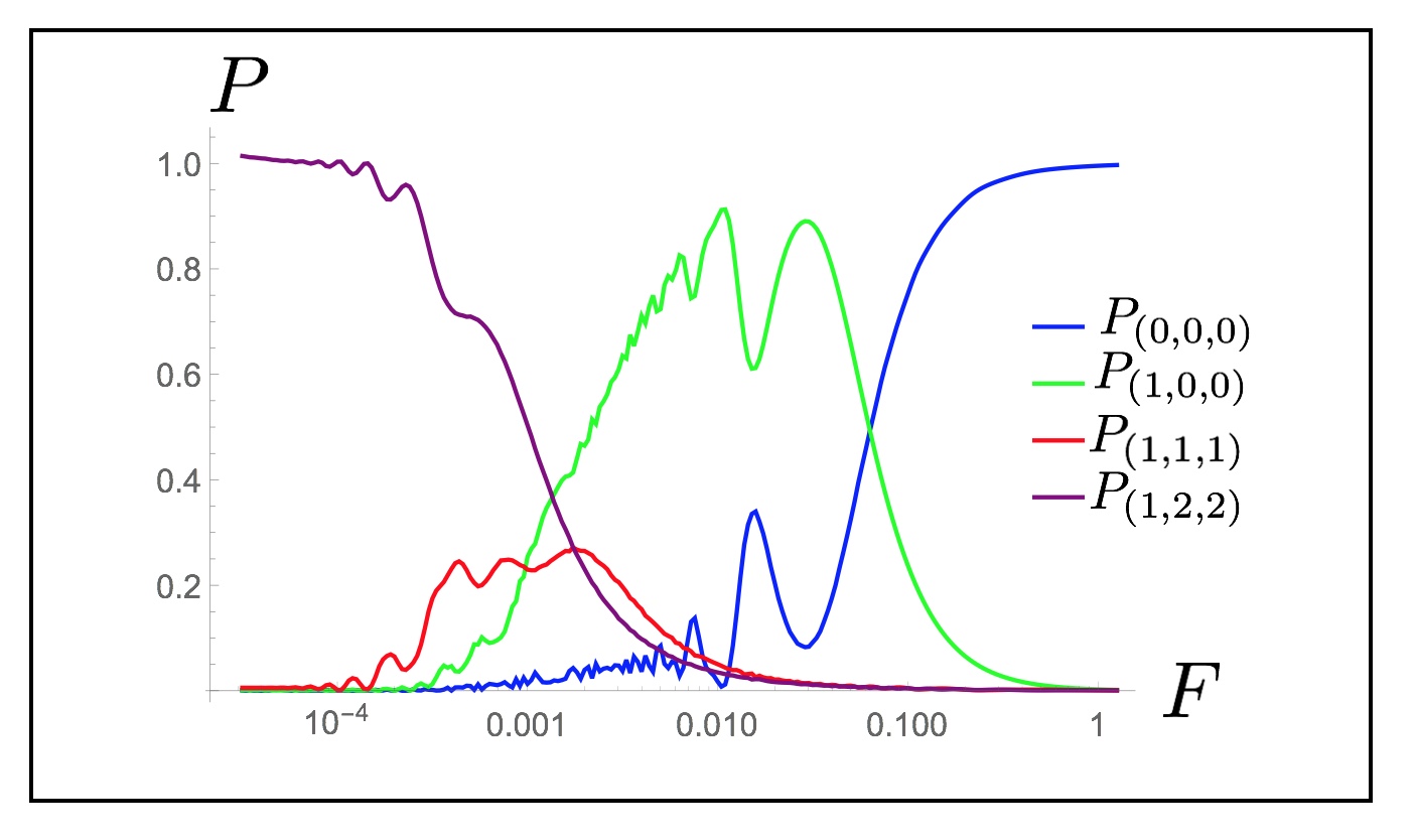
In these expressions one can recognise the overlap between the ground states of adjacent photonic manifolds, given by Eq. (14).
These overlaps allow to solve the LZ problem reported in Fig. 3b, and to check that adding the next excited state , the feature of an intermediate window of ramp speeds where the transition occurs only involving ground states, remains substantially unaffected. This is reported in Fig. 6 of this Appendix.
Appendix B Combined Gutzwiller and Gaussian ansätze for driven-dissipative dynamics
In this section of the Appendix we summarise the calculation of the photon variance , for which we resort to the following ansatz for the system density matrix:
| (26) |
where is a Gaussian ansatz density matrix for the atomic degrees of freedom, while for the photonic degree of freedom we write a density matrix in a bosonic Hilbert space truncated up to bosons:
| (27) |
with (we use in the following calculations). This is in spirit similar to the Gutzwiller ansatz employed in Ref. [46] for the dissipative dynamics of bosons. Inserting the ansatz (26) in the Lindblad equation
| (28) |
with incoherent photon losses at rate , we find that the equation of motions for the two-point functions of the atomic degrees of freedom follow Eqs. (16) (with three-body correlations set to zero), with the difference that now , while the equations (17) for the one and two-point functions of the photon are replaced by the linear system of equations of motion for the matrix elements of . As initial conditions, we consider . These equations appear cumbersome for large , but they can be readily derived. Here, for illustrative purposes, we write down the equations of motion for the population of the mode, , and for the first coherence, :
| (29) |
As a sanity check we benchmarked our predictions for in the exactly solvable case, .
The variance is then straightforwardly written in terms of the matrix elements of ,
| (30) |
An instance of the dynamics of is reported in Fig. 7, showing that at late times, . This circumstance is independent from the specific choice of parameters adopted.
