跳到论文正文
W Papers独立论文阅读器 arXiv:1809.07203 论文正文 计算阅读时间 · 0%
引用这篇论文根据当前论文元数据生成,正式投稿前建议核对。


License: CC BY-NC-SA 4.0
arXiv:1809.07203v2 [stat.AP] 09 Feb 2019

Parameter Estimation of Heavy-Tailed AR Model with Missing Data via Stochastic EM

Junyan Liu    Sandeep Kumar    and Daniel P. Palomar ††thanks: This work was supported by the Hong Kong RGC 16208917 research grant.††thanks: The authors are with the Hong Kong University of Science and Technology, Hong Kong (e-mail: jliubl@connect.ust.hk; eesandeep@ust.hk; palomar@ust.hk).
Abstract

The autoregressive (AR) model is a widely used model to understand time series data. Traditionally, the innovation noise of the AR is modeled as Gaussian. However, many time series applications, for example, financial time series data, are non-Gaussian, therefore, the AR model with more general heavy-tailed innovations is preferred. Another issue that frequently occurs in time series is missing values, due to system data record failure or unexpected data loss. Although there are numerous works about Gaussian AR time series with missing values, as far as we know, there does not exist any work addressing the issue of missing data for the heavy-tailed AR model. In this paper, we consider this issue for the first time, and propose an efficient framework for parameter estimation from incomplete heavy-tailed time series based on a stochastic approximation expectation maximization (SAEM) coupled with a Markov Chain Monte Carlo (MCMC) procedure. The proposed algorithm is computationally cheap and easy to implement. The convergence of the proposed algorithm to a stationary point of the observed data likelihood is rigorously proved. Extensive simulations and real datasets analyses demonstrate the efficacy of the proposed framework.

Index Terms: 
AR model, heavy-tail, missing values, SAEM, Markov chain Monte Carlo, convergence analysis

I Introduction

In the recent era of data deluge, many applications collect and process time series data for inference, learning, parameter estimation, and decision making. The autoregressive (AR) model is a commonly used model to analyze time series data, where observations taken closely in time are statistically dependent on others. In an AR time series, each sample is a linear combination of some previous observations with a stochastic innovation. An AR model of order pp, AR(pp), is defined as

yt=φ0+∑i=1pφi​yt−i+εt,y_{t}=\varphi_{0}+\sum_{i=1}^{p}\varphi_{i}y_{t-i}+\varepsilon_{t}, (1)

where yty_{t} is the tt-th observation, φ0\varphi_{0} is a constant, φi\varphi_{i}’s are autoregressive coefficients, and εt\varepsilon_{t} is the innovation associated with the tt-th observation. The AR model has been successfully used in many real-world applications such as DNA microarray data analysis [1], EEG signal modeling[2], financial time series analysis[3], and animal population study [4], to name but a few.

Traditionally, the innovation εt\varepsilon_{t} of the AR model is assumed to be Gaussian distributed, which, as a result of the linearity of the AR model, means that the observations are also Gaussian distributed. However, there are situations arising in applications of signal processing and financial markets where the time series are non-Gaussian and heavy-tailed, either due to intrinsic data generation mechanism or existence of outliers. Some examples are, stock returns [3, 5], brain fMRI [6, 7], and black-swan events in animal population [4]. For these cases, one may seek an AR model with innovations following a heavy-tailed distribution such as the Student’s tt-distribution. The Student’s tt-distribution is one of the most commonly used heavy-tailed distributions [8]. The authors of [9] and [10] have considered an AR model with innovations following a Student’s tt-distribution with a known number of degrees of freedom, whereas [11] and [12] investigated the case with an unknown number of degrees of freedom. The Student’s tt AR model performs well for heavy-tailed AR time series and can provide robust reliable estimates of the regressive coefficients when outliers occur.

Another issue that frequently occurs in practice is missing values during data observation or recording process. There are various reasons that can lead to missing values: values may not be measured, values may be measured but get lost, or values may be measured but are considered unusable [13]. Some real-world cases are: some stocks may suffer a lack of liquidity resulting in no transaction and hence no price recorded, observation devices like sensors may break down during measurement, and weather or other conditions disturb sample taking schemes. Therefore, investigation of AR time series with missing values is significant. Although there are numerous works considering Gaussian AR time series with missing values [14, 15, 16, 17], less attention has been paid to heavy-tailed AR time series with missing values, since parameter estimation in such a case is complicated due to the intractable problem formulation. The frameworks for parameter estimation for heavy-tailed AR time series in [9, 10, 11, 12] require complete data, and thereby, are not suited for scenarios with missing data. The objective of the current paper is to deal with this challenge and develop an efficient framework for parameter estimation from incomplete data under the heavy-tailed time series model via the expectation-maximization (EM) type algorithm.

The EM algorithm is a widely used iterative method to obtain the maximum likelihood (ML) estimates of parameters when there are missing values or unobserved latent variables. In each iteration, the EM algorithm maximizes the conditional expectation of the complete data likelihood to update the estimates. Many variants of the EM algorithm have been proposed to deal with specific challenges in different missing value problems. For example, to tackle the problem posed by the intractability of the conditional expectation of the complete data log-likelihood, a stochastic variant of the EM algorithm, which approximates the expectation by drawing samples of the latent variables from the conditional distribution, has been proposed in [18, 19]. The stochastic EM has also been quite popular to curb the curse of dimensionality [20, 14], since its computation complexity is lower than the EM algorithm. The expectation conditional maximization (ECM) algorithm has been suggested to deal with the unavailability of the closed-form maximizer of the expected complete data log-likelihood [21]. The regularized EM algorithm has been used to enforce certain structures in parameter estimates like sparsity, low-rank, and network structure [22].

In this paper, we develop a provably convergent low cost algorithmic framework for parameter estimation of the AR time series model with heavy-tailed innovations from incomplete time series. As far as we know, there does not exist any convergent algorithmic framework for such problem. Following [9, 10, 11], here we consider the AR model with the Student’s tt distributed innovations. We formulate an ML estimation problem and develop an efficient algorithm to obtain the ML estimates of the parameters based on the stochastic EM framework. To tackle the complexity of the conditional distribution of latent variables, we propose a Gibbs sampling scheme to generate samples. Instead of directly sampling from the complicated conditional distribution, the proposed algorithm just need to sample from Gaussian distributions and gamma distributions alternatively. The convergence of the proposed algorithm to a stationary point is established. Simulations on real data and synthetic data show that the proposed framework can provide accurate estimation of parameters for incomplete time series, and is also robust against possible outliers. Although here we only focus on the Student’s tt distributed innovation, the idea of the proposed approach and the algorithm can also be extended to the AR model with other heavy-tailed distributions.

This paper is organized as follows. The problem formulation is provided in Section II. The review of the EM and its stochastic variants is presented in Section III. The proposed algorithm is derived in Section IV. The convergence analysis is carried out in Section V. Finally, Simulation results for the proposed algorithm applied to both real and synthetic data are provided in Section VI, and Section VII concludes the paper.

II Problem Formulation

For simplicity of notations, we first introduce the AR(1) model. Suppose a univariate time series y1y_{1}, y2y_{2},…\ldots, yTy_{T} follows an AR(11) model

yt=φ0+φ1​yt−1+εt,y_{t}=\varphi_{0}+\varphi_{1}y_{t-1}+\varepsilon_{t}, (2)

where the innovations εt\varepsilon_{t}’s follow a zero-mean heavy-tailed Student’s tt-distribution εt​∼i.i.d.​t​(0,σ2,ν)\varepsilon_{t}\overset{i.i.d.}{\sim}t\left(0,\sigma^{2},\nu\right). The Student’s tt-distribution is more heavy-tailed as the number of degrees of freedom ν\nu decreases. Note that the Gaussian distribution is a special case of the Student’s tt-distribution with ν=+∞.\nu=+\text{$\infty$}.

Given all the parameters φ0\varphi_{0}, φ1\varphi_{1}, σ2\sigma^{2} and ν\nu, the distribution of yty_{t} conditional on all the preceding data ℱt−1\mathcal{F}_{t-1}, which consists of y1y_{1},y2y_{2}, …\ldots,yt−1y_{t-1}, only depends on the previous sample yt−1y_{t-1}:

p⁡(yt|φ0,φ1,σ2,ν,ℱt−1)\displaystyle p\left(y_{t}|\varphi_{0},\varphi_{1},\sigma^{2},\nu,\mathcal{F}_{t-1}\right) (3)
=p⁡(yt|φ0,φ1,σ2,ν,yt−1)\displaystyle=p\left(y_{t}|\varphi_{0},\varphi_{1},\sigma^{2},\nu,y_{t-1}\right)
=ft​(yt,φ0+φ1​yt−1,σ2,ν)\displaystyle=f_{t}\left(y_{t};\varphi_{0}+\varphi_{1}y_{t-1},\sigma^{2},\nu\right)
=Γ⁡(ν+12)ν​π​σ​Γ​(ν2)​(1+(yt−φ0−φ1​yt−1)2ν​σ2)−ν+12,\displaystyle=\frac{\Gamma\left(\frac{\nu+1}{2}\right)}{\sqrt{\nu\pi}\sigma\Gamma\left(\frac{\nu}{2}\right)}\left(1+\frac{\left(y_{t}-\varphi_{0}-\varphi_{1}y_{t-1}\right)^{2}}{\nu\sigma^{2}}\right)^{-\frac{\nu+1}{2}},

where ft​(⋅)f_{t}\left(\cdot\right) denotes the probability density function (pdf) of a Student’s tt-distribution.

In practice, a certain sample yty_{t} may be missing due to various reasons, and it is denoted by yt=𝖭𝖠y_{t}=\mathsf{NA} (not available). Here we assume that the missing-data mechanism is ignorable, i.e., the missing does not depend on the value [13]. Suppose we have an observation of this time series with DD missing blocks as follows:

y1,…,yt1,𝖭𝖠,…,𝖭𝖠,yt1+n1+1,…​ytd,𝖭𝖠,…,𝖭𝖠,\displaystyle y_{1},\ldots,y_{t_{1}},\mathsf{NA},\ldots,\mathsf{NA},y_{t_{1}+n_{1}+1},\ldots y_{t_{d}},\mathsf{NA},\ldots,\mathsf{NA},
ytd+nd+1,…,ytD,𝖭𝖠,…,𝖭𝖠,ytD+nD+1,…,yT,\displaystyle y_{t_{d}+n_{d}+1},\ldots,y_{t_{D}},\mathsf{NA},\ldots,\mathsf{NA},y_{t_{D}+n_{D}+1},\ldots,y_{T},

where, in the dd-th missing block, there are ndn_{d} missing samples ytd+1y_{t_{d}+1},…\ldots,ytd+ndy_{t_{d}+n_{d}}, which are surrounded from the left and the right by the two observed data ytdy_{t_{d}} and ytd+nd+1y_{t_{d}+n_{d}+1}. We set for convenience t0=0t_{0}=0 and n0=0n_{0}=0. Let us denote the set of the indexes of the observed values by C𝗈C_{\mathsf{o}}, and the set of the indexes of the missing values by C𝗆C_{\mathsf{m}}. Also denote 𝐲=(yt, 1≤t≤T)\mathbf{y}=\left(y_{t},\thinspace 1\leq t\leq T\right), 𝐲𝗈=(yt,t∈C𝗈)\mathbf{y}_{\mathsf{o}}=\left(y_{t},\thinspace t\in C_{\mathsf{\mathsf{o}}}\right), and 𝐲𝗆=(yt,t∈C𝗆)\mathbf{y}_{\mathsf{m}}=\left(y_{t},\thinspace t\in C_{\mathsf{m}}\right) .

Let us assume 𝜽=(φ0,φ1,σ2,ν)∈Θ\boldsymbol{\theta}=\left(\varphi_{0},\varphi_{1},\sigma^{2},\nu\right)\in\Theta with Θ={𝜽|σ2>0,ν>0}.\Theta=\left\{\boldsymbol{\theta}|\sigma^{2}>0,\thinspace\nu>0\right\}. Ignoring the marginal distribution of y1y_{1}, the log-likelihood of the observed data is

l⁡(𝜽,𝐲𝗈)=\displaystyle l\left(\boldsymbol{\theta};\mathbf{y}_{\mathsf{o}}\right)= log⁡(∫p⁡(𝐲,𝜽)​𝖽​𝐲𝗆)\displaystyle\log\left(\int p\left(\mathbf{y};\boldsymbol{\theta}\right)\mathsf{d}\mathbf{y}_{\mathsf{m}}\right)
=\displaystyle= log⁡(∫∏t=2Tp⁡(yt|𝜽,ℱt−1)​𝖽​𝐲𝗆)\displaystyle\log\left(\int\prod_{t=2}^{T}p\left(y_{t}|\boldsymbol{\theta},\mathcal{F}_{t-1}\right)\mathsf{d}\mathbf{y}_{\mathsf{m}}\right) (4)
=\displaystyle= log⁡(∫∏t=2Tft​(yt,φ0+φ1​yt−1,σ2,ν)​𝖽​𝐲𝗆).\displaystyle\log\left(\int\prod_{t=2}^{T}f_{t}\left(y_{t};\varphi_{0}+\varphi_{1}y_{t-1},\sigma^{2},\nu\right)\mathsf{d}\mathbf{y}_{\mathsf{m}}\right).

Then the maximum likelihood (ML) estimation problem for 𝜽\boldsymbol{\theta} can be formulated as

𝗆𝖺𝗑𝗂𝗆𝗂𝗓𝖾𝜽∈Θ\displaystyle\mathsf{\underset{\boldsymbol{\theta}\in\Theta}{maximize}} l⁡(𝜽,𝐲𝗈).\displaystyle l\left(\boldsymbol{\theta};\mathbf{y}_{\mathsf{o}}\right). (5)

The integral in (4) has no closed-form expression, thus, the objective function is very complicated, and we cannot solve the optimization problem directly. In order to deal with this, we resort to the EM framework, which circumvents such difficulty by optimizing a sequence of simpler approximations of the original objective function instead.

III EM and Its Stochastic Variants

The EM algorithm is a general iterative algorithm to solve ML estimation problems with missing data or latent data. More specifically, given the observed data 𝐗\mathbf{X} generated from a statistical model with unknown parameter 𝜽\boldsymbol{\theta}, the ML estimator of the parameter 𝜽\boldsymbol{\theta} is defined as the maximizer of the likelihood of the observed data

l⁡(𝐗,𝜽)=log⁡p⁡(𝐗|𝜽).l\left(\mathbf{X};\boldsymbol{\theta}\right)=\log p(\mathbf{X}|\boldsymbol{\theta}). (6)

In practice, it often occurs that l⁡(𝐗,𝜽)l\left(\mathbf{X};\boldsymbol{\theta}\right) does not have manageable expression due to the missing data or latent data 𝐙\mathbf{Z}, while the likelihood of complete data p⁡(𝐗,𝐙|𝜽)p(\mathbf{X},\mathbf{Z}|\boldsymbol{\theta}) has a manageable expression. This is when the EM algorithm can help. The EM algorithm seeks to find the ML estimates by iteratively applying these two steps [23]:

(E)

Expectation: calculate the expected log-likelihood of the complete data set (𝐗,𝐙)\left(\mathbf{X},\mathbf{Z}\right) with respect to the current conditional distribution of 𝐙\mathbf{Z} given 𝐗\mathbf{X} and the current estimate of the parameter 𝜽(k)\mathbf{\boldsymbol{\theta}}^{\left(k\right)}:

Q⁡(𝜽|𝜽(k))=∫log⁡p⁡(𝐗,𝐙|𝜽)​p​(𝐙|𝐗,𝜽(k))​𝑑𝐙,Q\left(\boldsymbol{\theta}|\boldsymbol{\theta}^{\left(k\right)}\right)=\int\log p\left(\mathbf{X},\thinspace\mathbf{Z}|\boldsymbol{\theta}\right)p\left(\mathbf{Z}|\mathbf{X},\boldsymbol{\theta}^{\left(k\right)}\right)\mathsf{d}\mathbf{Z}, (7)

where kk is the iteration number.

(M)

Maximization: find the new estimate

𝜽(k+1)=arg⁡max𝜽​Q​(𝜽|𝜽(k)).\mathbf{\boldsymbol{\theta}}^{\left(k+1\right)}=\underset{\boldsymbol{\theta}}{\arg\max\thinspace}Q\left(\boldsymbol{\theta}|\mathbf{\boldsymbol{\theta}}^{\left(k\right)}\right). (8)

The sequence {l⁡(𝐗,𝜽(k))}\left\{l\left(\mathbf{X};\boldsymbol{\theta}^{\left(k\right)}\right)\right\} generated by the EM algorithm is non-decreasing, and the limit points of the sequence {𝜽(k)}\left\{\mathbf{\boldsymbol{\theta}}^{\left(k\right)}\right\} are proven to be the stationary points of the observed data log-likelihood under mild regularity conditions [24]. In fact, the EM algorithm is a particular choice of the more general majorization-minimization algorithm [25].

However, in some applications of the EM algorithm, the expectation in the E step cannot be obtained in closed-form. To deal with this, Wei and Tanner proposed the Monte Carlo EM (MCEM) algorithm, in which the expectation is computed by a Monte Carlo approximation based on a large number of independent simulations of the missing data [26]. The MCEM algorithm is computationally very intensive.

In order to reduce the amount of simulations required by the MCEM algorithm, the stochastic approximation EM (SAEM) algorithm replaces the E step of the EM algorithm by a stochastic approximation procedure, which approximates the expectation by combining new simulations with the previous ones [18]. At iteration kk, the SAEM proceeds as follows:

(E-S1)

Simulation: generate LL realizations 𝐙(k,l)\mathbf{Z}^{\left(k,l\right)} (l=1,2​…,L)\left(l=1,2\ldots,L\right) from the conditional distribution p⁡(𝐙|𝐗,𝜽(k))p\left(\mathbf{Z}|\mathbf{X},\boldsymbol{\theta}^{\left(k\right)}\right)

(E-A)

Stochastic approximation: update Q^​(𝜽|𝜽(k))\hat{Q}\left(\boldsymbol{\theta}|\boldsymbol{\theta}^{\left(k\right)}\right) according to

Q^​(𝜽|𝜽(k))\displaystyle\hat{Q}\left(\boldsymbol{\theta}|\boldsymbol{\theta}^{\left(k\right)}\right) (9)
=Q^​(𝜽|𝜽(k−1))+γ(k)​(1L​∑l=1Llog⁡p⁡(𝐗,𝐙(k,l)|𝜽)CLOSE\displaystyle=\hat{Q}\left(\boldsymbol{\theta}|\boldsymbol{\theta}^{\left(k-1\right)}\right)+\gamma^{\left(k\right)}\biggl(\frac{1}{L}\sum_{l=1}^{L}\log p\left(\mathbf{X},\thinspace\mathbf{Z}^{\left(k,l\right)}|\boldsymbol{\theta}\right)
OPEN−Q^​(𝜽|𝜽(k−1))),\displaystyle-\hat{Q}\left(\boldsymbol{\theta}|\boldsymbol{\theta}^{\left(k-1\right)}\right)\biggr),

where {γ(k)}\left\{\gamma^{\left(k\right)}\right\} is a decreasing sequence of positive step sizes.

(M)

Maximization: find the new estimate

𝜽(k+1)=arg⁡max𝜽​Q^​(𝜽|𝜽(k)).\mathbf{\boldsymbol{\theta}}^{\left(k+1\right)}=\underset{\boldsymbol{\theta}}{\arg\max\thinspace}\hat{Q}\left(\boldsymbol{\theta}|\boldsymbol{\theta}^{\left(k\right)}\right). (10)

The SAEM requires a smaller amount of samples per iteration due to the recycling of the previous simulations. A small value of LL is enough to ensure satisfying results [27].

When the conditional distribution is very complicated, and the simulation step (E-S1) of the SAEM cannot be directly performed, Kuhn and Lavielle proposed to combine the SAEM algorithm with a Markov Chain Monte Carlo (MCMC) procedure, which yields the SAEM-MCMC algorithm [19]. Assume the conditional distribution p⁡(𝐙|𝐗,𝜽)p\left(\mathbf{Z}|\mathbf{X},\boldsymbol{\theta}\right) is the unique stationary distribution of the transition probability density function Π𝜽\Pi_{\boldsymbol{\theta}}, the simulation step of the SAEM is replaced with

(E-S2)

Simulation: draw realizations 𝐙(k,l)\mathbf{Z}^{\left(k,l\right)} (l=1,2​…,L)\left(l=1,2\ldots,L\right) based on the transition probability density function Π𝜽(k)​(𝐙(k−1,l),⋅)\Pi_{\boldsymbol{\theta}^{\left(k\right)}}\left(\mathbf{Z}^{\left(k-1,l\right)},\cdot\right).

For each ll, the sequence {𝐙(k,l)}k≥0\left\{\mathbf{Z}^{\left(k,l\right)}\right\}_{k\geq 0} is a Markov chain with the transition probability density function {Π𝜽(k)}.\left\{\Pi_{\boldsymbol{\theta}^{\left(k\right)}}\right\}. The Markov Chain generation mechanism needs to be well designed so that the sampling is efficient and the computational cost is not too high.

IV SAEM-MCMC for Student’s tt AR Model

For the ML problem (5), if we only regard 𝐲𝗆\mathbf{y}_{\mathsf{m}} as missing data and apply the EM type algorithm, the resulting conditional distribution of the missing data is still complicated, and it is difficult to maximize the expectation or the approximated expectation of the complete data log-likelihood. Interestingly, the Student’s tt-distribution can be regarded as a Gaussian mixture [2]. Since εt∼t⁡(0,σ2,ν)\varepsilon_{t}\sim t\left(0,\sigma^{2},\nu\right), we can present it as a Gaussian mixture

εt|σ2,τt∼𝒩⁡(0,σ2τt),\varepsilon_{t}|\sigma^{2},\tau_{t}\thicksim\mathcal{N}\left(0,\frac{\sigma^{2}}{\tau_{t}}\right), (11)
τt∼G​a​m​m​a​(ν/2,ν/2),\tau_{t}\thicksim Gamma\left(\nu/2,\thinspace\nu/2\right), (12)

where τt\tau_{t} is the mixture weight. Denote 𝝉={τt, 1<t≤T}\boldsymbol{\tau}=\left\{\tau_{t},\thinspace 1<t\leq T\right\}. We can use the EM type algorithm to solve the above optimization problem by regarding both 𝐲𝗆\mathbf{y}_{\mathsf{m}} and 𝝉\boldsymbol{\tau} as latent data, and 𝐲𝗈\mathbf{y}_{\mathsf{o}} as observed data.

The resulting complete data likelihood is

L⁡(𝜽,𝐲,𝝉)\displaystyle L\left(\boldsymbol{\theta};\mathbf{y},\boldsymbol{\tau}\right) (13)
=p⁡(𝐲,𝝉,𝜽)\displaystyle=p\left(\mathbf{y},\boldsymbol{\tau};\boldsymbol{\theta}\right)
=∏t=2T{fN​(yt,φ0+φ1​yt−1,σ2τt)​fg​(τt,ν2,ν2)}\displaystyle=\prod_{t=2}^{T}\left\{f_{N}\left(y_{t};\varphi_{0}+\varphi_{1}y_{t-1},\frac{\sigma^{2}}{\tau_{t}}\right)f_{g}\left(\tau_{t};\frac{\nu}{2},\frac{\nu}{2}\right)\right\}
=∏t=2T{12​π​σ2/τtexp(−12​σ2/τt(yt−φ0−φ1yt−1)2)\displaystyle=\prod_{t=2}^{T}\Biggl\{\frac{1}{\sqrt{2\pi\sigma^{2}/\tau_{t}}}\exp\left(-\frac{1}{2\sigma^{2}/\tau_{t}}\left(y_{t}-\varphi_{0}-\varphi_{1}y_{t-1}\right)^{2}\right)
(ν2)ν2Γ⁡(ν2)τtν2−1exp(−ν2τt)}\displaystyle\frac{\left(\frac{\nu}{2}\right)^{\frac{\nu}{2}}}{\Gamma\left(\frac{\nu}{2}\right)}\tau_{t}^{\frac{\nu}{2}-1}\exp\left(-\frac{\nu}{2}\tau_{t}\right)\Biggr\}
=∏t=2T(ν2)ν2​τtν−12Γ⁡(ν2)​2​π​σ2​exp⁡(−τt2​σ2​(yt−φ0−φ1​yt−1)2−ν2​τt),\displaystyle=\prod_{t=2}^{T}\frac{\left(\frac{\nu}{2}\right)^{\frac{\nu}{2}}\tau_{t}^{\frac{\nu-1}{2}}}{\Gamma\left(\frac{\nu}{2}\right)\sqrt{2\pi\sigma^{2}}}\exp\left(-\frac{\tau_{t}}{2\sigma^{2}}\left(y_{t}-\varphi_{0}-\varphi_{1}y_{t-1}\right)^{2}-\frac{\nu}{2}\tau_{t}\right),

where fN​(⋅)f_{N}\left(\cdot\right) and fg​(⋅)f_{g}\left(\cdot\right) denote the pdf’s of the Normal (Gaussian) and gamma distributions, respectively. Through some simple derivation, it is observed that the likelihood of complete data belongs to the curved exponential family [29], i.e., the pdf can be written as

L⁡(𝜽,𝐲,𝝉)=h⁡(𝐲,𝝉)​exp⁡(−ψ⁡(𝜽)+⟨𝐬⁡(𝐲𝗈,𝐲𝗆,𝝉),ϕ⁡(𝜽)⟩),L\left(\boldsymbol{\theta};\mathbf{y},\boldsymbol{\tau}\right)=h\left(\mathbf{y},\boldsymbol{\tau}\right)\exp\left(-\psi\left(\boldsymbol{\theta}\right)+\left\langle\mathbf{s}\left(\mathbf{y}_{\mathsf{o}},\mathbf{y}_{\mathsf{m}},\boldsymbol{\tau}\right),\boldsymbol{\phi}\left(\boldsymbol{\theta}\right)\right\rangle\right), (14)

where ⟨⋅,⋅⟩\left\langle\cdot,\cdot\right\rangle is the inner product,

h⁡(𝐲,𝝉)=∏t=2Tτt−12,h\left(\mathbf{y},\boldsymbol{\tau}\right)=\prod_{t=2}^{T}\tau_{t}^{-\frac{1}{2}}, (15)
ψ⁡(𝜽)=\displaystyle\psi\left(\boldsymbol{\theta}\right)= −(T−1){ν2log(ν2)−log(Γ(ν2))\displaystyle-\left(T-1\right)\Biggl\{\frac{\nu}{2}\log\left(\frac{\nu}{2}\right)-\log\left(\Gamma\left(\frac{\nu}{2}\right)\right) (16)
−12log(σ2)−12log(2π)},\displaystyle-\frac{1}{2}\log\left(\sigma^{2}\right)-\frac{1}{2}\log\left(2\pi\right)\Biggr\},
ϕ⁡(𝜽)=[ν2,−12​σ2,−φ022​σ2,−φ122​σ2,φ0σ2,φ1σ2,−φ0​φ1σ2],\boldsymbol{\phi}\left(\boldsymbol{\theta}\right)=\left[\frac{\nu}{2},\thinspace-\frac{1}{2\sigma^{2}},\thinspace-\frac{\varphi_{0}^{2}}{2\sigma^{2}},\thinspace-\frac{\varphi_{1}^{2}}{2\sigma^{2}},\thinspace\frac{\varphi_{0}}{\sigma^{2}},\thinspace\frac{\varphi_{1}}{\sigma^{2}},\thinspace-\frac{\varphi_{0}\varphi_{1}}{\sigma^{2}}\right], (17)

and the minimal sufficient statistics

𝐬⁡(𝐲𝗈,𝐲𝗆,𝝉)=\displaystyle\mathbf{s}\left(\mathbf{y}_{\mathsf{o}},\mathbf{y}_{\mathsf{m}},\boldsymbol{\tau}\right)= [∑t=2T(log(τt)−τt),∑t=2Tτtyt2,∑t=2Tτt,∑t=2Tτtyt−12,\displaystyle\Biggl[\sum_{t=2}^{T}\left(\log\left(\tau_{t}\right)-\tau_{t}\right),\sum_{t=2}^{T}\tau_{t}y_{t}^{2},\sum_{t=2}^{T}\tau_{t},\sum_{t=2}^{T}\tau_{t}y_{t-1}^{2},
∑t=2Tτtyt,∑t=2Tτtytyt−1,∑t=2Tτtyt−1].\displaystyle\sum_{t=2}^{T}\tau_{t}y_{t},\sum_{t=2}^{T}\tau_{t}y_{t}y_{t-1},\sum_{t=2}^{T}\tau_{t}y_{t-1}\Biggr]. (18)

Then the expectation of the complete data log-likelihood can be expressed as

Q⁡(𝜽|𝜽(k))\displaystyle Q\left(\boldsymbol{\theta}|\boldsymbol{\theta}^{\left(k\right)}\right)
=∬log(L(𝜽;𝐲,𝝉))p(𝐲𝗆,𝝉|𝐲𝗈;𝜽(k))𝖽𝐲𝗆𝖽𝝉\displaystyle=\iint\log\left(L\left(\boldsymbol{\theta};\mathbf{y},\boldsymbol{\tau}\right)\right)p\left(\mathbf{y}_{\mathsf{m}},\boldsymbol{\tau}|\mathbf{y}_{\mathsf{o}};\boldsymbol{\theta}^{\left(k\right)}\right)\mathsf{d}\mathbf{y}_{\mathsf{m}}\mathsf{d}\boldsymbol{\tau}
=∬log⁡(h⁡(𝐲,𝝉)​exp⁡(−ψ⁡(𝜽)+⟨𝐬⁡(𝐲𝗈,𝐲𝗆,𝝉),ϕ⁡(𝜽)⟩))\displaystyle=\iint\log\biggl(h\left(\mathbf{y},\boldsymbol{\tau}\right)\exp\Bigl(-\psi\left(\boldsymbol{\theta}\right)+\Bigl\langle\mathbf{s}\left(\mathbf{y}_{\mathsf{o}},\mathbf{y}_{\mathsf{m}},\boldsymbol{\tau}\right),\boldsymbol{\phi}\left(\boldsymbol{\theta}\right)\Bigr\rangle\Bigr)\biggr)
×p(𝐲𝗆,𝝉|𝐲𝗈;𝜽(k))𝖽𝐲𝗆𝖽𝝉\displaystyle\hskip 30.00005pt\times p\left(\mathbf{y}_{\mathsf{m}},\boldsymbol{\tau}|\mathbf{y}_{\mathsf{o}};\boldsymbol{\theta}^{\left(k\right)}\right)\mathsf{d}\mathbf{y}_{\mathsf{m}}\mathsf{d}\boldsymbol{\tau}
=∬log(h(𝐲,𝝉))p(𝐲𝗆,𝝉|𝐲𝗈;𝜽(k))𝖽𝐲𝗆𝖽𝝉\displaystyle=\iint\log\left(h\left(\mathbf{y},\boldsymbol{\tau}\right)\right)p\left(\mathbf{y}_{\mathsf{m}},\boldsymbol{\tau}|\mathbf{y}_{\mathsf{o}};\boldsymbol{\theta}^{\left(k\right)}\right)\mathsf{d}\mathbf{y}_{\mathsf{m}}\mathsf{d}\boldsymbol{\tau}
−ψ(𝜽)+⟨∬𝐬(𝐲𝗈,𝐲𝗆,𝝉)p(𝐲𝗆,𝝉|𝐲𝗈;𝜽(k))𝖽𝐲𝗆𝖽𝝉,\displaystyle\hskip 11.99998pt-\psi\left(\boldsymbol{\theta}\right)+\Bigl\langle\iint\mathbf{s}\left(\mathbf{y}_{\mathsf{o}},\mathbf{y}_{\mathsf{m}},\boldsymbol{\tau}\right)p\left(\mathbf{y}_{\mathsf{m}},\boldsymbol{\tau}|\mathbf{y}_{\mathsf{o}};\boldsymbol{\theta}^{\left(k\right)}\right)\mathsf{d}\mathbf{y}_{\mathsf{m}}\mathsf{d}\boldsymbol{\tau},
ϕ(𝜽)⟩\displaystyle\hskip 11.99998pt\boldsymbol{\phi}\left(\boldsymbol{\theta}\right)\Bigr\rangle
=−ψ⁡(𝜽)+⟨𝐬¯​(𝜽(k)),ϕ⁡(𝜽)⟩+c​o​n​s​t.,\displaystyle=-\psi\left(\boldsymbol{\theta}\right)+\left\langle\bar{\mathbf{s}}\left(\boldsymbol{\theta}^{\left(k\right)}\right),\boldsymbol{\phi}\left(\boldsymbol{\theta}\right)\right\rangle+const., (19)

where

𝐬¯(𝜽(k))=∬𝐬(𝐲𝗈,𝐲𝗆,𝝉)p(𝐲𝗆,𝝉|𝐲𝗈;𝜽(k))𝖽𝐲𝗆𝖽𝝉.\bar{\mathbf{s}}\left(\boldsymbol{\theta}^{\left(k\right)}\right)=\iint\mathbf{s}\left(\mathbf{y}_{\mathsf{o}},\mathbf{y}_{\mathsf{m}},\boldsymbol{\tau}\right)p\left(\mathbf{y}_{\mathsf{m}},\boldsymbol{\tau}|\mathbf{y}_{\mathsf{o}};\boldsymbol{\theta}^{\left(k\right)}\right)\mathsf{d}\mathbf{y}_{\mathsf{m}}\mathsf{d}\boldsymbol{\tau}. (20)

The EM algorithm is conveniently simplified by utilizing the properties of the exponential family. The E step of the EM algorithm is reduced to the calculation of the expected minimal sufficient statistics 𝐬¯​(𝜽(k))\bar{\mathbf{s}}\left(\boldsymbol{\theta}^{\left(k\right)}\right), and the M step is reduced to the maximization of the function (19).

IV-A E step

The conditional distribution of 𝐲𝗆\mathbf{y}_{\mathsf{m}} and 𝝉\boldsymbol{\tau} given 𝐲𝗈\mathbf{y}_{\mathsf{o}} and 𝜽\boldsymbol{\theta} is:

p(𝐲𝗆,𝝉|𝐲𝗈;𝜽)\displaystyle p\left(\mathbf{y}_{\mathsf{m}},\boldsymbol{\tau}|\mathbf{y}_{\mathsf{o}};\boldsymbol{\theta}\right)
=p⁡(𝐲,𝝉,𝜽)p⁡(𝐲𝗈,𝜽)\displaystyle=\frac{p\left(\mathbf{y},\boldsymbol{\tau};\boldsymbol{\theta}\right)}{p\left(\mathbf{y}_{\mathsf{o}};\boldsymbol{\theta}\right)}
=p⁡(𝐲,𝝉,𝜽)∬p⁡(𝐲,𝝉,𝜽)​𝖽​𝐲𝗆​𝑑𝝉\displaystyle=\frac{p\left(\mathbf{y},\boldsymbol{\tau};\boldsymbol{\theta}\right)}{\iint p\left(\mathbf{y},\boldsymbol{\tau};\boldsymbol{\theta}\right)\mathsf{d}\mathbf{y}_{\mathsf{m}}\mathsf{d\boldsymbol{\tau}}}
∝p⁡(𝐲,𝝉,𝜽)\displaystyle\propto p\left(\mathbf{y},\boldsymbol{\tau};\boldsymbol{\theta}\right)
=∏t=2T(ν2)ν2​τtν−12Γ⁡(ν2)​2​π​σ2​exp⁡(−τt2​σ2​(yt−φ0−φ1​yt−1)2−ν2​τt)\displaystyle=\prod_{t=2}^{T}\frac{\left(\frac{\nu}{2}\right)^{\frac{\nu}{2}}\tau_{t}^{\frac{\nu-1}{2}}}{\Gamma\left(\frac{\nu}{2}\right)\sqrt{2\pi\sigma^{2}}}\exp\left(-\frac{\tau_{t}}{2\sigma^{2}}\left(y_{t}-\varphi_{0}-\varphi_{1}y_{t-1}\right)^{2}-\frac{\nu}{2}\tau_{t}\right)
∝∏t=2Tτtν−12​exp⁡(−τt2​σ2​(yt−φ0−φ1​yt−1)2−ν2​τt)​.\displaystyle\propto\prod_{t=2}^{T}\tau_{t}^{\frac{\nu-1}{2}}\exp\biggl(-\frac{\tau_{t}}{2\sigma^{2}}\left(y_{t}-\varphi_{0}-\varphi_{1}y_{t-1}\right)^{2}-\frac{\nu}{2}\tau_{t}\biggr)\text{.} (21)

Since the integral ∬p⁡(𝐲,𝝉,𝜽)​𝖽​𝐲𝗆​𝑑𝝉\iint p\left(\mathbf{y},\boldsymbol{\tau};\boldsymbol{\theta}\right)\mathsf{d}\mathbf{y}_{\mathsf{m}}\mathsf{d\boldsymbol{\tau}} does not have a closed-from expression, we only know p(𝐲𝗆,𝝉|𝐲𝗈;𝜽)p\left(\mathbf{y}_{\mathsf{m}},\boldsymbol{\tau}|\mathbf{y}_{\mathsf{o}};\boldsymbol{\theta}\right) up to a scalar. In addition, the proportional term is complicated, and we cannot get closed-form expression for the conditional expectations 𝐬¯​(𝜽(k))\bar{\mathbf{s}}\bigl(\boldsymbol{\theta}^{\left(k\right)}\bigr) or Q⁡(𝜽|𝜽(k))Q\bigl(\boldsymbol{\theta}|\boldsymbol{\theta}^{\left(k\right)}\bigr). Therefore, we resort to the SAEM-MCMC algorithm, which generates samples from the conditional distribution using a Markov chain process, and approximates the expectation 𝐬¯​(𝜽(k))\bar{\mathbf{s}}\bigl(\boldsymbol{\theta}^{\left(k\right)}\bigr) and Q⁡(𝜽|𝜽(k))Q\bigl(\boldsymbol{\theta}|\boldsymbol{\theta}^{\left(k\right)}\bigr) by a stochastic approximation.

We propose to use the Gibbs sampling method to generate the Markov chains. The Gibbs sampler divides the latent variables (𝐲𝗆,𝝉)\left(\mathbf{y}_{\mathsf{m}},\boldsymbol{\tau}\right) into two blocks 𝝉\boldsymbol{\tau} and 𝐲𝗆\mathbf{y}_{\mathsf{m}}, and then generates a Markov chain of samples from the distribution p(𝐲𝗆,𝝉|𝐲𝗈;𝜽)p\left(\mathbf{y}_{\mathsf{m}},\boldsymbol{\tau}|\mathbf{y}_{\mathsf{o}};\boldsymbol{\theta}\right) by drawing realizations from its conditional distributions p⁡(𝝉|𝐲𝗆,𝐲𝗈;𝜽)p\left(\boldsymbol{\tau}|\mathbf{y}_{\mathsf{m}},\mathbf{y}_{\mathsf{o}};\boldsymbol{\theta}\right) and p⁡(𝐲𝗆|𝝉,𝐲𝗈;𝜽)p\left(\mathbf{y}_{\mathsf{m}}|\boldsymbol{\tau},\mathbf{y}_{\mathsf{o}};\boldsymbol{\theta}\right) alternatively. More specifically, at iteration kk, given the current estimate 𝜽(k),\boldsymbol{\theta}^{\left(k\right)}, the Gibbs sampler starts with (𝝉(k−1,l),𝐲𝗆(k−1,l))\left(\boldsymbol{\tau}^{\left(k-1,l\right)},\mathbf{y}_{\mathsf{m}}^{\left(k-1,l\right)}\right) (l=1,2​…,L)\left(l=1,2\ldots,L\right) and generate the next sample (𝝉(k,l),𝐲𝗆(k,l))\left(\boldsymbol{\tau}^{\left(k,l\right)},\mathbf{y}_{\mathsf{m}}^{\left(k,l\right)}\right) via the following scheme:

  • •

    sample 𝝉(k,l)\boldsymbol{\tau}^{\left(k,l\right)} from p⁡(𝝉|𝐲𝗆(k−1,l),𝐲𝗈;𝜽(k))p\left(\boldsymbol{\tau}|\mathbf{y}_{\mathsf{m}}^{\left(k-1,l\right)},\mathbf{y}_{\mathsf{o}};\boldsymbol{\theta}^{\left(k\right)}\right),

  • •

    sample 𝐲𝗆(k,l)\mathbf{y}_{\mathsf{m}}^{\left(k,l\right)} from p⁡(𝐲𝗆|𝝉(k,l),𝐲𝗈;𝜽(k))p\left(\mathbf{y}_{\mathsf{m}}|\boldsymbol{\tau}^{\left(k,l\right)},\mathbf{y}_{\mathsf{o}};\boldsymbol{\theta}^{\left(k\right)}\right).

Then the expected minimal sufficient statistics 𝐬¯​(𝜽(k))\bar{\mathbf{s}}\bigl(\boldsymbol{\theta}^{\left(k\right)}\bigr) and the expected complete data likelihood Q⁡(𝜽|𝜽(k))Q\bigl(\boldsymbol{\theta}|\boldsymbol{\theta}^{\left(k\right)}\bigr) are approximated by

𝐬^(k)=𝐬^(k−1)+γ(k)​(1L​∑l=1L𝐬⁡(𝐲𝗈,𝐲𝗆(k,l),𝝉(k,l))−𝐬^(k−1)),\hat{\mathbf{s}}^{\left(k\right)}=\hat{\mathbf{s}}^{\left(k-1\right)}+\gamma^{\left(k\right)}\left(\frac{1}{L}\sum_{l=1}^{L}\mathbf{s}\left(\mathbf{y}_{\mathsf{o}},\mathbf{y}_{\mathsf{m}}^{\left(k,l\right)},\boldsymbol{\tau}^{\left(k,l\right)}\right)-\hat{\mathbf{s}}^{\left(k-1\right)}\right), (22)
Q^​(𝜽,𝐬^(k))=−ψ⁡(𝜽)+⟨𝐬^(k),ϕ⁡(𝜽)⟩+c​o​n​s​t.\hat{Q}\left(\boldsymbol{\theta},\hat{\mathbf{s}}^{\left(k\right)}\right)=-\psi\left(\boldsymbol{\theta}\right)+\left\langle\hat{\mathbf{s}}^{\left(k\right)},\boldsymbol{\phi}\left(\boldsymbol{\theta}\right)\right\rangle+const. (23)

Lemmas 1 and 2 give the two conditional distributions p⁡(𝝉|𝐲𝗆,𝐲𝗈;𝜽)p\left(\boldsymbol{\tau}|\mathbf{y}_{\mathsf{m}},\mathbf{y}_{\mathsf{o}};\boldsymbol{\theta}\right) and p⁡(𝐲𝗆|𝝉,𝐲𝗈;𝜽)p\left(\mathbf{y}_{\mathsf{m}}|\boldsymbol{\tau},\mathbf{y}_{\mathsf{o}};\boldsymbol{\theta}\right). Basically, to sample from them, we just need to draw realizations from certain Gaussian distributions and gamma distributions, which is simple. Based on the above sampling scheme, we can get the transition probability density function of the Markov chain as follows:

Π𝜽​(𝐲𝗆,𝝉,𝐲𝗆′,𝝉′)=p⁡(𝝉′|𝐲𝗆,𝐲𝗈;𝜽)​p​(𝐲𝗆′|𝝉′,𝐲𝗈;𝜽).\Pi_{\boldsymbol{\theta}}\left(\mathbf{y}_{\mathsf{m}},\boldsymbol{\tau},\thinspace\mathbf{y}_{\mathsf{m}}^{\prime},\boldsymbol{\tau}^{\prime}\right)=p\left(\boldsymbol{\tau}^{\prime}|\mathbf{y}_{\mathsf{m}},\mathbf{y}_{\mathsf{o}};\boldsymbol{\theta}\right)p\left(\mathbf{y}_{\mathsf{m}}^{\prime}|\boldsymbol{\tau}^{\prime},\mathbf{y}_{\mathsf{o}};\boldsymbol{\theta}\right). (24)
Lemma 1.

Given 𝐲𝗆\mathbf{y}_{\mathsf{m}}, 𝐲𝗈\mathbf{y}_{\mathsf{o}}, and 𝛉\boldsymbol{\theta}, the mixture weights {τt}\left\{\tau_{t}\right\} are independent from each other, i.e.,

p⁡(𝝉|𝐲𝗆,𝐲𝗈;𝜽)=∏t=2Tp⁡(τt|𝐲𝗆,𝐲𝗈;𝜽).p\left(\boldsymbol{\tau}|\mathbf{y}_{\mathsf{m}},\mathbf{y}_{\mathsf{o}};\boldsymbol{\theta}\right)=\prod_{t=2}^{T}p\left(\tau_{t}|\mathbf{y}_{\mathsf{m}},\mathbf{y}_{\mathsf{o}};\boldsymbol{\theta}\right). (25)

In addition, τt\tau_{t} follows a gamma distribution:

τt|𝐲𝗆,𝐲𝗈;𝜽\displaystyle\tau_{t}|\mathbf{y}_{\mathsf{m}},\mathbf{y}_{\mathsf{o}};\boldsymbol{\theta} (26)
∼G​a​m​m​a​(ν+12,(yt−φ0−φ1​yt−1)2/σ2+ν2).\displaystyle\sim\ Gamma\left(\frac{\nu+1}{2},\thinspace\frac{\left(y_{t}-\varphi_{0}-\varphi_{1}y_{t-1}\right)^{2}/\sigma^{2}+\nu}{2}\right).
Proof:

See Appendix A-A. ∎

Lemma 2.

Given 𝛕\boldsymbol{\tau}, 𝐲𝗈\mathbf{y}_{\mathsf{o}}, and 𝛉\boldsymbol{\theta}, the missing blocks 𝐲d=[ytd+1,ytd+2,…,ytd+nd]T\mathbf{y}_{d}=\left[y_{t_{d}+1},y_{t_{d}+2},\ldots,y_{t_{d}+n_{d}}\right]^{T}, where d=1,2,…,d=1,2,\ldots,DD, are independent from each other, i.e.,

p⁡(𝐲𝗆|𝝉,𝐲𝗈;𝜽)=∏d=1Dp⁡(𝐲d|𝝉,𝐲𝗈;𝜽).p\left(\mathbf{y}_{\mathsf{m}}|\boldsymbol{\tau},\mathbf{y}_{\mathsf{o}};\boldsymbol{\theta}\right)=\prod_{d=1}^{D}p\left(\mathbf{y}_{d}|\boldsymbol{\tau},\mathbf{y}_{\mathsf{o}};\boldsymbol{\theta}\right). (27)

In addition, the conditional distribution of 𝐲d\mathbf{y}_{d} only depends on the two nearest observed samples ytdy_{t_{d}} and ytd+nd+1y_{t_{d}+n_{d}+1} with

𝐲d|𝝉,𝐲𝗈;𝜽∼𝒩⁡(𝝁d,𝚺d),\mathbf{y}_{d}|\boldsymbol{\tau},\mathbf{y}_{\mathsf{o}};\boldsymbol{\theta}\sim\mathit{\mathcal{N}}\left(\mathbf{\boldsymbol{\mu}}_{d},\boldsymbol{\Sigma}_{d}\right), (28)

where the ii-th component of 𝛍d\mathbf{\boldsymbol{\mu}}_{d}

μd⁡(i)=\displaystyle\mathbf{\mu}_{d\left(i\right)}= ∑q=0i−1φ1q​φ0+φ1i​ytd+∑q=1iφ1i−2​qτtd+q∑q=1nd+1φ1nd+1−2​qτtd+q\displaystyle\sum_{q=0}^{i-1}\varphi_{1}^{q}\varphi_{0}+\varphi_{1}^{i}y_{t_{d}}+\frac{\sum_{q=1}^{i}\frac{\varphi_{1}^{i-2q}}{\tau_{t_{d}+q}}}{\sum_{q=1}^{n_{d}+1}\frac{\varphi_{1}^{n_{d}+1-2q}}{\tau_{t_{d}+q}}} (29)
×(ytd+nd+1−∑q=0ndφ1q​φ0−φ1nd+1​ytd),\displaystyle\times\left(y_{t_{d}+n_{d}+1}-\sum_{q=0}^{n_{d}}\varphi_{1}^{q}\varphi_{0}-\varphi_{1}^{n_{d}+1}y_{t_{d}}\right),

and the component in the ii-th column and the jj-th row of 𝚺d\boldsymbol{\Sigma}_{d}

Σd⁡(i,j)\displaystyle\Sigma_{d\left(i,j\right)} (30)
=(∑q=1min⁡(i,j)φ1i+j−2​qτtd+q−(∑q=1iφ1i−2​qτtd+q)​(∑q=1jφ1j−2​qτtd+q)∑q=1nd+1φ1−2​qτtd+q)​σ2,\displaystyle=\left(\sum_{q=1}^{\min\left(i,j\right)}\frac{\varphi_{1}^{i+j-2q}}{\tau_{t_{d}+q}}-\frac{\left(\sum_{q=1}^{i}\frac{\varphi_{1}^{i-2q}}{\tau_{t_{d}+q}}\right)\left(\sum_{q=1}^{j}\frac{\varphi_{1}^{j-2q}}{\tau_{t_{d}+q}}\right)}{\sum_{q=1}^{n_{d}+1}\frac{\varphi_{1}^{-2q}}{\tau_{t_{d}+q}}}\right)\sigma^{2},

where the sums of geometric progressions in μd⁡(i)\mathbf{\mu}_{d\left(i\right)} can be simplified as

∑q=0i−1φ1q​φ0={i​φ0,φ1=1,φ0​(φ1i−1)φ1−1,φ1≠1,\sum_{q=0}^{i-1}\varphi_{1}^{q}\varphi_{0}=\begin{cases}i\varphi_{0},&\varphi_{1}=1,\\ \frac{\varphi_{0}\left(\varphi_{1}^{i}-1\right)}{\varphi_{1}-1},&\varphi_{1}\neq 1,\end{cases} (31)

and

∑q=0ndφ1q​φ0={(nd+1)​φ0,φ1=1,φ0​(φ1nd+1−1)φ1−1,φ1≠1.\sum_{q=0}^{n_{d}}\varphi_{1}^{q}\varphi_{0}=\begin{cases}\left(n_{d}+1\right)\varphi_{0},&\varphi_{1}=1,\\ \frac{\varphi_{0}\left(\varphi_{1}^{n_{d}+1}-1\right)}{\varphi_{1}-1},&\varphi_{1}\neq 1.\end{cases} (32)
Proof:

See Appendix A-B. ∎

IV-B M step

After obtaining the approximation Q^​(𝜽,𝐬^(k))\hat{Q}\left(\boldsymbol{\theta},\hat{\mathbf{s}}^{\left(k\right)}\right) in (23), we need to maximize it to update the estimates. The function Q^​(𝜽,𝐬^(k))\hat{Q}\left(\boldsymbol{\theta},\hat{\mathbf{s}}^{\left(k\right)}\right) can be rewritten as

Q^​(𝜽,𝐬^(k))\displaystyle\hat{Q}\left(\boldsymbol{\theta},\hat{\mathbf{s}}^{\left(k\right)}\right) (33)
=−ψ⁡(𝜽)+⟨𝐬^(k),ϕ⁡(𝜽)⟩+c​o​n​s​t.\displaystyle=-\psi\left(\boldsymbol{\theta}\right)+\left\langle\hat{\mathbf{s}}^{\left(k\right)},\boldsymbol{\phi}\left(\boldsymbol{\theta}\right)\right\rangle+const.
=(T−1)​{ν2​log⁡(ν2)−log⁡(Γ⁡(ν2))−12​log⁡(σ2)}\displaystyle=\left(T-1\right)\left\{\frac{\nu}{2}\log\left(\frac{\nu}{2}\right)-\log\left(\Gamma\left(\frac{\nu}{2}\right)\right)-\frac{1}{2}\log\left(\sigma^{2}\right)\right\}
+ν2​s^1(k)−s^2(k)2​σ2−φ02​s^3(k)2​σ2−φ12​s^4(k)2​σ2+φ0​s^5(k)σ2+φ1​s^6(k)σ2\displaystyle+\frac{\nu}{2}\hat{s}_{1}^{\left(k\right)}-\frac{\hat{s}_{2}^{\left(k\right)}}{2\sigma^{2}}-\frac{\varphi_{0}^{2}\hat{s}_{3}^{\left(k\right)}}{2\sigma^{2}}-\frac{\varphi_{1}^{2}\hat{s}_{4}^{\left(k\right)}}{2\sigma^{2}}+\frac{\varphi_{0}\hat{s}_{5}^{\left(k\right)}}{\sigma^{2}}+\frac{\varphi_{1}\hat{s}_{6}^{\left(k\right)}}{\sigma^{2}}
−φ0​φ1​s^7(k)σ2+c​o​n​s​t,\displaystyle-\frac{\varphi_{0}\varphi_{1}\hat{s}_{7}^{\left(k\right)}}{\sigma^{2}}+const,

where s^i(k)\hat{s}_{i}^{\left(k\right)} (i=1,2,…,7i=1,2,\ldots,7) is the ii-th component of 𝐬^(k)\hat{\mathbf{s}}^{\left(k\right)}.

The optimization of φ0\varphi_{0}, φ1\varphi_{1}, and σ2\sigma^{2} is decoupled from the optimization of ν\nu. Setting the derivatives of Q^​(𝜽,𝐬^(k))\hat{Q}\left(\boldsymbol{\theta},\hat{\mathbf{s}}^{\left(k\right)}\right) with respect to to φ0\varphi_{0}, φ1\varphi_{1}, and σ2\sigma^{2} to 00 gives

φ0(k+1)=s^5(k)−φ1(k+1)​s^7(k)s^3(k),\varphi_{0}^{\left(k+1\right)}=\frac{\hat{s}_{5}^{\left(k\right)}-\varphi_{1}^{\left(k+1\right)}\hat{s}_{7}^{\left(k\right)}}{\hat{s}_{3}^{\left(k\right)}}, (34)
φ1(k+1)=s^3(k)​s^6(k)−s^5(k)​s^7(k)s^3(k)​s^4(k)−(s^7(k))2,\varphi_{1}^{\left(k+1\right)}=\frac{\hat{s}_{3}^{\left(k\right)}\hat{s}_{6}^{\left(k\right)}-\hat{s}_{5}^{\left(k\right)}\hat{s}_{7}^{\left(k\right)}}{\hat{s}_{3}^{\left(k\right)}\hat{s}_{4}^{\left(k\right)}-\left(\hat{s}_{7}^{\left(k\right)}\right)^{2}}, (35)

and

(σ(k+1))2=\displaystyle\left(\sigma^{\left(k+1\right)}\right)^{2}= 1T−1​(s^2(k)+(φ0(k+1))2​s^3(k)+(φ1(k+1))2​s^4(k)CLOSE\displaystyle\frac{1}{T-1}\biggl(\hat{s}_{2}^{\left(k\right)}+\left(\varphi_{0}^{\left(k+1\right)}\right)^{2}\hat{s}_{3}^{\left(k\right)}+\left(\varphi_{1}^{\left(k+1\right)}\right)^{2}\hat{s}_{4}^{\left(k\right)} (36)
−2​φ0(k+1)​s^5(k)−2​φ1(k+1)​s^6(k)\displaystyle-2\varphi_{0}^{\left(k+1\right)}\hat{s}_{5}^{\left(k\right)}-2\varphi_{1}^{\left(k+1\right)}\hat{s}_{6}^{\left(k\right)}
OPEN+2​φ0(k+1)​φ1(k+1)​s^7(k)).\displaystyle+2\varphi_{0}^{\left(k+1\right)}\varphi_{1}^{\left(k+1\right)}\hat{s}_{7}^{\left(k\right)}\biggr).

The ν(k+1)\nu^{\left(k+1\right)} can be found by:

ν(k+1)=arg⁡maxν>0​f​(ν,s^1(k))\nu^{\left(k+1\right)}=\underset{\nu>0}{\arg\max}\ f\left(\nu,\hat{s}_{1}^{\left(k\right)}\right) (37)

with f⁡(ν,s^1(k))={ν2​log⁡(ν2)−log⁡(Γ⁡(ν2))}+ν​s^1(k)2​(T−1).f\left(\nu,\hat{s}_{1}^{\left(k\right)}\right)=\left\{\frac{\nu}{2}\log\left(\frac{\nu}{2}\right)-\log\left(\Gamma\left(\frac{\nu}{2}\right)\right)\right\}+\frac{\nu\hat{s}_{1}^{\left(k\right)}}{2\left(T-1\right)}. According to Proposition 1 in [30], ν(k+1)\nu^{\left(k+1\right)} always exists and is unique. As suggested in [30], the maximizer ν(k+1)\nu^{\left(k+1\right)} can be obtained by one-dimensional search, such as half interval method [31].

The resulting SAEM-MCMC algorithm is summarized in Algorithm 1.

Algorithm 1 SAEM-MCMC Algorithm for Student’s tt AR(1)
1:  Initialize 𝜽(0)∈Θ\boldsymbol{\theta}^{\left(0\right)}\in\Theta, 𝐬^(0)=0\hat{\mathbf{s}}^{\left(0\right)}=0, k=0,k=0, and 𝐲𝗆(0,l)\mathbf{y}_{\mathsf{m}}^{\left(0,l\right)} for l=1,2​…,L.l=1,2\ldots,L..
2:  for k=1,2,…k=1,2,\ldots do
3:   Simulation:
4:   for l=1,2​…,Ll=1,2\ldots,L do
5:    sample 𝝉(k,l)\boldsymbol{\tau}^{\left(k,l\right)} from p⁡(𝝉|𝐲𝗆(k−1,l),𝐲𝗈;𝜽(k))p\left(\boldsymbol{\tau}|\mathbf{y}_{\mathsf{m}}^{\left(k-1,l\right)},\mathbf{y}_{\mathsf{o}};\boldsymbol{\theta}^{\left(k\right)}\right) using Lemma 1,
6:    sample 𝐲𝗆(k,l)\mathbf{y}_{\mathsf{m}}^{\left(k,l\right)} for p⁡(𝐲𝗆|𝝉(k,l),𝐲𝗈;𝜽(k))p\left(\mathbf{y}_{\mathsf{m}}|\boldsymbol{\tau}^{\left(k,l\right)},\mathbf{y}_{\mathsf{o}};\boldsymbol{\theta}^{\left(k\right)}\right) using Lemma 2.
7:   end for
8:   Stochastic approximation: evaluate 𝐬^(k)\hat{\mathbf{s}}^{\left(k\right)} and Q^​(𝜽,𝐬^(k))\hat{Q}\left(\boldsymbol{\theta},\hat{\mathbf{s}}^{\left(k\right)}\right) as in (22) and (23) respectively.
9:   Maximization: update 𝜽(k+1)\boldsymbol{\theta}^{\left(k+1\right)} as in (34), (35), (36) and (37).
10:   if stopping criteria is met then
11:    terminate loop
12:   end if
13:  end for

IV-C Particular Cases

In cases where some parameters in 𝜽\boldsymbol{\theta} are known, we just need to change the updates in M-step accordingly, and the simulation and approximation steps remain the same. For example, if we know that the time series is zero mean [12, 1], i.e., φ0=0\varphi_{0}=0, then the update for φ0(k+1)\varphi_{0}^{\left(k+1\right)} and φ1(k+1)\varphi_{1}^{\left(k+1\right)} should be replaced with

φ0(k+1)=0,\varphi_{0}^{\left(k+1\right)}=0, (38)

and

φ1(k+1)=s^6(k)s^4(k),\varphi_{1}^{\left(k+1\right)}=\frac{\hat{s}_{6}^{\left(k\right)}}{\hat{s}_{4}^{\left(k\right)}}, (39)

If the time series is known to follow the random walk model [14], which is a special case of AR(1) model with φ1=1\varphi_{1}=1, then the update for φ0(k+1)\varphi_{0}^{\left(k+1\right)} and φ1(k+1)\varphi_{1}^{\left(k+1\right)} should be replaced with

φ0(k+1)=s^5(k)−s^7(k)s^3(k),\varphi_{0}^{\left(k+1\right)}=\frac{\hat{s}_{5}^{\left(k\right)}-\hat{s}_{7}^{\left(k\right)}}{\hat{s}_{3}^{\left(k\right)}}, (40)

and

φ1(k+1)=1.\varphi_{1}^{\left(k+1\right)}=1. (41)

IV-D Generalization to AR(pp)

The above ML estimation method can be immediately generalized to the Student’s tt AR(pp) model:

yt=φ0+∑i=1pφi​yt−i+εt,y_{t}=\varphi_{0}+\sum_{i=1}^{p}\varphi_{i}y_{t-i}+\varepsilon_{t}, (42)

where εt​∼i.i.d.​t​(0,σ2,ν)\varepsilon_{t}\overset{i.i.d.}{\sim}t\left(0,\sigma^{2},\nu\right). Similarly, we can apply the SAEM-MCMC algorithm to obtain the estimates by considering 𝝉\boldsymbol{\tau} and 𝐲𝗆\mathbf{y}_{\mathsf{m}} as latent data, and 𝐲𝗈\mathbf{y}_{\mathsf{o}} as observed data. At each iteration, we draw some realizations of 𝝉\boldsymbol{\tau} and 𝐲𝗆\mathbf{y}_{\mathsf{m}} from the conditional distribution p(𝐲𝗆,𝝉|𝐲𝗈;𝜽(k))p\left(\mathbf{y}_{\mathsf{m}},\boldsymbol{\tau}|\mathbf{y}_{\mathsf{o}};\boldsymbol{\theta}^{\left(k\right)}\right) to approximate the expectation function Q⁡(𝜽|𝜽(k))Q\left(\boldsymbol{\theta}|\boldsymbol{\theta}^{\left(k\right)}\right), and maximize the approximation Q^​(𝜽|𝜽(k))\hat{Q}\left(\boldsymbol{\theta}|\boldsymbol{\theta}^{\left(k\right)}\right) to update the estimates. The main difference is that the conditional distribution of the AR(pp) will become more complicated than that of the AR(11), since each sample of the AR(pp) has more dependence on the previous samples. To deal with this challenge, when applying the Gibbs sampling, we can divide the the latent data (𝐲𝗆,𝝉)\left(\mathbf{y}_{\mathsf{m}},\boldsymbol{\tau}\right) into more blocks, 𝝉\boldsymbol{\tau} as a block and each yi∈Cmy_{i\in C_{m}} as a block, so that the distribution of each block of latent variables conditional on other latent variables will be easy to obtain and sample from. For limit of space, we do not go into details here, and we will consider this in our future work.

V Convergence

In this section, we provide theoretical guarantee for the convergence of the proposed algorithm. The convergence of the simple deterministic EM algorithm has been addressed by many different authors, starting from the seminal work in [23], to a more general consideration in [24]. However, the convergence analysis of stochastic variants of the EM algorithm, like the MCEM, SAEM and SAEM-MCMC algorithms, is challenging due to the randomness of sampling. See [32, 33, 34, 18, 19, 35] for a more general overview of these stochastic EM algorithms and their convergence analysis. Of specific interest, the authors in [18] introduced the SAEM algorithm, and established the almost sure convergence to the stationary points of the observed data likelihood under mild additional conditions. The authors in [19] coupled the SAEM framework with an MCMC procedure, and they have given the convergence conditions for the SAEM-MCMC algorithm when the complete data likelihood belongs to the curved exponential family. The given set of conditions in our case is as follows.

(M1)

For any 𝜽∈Θ,\boldsymbol{\theta}\in\Theta,

∫∫∥𝐬(𝐲𝗈,𝐲𝗆,𝝉)∥p(𝐲𝗆,𝝉|𝐲𝗈;𝜽)𝖽𝐲𝗆𝖽𝝉<∞.\int\int\|\mathbf{s}\left(\mathbf{y}_{\mathsf{o}},\mathbf{y}_{\mathsf{m}},\boldsymbol{\tau}\right)\|p\left(\mathbf{y}_{\mathsf{m}},\boldsymbol{\tau}|\mathbf{y}_{\mathsf{o}};\boldsymbol{\theta}\right)\mathsf{d}\mathbf{y}_{\mathsf{m}}\mathsf{d\boldsymbol{\tau}}<\infty. (43)
(M2)

ψ⁡(𝜽)\mathbf{\psi}\left(\boldsymbol{\theta}\right) and ϕ⁡(𝜽)\boldsymbol{\phi}\left(\boldsymbol{\theta}\right) are twice continuously differentiable on Θ\Theta.

(M3)

The function

𝐬¯(𝜽)=∫∫𝐬(𝐲𝗈,𝐲𝗆,𝝉)p(𝐲𝗆,𝝉|𝐲𝗈;𝜽)𝖽𝐲𝗆𝖽𝝉\bar{\mathbf{s}}\left(\boldsymbol{\theta}\right)=\int\int\mathbf{s}\left(\mathbf{y}_{\mathsf{o}},\mathbf{y}_{\mathsf{m}},\boldsymbol{\tau}\right)p\left(\mathbf{y}_{\mathsf{m}},\boldsymbol{\tau}|\mathbf{y}_{\mathsf{o}};\boldsymbol{\theta}\right)\mathsf{d}\mathbf{y}_{\mathsf{m}}\mathsf{d\boldsymbol{\tau}} (44)

is continuously differentiable on Θ\Theta.

(M4)

The objective function

l⁡(𝜽,𝐲𝗈)=log⁡(∫∫⁡p⁡(𝐲,𝝉,𝜽)​𝖽​𝐲𝗆​𝑑𝝉)l\left(\boldsymbol{\theta};\mathbf{y}_{\mathsf{o}}\right)=\log\left(\int\int p\left(\mathbf{y},\boldsymbol{\tau};\boldsymbol{\theta}\right)\mathsf{d}\mathbf{y}_{\mathsf{m}}\mathsf{d\boldsymbol{\tau}}\right) (45)

is continuously differentiable on Θ\Theta, and

∂𝜽∫∫⁡p⁡(𝐲,𝝉,𝜽)​𝖽​𝐲m​𝑑𝝉=∫∫∂𝜽p⁡(𝐲,𝝉,𝜽)​𝖽​𝐲m​𝑑𝝉.\partial_{\boldsymbol{\theta}}\int\int p\left(\mathbf{y},\boldsymbol{\tau};\boldsymbol{\theta}\right)\mathsf{d}\mathbf{y}_{m}\mathsf{d\boldsymbol{\tau}}=\int\int\partial_{\boldsymbol{\theta}}p\left(\mathbf{y},\boldsymbol{\tau};\boldsymbol{\theta}\right)\mathsf{d}\mathbf{y}_{m}\mathsf{d\boldsymbol{\tau}}. (46)
(M5)

For Q⁡(𝜽,𝐬¯)=−ψ⁡(𝜽)+⟨𝐬¯,ϕ⁡(𝜽)⟩+c​o​n​s​t.Q\left(\boldsymbol{\theta},\bar{\mathbf{s}}\right)=-\psi\left(\boldsymbol{\theta}\right)+\left\langle\bar{\mathbf{s}},\boldsymbol{\phi}\left(\boldsymbol{\theta}\right)\right\rangle+const., there exists a function 𝜽~​(𝐬¯)\tilde{\boldsymbol{\theta}}\left(\bar{\mathbf{s}}\right) such that ∀𝐬¯\forall\bar{\mathbf{s}} and ∀𝜽∈Θ,\forall\boldsymbol{\theta}\in\Theta, Q⁡(𝜽~​(𝐬¯),𝐬¯)≥Q⁡(𝜽,𝐬¯).Q\left(\tilde{\boldsymbol{\theta}}\left(\bar{\mathbf{s}}\right),\bar{\mathbf{s}}\right)\geq Q\left(\boldsymbol{\theta},\bar{\mathbf{s}}\right). In addition, the function 𝜽~​(𝐬¯)\tilde{\boldsymbol{\theta}}\left(\bar{\mathbf{s}}\right) is continuously differentiable.

(SAEM1)

For all kk, γ(k)∈[0,1]\gamma^{\left(k\right)}\in\left[0,1\right], ∑k=1∞γ(k)=∞\sum_{k=1}^{\infty}\gamma^{\left(k\right)}=\infty and there exists 12<λ≤1\frac{1}{2}<\lambda\leq 1 such that ∑k=1∞(γ(k))1+λ<∞\sum_{k=1}^{\infty}\left(\gamma^{\left(k\right)}\right)^{1+\lambda}<\infty.

(SAEM2)

l⁡(𝜽,𝐲𝗈)l\left(\boldsymbol{\theta};\mathbf{y}_{\mathsf{o}}\right) is dd times differentiable on Θ\Theta, where d=7d=7 is the dimension of 𝐬⁡(𝐲𝗈,𝐲𝗆,𝝉)\mathbf{s}\left(\mathbf{y}_{\mathsf{o}},\mathbf{y}_{\mathsf{m}},\boldsymbol{\tau}\right), and 𝜽~​(𝐬)\tilde{\boldsymbol{\theta}}\left(\mathbf{s}\right) is dd times differentiable.

(SAEM3)
  1. 1.

    The chain takes its values in a compact set Ω\Omega.

  2. 2.

    The 𝐬⁡(𝐲𝗈,𝐲𝗆,𝝉)\mathbf{s}\left(\mathbf{y}_{\mathsf{o}},\mathbf{y}_{\mathsf{m}},\boldsymbol{\tau}\right) is bounded on Ω\Omega, and the sequence {𝐬^(k)}\left\{\hat{\mathbf{s}}^{\left(k\right)}\right\} takes its values in a compact subset.

  3. 3.

    For any compact subset VV of Θ\Theta, there exists a real constant LL such that for any (𝜽,𝜽′)\left(\boldsymbol{\theta},\boldsymbol{\theta}^{\prime}\right) in V2V^{2}

    sup(𝐲𝗆,𝝉,𝐲𝗆′,𝝉′)∈Ω2|Π𝜽​(𝐲𝗆,𝝉,𝐲𝗆′,𝝉′)\displaystyle\underset{\left(\mathbf{y}_{\mathsf{m}},\boldsymbol{\tau},\mathbf{y}_{\mathsf{m}}^{\prime},\boldsymbol{\tau}^{\prime}\right)\in\Omega^{2}}{\sup}\Bigl|\Pi_{\boldsymbol{\theta}}\left(\mathbf{y}_{\mathsf{m}},\boldsymbol{\tau},\thinspace\mathbf{y}_{\mathsf{m}}^{\prime},\boldsymbol{\tau}^{\prime}\right) (47)
    −Π𝜽′(𝐲𝗆,𝝉,𝐲𝗆′,𝝉′)|\displaystyle-\Pi_{\boldsymbol{\theta}^{\prime}}\left(\mathbf{y}_{\mathsf{m}},\boldsymbol{\tau},\thinspace\mathbf{y}_{\mathsf{m}}^{\prime},\boldsymbol{\tau}^{\prime}\right)\Bigl|
    ≤L​|𝜽−𝜽′|​.\displaystyle\leq L|\boldsymbol{\theta}-\boldsymbol{\theta}^{\prime}|\text{.}
  4. 4.

    The transition probability Π𝜽\Pi_{\boldsymbol{\theta}} generates a uniformly ergodic chain whose invariant probability is the conditional distribution p(𝐲𝗆,𝝉|𝐲𝗈;𝜽)p\left(\mathbf{y}_{\mathsf{m}},\boldsymbol{\tau}|\mathbf{y}_{\mathsf{o}};\boldsymbol{\theta}\right).

In summary, the conditions (M1)-(M5) are all about the model, and are conditions for the convergence of the deterministic EM algorithm. The conditions (M1) and (M3) require the boundedness and continuous differentiability of the expectation of the sufficient statistics. The conditions (M2) and (M4) guarantee the continuous differentiability of the complete data log-likelihood l⁡(𝜽,𝐲,𝝉)l\left(\boldsymbol{\theta};\mathbf{y},\boldsymbol{\tau}\right), the expectation of the complete data likelihood Q⁡(𝜽|𝜽(k))Q\left(\boldsymbol{\theta}|\boldsymbol{\theta}^{\left(k\right)}\right), and the observed data log-likelihood l⁡(𝜽,𝐲𝗈)l\left(\boldsymbol{\theta};\mathbf{y}_{\mathsf{o}}\right). The condition (M5) indicates the existence of a global maximizer for Q⁡(𝜽,𝐬¯)Q\left(\boldsymbol{\theta},\bar{\mathbf{s}}\right).

The conditions (SAEM1)-(SAEM3) are additional requirements for the SAEM-MCMC convergence. The condition (SAEM1) is about the step sizes {γ(k)}.\left\{\gamma^{\left(k\right)}\right\}. This condition can be easily satisfied by choosing the step sizes properly. It is recommended to set γ(k)=1\gamma^{\left(k\right)}=1 for 1≤k≤K\leq k\leq K and γ(k)=1k−K\gamma^{\left(k\right)}=\frac{1}{k-K} for k≥K+1,k\geq K+1, where KK is a positive integer, since the initial guess 𝜽(0)\boldsymbol{\theta}^{\left(0\right)} may be far from the ML estimates we are looking for, and choosing the first KK step sizes equal to 1 allows the sequence {𝜽(k)}\left\{\boldsymbol{\theta}^{\left(k\right)}\right\} to have a large variation and then converge to a neighborhood of the maximum likelihood [27]. The condition (SAEM2) requires d=7d=7 times differentiability of l⁡(𝜽,𝐲𝗈)l\left(\boldsymbol{\theta};\mathbf{y}_{\mathsf{o}}\right) and 𝜽^​(𝐬^(k))\hat{\boldsymbol{\theta}}\left(\hat{\mathbf{s}}^{\left(k\right)}\right). The condition (SAEM3) imposes some constraints on the generated Markov chains.

In [19], the authors have established the convergence of the SAEM-MCMC algorithm to the stationary points. However, their analysis assumes that complete data likelihood belongs to the curved exponential family, and all these conditions (M1)-(M5) and (SAEM1)-(SAEM3) are satisfied. These assumptions are very problem specific, and do not hold trivially for our case, since our conditional distribution of the latent variable is extremely complicated. To comment on the convergence of our proposed algorithm, we need to establish the conditions (M1)-(M5) and (SAEM1)-(SAEM3) one by one. Finally, we have the convergence result about our proposed algorithm summarized in the following theorem.

Theorem 1.

Suppose that the parameter space Θ\Theta is set to be a sufficiently large bounded set11 1 This means that the unconstrained maximizer of (33) (given by (34), (35), (36), and (37)) lies in this bounded set. with the parameter ν>2\nu>2, and the Markov chain generated from (25) and (27) takes values in a compact set22 2 Theoretically, the Markov chain generated from (25) and (27) takes its values in an unbounded set. However, in practice, the chain will not take very large values, and we can consider the chain takes values in a very large compact set[19, 27]., the sequence {𝛉(k)}\left\{\boldsymbol{\theta}^{\left(k\right)}\right\} generated by Algorithm 1 has the following asymptotic property: with probability 1, limk→+∞d⁡(𝛉(k),ℒ)=0,\lim_{k\rightarrow+\infty}d\left(\boldsymbol{\theta}^{\left(k\right)},\mathcal{L}\right)=0, where d⁡(𝛉(k),ℒ)d\left(\boldsymbol{\theta}^{\left(k\right)},\mathcal{L}\right) denotes the distance from 𝛉(k)\boldsymbol{\theta}^{\left(k\right)} to the set of stationary points of observed data log-likelihood ℒ={𝛉∈Θ,∂l⁡(𝛉,𝐲𝗈)∂𝛉=0}\mathcal{L}=\left\{\boldsymbol{\theta}\in\Theta,\frac{\partial l\left(\boldsymbol{\theta};\mathbf{y}_{\mathsf{o}}\right)}{\partial\boldsymbol{\theta}}=0\right\}.

Proof:

Please refer to Appendix B for the proof of the conditions (M1)-(M5) and (SAEM2)-(SAEM3). The condition (SAEM1) can be be easily satisfied by choosing the step sizes properly as mentioned before. Upon establishing these conditions, the proof of this theorem follows straightforward from the analysis of the work in [19]. ∎

VI Simulations

In this section, we conduct a simulation study of the performance of the proposed ML estimator and the convergence of the proposed algorithm. First, we show that the proposed estimator is able to make good estimates of parameters from the incomplete time series which have been synthesized to fit the model. Second, we show its robustness to innovation outliers. Finally, we test it on a real financial time series, the Hang Seng index.

VI-A Parameter Estimation

In this subsection, we show the convergence of the proposed SAEM-MCMC algorithm and the performance of the proposed estimator on incomplete Student’s tt AR(1) time series with different numbers of samples and missing percentages. The estimation error is measured by the mean square error (MSE):

𝖬𝖲𝖤⁡(θ)≔𝖤⁡[(θ^−θ𝗍𝗋𝗎𝖾)2],\mathsf{MSE}\left(\theta\right)\coloneqq\mathsf{E}\left[\left(\hat{\theta}-\theta^{\mathsf{true}}\right)^{2}\right],

where θ^\hat{\theta} is the estimate for the parameter θ\theta, and θ𝗍𝗋𝗎𝖾\theta^{\mathsf{true}} is its true value. The parameter θ\theta can be φ0\varphi_{0}, φ1\varphi_{1}, σ2\sigma^{2}, and ν\nu. The expectation is approximated via Monte Carlo simulations using 100 independent incomplete time series.

We set φ0𝗍𝗋𝗎𝖾=1\varphi_{0}^{\mathsf{true}}=1, φ1𝗍𝗋𝗎𝖾=0.5\varphi_{1}^{\mathsf{true}}=0.5, (σ𝗍𝗋𝗎𝖾)2=0.01\left(\sigma^{\mathsf{true}}\right)^{2}=0.01, and ν𝗍𝗋𝗎𝖾=2.5\nu^{\mathsf{true}}=2.5. For each incomplete data set 𝐲𝗈,\mathbf{y}_{\mathsf{o}}, we first randomly generate a complete time series {yt}\left\{y_{t}\right\} with TT samples based on the Student’s tt AR(1) model. Then n𝗆𝗂𝗌n_{\mathsf{mis}} number of samples are randomly deleted to obtain an incomplete time series. The missing percentage of the incomplete time series is ρ≔n𝗆𝗂𝗌T×100%.\rho\coloneqq\frac{n_{\mathsf{mis}}}{T}\times 100\%.

In Section V, we have established the convergence of the proposed SAEM-MCMC algorithm to the stationary points of the observed data likelihood. However, it is observed that the estimation result obtained by the algorithm can be sensitive to initializations due to the existence of multiple stationary points. This is an inevitable problem since it is a non-convex optimization problem. Interestingly, it is also observed that when we initialize our algorithm using the ML estimates assuming the Gaussian AR(1) model, the final estimates are significantly improved, in comparison to random initializations. The ML estimation of the Gaussian AR model from incomplete data has been introduced in [13], and the estimates can be easily obtained via the deterministic EM algorithm. We initialize φ0(0)\varphi_{0}^{\left(0\right)}, φ1(0)\varphi_{1}^{\left(0\right)}, and (σ(0))2\left(\sigma^{\left(0\right)}\right)^{2} use the estimates from the Gaussian AR(1) model (φ0)𝗀\left(\varphi_{0}\right)_{\mathsf{g}}, (φ1)𝗀\left(\varphi_{1}\right)_{\mathsf{g}}, and (σ2)𝗀\left(\sigma^{2}\right)_{\mathsf{g}} , and initialize 𝐲𝗆(0,l)\mathbf{y}_{\mathsf{m}}^{\left(0,l\right)} using the mean of the conditional distribution p⁡(𝐲𝗆,𝐲𝗈,(φ0)𝗀,(φ1)𝗀,(σ2)𝗀)p\left(\mathbf{y}_{\mathsf{m}};\mathbf{y}_{\mathsf{o}},\left(\varphi_{0}\right)_{\mathsf{g}},\left(\varphi_{1}\right)_{\mathsf{g}},\left(\sigma^{2}\right)_{\mathsf{g}}\right), which is a Gaussian distribution. The parameter ν(0)\nu^{\left(0\right)} is initialized as a random positive number. In each iteration, we draw L=10L=10 samples. For the step sizes, we set γ(k)=1\gamma^{\left(k\right)}=1 for 1≤k≤30\leq k\leq 30 and γ(k)=1k−30\gamma^{\left(k\right)}=\frac{1}{k-30} for k≥31k\geq 31. Figure 1 gives an example of applying the proposed SAEM-MCMC algorithm to estimate the parameters on a synthetic AR(1) data set with T=300T=300 and a missing percentage ρ=10%\rho=10\%. We can see that the algorithm converges in less than 100 iterations, where each iteration just needs L=10L=10 runs of Gibbs sampling, and also the final estimation error is small. Table I compares the estimation results of the Student’s tt AR model and the Gaussian AR model. This testifies our argument that, for incomplete heavy-tailed data, the traditional method for incomplete Gaussian AR time series is too inefficient, and significant performance gain can be achieved by designing algorithms under heavy-tailed model.

Refer to caption
Fig. 1: Estimates versus iterations.
TABLE I: Estimation results for incomplete Student’s tt AR(1).
φ0^\hat{\varphi_{0}} φ1^\hat{\varphi_{1}} (σ^)2\left(\hat{\sigma}\right)^{2} ν^\hat{\nu}
True value 11.000 0.500 0.010 2.5
Gaussian AR(1) 1.1191.119 0.442 0.033 +∞+\infty
Student’s tt AR(1) 0.9890.989 0.501 0.009 2.2342.234
Refer to caption
Fig. 2: MSEs for the incomplete time series with different number of samples and missing percentages.

Figure 2 shows the estimation results with the numbers of samples T=100,T=100, 200200, 300300, 400400, 500500 and the missing percentages ρ=\rho=10%10\%, 20%20\%, 30%30\%, 40%40\%. For reference, we have also given the ML estimation result from the complete data sets (ρ=\rho=00), which is obtained using the algorithm in [11]. We can observe that our method performs satisfactorily well even for high percentage of missing data, and, with increasing sample sizes, the estimates with missing values match with the estimates of the complete data.

VI-B Robustness to Outliers

A useful characteristic of the Student’s tt is its resilience to outliers, which is not shared by the Gaussian distribution. Here we illustrate that the Student’s tt AR model can provide robust estimation of autoregressive coefficients under innovation outliers.

An innovation outlier is an outlier in the εt\varepsilon_{t} process, and it is a typical kind of outlier in AR time series [36, 37]. Due to the temporal dependence of AR time series data, an innovation outlier will affect not only the current observation yty_{t}, but also subsequent observations. Figure 3 gives an example of a Gaussian AR(1) time series contaminated by four innovation outliers.

When an AR time series is contaminated by outliers, the traditional ML estimation of autoregressive coefficients based on the Gaussian AR model, which is equivalent to least squares fitting, will provide unreliable estimates. Although, for complete time series, there are numerous works about the robust estimation of autoregressive coefficients under outliers, unfortunately, less attention was paid to robust estimation from incomplete time series. As far as we know, only Kharin and Voloshko have considered robust estimation with missing values [16]. In their paper, they assume that ϕ0\phi_{0} is known and equal to 00. To be consistent with Kharin’s method, in this simulation, we also assume φ0𝗍𝗋𝗎𝖾\varphi_{0}^{\mathsf{true}} is known and φ0𝗍𝗋𝗎𝖾=0\varphi_{0}^{\mathsf{true}}=0, although our method can also be applied to the case where φ0𝗍𝗋𝗎𝖾\varphi_{0}^{\mathsf{true}} is unknown.

We let φ1𝗍𝗋𝗎𝖾=0.5\varphi_{1}^{\mathsf{true}}=0.5 and εt​∼i.i.d.​𝒩​(0,0.01)\varepsilon_{t}\overset{i.i.d.}{\sim}\mathcal{N}\left(0,0.01\right). Note here the innovations follow a Gaussian distribution. We randomly generate an incomplete Gaussian AR(1) time series with T=100T=100 samples and a missing percentage ρ=0.1\rho=0.1, and it is contaminated by four innovation outliers. The values of the innovation outliers are set to be 55, -5, 55, −5-5, and the positions are selected randomly. See Figure 3 for this incomplete contaminated time series. The Gaussian AR(1) model, the Student’s tt AR(1) model, and Kharin’s method are applied to estimate the autoregressive coefficient φ1\varphi_{1}. After obtaining the estimate φ1^\hat{\varphi_{1}}, we compute the one-step-ahead predictions y^t=φ1^​yt−1\hat{y}_{t}=\hat{\varphi_{1}}y_{t-1} and the prediction error (y^t−yt)2\left(\hat{y}_{t}-y_{t}\right)^{2} for t∈Cot\in C_{o} and t−1∈Cot-1\in C_{o}. It is not surprising that the outliers are poorly predicted, so we omit it when computing the averaged prediction error. Table II shows the estimation results and the one-step-ahead prediction errors. It is clear that the ML estimator based on the Gaussian AR(1) has been significantly affected by the presence of the outliers, while the Student’s tt AR(1) model is robust to them, since the outliers cause the innovations to have a heavy-tailed distribution, which can be modeled by the Student’s tt distribution. Kharin’s method does not perform well, either, as this method is designed for addictive outliers and replacement outliers, rather than innovation outliers.

Fig. 3: Incomplete AR(1) time series with four innovation outliers.
TABLE II: Estimation and prediction results for incomplete Gaussian AR(1) time series with outliers.
φ1^\hat{\varphi_{1}} (φ1𝗍𝗋𝗎𝖾=0.5\varphi_{1}^{\mathsf{true}}=0.5) Averaged prediction error
Gaussian AR(1) 0.5337 0.0121
Student’s tt AR(1) 0.4947 0.0110
Kharin’s method 0.4210 0.0212
TABLE III: Estimation and prediction results for the Hang Seng index returns.
φ0^\hat{\varphi_{0}} φ1^\hat{\varphi_{1}} (σ^)2\left(\hat{\sigma}\right)^{2} ν^\hat{\nu} Averaged prediction error
Complete data assuming Gaussian innovations 7.548×10−47.548\times 10^{-4} −1.058×10⁻¹-1.058\times 10^{-1} 1.702×10−51.702\times 10^{-5} +∞+\infty 9.141×10−69.141\times 10^{-6}
Incomplete data assuming Gaussian innovations 8.618×10−48.618\times 10^{-4} −1.253×10⁻¹-1.253\times 10^{-1} 1.665×10−51.665\times 10^{-5} +∞+\infty 9.455×10−69.455\times 10^{-6}
Complete data assuming Student’s tt innovations 5.440×10−45.440\times 10^{-4} −9.580×10⁻²-9.580\times 10^{-2} 6.524×10−66.524\times 10^{-6} 2.6222.622 8.836×10−68.836\times 10^{-6}
Incomplete data assuming Student’s tt innovations 5.538×10−45.538\times 10^{-4} −9.459×10⁻²-9.459\times 10^{-2} 6.331×10−66.331\times 10^{-6} 2.6712.671 8.831×10−68.831\times 10^{-6}

VI-C Real Data

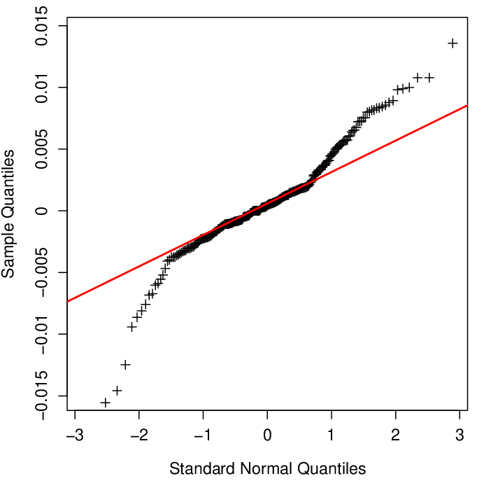
Here we consider the returns of the Hang Seng index over 260260 working days from Jan. 2017 to Nov. 2017 (excluding weekends and public holidays). Figure 4 shows the quantile-quantile (QQ) plot of these returns. The deviation from the straight red line indicates that the returns are significantly non-Gaussian and heavy-tailed.
Refer to caption
Fig. 4: Quantile-quantile plot of the the Hang Seng index returns showing that they are heavy-tailed.

We divide the 260260 returns into two parts: the estimation data, which involves the first 250250 samples, and the test data, which involves the remaining 1010 samples. First, we fit the estimation data to the Gaussian AR(1) model and the Student’s tt AR(1) model, and estimate the parameters. Then we predict the test data using the one-step-ahead predication method based on the estimates, and compute the averaged prediction errors. Next, we randomly delete 1010 of the estimation data, and estimate the parameters of the Gaussian AR(1) model and the Student’s tt AR(1) model from this incomplete data set. Finally, we also make predictions and compute the averaged prediction errors based on these estimates of the parameters. The result is summarized in Table III. We have the following conclusions: i) the Student’s tt AR(1) model performs better than the Gaussian AR(1) model for this heavy-tailed time series, ii) the proposed parameter estimation method for incomplete Student’s tt AR(1) time series can provide similar estimates to the result of complete data.

VII Conclusions

In this paper, we have considered parameter estimation of the heavy-tailed AR model with missing values. We have formulated an ML estimation problem and developed an efficient approach to obtain the estimates based on the stochastic EM. Since the conditional distribution of the latent data in our case is complicated, we proposed a Gibbs sampling scheme to draw realizations from it. The convergence of the proposed algorithm to the stationary points has been established. Simulations show that the proposed approach can provide reliable estimates from incomplete time series with different percentages of missing values, and is robust to outliers. Although in this paper we only focus on the univariate AR model with the Student’s tt distributed innovations due to the limit of the space, our method can be extended to multivariate AR model and also other heavy-tailed distributed innovations.

Appendix A Proof for Lemmas 1 and 2

A-A Proof for Lemma 1

The conditional distribution of 𝝉|𝐲𝗆,𝐲𝗈;𝜽\boldsymbol{\tau}|\mathbf{y}_{\mathsf{m}},\mathbf{y}_{\mathsf{o}};\boldsymbol{\theta} is

p⁡(𝝉|𝐲𝗆,𝐲𝗈;𝜽)\displaystyle p\left(\boldsymbol{\tau}|\mathbf{y}_{\mathsf{m}},\mathbf{y}_{\mathsf{o}};\boldsymbol{\theta}\right) (48)
=p⁡(𝐲,𝝉,𝜽)p⁡(𝐲,𝜽)\displaystyle=\frac{p\left(\mathbf{y},\boldsymbol{\tau};\boldsymbol{\theta}\right)}{p\left(\mathbf{y};\boldsymbol{\theta}\right)}
∝p⁡(𝐲,𝝉,𝜽)\displaystyle\propto p\left(\mathbf{y},\boldsymbol{\tau};\boldsymbol{\theta}\right)
=∏t=2T(ν2)ν2​τtν−12Γ⁡(ν2)​2​π​σ2​exp⁡(−τt2​σ2​(yt−φ0−φ1​yt−1)2−ν2​τt)\displaystyle=\prod_{t=2}^{T}\frac{\left(\frac{\nu}{2}\right)^{\frac{\nu}{2}}\tau_{t}^{\frac{\nu-1}{2}}}{\Gamma\left(\frac{\nu}{2}\right)\sqrt{2\pi\sigma^{2}}}\exp\left(-\frac{\tau_{t}}{2\sigma^{2}}\left(y_{t}-\varphi_{0}-\varphi_{1}y_{t-1}\right)^{2}-\frac{\nu}{2}\tau_{t}\right)
∝∏t=2Tτtν−12​exp⁡(−((yt−φ0−φ1​yt−1)22​σ2+ν2)​τt),\displaystyle\propto\prod_{t=2}^{T}\tau_{t}^{\frac{\nu-1}{2}}\exp\left(-\left(\frac{\left(y_{t}-\varphi_{0}-\varphi_{1}y_{t-1}\right)^{2}}{2\sigma^{2}}+\frac{\nu}{2}\right)\tau_{t}\right),

which implies that {τt}\left\{\tau_{t}\right\} are independent from each other with

p⁡(τt|𝐲𝗆,𝐲𝗈;𝜽)\displaystyle p\left(\tau_{t}|\mathbf{y}_{\mathsf{m}},\mathbf{y}_{\mathsf{o}};\boldsymbol{\theta}\right) (49)
∝τtν−12​exp⁡(−((yt−φ0−φ1​yt−1)22​σ2+ν2)​τt).\displaystyle\propto\tau_{t}^{\frac{\nu-1}{2}}\exp\left(-\left(\frac{\left(y_{t}-\varphi_{0}-\varphi_{1}y_{t-1}\right)^{2}}{2\sigma^{2}}+\frac{\nu}{2}\right)\tau_{t}\right).

Comparing this expression with the pdf of the gamma distribution, we get that τt|𝐲𝗆,𝐲𝗈;𝜽\tau_{t}|\mathbf{y}_{\mathsf{m}},\mathbf{y}_{\mathsf{o}};\boldsymbol{\theta} follows a gamma distribution:

τt|𝐲𝗆,𝐲𝗈;𝜽\displaystyle\tau_{t}|\mathbf{y}_{\mathsf{m}},\mathbf{y}_{\mathsf{o}};\boldsymbol{\theta} (50)
∼G​a​m​m​a​(ν+12,(yt−φ0−φ1​yt−1)2/σ2+ν2).\displaystyle\sim Gamma\left(\frac{\nu+1}{2},\thinspace\frac{\left(y_{t}-\varphi_{0}-\varphi_{1}y_{t-1}\right)^{2}/\sigma^{2}+\nu}{2}\right).

A-B Proof for Lemma 2

According to the Gaussian mixture representation (11) and (12), given 𝝉\boldsymbol{\tau} and 𝜽\boldsymbol{\theta}, εt\varepsilon_{t} follows a Gaussian distribution: εt​∼i.i.d.​𝒩​(μ,σ2τt)\varepsilon_{t}\overset{i.i.d.}{\sim}\mathcal{N}\left(\mu,\frac{\sigma^{2}}{\tau_{t}}\right). From equation (2), we can see that, given 𝝉\boldsymbol{\tau} and 𝜽\boldsymbol{\theta}, the distribution of yty_{t} conditional on all the preceding data ℱt−1,\mathcal{F}_{t-1}, only depends on the previous sample yt−1y_{t-1}:

p⁡(yt|𝝉,ℱt−1;𝜽)=\displaystyle p\left(y_{t}|\boldsymbol{\tau},\mathcal{F}_{t-1};\boldsymbol{\theta}\right)= p⁡(yt|𝝉,yt−1;𝜽).\displaystyle p\left(y_{t}|\boldsymbol{\tau},y_{t-1};\boldsymbol{\theta}\right). (51)

In addition, the distribution of yty_{t} conditional on all the preceding observed data ℱt−1o\mathcal{F}_{t-1}^{o}, 𝝉\boldsymbol{\tau}, and 𝜽\boldsymbol{\theta}, only depends on the nearest observed sample:

p⁡(yt|𝝉,ℱt−1o;𝜽)\displaystyle p\left(y_{t}|\boldsymbol{\tau},\mathcal{F}_{t-1}^{o};\boldsymbol{\theta}\right) (52)
={p⁡(yt|𝝉,yt−1;𝜽)t=td+nd+2,…,td+1,f​o​r​d=0,1,…,D,p⁡(yt|𝝉,yt−nd−1;𝜽)t=td+nd+1,ford=1,2,…,D.\displaystyle=\begin{cases}p\left(y_{t}|\boldsymbol{\tau},y_{t-1};\boldsymbol{\theta}\right)&t=t_{d}+n_{d}+2,\ldots,t_{d+1},\\ &for\thinspace d=0,1,\ldots,D,\\ p\left(y_{t}|\boldsymbol{\tau},y_{t-n_{d}-1};\boldsymbol{\theta}\right)&t=t_{d}+n_{d}+1,for\thinspace d=1,2,\ldots,D.\end{cases}

The first case refers to the situation where the previous sample yt−1y_{t-1} is observed, while the second case is when yt−1y_{t-1} is missing.

Based on the above properties, we have

p⁡(𝐲𝗆|𝝉,𝐲𝗈;𝜽)=\displaystyle p\left(\mathbf{y}_{\mathsf{m}}|\boldsymbol{\tau},\mathbf{y}_{\mathsf{o}};\boldsymbol{\theta}\right)= ∏t=2Tp⁡(yt|𝝉,ℱt−1;𝜽)∏t∈Cop⁡(yt|𝝉,ℱt−1o;𝜽)\displaystyle\frac{\prod_{t=2}^{T}p\left(y_{t}|\boldsymbol{\tau},\mathcal{F}_{t-1};\boldsymbol{\theta}\right)}{\prod_{t\in C_{o}}p\left(y_{t}|\boldsymbol{\tau},\mathcal{F}_{t-1}^{o};\boldsymbol{\theta}\right)} (53a)
=\displaystyle= ∏t=2Tp⁡(yt|𝝉,yt−1;𝜽)∏d=0D∏t=td+nd+2td+1p⁡(yt|𝝉,yt−1;𝜽)\displaystyle\frac{\prod_{t=2}^{T}p\left(y_{t}|\boldsymbol{\tau},y_{t-1};\boldsymbol{\theta}\right)}{\prod_{d=0}^{D}\prod_{t=t_{d}+n_{d}+2}^{t_{d+1}}p\left(y_{t}|\boldsymbol{\tau},y_{t-1};\boldsymbol{\theta}\right)}
×1∏d=1Dp⁡(ytd+nd+1|𝝉,ytd;𝜽)\displaystyle\times\frac{1}{\prod_{d=1}^{D}p\left(y_{t_{d}+n_{d}+1}|\boldsymbol{\tau},y_{t_{d}};\boldsymbol{\theta}\right)} (53b)
=\displaystyle= ∏d=1D∏t=td+1td+nd+1p⁡(yt|𝝉,yt−1;𝜽)∏d=1Dp⁡(ytd+nd+1|𝝉,ytd;𝜽)\displaystyle\frac{\prod_{d=1}^{D}\prod_{t=t_{d}+1}^{t_{d}+n_{d}+1}p\left(y_{t}|\boldsymbol{\tau},y_{t-1};\boldsymbol{\theta}\right)}{\prod_{d=1}^{D}p\left(y_{t_{d}+n_{d}+1}|\boldsymbol{\tau},y_{t_{d}};\boldsymbol{\theta}\right)} (53c)
=\displaystyle= ∏d=1Dp(𝐲d,ytd+nd+1|𝝉,ytd;𝜽)p⁡(ytd+nd+1|𝝉,ytd;𝜽)\displaystyle\prod_{d=1}^{D}\frac{p\left(\mathbf{y}_{d},y_{t_{d}+n_{d}+1}|\boldsymbol{\tau},y_{t_{d}};\boldsymbol{\theta}\right)}{p\left(y_{t_{d}+n_{d}+1}|\boldsymbol{\tau},y_{t_{d}};\boldsymbol{\theta}\right)} (53d)
=\displaystyle= ∏d=1Dp⁡(𝐲d|𝝉,ytd,ytd+nd+1;𝜽),\displaystyle\prod_{d=1}^{D}p\left(\mathbf{y}_{d}|\boldsymbol{\tau},y_{t_{d}},y_{t_{d}+n_{d}+1};\boldsymbol{\theta}\right), (53e)

where the equations (53a) and (53e) are from the definition of conditional pdf, the equation (53b) is from (51) and (52). The equation (53e) implies that the different missing blocks {𝐲d}\left\{\mathbf{y}_{d}\right\} are independent from each other, and the conditional distribution of 𝐲d\mathbf{y}_{d} only depends on the two nearest observed samples ytdy_{t_{d}} and ytd+nd+1.y_{t_{d}+n_{d}+1}.

To obtain the pdf of the missing block p⁡(𝐲d|𝝉,ytd,ytd+nd+1;𝜽)p\left(\mathbf{y}_{d}|\boldsymbol{\tau},y_{t_{d}},y_{t_{d}+n_{d}+1};\boldsymbol{\theta}\right), we first analyze the joint pdf of the missing block and next observed sample 𝐲c​d=[𝐲dT,ytd+nd+1]T=[ytd+1,ytd+2,…,ytd+nd+1]\mathbf{y}_{cd}=\left[\mathbf{y}_{d}^{T},\thinspace y_{t_{d}+n_{d}+1}\right]^{T}=\left[y_{t_{d}+1},y_{t_{d}+2},\ldots,y_{t_{d}+n_{d}+1}\right]: p⁡(𝐲c​d|𝝉,ytd;𝜽)p\left(\mathbf{y}_{cd}|\boldsymbol{\tau},y_{t_{d}};\boldsymbol{\theta}\right). Given 𝝉\boldsymbol{\tau}, ytdy_{t_{d}}, and 𝜽\boldsymbol{\theta}, from (2), we have

ytd+i=\displaystyle y_{t_{d}+i}= φ0+φ1​ytd+i−1+εtd+i\displaystyle\varphi_{0}+\varphi_{1}y_{t_{d}+i-1}+\varepsilon_{t_{d}+i} (54)
=\displaystyle= φ0+φ1​(φ0+φ1​ytd+i−2+εtd+i−1)+εtd+i\displaystyle\varphi_{0}+\varphi_{1}\left(\varphi_{0}+\varphi_{1}y_{t_{d}+i-2}+\varepsilon_{t_{d}+i-1}\right)+\varepsilon_{t_{d}+i}
=\displaystyle= φ0+φ1​φ0+φ12​ytd+i−2+φ1​εtd+i−1+εtd+i\displaystyle\varphi_{0}+\varphi_{1}\varphi_{0}+\varphi_{1}^{2}y_{t_{d}+i-2}+\varphi_{1}\varepsilon_{t_{d}+i-1}+\varepsilon_{t_{d}+i}
=\displaystyle= ∑q=0i−1φ1q​φ0+φ1i​ytd+∑q=1iφ1(i−q)​εtd+q,\displaystyle\sum_{q=0}^{i-1}\varphi_{1}^{q}\varphi_{0}+\varphi_{1}^{i}y_{t_{d}}+\sum_{q=1}^{i}\varphi_{1}^{\left(i-q\right)}\varepsilon_{t_{d}+q},

for i=1,2,…i=1,2,\ldots,nd+1n_{d}+1, which means that ytd+iy_{t_{d}+i} can be expressed as the sum of the constant ∑q=0i−1φ1q​φ0+φ1i​ytd\sum_{q=0}^{i-1}\varphi_{1}^{q}\varphi_{0}+\varphi_{1}^{i}y_{t_{d}} and a linear combination of the independent Gaussian random variables εtd+1,\varepsilon_{t_{d}+1}, εtd+2\varepsilon_{t_{d}+2}, …\ldots, εtd+i.\varepsilon_{t_{d}+i}. Therefore, we can obtain that 𝐲c​d\mathbf{y}_{cd} follows a Gaussian distribution as follows:

𝐲c​d|𝝉,ytd;𝜽∼𝒩⁡(𝝁c​d,𝚺c​d),\mathbf{y}_{cd}|\boldsymbol{\tau},y_{t_{d}};\boldsymbol{\theta}\sim\mathcal{N}\left(\boldsymbol{\mu}_{cd},\boldsymbol{\Sigma}_{cd}\right), (55)

where the ii-th component of 𝝁c​d\boldsymbol{\mu}_{cd}

μc​d​(i)=\displaystyle\mu_{cd(i)}= 𝖤⁡[ytd+i]\displaystyle\mathsf{E}\left[y_{t_{d}+i}\right] (56)
=\displaystyle= 𝖤⁡[∑q=0i−1φ1q​φ0+φ1i​ytd+∑q=1iφ1(i−q)​εtd+q]\displaystyle\mathsf{E}\left[\sum_{q=0}^{i-1}\varphi_{1}^{q}\varphi_{0}+\varphi_{1}^{i}y_{t_{d}}+\sum_{q=1}^{i}\varphi_{1}^{\left(i-q\right)}\varepsilon_{t_{d}+q}\right]
=\displaystyle= ∑q=0i−1φ1q​φ0+φ1i​ytd+∑q=1iφ1(i−q)​𝖤​[εtd+q]\displaystyle\sum_{q=0}^{i-1}\varphi_{1}^{q}\varphi_{0}+\varphi_{1}^{i}y_{t_{d}}+\sum_{q=1}^{i}\varphi_{1}^{\left(i-q\right)}\mathsf{E}\left[\varepsilon_{t_{d}+q}\right]
=\displaystyle= ∑q=0i−1φ1q​φ0+φ1i​ytd,\displaystyle\sum_{q=0}^{i-1}\varphi_{1}^{q}\varphi_{0}+\varphi_{1}^{i}y_{t_{d}},

and the component in the ii-th column and the jj-th row of 𝚺c​d\boldsymbol{\Sigma}_{cd}

Σc​d​(i,j)=\displaystyle\Sigma_{cd(i,j)}= 𝖤⁡[(ytd+i−μc​d​(i))​(ytd+j−μc​d​(j))]\displaystyle\mathsf{E}\left[\left(y_{t_{d}+i}-\mu_{cd(i)}\right)\left(y_{t_{d}+j}-\mu_{cd(j)}\right)\right] (57)
=\displaystyle= 𝖤⁡[(∑q1=1iφ1(i−q1)​εtd+q1)​(∑q2=1jφ1(j−q2)​εtd+q2)]\displaystyle\mathsf{E}\left[\left(\sum_{q_{1}=1}^{i}\varphi_{1}^{\left(i-q_{1}\right)}\varepsilon_{t_{d}+q_{1}}\right)\left(\sum_{q_{2}=1}^{j}\varphi_{1}^{\left(j-q_{2}\right)}\varepsilon_{t_{d}+q_{2}}\right)\right]
=\displaystyle= ∑q1=1i∑q2=1jφ1(i+j−q1−q2)​𝖤​[εtd+q1​εtd+q2]\displaystyle\sum_{q_{1}=1}^{i}\sum_{q_{2}=1}^{j}\varphi_{1}^{\left(i+j-q_{1}-q_{2}\right)}\mathsf{E}\left[\varepsilon_{t_{d}+q_{1}}\varepsilon_{t_{d}+q_{2}}\right]
=\displaystyle= σ2​∑q=1min⁡(i,j)φ1(i+j−2​q)τtd+q.\displaystyle\sigma^{2}\sum_{q=1}^{\min\left(i,j\right)}\frac{\varphi_{1}^{\left(i+j-2q\right)}}{\tau_{t_{d}+q}}.

with the last equation following from

𝖤⁡[εtd+q1​εtd+q2]={σ2τtd+q1,q1=q2;0,q1≠q2.\mathsf{E}\left[\varepsilon_{t_{d}+q_{1}}\varepsilon_{t_{d}+q_{2}}\right]=\begin{cases}\frac{\sigma^{2}}{\tau_{t_{d}+q_{1}}},&q_{1}=q_{2};\\ 0,&q_{1}\neq q_{2}.\end{cases}

Recall that p⁡(𝐲d|𝝉,ytd,ytd+nd+1;𝜽)p\left(\mathbf{y}_{d}|\boldsymbol{\tau},y_{t_{d}},y_{t_{d}+n_{d}+1};\boldsymbol{\theta}\right) is a conditional pdf of p(𝐲d,ytd+nd+1|𝝉,ytd;𝜽)p\left(\mathbf{y}_{d},y_{t_{d}+n_{d}+1}|\boldsymbol{\tau},y_{t_{d}};\boldsymbol{\theta}\right). Since conditional distributions of a Gaussian distribution is Gaussian, we can get that 𝐲d|𝝉,ytd,ytd+nd+1;𝜽\mathbf{y}_{d}|\boldsymbol{\tau},y_{t_{d}},y_{t_{d}+n_{d}+1};\boldsymbol{\theta} follows a Gaussian distribution as (28). The parameters of this conditional distribution can be computed based on

𝝁d=𝝁c​d​(1:nd)+𝚺cd(1:nd,nd+1)Σc​d​(nd+1,nd+1)(ytd+nd+1−μc​d​(nd+1)),\mathbf{\boldsymbol{\mu}}_{d}=\boldsymbol{\mu}_{cd(1:n_{d})}+\frac{\boldsymbol{\Sigma}_{cd(1:n_{d},n_{d}+1)}}{\Sigma_{cd(n_{d}+1,n_{d}+1)}}\left(y_{t_{d}+n_{d}+1}-\mu_{cd(n_{d}+1)}\right), (58)

and

𝚺d=𝚺cd(1:nd,1:nd)−𝚺cd(1:nd,nd+1)𝚺cd(nd+1,1:nd)Σc​d​(nd+1,nd+1),\boldsymbol{\Sigma}_{d}=\boldsymbol{\Sigma}_{cd(1:n_{d},1:n_{d})}-\frac{\boldsymbol{\Sigma}_{cd(1:n_{d},n_{d}+1)}\boldsymbol{\Sigma}_{cd(n_{d}+1,1:n_{d})}}{\Sigma_{cd(n_{d}+1,n_{d}+1)}}, (59)

where 𝝁c​d​(a1:a2)\boldsymbol{\mu}_{cd(a_{1}:a_{2})} denotes the subvector consisting of the a1a_{1}-th to a2a_{2}-th component of 𝝁c​d\mathbf{\boldsymbol{\mu}}_{cd}, and the 𝚺cd(a1:a2,b1:b2)\boldsymbol{\Sigma}_{cd(a_{1}:a_{2},b_{1}:b_{2})} means the submatrix consisting of the components in the a1a_{1}-th to a2a_{2}-th rows and the b​1b1-th to b2b_{2}-th columns of 𝚺c​d\boldsymbol{\Sigma}_{cd}. Plugging the equations (56) and (57) into the equations (58) and (59) gives the equations (29) and (30), respectively.

Appendix B Proof for Conditions (M1)-(M5) and (SAEM2)-(SAEM3)

In this section, we will establish the listed conditions one by one. The observed data 𝐲𝗈\mathbf{y}_{\mathsf{o}} is known. We assume that 𝐲𝗈\mathbf{y}_{\mathsf{o}} is finite. Since the parameter space Θ\Theta is a large bounded set with ν>2\nu>2, we can assume that |φ0|<φ0+,|φ1|​<φ1+,σ>​σ−,|\varphi_{0}|<\varphi_{0}^{+},|\varphi_{1}|<\varphi_{1}^{+},\sigma>\sigma^{-}, and ν−<ν<ν+\nu^{-}<\nu<\nu^{+}, where φ0+\varphi_{0}^{+}, φ1+\varphi_{1}^{+}, and ν+\nu^{+} are very large positive numbers, σ−\sigma^{-} is a very small positive number, and ν−\nu^{-} is a very small positive number satisfying ν−≥2\nu^{-}\geq 2. We first prove the conditions (M1)-(M5), then prove the conditions (SAEM2) and (SAEM3).

B-A Proof of (M1)-(M5)

The proof begins by establishing the following two intermediary lemmas.

Lemma 3.

For any 𝐲𝗈\mathbf{y}_{\mathsf{o}} and 𝜽∈Θ\boldsymbol{\theta}\in\Theta, p⁡(𝐲𝗈,𝜽)=∫∫⁡p⁡(𝐲,𝝉,𝜽)​𝖽​𝐲𝗆​𝑑𝝉=∫p⁡(𝐲,𝜽)​𝖽​𝐲𝗆<∞.p\left(\mathbf{y}_{\mathsf{o}};\boldsymbol{\theta}\right)=\int\int p\left(\mathbf{y},\boldsymbol{\tau};\boldsymbol{\theta}\right)\mathsf{d}\mathbf{y}_{\mathsf{m}}\mathsf{d\boldsymbol{\tau}}=\int p\left(\mathbf{y};\boldsymbol{\theta}\right)\mathsf{d}\mathbf{y}_{\mathsf{m}}<\infty.

Lemma 4.

For any 𝐲𝗈\mathbf{y}_{\mathsf{o}} , 𝛉∈Θ\boldsymbol{\theta}\in\Theta and 1<t≤T1<t\leq T

∬g⁡(𝐲,𝝉)​p​(𝐲,𝝉,𝜽)​𝖽​𝐲𝗆​𝑑𝝉<∞,\iint g\left(\mathbf{y},\boldsymbol{\tau}\right)p\left(\mathbf{y},\boldsymbol{\tau};\boldsymbol{\theta}\right)\mathsf{d}\mathbf{y}_{\mathsf{m}}\mathsf{d\boldsymbol{\tau}}<\infty, (60)

where g⁡(𝐲,𝛕)g\left(\mathbf{y},\boldsymbol{\tau}\right) can be τt\tau_{t}, τt2\tau_{t}^{2}, yt2y_{t}^{2},τt​yt−12\tau_{t}y_{t-1}^{2}, τt​yt2\tau_{t}y_{t}^{2}, or −log⁡(τt)-\log\left(\tau_{t}\right)

Lemma 3 indicates that the observed data likelihood p⁡(𝐲𝗈,𝜽)p\left(\mathbf{y}_{\mathsf{o}};\boldsymbol{\theta}\right) is bounded, and Lemma 4 shows that the expectation of g⁡(𝐲,𝝉)g\left(\mathbf{y},\boldsymbol{\tau}\right) is bounded. These lemmas provide the key ingredients required for establishing (M1)-(M5), and their usage for subsequent analysis is self-explanatory. Due to space limitations, we do not include their proofs here. Interested readers may refer to the supplementary material.

(M1) For condition (M1), based on (18), we can get

∫∫∥𝐬(𝐲𝗈,𝐲𝗆,𝝉)∥p(𝐲𝗆,𝝉|𝐲𝗈;𝜽)𝖽𝐲𝗆𝖽𝝉\displaystyle\int\int\|\mathbf{s}\left(\mathbf{y}_{\mathsf{o}},\mathbf{y}_{\mathsf{m}},\boldsymbol{\tau}\right)\|p\left(\mathbf{y}_{\mathsf{m}},\boldsymbol{\tau}|\mathbf{y}_{\mathsf{o}};\boldsymbol{\theta}\right)\mathsf{d}\mathbf{y}_{\mathsf{m}}\mathsf{d\boldsymbol{\tau}} (61)
=∫∫⁡‖𝐬⁡(𝐲𝗈,𝐲𝗆,𝝉)‖​p​(𝐲𝗈,𝐲𝗆,𝝉,𝜽)​𝖽​𝐲𝗆​𝑑𝝉p⁡(𝐲𝗈,𝜽)\displaystyle=\frac{\int\int\|\mathbf{s}\left(\mathbf{y}_{\mathsf{o}},\mathbf{y}_{\mathsf{m}},\boldsymbol{\tau}\right)\|p\left(\mathbf{y}_{\mathsf{o}},\mathbf{y}_{\mathsf{m}},\boldsymbol{\tau};\boldsymbol{\theta}\right)\mathsf{d}\mathbf{y}_{\mathsf{m}}\mathsf{d\boldsymbol{\tau}}}{p\left(\mathbf{y}_{\mathsf{o}};\boldsymbol{\theta}\right)}
≤1p⁡(𝐲𝗈,𝜽)​∑t=2T∫∫⁡(|log⁡(τt)−τt|+|τt​yt2|+|τt|CLOSE\displaystyle\leq\frac{1}{p\left(\mathbf{y}_{\mathsf{o}};\boldsymbol{\theta}\right)}\sum_{t=2}^{T}\int\int\biggl(\bigr|\log\left(\tau_{t}\right)-\tau_{t}\bigr|+\bigr|\tau_{t}y_{t}^{2}\bigr|+\bigr|\tau_{t}\bigr|
+|τt​yt−12|+|τt​yt|+|τt​yt​yt−1|\displaystyle+\bigr|\tau_{t}y_{t-1}^{2}\bigr|+\bigr|\tau_{t}y_{t}\bigr|+\bigr|\tau_{t}y_{t}y_{t-1}\bigr|
OPEN+|τt​yt−1|)​p​(𝐲𝗈,𝐲𝗆,𝝉,𝜽)​𝖽​𝐲𝗆​𝖽​𝝉\displaystyle+\bigr|\tau_{t}y_{t-1}\bigr|\biggr)p\left(\mathbf{y}_{\mathsf{o}},\mathbf{y}_{\mathsf{m}},\boldsymbol{\tau};\boldsymbol{\theta}\right)\mathsf{d}\mathbf{y}_{\mathsf{m}}\mathsf{d\boldsymbol{\tau}}
≤1p⁡(𝐲𝗈,𝜽)​∑t=2T∫∫⁡(τt−log⁡(τt)+τt​yt2+τtCLOSE\displaystyle\leq\frac{1}{p\left(\mathbf{y}_{\mathsf{o}};\boldsymbol{\theta}\right)}\sum_{t=2}^{T}\int\int\biggl(\tau_{t}-\log\left(\tau_{t}\right)+\tau_{t}y_{t}^{2}+\tau_{t}
+τt​yt−12+τt2+yt22+τt​(yt2+yt−12)2\displaystyle+\tau_{t}y_{t-1}^{2}+\frac{\tau_{t}^{2}+y_{t}^{2}}{2}+\frac{\tau_{t}\left(y_{t}^{2}+y_{t-1}^{2}\right)}{2}
OPEN+τt2+yt−122)​p​(𝐲𝗈,𝐲𝗆,𝝉,𝜽)​𝖽​𝐲𝗆​𝖽​𝝉\displaystyle+\frac{\tau_{t}^{2}+y_{t-1}^{2}}{2}\biggr)p\left(\mathbf{y}_{\mathsf{o}},\mathbf{y}_{\mathsf{m}},\boldsymbol{\tau};\boldsymbol{\theta}\right)\mathsf{d}\mathbf{y}_{\mathsf{m}}\mathsf{d\boldsymbol{\tau}}
<∞,\displaystyle<\infty,

where the three inequalities follow from the triangular inequality, the property of squares x1​x2≤x12+x222x_{1}x_{2}\leq\frac{x_{1}^{2}+x_{2}^{2}}{2}, and Lemma 4, respectively.

(M2) From the definition of ψ⁡(𝜽)\psi\left(\boldsymbol{\theta}\right) and ϕ⁡(𝜽)\boldsymbol{\phi}\left(\boldsymbol{\theta}\right) in (16) and (17), their continuous differentiability can be easily verified.

(M3) For condition (M3),

𝐬¯​(𝜽)=\displaystyle\bar{\mathbf{s}}\left(\boldsymbol{\theta}\right)= ∫∫𝐬(𝐲𝗈,𝐲𝗆,𝝉)p(𝐲𝗆,𝝉|𝐲𝗈;𝜽)𝖽𝐲𝗆𝖽𝝉\displaystyle\int\int\mathbf{s}\left(\mathbf{y}_{\mathsf{o}},\mathbf{y}_{\mathsf{m}},\boldsymbol{\tau}\right)p\left(\mathbf{y}_{\mathsf{m}},\boldsymbol{\tau}|\mathbf{y}_{\mathsf{o}};\boldsymbol{\theta}\right)\mathsf{d}\mathbf{y}_{\mathsf{m}}\mathsf{d\boldsymbol{\tau}} (62)
=\displaystyle= ∫∫⁡𝐬⁡(𝐲𝗈,𝐲𝗆,𝝉)​p⁡(𝐲,𝝉,𝜽)p⁡(𝐲𝗈,𝜽)​𝖽​𝐲𝗆​𝖽𝝉\displaystyle\int\int\mathbf{s}\left(\mathbf{y}_{\mathsf{o}},\mathbf{y}_{\mathsf{m}},\boldsymbol{\tau}\right)\frac{p\left(\mathbf{y},\boldsymbol{\tau};\boldsymbol{\theta}\right)}{p\left(\mathbf{y}_{\mathsf{o}};\boldsymbol{\theta}\right)}\mathsf{d}\mathbf{y}_{\mathsf{m}}\mathsf{d\boldsymbol{\tau}}
=\displaystyle= ∫∫⁡𝐬⁡(𝐲𝗈,𝐲𝗆,𝝉)​p​(𝐲,𝝉,𝜽)​𝖽​𝐲𝗆​𝑑𝝉∫∫⁡p⁡(𝐲,𝝉,𝜽)​𝖽​𝐲𝗆​𝑑𝝉.\displaystyle\frac{\int\int\mathbf{s}\left(\mathbf{y}_{\mathsf{o}},\mathbf{y}_{\mathsf{m}},\boldsymbol{\tau}\right)p\left(\mathbf{y},\boldsymbol{\tau};\boldsymbol{\theta}\right)\mathsf{d}\mathbf{y}_{\mathsf{m}}\mathsf{d\boldsymbol{\tau}}}{\int\int p\left(\mathbf{y},\boldsymbol{\tau};\boldsymbol{\theta}\right)\mathsf{d}\mathbf{y}_{\mathsf{m}}\mathsf{d\boldsymbol{\tau}}}.

Since ∫∫⁡p⁡(𝐲,𝝉,𝜽)​𝖽​𝐲𝗆​𝑑𝝉=p⁡(𝐲𝗈,𝜽)>0\int\int p\left(\mathbf{y},\boldsymbol{\tau};\boldsymbol{\theta}\right)\mathsf{d}\mathbf{y}_{\mathsf{m}}\mathsf{d\boldsymbol{\tau}}=p\left(\mathbf{y}_{\mathsf{o}};\boldsymbol{\theta}\right)>0 and p⁡(𝐲,𝝉,𝜽)p\left(\mathbf{y},\boldsymbol{\tau};\boldsymbol{\theta}\right) is continuously differentiable, which can be easily checked from its definition (19), we can get that 𝐬¯​(𝜽)\bar{\mathbf{s}}\left(\boldsymbol{\theta}\right) is continuously differentiable.

(M4) Since ∫∫⁡p⁡(𝐲,𝝉,𝜽)​𝖽​𝐲𝗆​𝑑𝝉>0\int\int p\left(\mathbf{y},\boldsymbol{\tau};\boldsymbol{\theta}\right)\mathsf{d}\mathbf{y}_{\mathsf{m}}\mathsf{d\boldsymbol{\tau}}>0, and p⁡(𝐲,𝝉,𝜽)p\left(\mathbf{y},\boldsymbol{\tau};\boldsymbol{\theta}\right) is 7 times differentiable, l⁡(𝜽,𝐲𝗈)=log⁡(∫∫⁡p⁡(𝐲,𝝉,𝜽)​𝖽​𝐲𝗆​𝑑𝝉)l\left(\boldsymbol{\theta};\mathbf{y}_{\mathsf{o}}\right)=\log\left(\int\int p\left(\mathbf{y},\boldsymbol{\tau};\boldsymbol{\theta}\right)\mathsf{d}\mathbf{y}_{\mathsf{m}}\mathsf{d\boldsymbol{\tau}}\right) is 7 times differentiable. For the verification of the equation (46), according to Leibniz integral rule, the equation (46) holds under the following three conditions:

  1. 1.

    ∫∫⁡p⁡(𝐲,𝝉,𝜽)​𝖽​𝐲𝗆​𝑑𝝉<∞\int\int p\left(\mathbf{y},\boldsymbol{\tau};\boldsymbol{\theta}\right)\mathsf{d}\mathbf{y}_{\mathsf{m}}\mathsf{d\boldsymbol{\tau}}<\infty,

  2. 2.

    ∂p⁡(𝐲,𝝉,𝜽)∂𝜽\frac{\partial p\left(\mathbf{y},\boldsymbol{\tau};\boldsymbol{\theta}\right)}{\partial\boldsymbol{\theta}} exists for all the 𝜽∈Θ\boldsymbol{\theta}\in\Theta,

  3. 3.

    there is an integrable function g⁡(𝐲,𝝉)g\left(\mathbf{y},\boldsymbol{\tau}\right) such that |\Bigl|∂p⁡(𝐲,𝝉,𝜽)∂𝜽|≤g⁡(𝐲,𝝉)\frac{\partial p\left(\mathbf{y},\boldsymbol{\tau};\boldsymbol{\theta}\right)}{\partial\boldsymbol{\theta}}\Bigr|\leq g\left(\mathbf{y},\boldsymbol{\tau}\right) for all 𝜽∈Θ\boldsymbol{\theta}\in\Theta and almost every 𝐲\mathbf{y} and 𝝉\boldsymbol{\tau}.

Since the first condition has been proved in Lemma 3, and the second condition can be easily verified from its definition, here we focus on the third condition.

From the equation (13), the derivative of p⁡(𝐲,𝝉,𝜽)p\left(\mathbf{y},\boldsymbol{\tau};\boldsymbol{\theta}\right) with respect to φ0\varphi_{0} is

|∂p⁡(𝐲,𝝉,𝜽)∂φ0|\displaystyle\biggl|\frac{\partial p\left(\mathbf{y},\boldsymbol{\tau};\boldsymbol{\theta}\right)}{\partial\varphi_{0}}\biggl| (63)
=|p⁡(𝐲,𝝉,𝜽)​∑j=2Tτj​(yj−φ0−φ1​yj−1)σ2|\displaystyle=\Biggl|p\left(\mathbf{y},\boldsymbol{\tau};\boldsymbol{\theta}\right)\sum_{j=2}^{T}\frac{\tau_{j}\left(y_{j}-\varphi_{0}-\varphi_{1}y_{j-1}\right)}{\sigma^{2}}\Biggr|
≤p⁡(𝐲,𝝉,𝜽)σ2​∑j=2T(|τj​yj|+|φ0​τj|+|φ1​τj​yj−1|)\displaystyle\leq\frac{p\left(\mathbf{y},\boldsymbol{\tau};\boldsymbol{\theta}\right)}{\sigma^{2}}\sum_{j=2}^{T}\left(|\tau_{j}y_{j}|+|\varphi_{0}\tau_{j}|+|\varphi_{1}\tau_{j}y_{j-1}|\right)
≤p⁡(𝐲,𝝉,𝜽∗)(σ−)2​∑j=2T{(τj2+yj22+φ0+​τj+φ1+​(yj−12+τj2)2)}\displaystyle\leq\frac{p\left(\mathbf{y},\boldsymbol{\tau};\boldsymbol{\theta}^{\ast}\right)}{\left(\sigma^{-}\right)^{2}}\sum_{j=2}^{T}\biggl\{\biggl(\frac{\tau_{j}^{2}+y_{j}^{2}}{2}+\varphi_{0}^{+}\tau_{j}+\frac{\varphi_{1}^{+}\left(y_{j-1}^{2}+\tau_{j}^{2}\right)}{2}\biggr)\biggr\}
=gφ0​(𝐲,𝝉),\displaystyle=g_{\varphi_{0}}\left(\mathbf{y},\boldsymbol{\tau}\right),

where 𝜽∗=arg⁡max𝜽∈Θ​p​(𝐲,𝝉,𝜽).\boldsymbol{\theta}^{*}=\underset{\boldsymbol{\theta}\in\Theta}{\arg\max\ }p\left(\mathbf{y},\boldsymbol{\tau};\boldsymbol{\theta}\right). The first inequality follows from the triangle inequality, and the second inequality follows from p⁡(𝐲,𝝉,𝜽∗)≥p⁡(𝐲,𝝉,𝜽)p\left(\mathbf{y},\boldsymbol{\tau};\boldsymbol{\theta}^{\ast}\right)\geq p\left(\mathbf{y},\boldsymbol{\tau};\boldsymbol{\theta}\right), |φ0|<φ0+|\varphi_{0}|<\varphi_{0}^{+}, |φ1|<φ1+|\varphi_{1}|<\varphi_{1}^{+}, σ>σ−\sigma>\sigma^{-}, and the property of squares.

The derivative with respect to φ1\varphi_{1} is

|∂p⁡(𝐲,𝝉,𝜽)∂φ1|\displaystyle\biggl|\frac{\partial p\left(\mathbf{y},\boldsymbol{\tau};\boldsymbol{\theta}\right)}{\partial\varphi_{1}}\biggl|
=|p⁡(𝐲,𝝉,𝜽)​∑j=2T1σ2​τj​yj−1​(yj−φ0−φ1​yj−1)|\displaystyle=\biggr|p\left(\mathbf{y},\boldsymbol{\tau};\boldsymbol{\theta}\right)\sum_{j=2}^{T}\frac{1}{\sigma^{2}}\tau_{j}y_{j-1}\left(y_{j}-\varphi_{0}-\varphi_{1}y_{j-1}\right)\biggr|\hskip 40.00006pt
≤p⁡(𝐲,𝝉,𝜽)σ2​∑j=2T(|τj​yj​yj−1|+|φ0​τj​yj−1|+|φ1​τj​yj−12|)\displaystyle\leq\frac{p\left(\mathbf{y},\boldsymbol{\tau};\boldsymbol{\theta}\right)}{\sigma^{2}}\sum_{j=2}^{T}\biggl(|\tau_{j}y_{j}y_{j-1}|+|\varphi_{0}\tau_{j}y_{j-1}|+|\varphi_{1}\tau_{j}y_{j-1}^{2}|\biggr)
≤p⁡(𝐲,𝝉,𝜽∗)(σ−)2​∑j=2T(τj​(yj2+yj−12)2+φ0+​(τj2+yj−12)2CLOSE\displaystyle\leq\frac{p\left(\mathbf{y},\boldsymbol{\tau};\boldsymbol{\theta}^{\ast}\right)}{\left(\sigma^{-}\right)^{2}}\sum_{j=2}^{T}\biggl(\frac{\tau_{j}\left(y_{j}^{2}+y_{j-1}^{2}\right)}{2}+\frac{\varphi_{0}^{+}\left(\tau_{j}^{2}+y_{j-1}^{2}\right)}{2}
OPEN+φ1+​τj​yj−12)\displaystyle\hskip 85.00012pt+\varphi_{1}^{+}\tau_{j}y_{j-1}^{2}\biggr)
=gφ1​(𝐲,𝝉),\displaystyle=g_{\varphi_{1}}\left(\mathbf{y},\boldsymbol{\tau}\right), (64)

where the first inequality follows from the triangle inequality, and the second inequality follows from |φ0|<φ0+|\varphi_{0}|<\varphi_{0}^{+}, |φ1|<φ1+|\varphi_{1}|<\varphi_{1}^{+}, σ>σ−\sigma>\sigma^{-}, and the property of squares.

The derivative with respect to σ2\sigma^{2} is

|∂p⁡(𝐲,𝝉,𝜽)∂σ2|\displaystyle\biggl|\frac{\partial p\left(\mathbf{y},\boldsymbol{\tau};\boldsymbol{\theta}\right)}{\partial\sigma^{2}}\biggl| (65)
=p(𝐲,𝝉;𝜽)∑j=2T{τj2​σ4(yj−φ0−φ1yj−1)2−12​σ2}|\displaystyle=p\left(\mathbf{y},\boldsymbol{\tau};\boldsymbol{\theta}\right)\sum_{j=2}^{T}\left\{\frac{\tau_{j}}{2\sigma^{4}}\left(y_{j}-\varphi_{0}-\varphi_{1}y_{j-1}\right)^{2}-\frac{1}{2\sigma^{2}}\right\}\biggr|
≤p⁡(𝐲,𝝉,𝜽)​∑j=2T{τj2​σ4​(yj−φ0−φ1​yj−1)2+12​σ2}\displaystyle\leq p\left(\mathbf{y},\boldsymbol{\tau};\boldsymbol{\theta}\right)\sum_{j=2}^{T}\left\{\frac{\tau_{j}}{2\sigma^{4}}\left(y_{j}-\varphi_{0}-\varphi_{1}y_{j-1}\right)^{2}+\frac{1}{2\sigma^{2}}\right\}
≤p⁡(𝐲,𝝉,𝜽)​∑j=2T{τj2​σ4​(2​(yj−φ0)2+2​φ12​yj−12)+12​σ2}\displaystyle\leq p\left(\mathbf{y},\boldsymbol{\tau};\boldsymbol{\theta}\right)\sum_{j=2}^{T}\left\{\frac{\tau_{j}}{2\sigma^{4}}\left(2\left(y_{j}-\varphi_{0}\right)^{2}+2\varphi_{1}^{2}y_{j-1}^{2}\right)+\frac{1}{2\sigma^{2}}\right\}
≤p⁡(𝐲,𝝉,𝜽)​∑j=2T{τj2​σ4​(4​yj2+4​φ02+2​φ12​yj−12)+12​σ2}\displaystyle\leq p\left(\mathbf{y},\boldsymbol{\tau};\boldsymbol{\theta}\right)\sum_{j=2}^{T}\left\{\frac{\tau_{j}}{2\sigma^{4}}\left(4y_{j}^{2}+4\varphi_{0}^{2}+2\varphi_{1}^{2}y_{j-1}^{2}\right)+\frac{1}{2\sigma^{2}}\right\}
≤p(𝐲,𝝉;𝜽∗)∑j=2T{τj2​(σ−)2(4yj2+4(φ0+)2+2(φ1+)2yj−12)\displaystyle\leq p\left(\mathbf{y},\boldsymbol{\tau};\boldsymbol{\theta}^{\ast}\right)\sum_{j=2}^{T}\biggl\{\frac{\tau_{j}}{2\left(\sigma^{-}\right)^{2}}\left(4y_{j}^{2}+4\left(\varphi_{0}^{+}\right)^{2}+2\left(\varphi_{1}^{+}\right)^{2}y_{j-1}^{2}\right)
+12​(σ−)2}\displaystyle+\frac{1}{2\left(\sigma^{-}\right)^{2}}\biggr\}
=gσ2​(𝐲,𝝉),\displaystyle=g_{\sigma^{2}}\left(\mathbf{y},\boldsymbol{\tau}\right),

where the first inequality follows from the triangle inequality, the second and third inequalities follow from the property of squares (x1−x2)2≤2​(x12+x22)\left(x_{1}-x_{2}\right)^{2}\leq 2\left(x_{1}^{2}+x_{2}^{2}\right), and the last inequality follows from p⁡(𝐲,𝝉,𝜽∗)≥p⁡(𝐲,𝝉,𝜽)p\left(\mathbf{y},\boldsymbol{\tau};\boldsymbol{\theta}^{\ast}\right)\geq p\left(\mathbf{y},\boldsymbol{\tau};\boldsymbol{\theta}\right), |φ0|<φ0+|\varphi_{0}|<\varphi_{0}^{+}, |φ1|<φ1+|\varphi_{1}|<\varphi_{1}^{+}, and σ>σ−\sigma>\sigma^{-}.

The derivative with respect to ν\nu is

|∂p⁡(𝐲,𝝉,𝜽)∂ν|\displaystyle\biggl|\frac{\partial p\left(\mathbf{y},\boldsymbol{\tau};\boldsymbol{\theta}\right)}{\partial\nu}\biggl| (66)
=|p⁡(𝐲,𝝉,𝜽)​∑j=2T12​(1+log⁡(ν2)−Ψ⁡(ν2)+log⁡(τj)−τj)|\displaystyle=\biggr|p\left(\mathbf{y},\boldsymbol{\tau};\boldsymbol{\theta}\right)\sum_{j=2}^{T}\frac{1}{2}\left(1+\log\left(\frac{\nu}{2}\right)-\Psi\left(\frac{\nu}{2}\right)+\log\left(\tau_{j}\right)-\tau_{j}\right)\biggr|
≤12​p​(𝐲,𝝉,𝜽)​∑j=2T{|1+log⁡(ν2)−Ψ⁡(ν2)|+|log⁡(τj)−τj|}\displaystyle\leq\frac{1}{2}p\left(\mathbf{y},\boldsymbol{\tau};\boldsymbol{\theta}\right)\sum_{j=2}^{T}\left\{\biggr|1+\log\left(\frac{\nu}{2}\right)-\Psi\left(\frac{\nu}{2}\right)\biggr|+\biggr|\log\left(\tau_{j}\right)-\tau_{j}\biggr|\right\}
≤p⁡(𝐲,𝝉,𝜽∗)​∑j=2T(12+12​log⁡(ν−2)−12​Ψ​(ν−2)CLOSE\displaystyle\leq p\left(\mathbf{y},\boldsymbol{\tau};\boldsymbol{\theta}^{\ast}\right)\sum_{j=2}^{T}\biggl(\frac{1}{2}+\frac{1}{2}\log\left(\frac{\nu^{-}}{2}\right)-\frac{1}{2}\Psi\left(\frac{\nu^{-}}{2}\right)
OPEN+12​τj−12​log⁡(τj))\displaystyle+\frac{1}{2}\tau_{j}-\frac{1}{2}\log\left(\tau_{j}\right)\biggr)
=gν​(𝐲,𝝉),\displaystyle=g_{\nu}\left(\mathbf{y},\boldsymbol{\tau}\right),

where Ψ⁡(⋅)\varPsi\left(\cdot\right) is the digamma function. The first inequality follows from the triangle inequality, and the second inequality is due to that log⁡(ν2)−Ψ⁡(ν2)\log\left(\frac{\nu}{2}\right)-\varPsi\left(\frac{\nu}{2}\right) is positive and strictly decreasing for ν≥ν−\nu\geq\nu^{-}[30].

Based on Lemmas 3 and 4, we can obtain that ∬gφ0(𝐲,𝝉,)𝖽𝐲𝗆𝖽𝝉<∞,\iint g_{\varphi_{0}}\left(\mathbf{y},\boldsymbol{\tau},\right)\mathsf{d}\mathbf{y}_{\mathsf{m}}\mathsf{d\boldsymbol{\tau}}<\infty, ∬gφ1​(𝐲,𝝉)​𝖽​𝐲𝗆​𝑑𝝉<∞\iint g_{\varphi_{1}}\left(\mathbf{y},\boldsymbol{\tau}\right)\mathsf{d}\mathbf{y}_{\mathsf{m}}\mathsf{d\boldsymbol{\tau}}<\infty, ∬gσ2​(𝐲,𝝉)​𝖽​𝐲𝗆​𝑑𝝉<∞\iint g_{\sigma^{2}}\left(\mathbf{y},\boldsymbol{\tau}\right)\mathsf{d}\mathbf{y}_{\mathsf{m}}\mathsf{d\boldsymbol{\tau}}<\infty, and ∬gν​(𝐲,𝝉)​𝖽​𝐲𝗆​𝑑𝝉<∞.\iint g_{\nu}\left(\mathbf{y},\boldsymbol{\tau}\right)\mathsf{d}\mathbf{y}_{\mathsf{m}}\mathsf{d\boldsymbol{\tau}}<\infty. The condition (M4) is verified.

(M5) This condition requires the existence of the global maximizer 𝜽~​(𝐬¯)\tilde{\boldsymbol{\theta}}\left(\bar{\mathbf{s}}\right) for Q⁡(𝜽,𝐬¯)Q\left(\boldsymbol{\theta},\bar{\mathbf{s}}\right) and its continuous differentiability. Since Q⁡(𝜽,𝐬¯)Q\left(\boldsymbol{\theta},\bar{\mathbf{s}}\right) takes the same form with Q^​(𝜽,𝐬^(k)),\hat{Q}\left(\boldsymbol{\theta},\hat{\mathbf{s}}^{\left(k\right)}\right), the maximizer will also take the same form. From (34)-(37), we have

φ0~​(𝐬¯)=s¯5−φ1~​(𝐬¯)​s¯7s¯3,\tilde{\varphi_{0}}\left(\bar{\mathbf{s}}\right)=\frac{\bar{s}_{5}-\tilde{\varphi_{1}}\left(\bar{\mathbf{s}}\right)\bar{s}_{7}}{\bar{s}_{3}}, (67)
φ1~​(𝐬¯)=s¯3​s¯6−s¯5​s¯7s¯3​s¯4−s¯72,\tilde{\varphi_{1}}\left(\bar{\mathbf{s}}\right)=\frac{\bar{s}_{3}\bar{s}_{6}-\bar{s}_{5}\bar{s}_{7}}{\bar{s}_{3}\bar{s}_{4}-\bar{s}_{7}^{2}}, (68)
(σ~​(𝐬¯))2=\displaystyle\left(\tilde{\sigma}\left(\bar{\mathbf{s}}\right)\right)^{2}= 1T−1​(s¯2+(φ0~​(𝐬¯))2​s¯3+(φ1~​(𝐬¯))2​s¯4−2​φ0~​(𝐬¯)​s¯5CLOSE\displaystyle\frac{1}{T-1}\biggl(\bar{s}_{2}+\left(\tilde{\varphi_{0}}\left(\bar{\mathbf{s}}\right)\right)^{2}\bar{s}_{3}+\left(\tilde{\varphi_{1}}\left(\bar{\mathbf{s}}\right)\right)^{2}\bar{s}_{4}-2\tilde{\varphi_{0}}\left(\bar{\mathbf{s}}\right)\bar{s}_{5} (69)
OPEN−2​φ0~​(𝐬¯)​s¯6+2​φ0~​(𝐬¯)​φ1~​(𝐬¯)​s¯7),\displaystyle-2\tilde{\varphi_{0}}\left(\bar{\mathbf{s}}\right)\bar{s}_{6}+2\tilde{\varphi_{0}}\left(\bar{\mathbf{s}}\right)\tilde{\varphi_{1}}\left(\bar{\mathbf{s}}\right)\bar{s}_{7}\biggr),

and

ν~​(𝐬¯)=arg⁡maxν−<ν<ν+​f​(ν,s¯1),\tilde{\nu}\left(\bar{\mathbf{s}}\right)=\underset{\nu^{-}<\nu<\nu^{+}}{\arg\max}\ f\left(\nu,\bar{s}_{1}\right), (70)

where s¯i\bar{s}_{i} (i=1,…​7)\left(i=1,\ldots 7\right) is the ii-th component of 𝐬¯\bar{\mathbf{s}}. It can be easily verified that φ0~​(𝐬¯)\tilde{\varphi_{0}}\left(\bar{\mathbf{s}}\right), φ1~​(𝐬¯)\tilde{\varphi_{1}}\left(\bar{\mathbf{s}}\right) and (σ~​(𝐬¯))2\left(\tilde{\sigma}\left(\bar{\mathbf{s}}\right)\right)^{2} are continuous functions of 𝐬¯\bar{\mathbf{s}}, and are 7 times differentiable with respect to 𝐬¯\bar{\mathbf{s}}. For ν~​(𝐬¯)\tilde{\nu}\left(\bar{\mathbf{s}}\right), the gradient of f⁡(ν,s¯1)f\left(\nu,\bar{s}_{1}\right) at ν~\tilde{\nu}

g⁡(ν~,s¯1)=\displaystyle g\left(\tilde{\nu},\bar{s}_{1}\right)= ∂f⁡(ν,s¯1)∂ν|ν=ν~\displaystyle\frac{\partial f\left(\nu,\bar{s}_{1}\right)}{\partial\nu}\Biggl|_{\nu=\tilde{\nu}} (71)
=\displaystyle= 12​(log⁡(ν~2)−Ψ⁡(ν~2)+1+s¯1T−1)\displaystyle\frac{1}{2}\left(\log\left(\frac{\tilde{\nu}}{2}\right)-\varPsi\left(\frac{\tilde{\nu}}{2}\right)+1+\frac{\bar{s}_{1}}{T-1}\right)
=\displaystyle= 0.\displaystyle 0.

According to the implicit function theorem [38], since g⁡(ν~,s¯1)g\left(\tilde{\nu},\bar{s}_{1}\right) is 7 times continuously differentiable and ∂g⁡(ν~,s¯1)∂ν~=12​(1ν~−12​Ψ′​(ν~2))≠0\frac{\partial g\left(\tilde{\nu},\bar{s}_{1}\right)}{\partial\tilde{\nu}}=\frac{1}{2}\left(\frac{1}{\tilde{\nu}}-\frac{1}{2}\Psi^{\prime}\left(\frac{\tilde{\nu}}{2}\right)\right)\neq 0 for any ν~\tilde{\nu} and s¯1\bar{s}_{1}[30], ν~​(𝐬)\tilde{\nu}\left(\mathbf{s}\right) is 7 times continuously differentiable with respect to 𝐬¯.\bar{\mathbf{s}}.

B-B Proof of (SAEM2) and (SAEM3)

The condition (SAEM2) has been verified in the proof of the conditions (M4) and (M5). The condition (SAEM3.1) holds due to the compactness assumption of the chain in the theorem. The functions 𝐬⁡(𝐲𝗈,𝐲𝗆,𝝉)\mathbf{s}\left(\mathbf{y}_{\mathsf{o}},\mathbf{y}_{\mathsf{m}},\boldsymbol{\tau}\right) and {𝐬^(k)}\left\{\hat{\mathbf{s}}^{\left(k\right)}\right\} are continuous function of the chain, therefore, they also take values in a compact set according to the boundness theorem, which implies the condition (SAEM3.2) hold. Now we focus on the proof of the conditions (SAEM3.3) and (SAEM3.4).

From the definition of the transition probability Π𝜽​(𝐲𝗆,𝝉,𝐲𝗆′,𝝉′)\Pi_{\boldsymbol{\theta}}\left(\mathbf{y}_{\mathsf{m}},\boldsymbol{\tau},\mathbf{y}_{\mathsf{m}}^{\prime},\boldsymbol{\tau}^{\prime}\right) in (24), we can easily verify that the transition probability Π𝜽​(𝐲𝗆,𝝉,𝐲𝗆′,𝝉′)\Pi_{\boldsymbol{\theta}}\left(\mathbf{y}_{\mathsf{m}},\boldsymbol{\tau},\mathbf{y}_{\mathsf{m}}^{\prime},\boldsymbol{\tau}^{\prime}\right) is continuously differentiable with respect to 𝜽\boldsymbol{\theta}. In addition, since the derivative is a continuous function of 𝜽∈V\boldsymbol{\theta}\in V and (𝐲𝗆,𝝉,𝐲𝗆′,𝝉′)∈Ω2\left(\mathbf{y}_{\mathsf{m}},\boldsymbol{\tau},\mathbf{y}_{\mathsf{m}}^{\prime},\boldsymbol{\tau}^{\prime}\right)\in\Omega^{2}, where VV and Ω2\Omega^{2} are compact set, according to the boundness theorem, the derivative is bounded. Therefore, Π𝜽​(𝐲𝗆,𝝉,𝐲𝗆′,𝝉′)\Pi_{\boldsymbol{\theta}}\left(\mathbf{y}_{\mathsf{m}},\boldsymbol{\tau},\mathbf{y}_{\mathsf{m}}^{\prime},\boldsymbol{\tau}^{\prime}\right) is Lipschitz continuous, i.e., for any (𝐲𝗆,𝝉,𝐲𝗆′,𝝉′)∈Ω2\left(\mathbf{y}_{\mathsf{m}},\boldsymbol{\tau},\mathbf{y}_{\mathsf{m}}^{\prime},\boldsymbol{\tau}^{\prime}\right)\in\Omega^{2}, there exists a real constant K⁡(𝐲𝗆,𝝉,𝐲𝗆′,𝝉′)K\left(\mathbf{y}_{\mathsf{m}},\boldsymbol{\tau},\mathbf{y}_{\mathsf{m}}^{\prime},\boldsymbol{\tau}^{\prime}\right) such that for any (𝜽,𝜽′)∈V2,\left(\boldsymbol{\theta},\boldsymbol{\theta}^{\prime}\right)\in V^{2},

|Π𝜽​(𝐲𝗆,𝝉,𝐲𝗆′,𝝉′)−Π𝜽′​(𝐲𝗆,𝝉,𝐲𝗆′,𝝉′)|\displaystyle\Bigl|\Pi_{\boldsymbol{\theta}}\left(\mathbf{y}_{\mathsf{m}},\boldsymbol{\tau},\mathbf{y}_{\mathsf{m}}^{\prime},\boldsymbol{\tau}^{\prime}\right)-\Pi_{\boldsymbol{\theta}^{\prime}}\left(\mathbf{y}_{\mathsf{m}},\boldsymbol{\tau},\mathbf{y}_{\mathsf{m}}^{\prime},\boldsymbol{\tau}^{\prime}\right)\Bigl| (72)
≤K⁡(𝐲𝗆,𝝉,𝐲𝗆′,𝝉′)​|𝜽−𝜽′|.\displaystyle\leq K\left(\mathbf{y}_{\mathsf{m}},\boldsymbol{\tau},\mathbf{y}_{\mathsf{m}}^{\prime},\boldsymbol{\tau}^{\prime}\right)|\boldsymbol{\theta}-\boldsymbol{\theta}^{\prime}|.

It follows that

sup(𝐲𝗆,𝝉,𝐲𝗆′,𝝉′)∈Ω2​|Π𝜽​(𝐲𝗆,𝝉,𝐲𝗆′,𝝉′)−Π𝜽′​(𝐲𝗆,𝝉,𝐲𝗆′,𝝉′)|\displaystyle\underset{\left(\mathbf{y}_{\mathsf{m}},\boldsymbol{\tau},\mathbf{y}_{\mathsf{m}}^{\prime},\boldsymbol{\tau}^{\prime}\right)\in\Omega^{2}}{\sup}\Bigl|\Pi_{\boldsymbol{\theta}}\left(\mathbf{y}_{\mathsf{m}},\boldsymbol{\tau},\mathbf{y}_{\mathsf{m}}^{\prime},\boldsymbol{\tau}^{\prime}\right)-\Pi_{\boldsymbol{\theta}^{\prime}}\left(\mathbf{y}_{\mathsf{m}},\boldsymbol{\tau},\mathbf{y}_{\mathsf{m}}^{\prime},\boldsymbol{\tau}^{\prime}\right)\Bigl| (73)
≤L​|𝜽−𝜽′|\displaystyle\leq L|\boldsymbol{\theta}-\boldsymbol{\theta}^{\prime}|

with L=max(𝐲𝗆,𝝉,𝐲𝗆′,𝝉′)∈Ω2​K​(𝐲𝗆,𝝉,𝐲𝗆′,𝝉′)L=\underset{\left(\mathbf{y}_{\mathsf{m}},\boldsymbol{\tau},\mathbf{y}_{\mathsf{m}}^{\prime},\boldsymbol{\tau}^{\prime}\right)\in\Omega^{2}}{\max}K\left(\mathbf{y}_{\mathsf{m}},\boldsymbol{\tau},\mathbf{y}_{\mathsf{m}}^{\prime},\boldsymbol{\tau}^{\prime}\right), which implies that the condition (SAEM3.3) is verified.

The condition (SAEM3.4) is about the uniform ergodicity of the Markov chain generated by the transition probability Π𝜽​(𝐲𝗆,𝝉,𝐲𝗆′,𝝉′)\Pi_{\boldsymbol{\theta}}\left(\mathbf{y}_{\mathsf{m}},\boldsymbol{\tau},\thinspace\mathbf{y}_{\mathsf{m}}^{\prime},\boldsymbol{\tau}^{\prime}\right). According to Theorem 8 in [39], a Markov chain is uniformly ergodic, if the transition probability satisfies some minorization condition, i.e., there exists α∈N+\alpha\in N^{+} and some probability measure δ⁡(⋅)\delta\left(\cdot\right) such that Π𝜽α​(𝐲𝗆,𝝉,𝐲𝗆′,𝝉′)≥ϵ​δ​(𝐲𝗆′,𝝉′)\Pi_{\boldsymbol{\theta}}^{\alpha}\left(\mathbf{y}_{\mathsf{m}},\boldsymbol{\tau},\mathbf{y}_{\mathsf{m}}^{\prime},\boldsymbol{\tau}^{\prime}\right)\geq\epsilon\delta\left(\mathbf{y}_{\mathsf{m}}^{\prime},\boldsymbol{\tau}^{\prime}\right) for any (𝐲𝗆,𝝉,𝐲𝗆′,𝝉′)∈Ω2\left(\mathbf{y}_{\mathsf{m}},\boldsymbol{\tau},\mathbf{y}_{\mathsf{m}}^{\prime},\boldsymbol{\tau}^{\prime}\right)\in\Omega^{2}. Recall our transition probability Π𝜽​(𝐲𝗆,𝝉,𝐲𝗆′,𝝉′)\Pi_{\boldsymbol{\theta}}\left(\mathbf{y}_{\mathsf{m}},\boldsymbol{\tau},\thinspace\mathbf{y}_{\mathsf{m}}^{\prime},\boldsymbol{\tau}^{\prime}\right) is a continuous function for (𝐲𝗆,𝝉)∈Ω\left(\mathbf{y}_{\mathsf{m}},\boldsymbol{\tau}\right)\in\Omega, according to the extreme value theorem, there must exist an infimum g⁡(𝐲𝗆′,𝝉′,𝜽)=inf(𝐲𝗆,𝝉)∈Ω​Π𝜽​(𝐲𝗆,𝝉,𝐲𝗆′,𝝉′).g\left(\mathbf{y}_{\mathsf{m}}^{\prime},\boldsymbol{\tau}^{\prime},\boldsymbol{\theta}\right)=\underset{\left(\mathbf{y}_{\mathsf{m}},\boldsymbol{\tau}\right)\in\Omega}{\inf}\Pi_{\boldsymbol{\theta}}\left(\mathbf{y}_{\mathsf{m}},\boldsymbol{\tau},\thinspace\mathbf{y}_{\mathsf{m}}^{\prime},\boldsymbol{\tau}^{\prime}\right). It follows that

Π𝜽​(𝐲𝗆,𝝉,𝐲𝗆′,𝝉′)≥ϵ​δ​(𝐲𝗆′,𝝉′)\Pi_{\boldsymbol{\theta}}\left(\mathbf{y}_{\mathsf{m}},\boldsymbol{\tau},\thinspace\mathbf{y}_{\mathsf{m}}^{\prime},\boldsymbol{\tau}^{\prime}\right)\geq\epsilon\delta\left(\mathbf{y}_{\mathsf{m}}^{\prime},\boldsymbol{\tau}^{\prime}\right) (74)

with ϵ=∬g⁡(𝐲𝗆′,𝝉′,𝜽)​𝖽​𝝉′​𝖽​𝐲𝗆′\epsilon=\iint g\left(\mathbf{y}_{\mathsf{m}}^{\prime},\boldsymbol{\tau}^{\prime},\boldsymbol{\theta}\right)\mathsf{d}\boldsymbol{\tau}^{\prime}\mathsf{d}\mathbf{y}_{\mathsf{m}}^{\prime}, and δ⁡(𝐲𝗆′,𝝉′)=ϵ−1​g​(𝐲𝗆′,𝝉′,𝜽)\delta\left(\mathbf{y}_{\mathsf{m}}^{\prime},\boldsymbol{\tau}^{\prime}\right)=\epsilon^{-1}g\left(\mathbf{y}_{\mathsf{m}}^{\prime},\boldsymbol{\tau}^{\prime},\boldsymbol{\theta}\right). Therefore, the minorization condition holds in our case, and thus, the Markov chain generated by Π𝜽​(𝐲𝗆,𝝉,𝐲𝗆′,𝝉′)\Pi_{\boldsymbol{\theta}}\left(\mathbf{y}_{\mathsf{m}},\boldsymbol{\tau},\thinspace\mathbf{y}_{\mathsf{m}}^{\prime},\boldsymbol{\tau}^{\prime}\right) is uniformly ergodic. The condition (SAEM3.4) is verified.

References

  • [1] M. K. Choong, M. Charbit, and H. Yan, “Autoregressive-model-based missing value estimation for DNA microarray time series data,” IEEE Trans. Inf. Technol. Biomed., vol. 13, no. 1, pp. 131–137, 2009.
  • [2] A. Schlögl and G. Supp, “Analyzing event-related EEG data with multivariate autoregressive parameters,” Prog. Brain Res., vol. 159, pp. 135–147, 2006.
  • [3] R. S. Tsay, Analysis of Financial Time Series, 2nd ed. Hoboken, NJ: John Wiley & Sons, 2005.
  • [4] S. C. Anderson, T. A. Branch, A. B. Cooper, and N. K. Dulvy, “Black-swan events in animal populations,” Proc. Natl. Acad. Sci., vol. 114, no. 12, pp. 3252–3257, 2017.
  • [5] S. T. Rachev, Handbook of Heavy Tailed Distributions in Finance: Handbooks in Finance. Amsterdam, Netherlands: Elsevier, 2003.
  • [6] D. Alexander, G. Barker, and S. Arridge, “Detection and modeling of non-gaussian apparent diffusion coefficient profiles in human brain data,” Magn. Reson. Med., vol. 48, no. 2, pp. 331–340, 2002.
  • [7] F. Han and H. Liu, “Eca: High-dimensional elliptical component analysis in non-gaussian distributions,” J. Am. Stat. Assoc., vol. 113, no. 521, pp. 252–268, 2018.
  • [8] K. L. Lange, R. J. Little, and J. M. Taylor, “Robust statistical modeling using the t distribution,” J. Am. Stat. Assoc., vol. 84, no. 408, pp. 881–896, 1989.
  • [9] M. L. Tiku, W.-K. Wong, D. C. Vaughan, and G. Bian, “Time series models in non-normal situations: Symmetric innovations,” J. Time Ser. Anal., vol. 21, no. 5, pp. 571–596, 2000.
  • [10] B. Tarami and M. Pourahmadi, “Multi-variate t autoregressions: Innovations, prediction variances and exact likelihood equations,” J. Time Ser. Anal., vol. 24, no. 6, pp. 739–754, 2003.
  • [11] U. C. Nduka, “EM-based algorithms for autoregressive models with t-distributed innovations,” Commun. Stat. Simul. and Comput., vol. 47, no. 1, pp. 206–228, 2018.
  • [12] J. Christmas and R. Everson, “Robust autoregression: Student-t innovations using variational Bayes,” IEEE Trans. Signal Process., vol. 59, no. 1, pp. 48–57, 2011.
  • [13] R. J. Little and D. B. Rubin, Statistical Analysis with Missing Data, 2nd ed. Hoboken, N.J.: John Wiley & Sons, 2002.
  • [14] G. DiCesare, “Imputation, estimation and missing data in finance,” PhD thesis, University of Waterloo, Canada, 2006.
  • [15] J. Ding, L. Han, and X. Chen, “Time series AR modeling with missing observations based on the polynomial transformation,” Math. Comput. Modelling, vol. 51, no. 5-6, pp. 527–536, 2010.
  • [16] V. A. V. Yuriy S. Kharin, “Robust estimation of AR coefficients under simultaneously influencing outliers and missing values,” J. Stat. Plan. Inference, vol. 141, no. 9, pp. 3276–3288, 2011.
  • [17] J. Sargan and E. Drettakis, “Missing data in an autoregressive model,” Int. Econ. Rev., vol. 15, no. 1, pp. 39–58, 1974.
  • [18] B. Delyon, M. Lavielle, and E. Moulines, “Convergence of a stochastic approximation version of the EM algorithm,” Ann. Stat., vol. 27, no. 1, pp. 94–128, 1999.
  • [19] E. Kuhn and M. Lavielle, “Coupling a stochastic approximation version of EM with an MCMC procedure,” ESAIM Probab. and Statist., vol. 8, pp. 115–131, 2004.
  • [20] S. F. Nielsen et al., “The stochastic EM algorithm: estimation and asymptotic results,” Bernoulli, vol. 6, no. 3, pp. 457–489, 2000.
  • [21] X.-L. Meng and D. B. Rubin, “Maximum likelihood estimation via the ECM algorithm: A general framework,” Biometrika, vol. 80, no. 2, pp. 267–278, 1993.
  • [22] X. Yi and C. Caramanis, “Regularized EM algorithms: A unified framework and statistical guarantees,” in Proc. of Adv. Neural Inf. Process. Syst., 2015, pp. 1567–1575.
  • [23] A. P. Dempster, N. M. Laird, and D. B. Rubin, “Maximum likelihood from incomplete data via the EM algorithm,” J. R. Stat. Soc. Series B Stat. Methodol., vol. 39, no. 1, pp. 1–38, 1977.
  • [24] C. J. Wu, “On the convergence properties of the EM algorithm,” Ann. Stat., vol. 11, no. 1, pp. 95–103, 1983.
  • [25] Y. Sun, P. Babu, and D. P. Palomar, “Majorization-minimization algorithms in signal processing, communications, and machine learning,” IEEE Trans. Signal Process., vol. 65, no. 3, pp. 794–816, 2017.
  • [26] G. C. Wei and M. A. Tanner, “A Monte Carlo implementation of the EM algorithm and the poor man’s data augmentation algorithms,” J. Am. Stat. Assoc., vol. 85, no. 411, pp. 699–704, 1990.
  • [27] E. Kuhn and M. Lavielle, “Maximum likelihood estimation in nonlinear mixed effects models,” Comput. Stat. Data Anal., vol. 49, no. 4, pp. 1020–1038, 2005.
  • [28] C. Liu, “ML estimation of the multivariate t distribution and the EM algorithm,” J. Multivar. Anal., vol. 63, no. 2, pp. 296–312, 1997.
  • [29] A. DasGupta, The Exponential Family and Statistical Applications. New York, NY: Springer New York, 2011, pp. 583–612.
  • [30] C. Liu and D. B. Rubin, “ML estimation of the t distribution using EM and its extensions, ECM and ECME,” Stat. Sin., vol. 5, no. 1, pp. 19–39, 1995.
  • [31] B. Carnahan and H. A. Luther, Applied Numerical Methods. New York: John Wiley, 1969.
  • [32] K. Chan and J. Ledolter, “Monte Carlo EM estimation for time series models involving counts,” J. Am. Stat. Assoc., vol. 90, no. 429, pp. 242–252, 1995.
  • [33] M. G. Gu and F. H. Kong, “A stochastic approximation algorithm with Markov chain Monte-Carlo method for incomplete data estimation problems,” Proc. .Natl. Acad. Sci., vol. 95, no. 13, pp. 7270–7274, 1998.
  • [34] G. Fort, E. Moulines et al., “Convergence of the Monte Carlo expectation maximization for curved exponential families,” Ann. Stat., vol. 31, no. 4, pp. 1220–1259, 2003.
  • [35] R. C. Neath et al., “On convergence properties of the Monte Carlo EM algorithm,” in Proc. Adv. Modern Stat. Theory Appl. Inst. Math. Stat., 2013, pp. 43–62.
  • [36] R. Maronna, R. D. Martin, and V. Yohai, Robust Statistics: Theory and Methods. New York: Wiley, 2006, ch. Time Series, pp. 247–323.
  • [37] C. Caroni and V. Karioti, “Detecting an innovative outlier in a set of time series,” Comput. Stat. Data Anal., vol. 46, no. 3, pp. 561–570, 2004.
  • [38] S. G. Krantz and H. R. Parks, Introduction to the Implicit Function Theorem. New York, NY: Springer New York, 2013, pp. 1–12.
  • [39] G. O. Roberts, J. S. Rosenthal et al., “General state space Markov chains and MCMC algorithms,” Probab. Surv., vol. 1, pp. 20–71, 2004.

Supplementary Material

In this supplementary material, we give detailed proof for the Lemmas 3 and 4:

Lemma 3

For any 𝐲𝗈\mathbf{y}_{\mathsf{o}} and 𝜽∈Θ\boldsymbol{\theta}\in\Theta, p⁡(𝐲𝗈,𝜽)=∫∫⁡p⁡(𝐲,𝝉,𝜽)​𝖽​𝐲𝗆​𝑑𝝉=∫p⁡(𝐲,𝜽)​𝖽​𝐲𝗆<∞.p\left(\mathbf{y}_{\mathsf{o}};\boldsymbol{\theta}\right)=\int\int p\left(\mathbf{y},\boldsymbol{\tau};\boldsymbol{\theta}\right)\mathsf{d}\mathbf{y}_{\mathsf{m}}\mathsf{d\boldsymbol{\tau}}=\int p\left(\mathbf{y};\boldsymbol{\theta}\right)\mathsf{d}\mathbf{y}_{\mathsf{m}}<\infty.

Lemma 4

For any 𝐲𝗈\mathbf{y}_{\mathsf{o}} , 𝛉∈Θ\boldsymbol{\theta}\in\Theta and 1<t≤T1<t\leq T

∬g⁡(𝐲,𝝉)​p​(𝐲,𝝉,𝜽)​𝖽​𝐲𝗆​𝑑𝝉<∞,\iint g\left(\mathbf{y},\boldsymbol{\tau}\right)p\left(\mathbf{y},\boldsymbol{\tau};\boldsymbol{\theta}\right)\mathsf{d}\mathbf{y}_{\mathsf{m}}\mathsf{d\boldsymbol{\tau}}<\infty, (1)

where g⁡(𝐲,𝛕)g\left(\mathbf{y},\boldsymbol{\tau}\right) can be τt\tau_{t}, τt2\tau_{t}^{2}, yt2y_{t}^{2},τt​yt−12\tau_{t}y_{t-1}^{2}, τt​yt2\tau_{t}y_{t}^{2}, or −log⁡(τt)-\log\left(\tau_{t}\right).

To establish these lemmas, we first introduce some equations and inequalities in the first section. They are the key ingredients for the proof. Then we establish Lemma 3 and Lemma 4 in the second and third sections, respectively. For simplicity of notations, we use ft​(yj,yj−1)f_{t}\left(y_{j};y_{j-1}\right) to denote ft​(yj,φ0+φ1​yj−1,σ2,ν)f_{t}\left(y_{j};\varphi_{0}+\varphi_{1}y_{j-1},\sigma^{2},\nu\right), fN​(yj,yj−1,τj)f_{N}\left(y_{j};y_{j-1},\tau_{j}\right) to denote fN​(yj,φ0+φ1​yj−1,σ2τj)f_{N}\left(y_{j};\varphi_{0}+\varphi_{1}y_{j-1},\frac{\sigma^{2}}{\tau_{j}}\right), and fg​(τj)f_{g}\left(\tau_{j}\right) to denote fg​(τj,ν2,ν2).f_{g}\left(\tau_{j};\frac{\nu}{2},\frac{\nu}{2}\right).

1 Ingredients

Recall that, given φ0\varphi_{0}, φ1,\varphi_{1}, σ2\sigma^{2}, ν\nu, and yj−1y_{j-1}, the variable yjy_{j} follows a Student’s tt-distribution: yj∼t⁡(φ0+φ1​yj−1,σ2,ν)y_{j}\sim t\left(\varphi_{0}+\varphi_{1}y_{j-1},\sigma^{2},\nu\right). Based on properties of the Student’s tt-distribution, we can get the following equations and inequality about the variable yjy_{j} [1]:

  1. 1.

    The integral of the pdf should be 1:

    ∫ft​(yj,yj−1)​𝖽​yj=1.\int f_{t}\left(y_{j};y_{j-1}\right)\mathsf{d}y_{j}=1. (2)
  2. 2.

    The first raw moment can be expressed as

    ∫yj​ft​(yj,yj−1)​𝖽​yj=φ0+φ1​yj−1.\int y_{j}f_{t}\left(y_{j};y_{j-1}\right)\mathsf{d}y_{j}=\varphi_{0}+\varphi_{1}y_{j-1}. (3)
  3. 3.

    The second raw moment can be expressed as

    ∫yj2​ft​(yj,yj−1)​𝖽​yj=ν​σ2ν−2+(φ0+φ1​yj−1)2.\int y_{j}^{2}f_{t}\left(y_{j};y_{j-1}\right)\mathsf{d}y_{j}=\frac{\nu\sigma^{2}}{\nu-2}+\left(\varphi_{0}+\varphi_{1}y_{j-1}\right)^{2}. (4)
  4. 4.

    Since the Student’s tt-distribution can be represented as a Gaussian mixture [2], the pdf can be rewritten as

    ft​(yj,yj−1)=∫fg​(τj)​fN​(yj,yj−1,τj)​𝖽​τj.f_{t}\left(y_{j};y_{j-1}\right)=\int f_{g}\left(\tau_{j}\right)f_{N}\left(y_{j};y_{j-1},\tau_{j}\right)\mathsf{d}\tau_{j}. (5)
  5. 5.

    For ν>ν−≥2\nu>\nu^{-}\geq 2, the pdf of yjy_{j} can be bounded as

    ft​(yj,yj−1)=Γ⁡(ν+12)ν​π​σ​Γ​(ν2)​(1+(yt−φ0−φ1​yt−1)2ν​σ2)−ν+12≤Γ⁡(ν+12)ν​π​σ​Γ​(ν2)<∞.f_{t}\left(y_{j};y_{j-1}\right)=\frac{\Gamma\left(\frac{\nu+1}{2}\right)}{\sqrt{\nu\pi}\sigma\Gamma\left(\frac{\nu}{2}\right)}\left(1+\frac{\left(y_{t}-\varphi_{0}-\varphi_{1}y_{t-1}\right)^{2}}{\nu\sigma^{2}}\right)^{-\frac{\nu+1}{2}}\leq\frac{\Gamma\left(\frac{\nu+1}{2}\right)}{\sqrt{\nu\pi}\sigma\Gamma\left(\frac{\nu}{2}\right)}<\infty. (6)

Then we introduce two important inequalities about τj\tau_{j}, which we will use later.

  1. 1.

    The first is about the expectation of τjb\tau_{j}^{b} with b=1,2b=1,2:

    ∫τjb​fg​(τj)​fN​(yj,yj−1,τj)​𝖽​τj\displaystyle\int\tau_{j}^{b}f_{g}\left(\tau_{j}\right)f_{N}\left(y_{j};y_{j-1},\tau_{j}\right)\mathsf{d}\tau_{j}
    =∫(ν2)ν2Γ⁡(ν2)​2​π​σ2​τtν+2​b−12​exp⁡(−((yt−φ0−φ1​yt−1)22​σ2+ν2)​τt)​𝖽​τj\displaystyle=\int\frac{\left(\frac{\nu}{2}\right)^{\frac{\nu}{2}}}{\Gamma\left(\frac{\nu}{2}\right)\sqrt{2\pi\sigma^{2}}}\tau_{t}^{\frac{\nu+2b-1}{2}}\exp\left(-\left(\frac{\left(y_{t}-\varphi_{0}-\varphi_{1}y_{t-1}\right)^{2}}{2\sigma^{2}}+\frac{\nu}{2}\right)\tau_{t}\right)\mathsf{d}\tau_{j} (7a)
    =(ν2)ν2Γ⁡(ν2)​2​π​σ2​Γ⁡(ν+2​b+12)((yj−φ0−φ1​yj−1)22​σ2+ν2)ν+2​b+12\displaystyle=\frac{\left(\frac{\nu}{2}\right)^{\frac{\nu}{2}}}{\Gamma\left(\frac{\nu}{2}\right)\sqrt{2\pi\sigma^{2}}}\frac{\Gamma\left(\frac{\nu+2b+1}{2}\right)}{\left(\frac{\left(y_{j}-\varphi_{0}-\varphi_{1}y_{j-1}\right)^{2}}{2\sigma^{2}}+\frac{\nu}{2}\right)^{\frac{\nu+2b+1}{2}}} (7b)
    =ft​(yj,yj−1)​Γ⁡(ν+2​b+12)Γ⁡(ν+12)​((yj−φ0−φ1​yj−1)22​σ2+ν2)b\displaystyle=f_{t}\left(y_{j};y_{j-1}\right)\frac{\Gamma\left(\frac{\nu+2b+1}{2}\right)}{\Gamma\left(\frac{\nu+1}{2}\right)\left(\frac{\left(y_{j}-\varphi_{0}-\varphi_{1}y_{j-1}\right)^{2}}{2\sigma^{2}}+\frac{\nu}{2}\right)^{b}} (7c)
    ≤ft​(yj,yj−1)​2b​Γ​(ν+2​b+12)νb​Γ​(ν+12),\displaystyle\leq f_{t}\left(y_{j};y_{j-1}\right)\frac{2^{b}\Gamma\left(\frac{\nu+2b+1}{2}\right)}{\nu^{b}\Gamma\left(\frac{\nu+1}{2}\right)}, (7d)

    where the equations (7a) and (7c) follow from the definition of these pdf’s, the equation (7b) follows from ∫βαΓ⁡(α)​xα−1​exp⁡(−β​x)​𝑑x=1\int\frac{\beta^{\alpha}}{\Gamma\left(\alpha\right)}x^{\alpha-1}\exp\left(-\beta x\right)\mathsf{d}x=1(the integral of the pdf of the gamma distribution is 11), the last inequality (7d) follows from ((yj−φ0−φ1​yj−1)22​σ2+ν2)b≥(ν2)b.\left(\frac{\left(y_{j}-\varphi_{0}-\varphi_{1}y_{j-1}\right)^{2}}{2\sigma^{2}}+\frac{\nu}{2}\right)^{b}\geq\left(\frac{\nu}{2}\right)^{b}.

  2. 2.

    The second inequality is about the expectation of log⁡(τj)\log\left(\tau_{j}\right),

    ∫log⁡(τj)​fg​(τj)​fN​(yj,yj−1,τj)​𝖽​τj\displaystyle\int\log\left(\tau_{j}\right)f_{g}\left(\tau_{j}\right)f_{N}\left(y_{j};y_{j-1},\tau_{j}\right)\mathsf{d}\tau_{j}
    =∫(ν2)ν2Γ⁡(ν2)​2​π​σ2​log⁡(τj)​τtν−12​exp⁡(−((yt−φ0−φ1​yt−1)22​σ2+ν2)​τt)​𝖽​τj\displaystyle=\int\frac{\left(\frac{\nu}{2}\right)^{\frac{\nu}{2}}}{\Gamma\left(\frac{\nu}{2}\right)\sqrt{2\pi\sigma^{2}}}\log\left(\tau_{j}\right)\tau_{t}^{\frac{\nu-1}{2}}\exp\left(-\left(\frac{\left(y_{t}-\varphi_{0}-\varphi_{1}y_{t-1}\right)^{2}}{2\sigma^{2}}+\frac{\nu}{2}\right)\tau_{t}\right)\mathsf{d}\tau_{j} (8a)
    =(ν2)ν2Γ⁡(ν2)​2​π​σ2​Γ⁡(ν+12)((yj−φ0−φ1​yj−1)22​σ2+ν2)ν+12​(Ψ⁡(ν+12)−log⁡((yj−φ0−φ1​yj−1)22​σ2+ν2))\displaystyle=\frac{\left(\frac{\nu}{2}\right)^{\frac{\nu}{2}}}{\Gamma\left(\frac{\nu}{2}\right)\sqrt{2\pi\sigma^{2}}}\frac{\Gamma\left(\frac{\nu+1}{2}\right)}{\left(\frac{\left(y_{j}-\varphi_{0}-\varphi_{1}y_{j-1}\right)^{2}}{2\sigma^{2}}+\frac{\nu}{2}\right)^{\frac{\nu+1}{2}}}\left(\varPsi\left(\frac{\nu+1}{2}\right)-\log\left(\frac{\left(y_{j}-\varphi_{0}-\varphi_{1}y_{j-1}\right)^{2}}{2\sigma^{2}}+\frac{\nu}{2}\right)\right) (8b)
    =(Ψ⁡(ν+12)−log⁡((yj−φ0−φ1​yj−1)22​σ2+ν2))​ft​(yj,yj−1)\displaystyle=\left(\varPsi\left(\frac{\nu+1}{2}\right)-\log\left(\frac{\left(y_{j}-\varphi_{0}-\varphi_{1}y_{j-1}\right)^{2}}{2\sigma^{2}}+\frac{\nu}{2}\right)\right)f_{t}\left(y_{j};y_{j-1}\right) (8c)
    ≥(Ψ⁡(ν+12)−(yj−φ0−φ1​yj−1)22​σ2−ν2)​ft​(yj,yj−1)\displaystyle\geq\left(\varPsi\left(\frac{\nu+1}{2}\right)-\frac{\left(y_{j}-\varphi_{0}-\varphi_{1}y_{j-1}\right)^{2}}{2\sigma^{2}}-\frac{\nu}{2}\right)f_{t}\left(y_{j};y_{j-1}\right) (8d)
    ≥(Ψ⁡(ν+12)−(yj−φ0)2+φ12​yj−12σ2−ν2)​ft​(yj,yj−1)\displaystyle\geq\left(\varPsi\left(\frac{\nu+1}{2}\right)-\frac{\left(y_{j}-\varphi_{0}\right)^{2}+\varphi_{1}^{2}y_{j-1}^{2}}{\sigma^{2}}-\frac{\nu}{2}\right)f_{t}\left(y_{j};y_{j-1}\right) (8e)
    ≥(Ψ⁡(ν+12)−2​yj2+2​φ02+φ12​yj−12σ2−ν2)​ft​(yj,yj−1),\displaystyle\geq\left(\varPsi\left(\frac{\nu+1}{2}\right)-\frac{2y_{j}^{2}+2\varphi_{0}^{2}+\varphi_{1}^{2}y_{j-1}^{2}}{\sigma^{2}}-\frac{\nu}{2}\right)f_{t}\left(y_{j};y_{j-1}\right), (8f)

    where the equations (8a) and (8c) follow from the definition of these pdf’s, the equation (8b) follows from ∫log⁡(x)​xα−1​exp⁡(−β​x)​𝑑x=Γ⁡(α)βα​(Ψ⁡(α)−log⁡(β))\int\log\left(x\right)x^{\alpha-1}\exp\left(-\beta x\right)\mathsf{d}x=\frac{\Gamma\left(\alpha\right)}{\beta^{\alpha}}\left(\varPsi\left(\alpha\right)-\log\left(\beta\right)\right) [3], the inequality (8d) follows from −log⁡(x)≥−x-\log\left(x\right)\geq-x, the inequalities (8e) and (8f) follow from (x1+x2)2≤2​x12+2​x22.\left(x_{1}+x_{2}\right)^{2}\leq 2x_{1}^{2}+2x_{2}^{2}.

2 Proof for Lemma 3

Lemma 3 is about the boundedness of the marginal pdf p⁡(𝐲𝗈,𝜽)p\left(\mathbf{y}_{\mathsf{o}};\boldsymbol{\theta}\right). The pdf can be written as

p⁡(𝐲𝗈,𝜽)=\displaystyle p\left(\mathbf{y}_{\mathsf{o}};\boldsymbol{\theta}\right)= ∫p⁡(𝐲,𝜽)​𝖽​𝐲𝗆\displaystyle\int p\left(\mathbf{y};\boldsymbol{\theta}\right)\mathsf{d}\mathbf{y}_{\mathsf{m}} (9)
=\displaystyle= ∫∏j=2Tft​(yj,yj−1)​𝖽​𝐲𝗆\displaystyle\int\prod_{j=2}^{T}f_{t}\left(y_{j};y_{j-1}\right)\mathsf{d}\mathbf{y}_{\mathsf{m}}
=\displaystyle= (∏d=0D∏j=td+nd+2td+1ft​(yj,yj−1))​(∏d=1D∫∏j=td+1td+nd+1ft​(yj,yj−1)​𝖽​𝐲d),\displaystyle\left(\prod_{d=0}^{D}\prod_{j=t_{d}+n_{d}+2}^{t_{d+1}}f_{t}\left(y_{j};y_{j-1}\right)\right)\left(\prod_{d=1}^{D}\int\prod_{j=t_{d}+1}^{t_{d}+n_{d}+1}f_{t}\left(y_{j};y_{j-1}\right)\mathsf{d}\mathbf{y}_{d}\right),

where we move the term that does not involve 𝐲𝗆\mathbf{y}_{\mathsf{m}} outside the integral.

Since the pdf of the Student’s tt-distribution ft​(yj,yj−1)f_{t}\left(y_{j};y_{j-1}\right) is positive and bounded, we can get the first term c1​(𝐲𝗈,𝜽)=∏d=0D∏j=td+nd+2td+1ft​(yj,yj−1)<∞c_{1}\left(\mathbf{y}_{\mathsf{o}},\boldsymbol{\theta}\right)=\prod_{d=0}^{D}\prod_{j=t_{d}+n_{d}+2}^{t_{d+1}}f_{t}\left(y_{j};y_{j-1}\right)<\infty. Thus, in order to establish Lemma 3, it is sufficient to establish the boundedness of the second term, i.e.,

∫∏j=td+1td+nd+1ft​(yj,yj−1,σ2,ν)​𝖽​𝐲d<∞.\int\prod_{j=t_{d}+1}^{t_{d}+n_{d}+1}f_{t}\left(y_{j};y_{j-1},\sigma^{2},\nu\right)\mathsf{d}\mathbf{y}_{d}<\infty. (10)

Before carrying out a general proof for the above inequality (10), we demonstrate the schematic and intuition with a simple example. We consider a time series as follows: y1,y2,𝖭𝖠,𝖭𝖠,𝖭𝖠,y6,y7y_{1},y_{2},\mathsf{NA},\mathsf{NA},\mathsf{NA},y_{6},y_{7}. The corresponding second term (10) in this example can be expressed as

∫∏j=36ft​(yj,yj−1)​𝖽​𝐲1=\displaystyle\int\prod_{j=3}^{6}f_{t}\left(y_{j};y_{j-1}\right)\mathsf{d}\mathbf{y}_{1}= ∫{∫(∫ft​(y6,y5)​ft​(y5,y4)​𝖽​y5)​ft​(y4,y3)​𝖽​y4}​ft​(y3,y2)​𝖽​y3\displaystyle\int\left\{\int\left(\int f_{t}\left(y_{6};y_{5}\right)f_{t}\left(y_{5};y_{4}\right)\mathsf{d}y_{5}\right)f_{t}\left(y_{4};y_{3}\right)\mathsf{d}y_{4}\right\}f_{t}\left(y_{3};y_{2}\right)\mathsf{d}y_{3} (11a)
≤\displaystyle\leq ∫{∫(∫Γ⁡(ν+12)ν​π​σ​Γ​(ν2)​ft​(y5,y4)​𝖽​y5)​ft​(y4,y3)​𝖽​y4}​ft​(y3,y2)​𝖽​y3\displaystyle\int\left\{\int\left(\int\frac{\Gamma\left(\frac{\nu+1}{2}\right)}{\sqrt{\nu\pi}\sigma\Gamma\left(\frac{\nu}{2}\right)}f_{t}\left(y_{5};y_{4}\right)\mathsf{d}y_{5}\right)f_{t}\left(y_{4};y_{3}\right)\mathsf{d}y_{4}\right\}f_{t}\left(y_{3};y_{2}\right)\mathsf{d}y_{3} (11b)
=\displaystyle= ∫{∫Γ⁡(ν+12)ν​π​σ​Γ​(ν2)​ft​(y4,y3)​𝖽​y4}​ft​(y3,y2)​𝖽​y3\displaystyle\int\left\{\int\frac{\Gamma\left(\frac{\nu+1}{2}\right)}{\sqrt{\nu\pi}\sigma\Gamma\left(\frac{\nu}{2}\right)}f_{t}\left(y_{4};y_{3}\right)\mathsf{d}y_{4}\right\}f_{t}\left(y_{3};y_{2}\right)\mathsf{d}y_{3} (11c)
=\displaystyle= ∫Γ⁡(ν+12)ν​π​σ​Γ​(ν2)​ft​(y3,y2)​𝖽​y3\displaystyle\int\frac{\Gamma\left(\frac{\nu+1}{2}\right)}{\sqrt{\nu\pi}\sigma\Gamma\left(\frac{\nu}{2}\right)}f_{t}\left(y_{3};y_{2}\right)\mathsf{d}y_{3} (11d)
=\displaystyle= Γ⁡(ν+12)ν​π​σ​Γ​(ν2)\displaystyle\frac{\Gamma\left(\frac{\nu+1}{2}\right)}{\sqrt{\nu\pi}\sigma\Gamma\left(\frac{\nu}{2}\right)} (11e)
<\displaystyle< ∞,\displaystyle\infty, (11f)

where the inequality (11b) follows from (6), the equations (11c)-(11e) hold from (2), and the inequality (11f) follows from the boundness theorem. By applying (6), we find a upper bound Γ⁡(ν+12)ν​π​σ​Γ​(ν2)\frac{\Gamma\left(\frac{\nu+1}{2}\right)}{\sqrt{\nu\pi}\sigma\Gamma\left(\frac{\nu}{2}\right)} for ft​(y6,y5)f_{t}\left(y_{6};y_{5}\right), which does not involve y5y_{5}. Then the integral about y5y_{5}, ∫Γ⁡(ν+12)ν​π​σ​Γ​(ν2)​ft​(y5,y4)​𝖽​y5\int\frac{\Gamma\left(\frac{\nu+1}{2}\right)}{\sqrt{\nu\pi}\sigma\Gamma\left(\frac{\nu}{2}\right)}f_{t}\left(y_{5};y_{4}\right)\mathsf{d}y_{5}, is easy to compute since ∫ft​(y5,y4)​𝖽​y5=1\int f_{t}\left(y_{5};y_{4}\right)\mathsf{d}y_{5}=1 from (2), and the result is a function Γ⁡(ν+12)ν​π​σ​Γ​(ν2)\frac{\Gamma\left(\frac{\nu+1}{2}\right)}{\sqrt{\nu\pi}\sigma\Gamma\left(\frac{\nu}{2}\right)}, which does not involve y4y_{4}. Next, the integral about y4y_{4}, ∫Γ⁡(ν+12)ν​π​σ​Γ​(ν2)​ft​(y4,y3)​𝖽​y4\int\frac{\Gamma\left(\frac{\nu+1}{2}\right)}{\sqrt{\nu\pi}\sigma\Gamma\left(\frac{\nu}{2}\right)}f_{t}\left(y_{4};y_{3}\right)\mathsf{d}y_{4}, also becomes simple, and the result does not involve y3y_{3}. Finally, we can get that the integral about y3y_{3} equals to a continuous function Γ⁡(ν+12)ν​π​σ​Γ​(ν2)\frac{\Gamma\left(\frac{\nu+1}{2}\right)}{\sqrt{\nu\pi}\sigma\Gamma\left(\frac{\nu}{2}\right)}. According to the boundness theorem, a continuous function on a closed bounded set is bounded [4], therefore, Γ⁡(ν+12)ν​π​σ​Γ​(ν2)\frac{\Gamma\left(\frac{\nu+1}{2}\right)}{\sqrt{\nu\pi}\sigma\Gamma\left(\frac{\nu}{2}\right)} is bounded.

Now we come to the general proof for the inequality (10). The idea is the same as in the example:

∫∏j=td+1td+nd+1ft​(yj,yj−1)​𝖽​𝐲d=\displaystyle\int\prod_{j=t_{d}+1}^{t_{d}+n_{d}+1}f_{t}\left(y_{j};y_{j-1}\right)\mathsf{d}\mathbf{y}_{d}= ∫⋯∫∫ft(ytd+nd+1;ytd+nd)ft(ytd+nd;ytd+nd−1)𝖽ytd+nd\displaystyle\int\cdots\int\int f_{t}\left(y_{t_{d}+n_{d}+1};y_{t_{d}+n_{d}}\right)f_{t}\left(y_{t_{d}+n_{d}};y_{t_{d}+n_{d}-1}\right)\mathsf{d}y_{t_{d}+n_{d}}
(ytd+nd−1;ytd+nd−2)​𝖽​ytd+nd−1​…​ft​(ytd+1,ytd)​𝖽​ytd+1\displaystyle\hskip 30.00005pt\left(y_{t_{d}+n_{d}-1};y_{t_{d}+n_{d}-2}\right)\mathsf{d}y_{t_{d}+n_{d}-1}\ldots f_{t}\left(y_{t_{d}+1};y_{t_{d}}\right)\mathsf{d}y_{t_{d}+1} (12a)
≤\displaystyle\leq ∫⋯∫{∫Γ⁡(ν+12)ν​π​σ​Γ​(ν2)​ft​(ytd+nd,ytd+nd−1)​𝖽​ytd+nd}\displaystyle\idotsint\left\{\int\frac{\Gamma\left(\frac{\nu+1}{2}\right)}{\sqrt{\nu\pi}\sigma\Gamma\left(\frac{\nu}{2}\right)}f_{t}\left(y_{t_{d}+n_{d}};y_{t_{d}+n_{d}-1}\right)\mathsf{d}y_{t_{d}+n_{d}}\right\}
(ytd+nd−1;ytd+nd−2)​𝖽​ytd+nd−1​…​ft​(ytd+1,ytd)​𝖽​ytd+1\displaystyle\hskip 30.00005pt\left(y_{t_{d}+n_{d}-1};y_{t_{d}+n_{d}-2}\right)\mathsf{d}y_{t_{d}+n_{d}-1}\ldots f_{t}\left(y_{t_{d}+1};y_{t_{d}}\right)\mathsf{d}y_{t_{d}+1} (12b)
=\displaystyle= ∫⋯∫Γ⁡(ν+12)ν​π​σ​Γ​(ν2)​(ytd+nd−1,ytd+nd−2)​𝖽​ytd+nd−1​…​ft​(ytd+1,ytd)​𝖽​ytd+1\displaystyle\idotsint\frac{\Gamma\left(\frac{\nu+1}{2}\right)}{\sqrt{\nu\pi}\sigma\Gamma\left(\frac{\nu}{2}\right)}\left(y_{t_{d}+n_{d}-1};y_{t_{d}+n_{d}-2}\right)\mathsf{d}y_{t_{d}+n_{d}-1}\ldots f_{t}\left(y_{t_{d}+1};y_{t_{d}}\right)\mathsf{d}y_{t_{d}+1} (12c)
=\displaystyle= Γ⁡(ν+12)ν​π​σ​Γ​(ν2)\displaystyle\frac{\Gamma\left(\frac{\nu+1}{2}\right)}{\sqrt{\nu\pi}\sigma\Gamma\left(\frac{\nu}{2}\right)} (12d)
<\displaystyle< ∞,\displaystyle\infty, (12e)

where the inequality (12b) follows from (6), the equations (12b) and (12c) hold from (2), and the inequality (12e) follows from the boundness theorem. Therefore, p⁡(𝐲𝗈,𝜽)<∞.p\left(\mathbf{y}_{\mathsf{o}};\boldsymbol{\theta}\right)<\infty. Lemma 3 is proved.

3 Proof for Lemma 4

Lemma 4 is about the boundedness of the expectation of g⁡(𝐲,𝝉)g\left(\mathbf{y},\boldsymbol{\tau}\right). For convenience of proof, we divide the different cases of g⁡(𝐲,𝝉)g\left(\mathbf{y},\boldsymbol{\tau}\right) into four groups:(1) g⁡(𝐲,𝝉)=τtg\left(\mathbf{y},\boldsymbol{\tau}\right)=\tau_{t} or τt2\tau_{t}^{2}, (2) g⁡(𝐲,𝝉)=yt2g\left(\mathbf{y},\boldsymbol{\tau}\right)=y_{t}^{2}, (3) g⁡(𝐲,𝝉)g\left(\mathbf{y},\boldsymbol{\tau}\right)=τt​yt−12\tau_{t}y_{t-1}^{2} or τt​yt2\tau_{t}y_{t}^{2}, and (4) −log⁡(τt)-\log\left(\tau_{t}\right). We will prove that the inequality (1) is satisfied for these groups one by one.

3.1 g⁡(𝐲,𝝉)=τtg\left(\mathbf{y},\boldsymbol{\tau}\right)=\tau_{t} or τt2\tau_{t}^{2}

For g⁡(𝐲,𝝉)=τtbg\left(\mathbf{y},\boldsymbol{\tau}\right)=\tau_{t}^{b} with b=1,2b=1,2, we have

∬g⁡(𝐲,𝝉)​p​(𝐲,𝝉,𝜽)​𝖽​𝐲𝗆​𝑑𝝉\displaystyle\iint g\left(\mathbf{y},\boldsymbol{\tau}\right)p\left(\mathbf{y},\boldsymbol{\tau};\boldsymbol{\theta}\right)\mathsf{d}\mathbf{y}_{\mathsf{m}}\mathsf{d\boldsymbol{\tau}}
=∬τtb​p​(𝝉,𝜽)​p​(𝐲|𝝉;𝜽)​𝖽​𝐲𝗆​𝑑𝝉\displaystyle=\iint\tau_{t}^{b}p\left(\boldsymbol{\tau};\boldsymbol{\theta}\right)p\left(\mathbf{y}|\boldsymbol{\tau};\boldsymbol{\theta}\right)\mathsf{d}\mathbf{y}_{\mathsf{m}}\mathsf{d\boldsymbol{\tau}} (13a)
=∬τtb​∏j=2T{fg​(τj)​fN​(yj,yj−1,τj)}​𝖽​𝐲𝗆​𝑑𝝉\displaystyle=\iint\tau_{t}^{b}\prod_{j=2}^{T}\left\{f_{g}\left(\tau_{j}\right)f_{N}\left(y_{j};y_{j-1},\tau_{j}\right)\right\}\mathsf{d}\mathbf{y}_{\mathsf{m}}\mathsf{d\boldsymbol{\tau}} (13b)
=∫{∫τtb​fg​(τt)​fN​(yt,yt−1,τj)​𝖽​τt​∏j≠t(∫fg​(τj)​fN​(yj,yj−1,τj)​𝖽​τj)}​𝖽​𝐲𝗆\displaystyle=\int\Biggl\{\int\tau_{t}^{b}f_{g}\left(\tau_{t}\right)f_{N}\left(y_{t};y_{t-1},\tau_{j}\right)\mathsf{d}\tau_{t}\prod_{j\neq t}\left(\int f_{g}\left(\tau_{j}\right)f_{N}\left(y_{j};y_{j-1},\tau_{j}\right)\mathsf{d}\tau_{j}\right)\Biggr\}\mathsf{d}\mathbf{y}_{\mathsf{m}} (13c)
≤∫2​Γ​(ν+2​b+12)ν​Γ​(ν+12)​ft​(yt,yt−1)​∏j≠tft​(yt,yt−1)​𝖽​𝐲𝗆\displaystyle\leq\int\frac{2\Gamma\left(\frac{\nu+2b+1}{2}\right)}{\nu\Gamma\left(\frac{\nu+1}{2}\right)}f_{t}\left(y_{t};y_{t-1}\right)\prod_{j\neq t}f_{t}\left(y_{t};y_{t-1}\right)\mathsf{d}\mathbf{y}_{\mathsf{m}} (13d)
=2b​Γ​(ν+2​b+12)νb​Γ​(ν+12)​p​(𝐲𝗈,𝜽)\displaystyle=\frac{2^{b}\Gamma\left(\frac{\nu+2b+1}{2}\right)}{\nu^{b}\Gamma\left(\frac{\nu+1}{2}\right)}p\left(\mathbf{y}_{\mathsf{o}};\boldsymbol{\theta}\right) (13e)
<∞.\displaystyle<\infty. (13f)

In (13c), we split the integral of {τj}\left\{\tau_{j}\right\} into two parts: the first part involves τt\tau_{t}, while the second does not. In (13d), we apply the inequality (7d) to the first part of (13c). The inequality (13f) follows from Lemma 3 and the boundness theorem.

3.2 g⁡(𝐲,𝝉)=yt2g\left(\mathbf{y},\boldsymbol{\tau}\right)=y_{t}^{2}

For g⁡(𝐲,𝝉)=yt2g\left(\mathbf{y},\boldsymbol{\tau}\right)=y_{t}^{2}, we need to consider two different cases: yty_{t} is observed, and yty_{t} is missing. If yty_{t} is observed, then we can easily get

∬g⁡(𝐲,𝝉)​p​(𝐲,𝝉,𝜽)​𝖽​𝐲𝗆​𝑑𝝉\displaystyle\iint g\left(\mathbf{y},\boldsymbol{\tau}\right)p\left(\mathbf{y},\boldsymbol{\tau};\boldsymbol{\theta}\right)\mathsf{d}\mathbf{y}_{\mathsf{m}}\mathsf{d\boldsymbol{\tau}}
=∬yt2​p​(𝐲,𝝉,𝜽)​𝖽​𝐲𝗆​𝑑𝝉\displaystyle=\iint y_{t}^{2}p\left(\mathbf{y},\boldsymbol{\tau};\boldsymbol{\theta}\right)\mathsf{d}\mathbf{y}_{\mathsf{m}}\mathsf{d\boldsymbol{\tau}}
=∫yt2​{∫p⁡(𝐲,𝝉,𝜽)​𝑑𝝉}​𝖽​𝐲𝗆\displaystyle=\int y_{t}^{2}\left\{\int p\left(\mathbf{y},\boldsymbol{\tau};\boldsymbol{\theta}\right)\mathsf{d\boldsymbol{\tau}}\right\}\mathsf{d}\mathbf{y}_{\mathsf{m}}
=yt2​∫p⁡(𝐲,𝜽)​𝖽​𝐲𝗆\displaystyle=y_{t}^{2}\int p\left(\mathbf{y};\boldsymbol{\theta}\right)\mathsf{d}\mathbf{y}_{\mathsf{m}}
=yt2​p​(𝐲𝗈,𝜽)\displaystyle=y_{t}^{2}p\left(\mathbf{y}_{\mathsf{o}};\boldsymbol{\theta}\right)
<∞.\displaystyle<\infty. (14)

where the last inequality holds from Lemma 3 and the fact that 𝐲o\mathbf{y}_{o} is finite.

If yty_{t} is missing, assume that yty_{t} is in the d1d_{1}-th missing block with t=td1+it=t_{d_{1}}+i, we have

∬g⁡(𝐲,𝝉)​p​(𝐲,𝝉,𝜽)​𝖽​𝐲𝗆​𝑑𝝉\displaystyle\iint g\left(\mathbf{y},\boldsymbol{\tau}\right)p\left(\mathbf{y},\boldsymbol{\tau};\boldsymbol{\theta}\right)\mathsf{d}\mathbf{y}_{\mathsf{m}}\mathsf{d\boldsymbol{\tau}}
=∬yt2​p​(𝐲,𝝉,𝜽)​𝖽​𝐲𝗆​𝑑𝝉\displaystyle=\iint y_{t}^{2}p\left(\mathbf{y},\boldsymbol{\tau};\boldsymbol{\theta}\right)\mathsf{d}\mathbf{y}_{\mathsf{m}}\mathsf{d\boldsymbol{\tau}} (15a)
=∫yt2​{∫p⁡(𝐲,𝝉,𝜽)​𝑑𝝉}​𝖽​𝐲𝗆\displaystyle=\int y_{t}^{2}\left\{\int p\left(\mathbf{y},\boldsymbol{\tau};\boldsymbol{\theta}\right)\mathsf{d\boldsymbol{\tau}}\right\}\mathsf{d}\mathbf{y}_{\mathsf{m}} (15b)
=∫yt2​p​(𝐲,𝜽)​𝖽​𝐲𝗆\displaystyle=\int y_{t}^{2}p\left(\mathbf{y};\boldsymbol{\theta}\right)\mathsf{d}\mathbf{y}_{\mathsf{m}} (15c)
=∏d=0D∏j=td+nd+2td+1ft​(yj,yj−1)​∫yt2​∏d=1D∏j=td+1td+nd+1ft​(yj,yj−1)​𝖽​𝐲d\displaystyle=\prod_{d=0}^{D}\prod_{j=t_{d}+n_{d}+2}^{t_{d+1}}f_{t}\left(y_{j};y_{j-1}\right)\int y_{t}^{2}\prod_{d=1}^{D}\prod_{j=t_{d}+1}^{t_{d}+n_{d}+1}f_{t}\left(y_{j};y_{j-1}\right)\mathsf{d}\mathbf{y}_{d} (15d)
=∏d=0D∏j=td+nd+2td+1ft​(yj,yj−1)​{∏d≠d1∫∏j=td+1td+nd+1ft​(yj,yj−1)​𝖽​𝐲d}​{∫ytd1+i2​∏j=td1+1td1+nd1+1ft​(yj,yj−1)​𝖽​𝐲d1}.\displaystyle=\prod_{d=0}^{D}\prod_{j=t_{d}+n_{d}+2}^{t_{d+1}}f_{t}\left(y_{j};y_{j-1}\right)\left\{\prod_{d\neq d_{1}}\int\prod_{j=t_{d}+1}^{t_{d}+n_{d}+1}f_{t}\left(y_{j};y_{j-1}\right)\mathsf{d}\mathbf{y}_{d}\right\}\left\{\int y_{t_{d_{1}}+i}^{2}\prod_{j=t_{d_{1}}+1}^{t_{d_{1}}+n_{d_{1}}+1}f_{t}\left(y_{j};y_{j-1}\right)\mathsf{d}\mathbf{y}_{d_{1}}\right\}. (15e)

In (15d), we move the term that does not involve 𝐲𝗆={𝐲d}\mathbf{y}_{\mathsf{m}}=\left\{\mathbf{y}_{d}\right\} outside the integral. In (15e), we split the integral of {𝐲d}\left\{\mathbf{y}_{d}\right\} into two parts: the first part does not involve ytd1+iy_{t_{d_{1}}+i}, while the second part does.

Since the pdf ft​(yj,yj−1)f_{t}\left(y_{j};y_{j-1}\right) is bounded from (6), the first term of (15e) is bounded:

∏d=0D∏j=td+nd+2td+1ft​(yj,yj−1)<∞.\prod_{d=0}^{D}\prod_{j=t_{d}+n_{d}+2}^{t_{d+1}}f_{t}\left(y_{j};y_{j-1}\right)<\infty. (16)

In addition, from (12d), the second term is also bounded:

∏d≠d1∫∏j=td+1td+nd+1ft​(yj,yj−1)​𝖽​𝐲d<∞.\prod_{d\neq d_{1}}\int\prod_{j=t_{d}+1}^{t_{d}+n_{d}+1}f_{t}\left(y_{j};y_{j-1}\right)\mathsf{d}\mathbf{y}_{d}<\infty. (17)

Thus, in order to prove that (15e) is bounded, it is sufficient to establish the boundedness of the third term, i.e.,

∫ytd1+i2​∏j=td1+1td1+nd1+1ft​(yj,yj−1)​𝖽​𝐲d1<∞.\int y_{t_{d_{1}}+i}^{2}\prod_{j=t_{d_{1}}+1}^{t_{d_{1}}+n_{d_{1}}+1}f_{t}\left(y_{j};y_{j-1}\right)\mathsf{d}\mathbf{y}_{d_{1}}<\infty. (18)

Before carrying out a general proof for the inequality (18), we demonstrate the schematic and intuition with a simple example. Again, we consider the time series as follows: y1,y2,𝖭𝖠,𝖭𝖠,𝖭𝖠,y6,y7y_{1},y_{2},\mathsf{NA},\mathsf{NA},\mathsf{NA},y_{6},y_{7}. Then we have

∫y42​∏j=36ft​(yj,yj−1)​𝖽​𝐲1\displaystyle\int y_{4}^{2}\prod_{j=3}^{6}f_{t}\left(y_{j};y_{j-1}\right)\mathsf{d}\mathbf{y}_{1}
=∫{∫{∫ft​(y6,y5)​ft​(y5,y4)​𝖽​y5}​y42​ft​(y4,y3)​𝖽​y4}​ft​(y3,y2)​𝖽​y3\displaystyle=\int\left\{\int\left\{\int f_{t}\left(y_{6};y_{5}\right)f_{t}\left(y_{5};y_{4}\right)\mathsf{d}y_{5}\right\}y_{4}^{2}f_{t}\left(y_{4};y_{3}\right)\mathsf{d}y_{4}\right\}f_{t}\left(y_{3};y_{2}\right)\mathsf{d}y_{3} (19a)
≤∫{∫(∫Γ⁡(ν+12)ν​π​σ​Γ​(ν2)​ft​(y5,y4)​𝖽​y5)​y42​ft​(y4,y3)​𝖽​y4}​ft​(y3,y2)​𝖽​y3\displaystyle\leq\int\left\{\int\left(\int\frac{\Gamma\left(\frac{\nu+1}{2}\right)}{\sqrt{\nu\pi}\sigma\Gamma\left(\frac{\nu}{2}\right)}f_{t}\left(y_{5};y_{4}\right)\mathsf{d}y_{5}\right)y_{4}^{2}f_{t}\left(y_{4};y_{3}\right)\mathsf{d}y_{4}\right\}f_{t}\left(y_{3};y_{2}\right)\mathsf{d}y_{3} (19b)
=∫{∫Γ⁡(ν+12)ν​π​σ​Γ​(ν2)​y42​ft​(y4,y3)​𝖽​y4}​ft​(y3,y2)​𝖽​y3\displaystyle=\int\left\{\int\frac{\Gamma\left(\frac{\nu+1}{2}\right)}{\sqrt{\nu\pi}\sigma\Gamma\left(\frac{\nu}{2}\right)}y_{4}^{2}f_{t}\left(y_{4};y_{3}\right)\mathsf{d}y_{4}\right\}f_{t}\left(y_{3};y_{2}\right)\mathsf{d}y_{3} (19c)
=∫Γ⁡(ν+12)ν​π​σ​Γ​(ν2)​(ν​σ2ν−2+(φ0+φ1​y3)2)​ft​(y3,y2)​𝖽​y3\displaystyle=\int\frac{\Gamma\left(\frac{\nu+1}{2}\right)}{\sqrt{\nu\pi}\sigma\Gamma\left(\frac{\nu}{2}\right)}\left(\frac{\nu\sigma^{2}}{\nu-2}+\left(\varphi_{0}+\varphi_{1}y_{3}\right)^{2}\right)f_{t}\left(y_{3};y_{2}\right)\mathsf{d}y_{3} (19d)
=∫Γ⁡(ν+12)ν​π​σ​Γ​(ν2)​(ν​σ2ν−2+φ02+2​φ0​φ1​y3+φ12​y32)​ft​(y3,y2)​𝖽​y3\displaystyle=\int\frac{\Gamma\left(\frac{\nu+1}{2}\right)}{\sqrt{\nu\pi}\sigma\Gamma\left(\frac{\nu}{2}\right)}\left(\frac{\nu\sigma^{2}}{\nu-2}+\varphi_{0}^{2}+2\varphi_{0}\varphi_{1}y_{3}+\varphi_{1}^{2}y_{3}^{2}\right)f_{t}\left(y_{3};y_{2}\right)\mathsf{d}y_{3} (19e)
=Γ⁡(ν+12)ν​π​σ​Γ​(ν2)​(ν​σ2ν−2+φ02)+Γ⁡(ν+12)ν​π​σ​Γ​(ν2)​2​φ0​φ1​∫y3​ft​(y3,y2)​𝖽​y3+Γ⁡(ν+12)ν​π​σ​Γ​(ν2)​φ12​∫y32​ft​(y3,y2)​𝖽​y3\displaystyle=\frac{\Gamma\left(\frac{\nu+1}{2}\right)}{\sqrt{\nu\pi}\sigma\Gamma\left(\frac{\nu}{2}\right)}\left(\frac{\nu\sigma^{2}}{\nu-2}+\varphi_{0}^{2}\right)+\frac{\Gamma\left(\frac{\nu+1}{2}\right)}{\sqrt{\nu\pi}\sigma\Gamma\left(\frac{\nu}{2}\right)}2\varphi_{0}\varphi_{1}\int y_{3}f_{t}\left(y_{3};y_{2}\right)\mathsf{d}y_{3}+\frac{\Gamma\left(\frac{\nu+1}{2}\right)}{\sqrt{\nu\pi}\sigma\Gamma\left(\frac{\nu}{2}\right)}\varphi_{1}^{2}\int y_{3}^{2}f_{t}\left(y_{3};y_{2}\right)\mathsf{d}y_{3} (19f)
=Γ⁡(ν+12)ν​π​σ​Γ​(ν2)​(ν​σ2ν−2+φ02)+Γ⁡(ν+12)ν​π​σ​Γ​(ν2)​2​φ0​φ1​(φ0+φ1​y2)+Γ⁡(ν+12)ν​π​σ​Γ​(ν2)​φ12​(ν​σ2ν−2+(φ0+φ1​y2)2)\displaystyle=\frac{\Gamma\left(\frac{\nu+1}{2}\right)}{\sqrt{\nu\pi}\sigma\Gamma\left(\frac{\nu}{2}\right)}\left(\frac{\nu\sigma^{2}}{\nu-2}+\varphi_{0}^{2}\right)+\frac{\Gamma\left(\frac{\nu+1}{2}\right)}{\sqrt{\nu\pi}\sigma\Gamma\left(\frac{\nu}{2}\right)}2\varphi_{0}\varphi_{1}\left(\varphi_{0}+\varphi_{1}y_{2}\right)+\frac{\Gamma\left(\frac{\nu+1}{2}\right)}{\sqrt{\nu\pi}\sigma\Gamma\left(\frac{\nu}{2}\right)}\varphi_{1}^{2}\left(\frac{\nu\sigma^{2}}{\nu-2}+\left(\varphi_{0}+\varphi_{1}y_{2}\right)^{2}\right) (19g)
<∞,\displaystyle<\infty, (19h)

where the inequality (19b) follows from (6), the equations (19c)-(19g) follow from (2)-(4), and the inequality (19h) holds due to the boundness theorem. By applying (6), we find an upper bound Γ⁡(ν+12)ν​π​σ​Γ​(ν2)\frac{\Gamma\left(\frac{\nu+1}{2}\right)}{\sqrt{\nu\pi}\sigma\Gamma\left(\frac{\nu}{2}\right)} for ft​(y6,y5)f_{t}\left(y_{6};y_{5}\right), which does not involve y5,y_{5}, so that the integral about y5,y_{5}, ∫Γ⁡(ν+12)ν​π​σ​Γ​(ν2)​ft​(y5,y4)​𝖽​y5\int\frac{\Gamma\left(\frac{\nu+1}{2}\right)}{\sqrt{\nu\pi}\sigma\Gamma\left(\frac{\nu}{2}\right)}f_{t}\left(y_{5};y_{4}\right)\mathsf{d}y_{5}, is simple and equals to Γ⁡(ν+12)ν​π​σ​Γ​(ν2)\frac{\Gamma\left(\frac{\nu+1}{2}\right)}{\sqrt{\nu\pi}\sigma\Gamma\left(\frac{\nu}{2}\right)}, which does not involve y4y_{4}. Then the following integrals about y4y_{4} and y3y_{3} are also simple and the final result is bounded.

Now we come to the general proof for the inequality (18). The idea is the same as in the above example:

∫ytd1+i2​∏j=td1+1td1+nd1+1ft​(yj,yj−1)​𝖽​𝐲d1\displaystyle\int y_{t_{d_{1}}+i}^{2}\prod_{j=t_{d_{1}}+1}^{t_{d_{1}}+n_{d_{1}}+1}f_{t}\left(y_{j};y_{j-1}\right)\mathsf{d}\mathbf{y}_{d_{1}}
=∫⋯∫⋯∫{∫ft(ytd1+nd1+1;ytd1+nd1)ft(ytd1+nd1;ytd1+nd1−1)𝖽ytd1+nd1}\displaystyle=\int\cdots\idotsint\biggl\{\int f_{t}\left(y_{t_{d_{1}}+n_{d_{1}}+1};y_{t_{d_{1}}+n_{d_{1}}}\right)f_{t}\left(y_{t_{d_{1}}+n_{d_{1}}};y_{t_{d_{1}}+n_{d_{1}}-1}\right)\mathsf{d}y_{t_{d_{1}}+n_{d_{1}}}\biggr\}\hskip 65.00009pt
ft​(ytd1+nd1−1,ytd1+nd1−2)​𝖽​ytd1+nd1−1​…\displaystyle\hskip 72.00008ptf_{t}\left(y_{t_{d_{1}}+n_{d_{1}}-1};y_{t_{d_{1}}+n_{d_{1}}-2}\right)\mathsf{d}y_{t_{d_{1}}+n_{d_{1}}-1}\ldots
ytd1+i2​ft​(ytd1+i,ytd1+i−1)​𝖽​ytd1+i​…​ft​(ytd1+1,ytd1)​𝖽​ytd1+1\displaystyle\hskip 72.00008pty_{t_{d_{1}}+i}^{2}f_{t}\left(y_{t_{d_{1}}+i};y_{t_{d_{1}}+i-1}\right)\mathsf{d}y_{t_{d_{1}}+i}\ldots f_{t}\left(y_{t_{d_{1}}+1};y_{t_{d_{1}}}\right)\mathsf{d}y_{t_{d_{1}}+1} (20a)
≤∫⋯∫⋯∫{∫Γ⁡(ν+12)ν​π​σ​Γ​(ν2)ft(ytd1+nd1;ytd1+nd1−1)𝖽ytd1+nd1}\displaystyle\leq\int\cdots\idotsint\biggl\{\int\frac{\Gamma\left(\frac{\nu+1}{2}\right)}{\sqrt{\nu\pi}\sigma\Gamma\left(\frac{\nu}{2}\right)}f_{t}\left(y_{t_{d_{1}}+n_{d_{1}}};y_{t_{d_{1}}+n_{d_{1}}-1}\right)\mathsf{d}y_{t_{d_{1}}+n_{d_{1}}}\biggr\}
ft​(ytd1+nd1−1,ytd1+nd1−2)​𝖽​ytd1+nd1−1​…\displaystyle\hskip 72.00008ptf_{t}\left(y_{t_{d_{1}}+n_{d_{1}}-1};y_{t_{d_{1}}+n_{d_{1}}-2}\right)\mathsf{d}y_{t_{d_{1}}+n_{d_{1}}-1}\ldots
ytd1+i2​ft​(ytd1+i,ytd1+i−1)​𝖽​ytd1+i​…​ft​(ytd1+1,ytd1)​𝖽​ytd1+1\displaystyle\hskip 72.00008pty_{t_{d_{1}}+i}^{2}f_{t}\left(y_{t_{d_{1}}+i};y_{t_{d_{1}}+i-1}\right)\mathsf{d}y_{t_{d_{1}}+i}\ldots f_{t}\left(y_{t_{d_{1}}+1};y_{t_{d_{1}}}\right)\mathsf{d}y_{t_{d_{1}}+1} (20b)
=∫⋯∫⋯∫Γ⁡(ν+12)ν​π​σ​Γ​(ν2)ft(ytd1+nd1−1;ytd1+nd1−2)𝖽ytd1+nd1−1…\displaystyle=\int\cdots\idotsint\frac{\Gamma\left(\frac{\nu+1}{2}\right)}{\sqrt{\nu\pi}\sigma\Gamma\left(\frac{\nu}{2}\right)}f_{t}\left(y_{t_{d_{1}}+n_{d_{1}}-1};y_{t_{d_{1}}+n_{d_{1}}-2}\right)\mathsf{d}y_{t_{d_{1}}+n_{d_{1}}-1}\ldots
ytd1+i2​ft​(ytd1+i,ytd1+i−1)​𝖽​ytd1+i​…​ft​(ytd1+1,ytd1)​𝖽​ytd1+1\displaystyle\hskip 45.00006pty_{t_{d_{1}}+i}^{2}f_{t}\left(y_{t_{d_{1}}+i};y_{t_{d_{1}}+i-1}\right)\mathsf{d}y_{t_{d_{1}}+i}\ldots f_{t}\left(y_{t_{d_{1}}+1};y_{t_{d_{1}}}\right)\mathsf{d}y_{t_{d_{1}}+1}\hskip 65.00009pt (20c)
=∫⋯∫Γ⁡(ν+12)ν​π​σ​Γ​(ν2)​ytd1+i2​ft​(ytd1+i,ytd1+i−1)​𝖽​ytd1+i​…​ft​(ytd1+1,ytd1)​𝖽​ytd1+1\displaystyle=\idotsint\frac{\Gamma\left(\frac{\nu+1}{2}\right)}{\sqrt{\nu\pi}\sigma\Gamma\left(\frac{\nu}{2}\right)}y_{t_{d_{1}}+i}^{2}f_{t}\left(y_{t_{d_{1}}+i};y_{t_{d_{1}}+i-1}\right)\mathsf{d}y_{t_{d_{1}}+i}\ldots f_{t}\left(y_{t_{d_{1}}+1};y_{t_{d_{1}}}\right)\mathsf{d}y_{t_{d_{1}}+1} (20d)
=∫⋯∫Γ⁡(ν+12)ν​π​σ​Γ​(ν2)​(ν​σ2ν−2+(φ0+φ1​ytd1+i−1)2)​𝖽​ytd1+i−1​…​ft​(ytd1+1,ytd1)​𝖽​ytd1+1\displaystyle=\idotsint\frac{\Gamma\left(\frac{\nu+1}{2}\right)}{\sqrt{\nu\pi}\sigma\Gamma\left(\frac{\nu}{2}\right)}\left(\frac{\nu\sigma^{2}}{\nu-2}+\left(\varphi_{0}+\varphi_{1}y_{t_{d_{1}}+i-1}\right)^{2}\right)\mathsf{d}y_{t_{d_{1}}+i-1}\ldots f_{t}\left(y_{t_{d_{1}}+1};y_{t_{d_{1}}}\right)\mathsf{d}y_{t_{d_{1}}+1} (20e)

where the inequality (20b) follows from (6), the equations (20c) and (20d) hold from (2), and the equation follows from (4). Similar to the example, this integral of (20e) will finally reduce to a quadratic function of ytd1y_{t_{d_{1}}}. Then, according to the boundness theorem, we can obtain

∫ytd1+i2​∏j=td1+1td1+nd1+1ft​(yj,yj−1)​𝖽​𝐲d1<∞,\int y_{t_{d_{1}}+i}^{2}\prod_{j=t_{d_{1}}+1}^{t_{d_{1}}+n_{d_{1}}+1}f_{t}\left(y_{j};y_{j-1}\right)\mathsf{d}\mathbf{y}_{d_{1}}<\infty, (21)

and thus, ∬yt2​p​(𝐲,𝝉,𝜽)​𝖽​𝐲m​𝑑𝝉<∞\iint y_{t}^{2}p\left(\mathbf{y},\boldsymbol{\tau};\boldsymbol{\theta}\right)\mathsf{d}\mathbf{y}_{m}\mathsf{d\boldsymbol{\tau}}<\infty.

3.3 g⁡(𝐲,𝝉)g\left(\mathbf{y},\boldsymbol{\tau}\right)=τt​yt−12\tau_{t}y_{t-1}^{2} or τt​yt2\tau_{t}y_{t}^{2}

In this subsection, we consider the cases of g⁡(𝐲,𝝉)g\left(\mathbf{y},\boldsymbol{\tau}\right)=τt​yt2\tau_{t}y_{t}^{2} or τt​yt−12\tau_{t}y_{t-1}^{2}. Here we only present proof for the case of g⁡(𝐲,𝝉)=τt​yt2g\left(\mathbf{y},\boldsymbol{\tau}\right)=\tau_{t}y_{t}^{2}, the case τt​yt−12\tau_{t}y_{t-1}^{2} can be verified similarly. For g⁡(𝐲,𝝉)=τt​yt2g\left(\mathbf{y},\boldsymbol{\tau}\right)=\tau_{t}y_{t}^{2}, we have

∬g⁡(𝐲,𝝉)​p​(𝐲,𝝉,𝜽)​𝖽​𝐲𝗆​𝑑𝝉\displaystyle\iint g\left(\mathbf{y},\boldsymbol{\tau}\right)p\left(\mathbf{y},\boldsymbol{\tau};\boldsymbol{\theta}\right)\mathsf{d}\mathbf{y}_{\mathsf{m}}\mathsf{d\boldsymbol{\tau}}
=∬τt​yt2​p​(𝐲,𝝉,𝜽)​𝖽​𝐲𝗆​𝑑𝝉\displaystyle=\iint\tau_{t}y_{t}^{2}p\left(\mathbf{y},\boldsymbol{\tau};\boldsymbol{\theta}\right)\mathsf{d}\mathbf{y}_{\mathsf{m}}\mathsf{d\boldsymbol{\tau}} (22a)
=∬τt​yt2​∏j=2T{fN​(yj,yj−1,τj)​fg​(τj)}​𝖽​𝐲𝗆​𝑑𝝉\displaystyle=\iint\tau_{t}y_{t}^{2}\prod_{j=2}^{T}\left\{f_{N}\left(y_{j};y_{j-1},\tau_{j}\right)f_{g}\left(\tau_{j}\right)\right\}\mathsf{d}\mathbf{y}_{\mathsf{m}}\mathsf{d\boldsymbol{\tau}} (22b)
=∫yt2​{∫τt​fN​(yt,yt−1,τt)​fg​(τt)​𝖽​τt​∏j≠t(∫fN​(yj,yj−1,τj)​fg​(τj)​𝖽​τj)}​𝖽​𝐲𝗆\displaystyle=\int y_{t}^{2}\Biggl\{\int\tau_{t}f_{N}\left(y_{t};y_{t-1},\tau_{t}\right)f_{g}\left(\tau_{t}\right)\mathsf{d}\tau_{t}\prod_{j\neq t}\left(\int f_{N}\left(y_{j};y_{j-1},\tau_{j}\right)f_{g}\left(\tau_{j}\right)\mathsf{d}\tau_{j}\right)\Biggr\}\mathsf{d}\mathbf{y}_{\mathsf{m}} (22c)
≤∫yt2​2​Γ​(ν+32)ν​Γ​(ν+12)​ft​(yt,yt−1)​∏j≠tft​(yj,yj−1)​𝖽​𝐲𝗆\displaystyle\leq\int y_{t}^{2}\frac{2\Gamma\left(\frac{\nu+3}{2}\right)}{\nu\Gamma\left(\frac{\nu+1}{2}\right)}f_{t}\left(y_{t};y_{t-1}\right)\prod_{j\neq t}f_{t}\left(y_{j};y_{j-1}\right)\mathsf{d}\mathbf{y}_{\mathsf{m}} (22d)
=2​Γ​(ν+32)ν​Γ​(ν+12)​∫yt2​p​(𝐲𝗈,𝐲𝗆,𝜽)​𝖽​𝐲𝗆\displaystyle=\frac{2\Gamma\left(\frac{\nu+3}{2}\right)}{\nu\Gamma\left(\frac{\nu+1}{2}\right)}\int y_{t}^{2}p\left(\mathbf{y}_{\mathsf{o}},\mathbf{y}_{\mathsf{m}};\boldsymbol{\theta}\right)\mathsf{d}\mathbf{y}_{\mathsf{m}} (22e)
<∞.\displaystyle<\infty. (22f)

In (22c), we split the integral of 𝝉={τj}\boldsymbol{\tau}=\left\{\tau_{j}\right\} into two parts: the first part involves τt\tau_{t}, while the second does not. The inequality (22d) holds from (7d). The inequality (22f) follows from the result of last subsection and the boundness theorem.

3.4 g⁡(𝐲,𝝉)=−log⁡(τt)g\left(\mathbf{y},\boldsymbol{\tau}\right)=-\log\left(\tau_{t}\right)

Finally, we consider the case of g⁡(𝐲,𝝉)=−log⁡(τt)g\left(\mathbf{y},\boldsymbol{\tau}\right)=-\log\left(\tau_{t}\right):

∬g⁡(𝐲,𝝉)​p​(𝐲,𝝉,𝜽)​𝖽​𝐲𝗆​𝑑𝝉\displaystyle\iint g\left(\mathbf{y},\boldsymbol{\tau}\right)p\left(\mathbf{y},\boldsymbol{\tau};\boldsymbol{\theta}\right)\mathsf{d}\mathbf{y}_{\mathsf{m}}\mathsf{d\boldsymbol{\tau}}
=−∬log(τt)p(𝐲,𝝉;𝜽)𝖽𝐲𝗆𝖽𝝉\displaystyle=-\iint\log\left(\tau_{t}\right)p\left(\mathbf{y},\boldsymbol{\tau};\boldsymbol{\theta}\right)\mathsf{d}\mathbf{y}_{\mathsf{m}}\mathsf{d\boldsymbol{\tau}} (23a)
=−∬log(τt)∏j=2T{fN(yj;yj−1,τj)fg(τj)}𝖽𝐲𝗆𝖽𝝉\displaystyle=-\iint\log\left(\tau_{t}\right)\prod_{j=2}^{T}\left\{f_{N}\left(y_{j};y_{j-1},\tau_{j}\right)f_{g}\left(\tau_{j}\right)\right\}\mathsf{d}\mathbf{y}_{\mathsf{m}}\mathsf{d\boldsymbol{\tau}} (23b)
=−∫{∫log(τt)fN(yt;yt−1,τt)fg(τt)𝖽τt∏j≠t(∫fN(yj;yj−1,τj)fg(τj)𝖽τj)}𝖽𝐲𝗆\displaystyle=-\int\Biggl\{\int\log\left(\tau_{t}\right)f_{N}\left(y_{t};y_{t-1},\tau_{t}\right)f_{g}\left(\tau_{t}\right)\mathsf{d}\tau_{t}\prod_{j\neq t}\left(\int f_{N}\left(y_{j};y_{j-1},\tau_{j}\right)f_{g}\left(\tau_{j}\right)\mathsf{d}\tau_{j}\right)\Biggr\}\mathsf{d}\mathbf{y}_{\mathsf{m}}\hskip 35.00005pt (23c)
≤−∫(Ψ(ν+12)−2​yt2+2​φ02+φ12​yt−12σ2−ν2)ft(yt;yt−1)∏j≠tft(yj;yj−1)𝖽𝐲𝗆\displaystyle\leq-\int\left(\varPsi\left(\frac{\nu+1}{2}\right)-\frac{2y_{t}^{2}+2\varphi_{0}^{2}+\varphi_{1}^{2}y_{t-1}^{2}}{\sigma^{2}}-\frac{\nu}{2}\right)f_{t}\left(y_{t};y_{t-1}\right)\prod_{j\neq t}f_{t}\left(y_{j};y_{j-1}\right)\mathsf{d}\mathbf{y}_{\mathsf{m}} (23d)
=∫(2​yt2+2​φ02+φ12​yt−12σ2+ν2−Ψ⁡(ν+12))​p​(𝐲𝗈,𝐲𝗆,𝜽)​𝖽​𝐲𝗆\displaystyle=\int\left(\frac{2y_{t}^{2}+2\varphi_{0}^{2}+\varphi_{1}^{2}y_{t-1}^{2}}{\sigma^{2}}+\frac{\nu}{2}-\varPsi\left(\frac{\nu+1}{2}\right)\right)p\left(\mathbf{y}_{\mathsf{o}},\mathbf{y}_{\mathsf{m}};\boldsymbol{\theta}\right)\mathsf{d}\mathbf{y}_{\mathsf{m}} (23e)
=2σ2​∫yt2​p​(𝐲𝗈,𝐲𝗆,𝜽)​𝖽​𝐲𝗆+φ12σ2​∫yt−12​p​(𝐲𝗈,𝐲𝗆,𝜽)​𝖽​𝐲𝗆+(2​φ02σ2+ν2−Ψ⁡(ν+12))​p​(𝐲𝗈,𝜽)\displaystyle=\frac{2}{\sigma^{2}}\int y_{t}^{2}p\left(\mathbf{y}_{\mathsf{o}},\mathbf{y}_{\mathsf{m}};\boldsymbol{\theta}\right)\mathsf{d}\mathbf{y}_{\mathsf{m}}+\frac{\varphi_{1}^{2}}{\sigma^{2}}\int y_{t-1}^{2}p\left(\mathbf{y}_{\mathsf{o}},\mathbf{y}_{\mathsf{m}};\boldsymbol{\theta}\right)\mathsf{d}\mathbf{y}_{\mathsf{m}}+\left(\frac{2\varphi_{0}^{2}}{\sigma^{2}}+\frac{\nu}{2}-\varPsi\left(\frac{\nu+1}{2}\right)\right)p\left(\mathbf{y}_{\mathsf{o}};\boldsymbol{\theta}\right) (23f)
<∞.\displaystyle<\infty. (23g)

In (23c), we split the integral of 𝝉={τj}\boldsymbol{\tau}=\left\{\tau_{j}\right\} into two parts: the first part involves τt\tau_{t}, while the second does not. The inequality (23d) holds from (8f). The inequality (23g) is from the result of the last subsection, Lemma 3 and the boundness theorem.

References

  • [1] M. Ahsanullah, B. G. Kibria, and M. Shakil, Normal and Student’s t Distributions and Their Applications. Paris: Atlantis Press, 2014.
  • [2] C. Liu, “ML estimation of the multivariate t distribution and the EM algorithm,” J. Multivar. Anal., vol. 63, no. 2, pp. 296–312, 1997.
  • [3] https://math.stackexchange.com/questions/138252/expected-value-of-ln-x-if-x-is-gammaa-b-distributed.
  • [4] H. L. Royden and P. Fitzpatrick, Real Analysis. New York: Macmillan, 1988.