Twisty Takens: A Geometric Characterization of Good Observations on Dense Trajectories
Abstract
In nonlinear time series analysis and dynamical systems theory, Takens’ embedding theorem states that the sliding window embedding of a generic observation along trajectories in a state space, recovers the region traversed by the dynamics. This can be used, for instance, to show that sliding window embeddings of periodic signals recover topological loops, and that sliding window embeddings of quasiperiodic signals recover high-dimensional torii. However, in spite of these motivating examples, Takens’ theorem does not in general prescribe how to choose such an observation function given particular dynamics in a state space. In this work, we state conditions on observation functions defined on compact Riemannian manifolds, that lead to successful reconstructions for particular dynamics. We apply our theory and construct families of time series whose sliding window embeddings trace tori, Klein bottles, spheres, and projective planes. This greatly enriches the set of examples of time series known to concentrate on various shapes via sliding window embeddings, and will hopefully help other researchers in identifying them in naturally occurring phenomena. We also present numerical experiments showing how to recover low dimensional representations of the underlying dynamics on state space, by using the persistent cohomology of sliding window embeddings and Eilenberg-MacLane (i.e., circular and real projective) coordinates.
Conflict of Interest
On behalf of all authors, the corresponding author (Christopher J. Tralie) states that there is no conflict of interest.
Acknowledgments
C.J. Tralie was partially supported by an NSF big data grant DKA-1447491 and an NSF Research Training Grant NSF-DMS 1045133; J.A. Perea was partially supported by the NSF (DMS-1622301) and DARPA (HR0011-16-2-003); all authors were supported by the NSF under Grant No. DMS-1439786 while in residence at the Institute for Computational and Experimental Research in Mathematics in Providence, RI, during the Summer at ICERM 2017 program on Topological Data Analysis.
1 Introduction
The delay coordinate mapping, or sliding window embedding [36, 25, 20, 7], posits a time series as a sequence of observations made along trajectories in a hidden state space. Under this scheme, a one dimensional time series, which could otherwise be analyzed with more traditional linear analysis techniques such as ARMA and Fourier/Wavelet analysis, is instead turned into a geometric object via a vector of samples of the time series, which moves along the signal (Equation 1). The shape of this geometric object provides information about the system under study. Periodic processes, for example, map to points which concentrate on a topological loop. Sliding window embeddings have been used in this context, for example, to analyze ECG signals of a beating heart [35, 33], to detect chatter in mechanical systems [21], to quantify repetitive motions in human activities [14, 41], to discover periodicity in gene expression during circadian rhythms [31], and to detect wheezing in audio signals [13]. In addition to loops, torus shapes often show up during “quasiperiodicity,” which is a state of near-chaos. Sliding window embeddings have witnessed this torus shape in such applications as vocal fold anomalies [19], horse whinnies [4], neural networks [24], and oscillating cylinder flow [17]. Certain time series even concentrate on fractals after a sliding window embedding [36, 9]. Sliding window embeddings have also been used as a tool for shape analysis more generally even when an underlying model for the dynamics is unknown, such as in music structure analysis [3, 34]. We direct the interested reader to [30] for a recent review on how topological data analysis can be used in the analysis of time delay embeddings.
The main theory motivating the use of sliding window embeddings in all of these applications is Takens’ delay embedding [36] theorem, which is stated as follows:
Theorem (Takens’ embedding theorem [36]).
Let be a compact manifold of dimension . Suppose is a smooth vector field with flow and is a smooth function on . For , , and pairs it is a generic property that defined by
is an embedding.
A “random” choice of and makes the delay coordinate mapping a smooth embedding. Thus, remarkably, the state space of a dynamical system may in general be reconstructed from a single generic observation function 11 1 Some texts refer to this as an “observable.”, which gives rise to a 1D time series. However, in practice, Takens’ result is ill-suited for computational purposes because it does not provide an explicit characterization of “genericity”. In this work, we extend Takens’ embedding theory with a geometric characterization of observations which yield high-dimensional delay coordinate embeddings, given a particular flow on a manifold. Our main theoretical result for general compact manifolds is stated in Theorem 4.1 in Section 4, as follows:
Theorem.
The Takens map is an embedding for some dimension and flow time , if the following conditions hold:
- 1.
For any point of there is an -tuple of nonnegative integers such that the -form
is nonzero at some point on the integral curve . Here, denotes the -order Lie derivative.
- 2.
For any pair of distinct points the observation curves and are not identical.
We first provide several examples in Section 3 which satisfy the conditions of our theorem. In the process, we discuss a non-example that violates condition 1 if we’re not careful (Example 3.3) and show another non-example which violates condition 2 (Example 3.2, part 2). We then prove our theorem in Section 4, and we explore a special case in Section 5 in which Fourier bases can be used to construct observation functions22 2 The code to generate all figures in this manuscript can be found at http://www.github.com/ctralie/TwistyTakens.
2 Background
In this section, we provide a more detailed overview of several concepts utilized in this work, including sliding window embeddings, persistent (co)homology, and Eilenberg-MacLane coordinates. The latter two tools will be used to empirically validate that our sliding window embeddings recover our chosen state space and the underlying dynamics.
2.1 Sliding Window Embeddings
We express a time series as an observation along a dense trajectory on a manifold , i.e.
for and . We compute the sliding window of as
| (1) |
where is the number of delays, is the delay time, and is the window length.
We interpret the sliding window as the evaluation of the Takens map in Theorem Theorem above on an integral curve of a vector field through a point . For if and , then
For sufficiently large and small , densely “traces” the embedding for appropriate choice of observation and vector field .
When is a periodic function with frequency , it readily follows that the sliding window embedding traces a closed curve in . The shape of this curve is closely related to the choice of parameters and , and their relation to [32]. In particular, if and are chosen so that is large enough and , then the image of is in fact a topological circle in , whose shape is tightly controlled by the Fourier coefficients of . In other words, the periodic nature of — a spectral property — is reflected in the circularity of its sliding window, a topological feature. Quasiperiodicity is another spectral notion with a clear geometric/topological counterpart. Indeed, let be linearly independent over the rational numbers. We say that is quasiperiodic with frequencies , if it can be written as for some function whose -th marginals are periodic with frequency . In this case, and for appropriate and , the set is dense in an -dimensional torus embedded in [26, 15].
2.2 Koopman spectra
We now review another relevant tool that goes along with sliding window embeddings. For positive flow time , the flow of a vector field on a compact manifold defines a diffeomorphism . Then the composition map , or Koopman operator [22, 7, 23] given by
is a linear operator on the space of observation functions on . The coordinates of the delay mapping are thus iterated applications of on an observation .
For certain classes of dynamical systems, the Koopman operator possesses a discrete spectrum and yields a linear expansion
where are eigenfunctions of and are Koopman modes. For such systems one “lifts” the dynamics on the state space to an evolution of observables. For a more comprehensive overview of Koopman theory and its applications, please refer to [1].
We will see in Section 5 that a high-dimensional delay mapping essentially recovers the Koopman modes of an observation function. We therefore characterize delay embedding observations in terms of spectral decomposition properties. We examine a special case with a Fourier basis for the Koopman operator on the Torus and Klein bottle, and show via our main Theorem 4.1 what is needed of these coefficients.
2.3 Persistent Homology
In practice we evaluate the sliding window at a finite set of evenly sampled time points . This results in a discrete collection of vectors, referred to as a “sliding window point cloud”. The topology of a point cloud with points is trivial; it consists of connected components and lacks any other topological features (loops, voids, etc). However, if we use a simplicial complex (a discrete object) to approximate the underlying space from which the point cloud is sampled, then we can estimate the underlying topology via combinatorial means. A simplicial complex on a set of vertices (e.g., a sliding window point cloud) is a collection of nonempty subsets , so that if , then . As an example, suppose we seek a simplicial complex with topology reflecting that of the unit circle . Starting with the set of vertices, we let be the simplicial complex containing 3 edges between every pair of vertices. Like , has one connected component, one loop which bounds an empty space, and no higher dimensional features (voids, etc).
So far, our description of simplicial complexes has been purely combinatorial/topological, but one can use geometry to inform their construction. An early scheme in Euclidean space is the alpha complex [12], constructed as a family of subcomplexes of Delaunay triangulations at different scales. An even simpler construction, which works in any metric space, is the so-called “Vietoris-Rips” complex at scale , denoted . It is comprised of the finite subsets of which have diameter less than . Choosing the “appropriate” scale is ill-posed. For instance, Figure 1 shows a point cloud in for which it is impossible to choose an appropriate scale at which the simplicial complex contains the two empty loops that are present in the original shape.

Specifically, contains the upper loop, but not the lower loop, and contains the lower loop, but the upper loop is no longer empty. In fact, it is impossible to choose an in which both loops are present and empty in in this example. However, we can still summarize the multiscale topological information of any point cloud by performing a filtration of the complex. That is, we evaluate as varies continuously from to some maximum value, so that if . Throughout this process we keep track of topological features as they appear, or are “born,” and as they are filled in, or “die”. For each such homology class, we can produce a point in a scatter plot, known as the persistence diagram of the filtration, with birth time on the -axis and death time on the -axis. Figure 1 shows a persistence diagram associated with our running example33 3 We compute persistence diagrams for all examples in this paper using the Python interface to “Ripser” [2, 37]. Intuitively, points further from the diagonal correspond to larger topological features which “persist” (stay alive) over longer intervals, and points closer to the diagram correspond to small, “noisy” features which are often artifacts of sampling (e.g. the square and pentagon loop that exist at ).
For completeness, we extend the above explanation with a brief rigorous presentation. For a more comprehensive treatment, please refer to [10, 11, 5, 16, 27]. Let be a partially ordered set. A -filtered simplicial complex is a collection of simplicial complexes, so that for every . The typical examples for point cloud data are the Rips filtration, as we mentioned, and the Čech filtration motivated by the nerve lemma [18]. Specifically, let be a finite subset of a metric space . The Rips filtration of is the -filtered simplicial complex . Similarly, for let
The Čech complex is defined as the nerve of ; that is where
Hence is an -filtered simplicial complex, and for all .
The persistent homology (resp. cohomology) of a filtered complex , with coefficients in a field , are defined, respectively, as
Let and be the -linear maps induced by the inclusion , . A persistent homology (resp. cohomology) class is an element (resp. ) so that (resp ) for every .
When , a theorem of Crawley-Boevey [6] contends that if each is finite-dimensional (also known in the literature as being pointwise-finite) then one can choose bases for each , satisfying the following compatibility condition:
- 1.
for every .
- 2.
If and , then .
The set admits a partial order given by if and only if and . The maximal chains in are the persistent homology classes. To each maximal chain one can associated the point defined by
The collection of such pairs, where runs over all maximal chains, is the persistence diagram for the persistence homology of the filtered complex .
Persistent cohomology behaves similarly. Indeed, any basis for yields a well-defined isomorphism with the linear dual space, and the latter is naturally isomorphic to , by the universal coefficient theorem. Hence, these isomorphisms turn the ’s into a collection of compatible bases for the cohomology groups , showing that persistent homology and cohomology yield the same persistence diagrams.
2.3.1 Persistent Homology of Sliding Window Embeddings
As mentioned in the introduction, there are numerous examples in the literature of persistent homology on sliding window point clouds. For any periodic time series (), a sliding window embedding yields a topological loop, and there is a point of high persistence in the persistence diagram for [32]. However, the authors of [32] also show, surprisingly, that sliding window embeddings of functions like , , can lie on the boundary of an embedded Möbius strip [32]. We use this to help intuitively explain the time series we obtain for the projective plane (Example 3.4) and the Klein Bottle (Section 5.2). Note that this also means that field coefficients other than are needed to maximize the maximum persistence in . In general, for , coefficients which are not prime factors of are needed [32, 39]. Finally, there are works which utilize both and to quantify the presence of quasiperiodicity in time series data, by estimating the toroidality of a sliding window point cloud [26, 40]. In this work, we extend this suite of examples beyond (possibly twisted) loops and torii to other manifolds.
2.4 Eilenberg-MacLane Coordinates
Though persistent homology is informative, one can further utilize it to perform nonlinear dimensionality reduction on sliding window point clouds, for visualization purposes and reconstruction of the underlying dynamics. To this end, we use “Eilenberg-MacLane coordinates”, which turn persistent cohomology classes into maps from point clouds to the circle [8, 29], and (real or complex) projective spaces [28]. We present next a more detailed summary; maps to the projective plane are particularly interesting, as they allow us to “untwist” non-orientable manifolds like the Klein bottle.
More formally, if is an abelian group 44 4 In this section will refer to an Abelian group, but it otherwise refers to an observation function. and is a positive integer, then it is possible to construct a connected CW complex , called an Eilenberg-MacLane space, whose homotopy type is uniquely determined by two properties:
- 1.
its -th homotopy group is trivial for all
- 2.
The Brown representability theorem (for CW complexes and singular cohomology) contends that if is a CW complex, then there is a natural bijection
| (2) |
between the -th cohomology of with coefficients in , and the set of homotopy classes of maps from to .
The two Eilenberg-MacLane spaces we use to generate circular and projective coordinates are: , and , respectively. Here is the collection of infinite sequences of real numbers which are nonzero for all but finitely many ’s, and if and only if for some . One can also regard as the direct limit of the system , where the inclusion sends to . With this interpretation in mind, can be regarded as the direct limit of the system , where . Recently [28], it has been shown that if is a finite subset of a metric space , and for we let be the open ball of radius centered at , then persistent cohomology classes in can be used to define projective coordinates
Similarly, persistent cohomology classes in , for appropriate choices of prime , yield circular coordinates [29]
In both cases, the resulting coordinates mimic the properties of the bijection (2) from Brown’s representability.
2.4.1 Projective Coordinates
Here is a sketch of the construction of projective coordinates from persistent cohomology classes. Let , and fix a cocycle so that its cohomology class is not in the kernel of the homomorphism
induced by the inclusion . Since , then the rightmost inclusion yields a nonzero class in . We let
where denotes the equivalence class of , and for . Since is a cocycle, it readily follows that the point is independent of the index for which . In other words, is well defined.
If is cohomologous to , and is the associated map, then and hence we get a well defined function
The metric properties of are also determined by the cohomology class of . For if
denotes the geodesic distance in , then it readily follows that
for all and in the same cohomology class.
Given a finite set , taking its image through yields a new point cloud . A dimensionality-reduction scheme in referred to as principal projective component analysis is also defined in [28]. This procedure yields a sequence of maps
minimizing an appropriate notion of (metric) distortion. In particular, and are isometric if and are cohomologous. The point clouds are referred to as the projective coordinates of , induced by the landmarks and the cohomology class .
As an example, Figure 2 shows the projective coordinates onto of points sampled from a Klein bottle , using the flat metric on the torus , descended onto the automorphism . We use the cocycle representative which is the sum of the representative cocycles from the two most persistent classes.
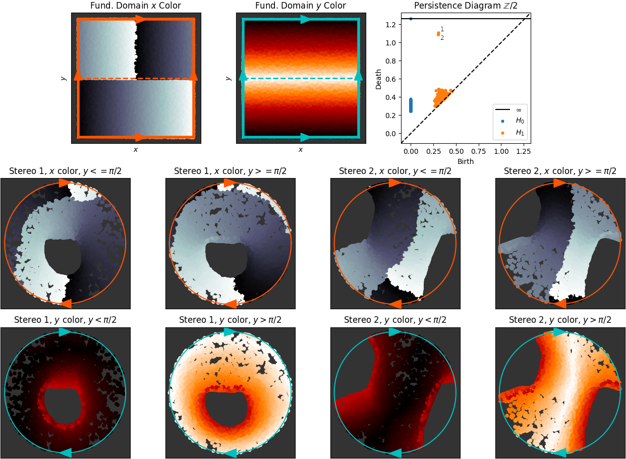
In fact, this is a 2 to 1 map, as shown in Figure 2. Just as a torus can be obtained from gluing two annuli together at their boundary, the Klein bottle can be obtained by gluing two Möbius strips at their boundary. Each one of these Möbius strips is visible in the odd and even columns of the bottom two rows of Figure 2, respectively. In particular, the loops and are at the center of each Möbius strip, and the boundaries of each Möbius strip at get identified at the center of the projective coordinates plot. We will observe similar projective coordinates for the sliding window of our Klein bottle time series in Section 5.2.
2.4.2 Circular Coordinates
The idea of using the bijection to construct circle-valued functions for data, from persistent cohomology classes, was first introduced by de Silva et. al. [8]. Their construction has shortcomings (not sparse, not transductive) which are addressed in [29]; the latter is the procedure we use in the paper and the one we describe next.
Let be a prime so that the homomorphism
induced by the projection , is surjective. Hence, any has a lift . Moreover, if is the inclusion homomorphism, then there are cochains and so that is the unique harmonic cocycle representative of and . From this data we define
where
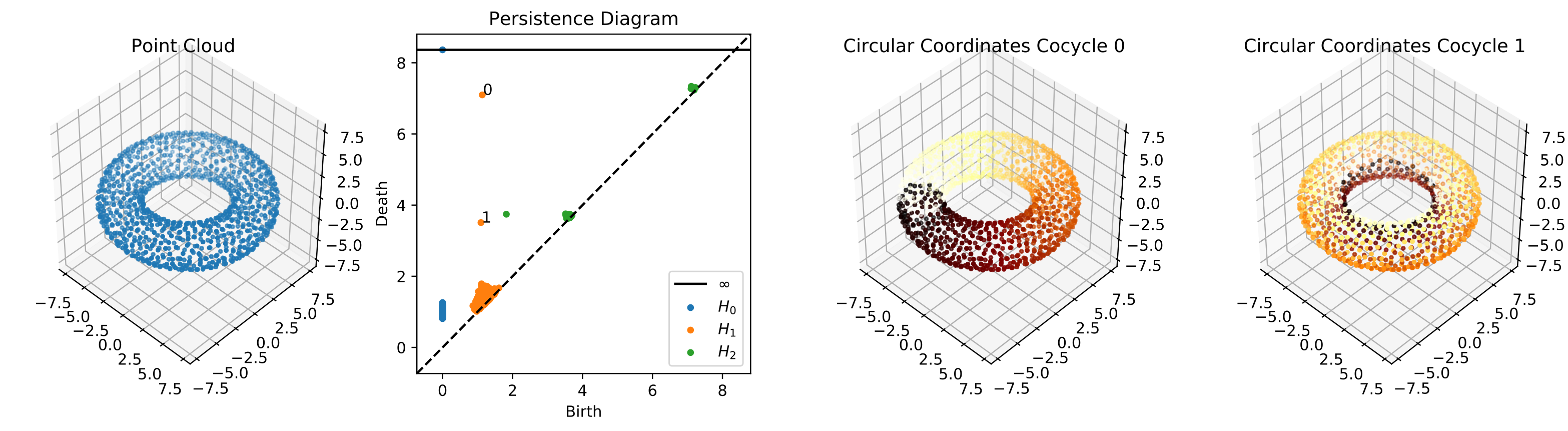
Figure 3 shows an example of this algorithm on a point cloud sampled from a torus, using 400 landmarks. In this example, the algorithm is able to find maps from the points to the inner and outer circle of the torus.
3 Preliminary Examples: Distance To A Point As Observation Function
To motivate a more general development of good observation functions on manifolds, we first explore a very specific genre of observation functions: those which arise as the distance to a specified point in the manifold. We then verify the geometric integrity of a delay coordinate mapping of the resulting time series using persistent homology and Eilenberg-Maclane coordinates on a few examples. Through these tools and a visual comparison of the time series to known examples, we will already be able to explain quite a lot, including motivating both conditions of Theorem 4.1, though a full development of the theory in Section 4 is needed to justify these choices of observation functions.
In the discussion below, all of our observation functions are of the form , where is some metric chosen on the manifold and is some fixed point on the manifold which is our “reference distance point.”
Example 3.1.
Flat torus

We first examine the planar torus , parameterized by . As our dynamics, we take the irrational winding , and the observation is the flat geodesic distance between and the point . This is shown in Figure 4. After performing a delay embedding on the resulting time series with window length of 30 samples, we see two persistent classes and 1 persistent class, which is the signature of a torus. Furthermore, circular coordinates resulting from the top two persistent classes in recovered the full original flow specification.
Example 3.2.
Flat Klein Bottle

As in our projective coordinates example in Figure 2, we now form a quotient on the domain of the flat torus to create a Klein bottle, via the automorphism . Then, the metric on the torus descends to the Klein bottle via . We use a slightly modified weighted flat metric as our distance measure for the observation function; that is
| (3) |
In this particular example, we let and , and we take an observation to the point ; that is, . Finally, we use a flow with a very shallow slope, , in the fundamental domain . After performing a sliding window embedding with a window length of 30 samples, we see two persistent classes in and one persistent class in with coefficients, but we only see one class in and no classes in with coefficients. This is indeed the signature of a Klein bottle. We will show projective coordinates on a similar example with a slightly different observation function in Section 5.2, and we will explain more intuitively visual features of the time series at that point.
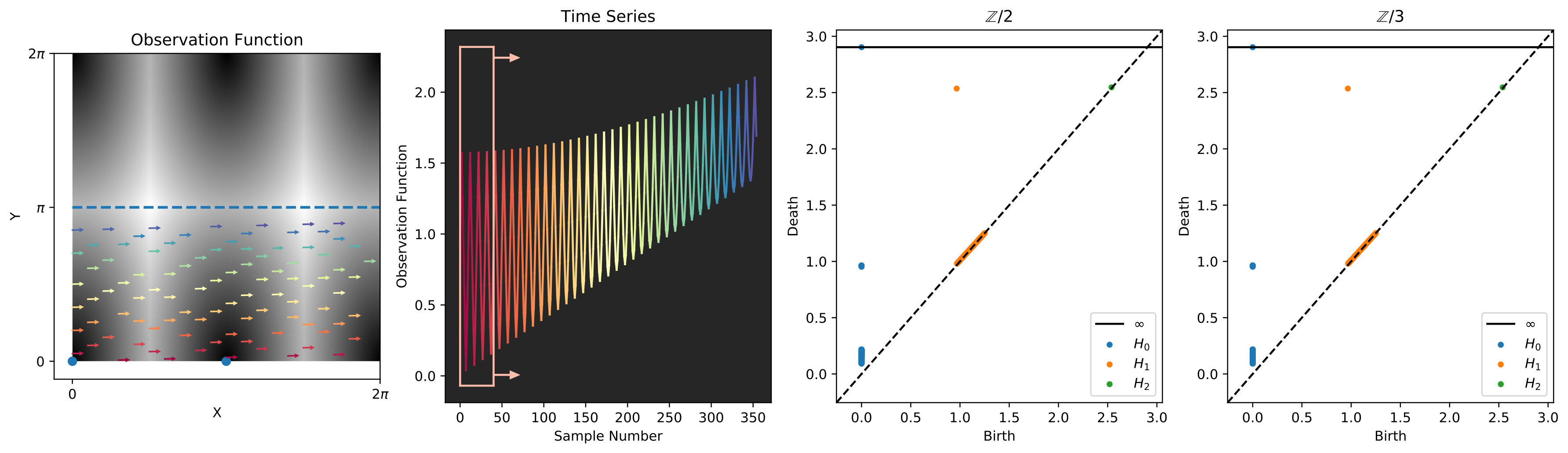
Note that not every distance function will lead to a reconstruction of the Klein bottle. For instance, if we use the same flow but an observation function , as in Figure 6, then the sliding window embedding of the resulting time series degenerates to a cylinder, because there exist pairs of points with the same observation curves under the flow. This motivates condition 2 in Theorem 4.1.
Example 3.3.
Sphere

We now reconstruct the sphere from a given trajectory and distance function. Tralie [38] showed empirically that a sliding window embedding of a helical trajectory, under the observation function on the sphere which is the arclength from some point on the sphere, yields an embedding of the sphere. We replicate this here. More specifically, we parameterize the unit sphere in spherical coordinates (where is azimuth and is elevation from the north pole), we let , and the let the observation to a point be
| (4) |
We repeat this here in Figure 7. In this example, simple linear dimension reduction via PCA is able to recover the most of the geometry of the sliding window point cloud, though spherical coordinates are also possible in the Eilenberg-MacLane framework [28].
One pitfall in this example is that the observation point cannot lie on the equator or the north or south poles; that is, . In these cases, the helix structure is flattened to a spiral,so the sliding window embedding degenerates to a disc. This motivates the “derivative rank” condition, or condition 1 in Theorem 4.1.
Example 3.4.
Projective plane

We can extend the scheme that we used in Example 3.3 to the projective plane by taking a flow only on the upper hemisphere and performing the antipodal identification at the equator . The flow is the same, but the observation function changes to
| (5) |
Figure 8 shows this result, in which a single highly persistent point is present for both and using coefficients, but in which none are present for , which is a correct signature of . Interestingly, the quotient identification is visible in the time series itself; the time series in Figure 8 can be obtained from the time series in Figure 7 by reflecting values above the line across that line. This is because the maximum distance between any two points on is . Additionally, both the sphere time series and the Möbius loop time series () are visible in Figure 8. The time series starts off in a spiral, which fills out a disc, and this disc transitions to a spiraling Möbius loop time series which fills out the strip. This visually reflects the fact that is the connected sum of a disc and the boundary of a cross-cap. We will use a similar intuition to explain the Klein bottle time series in Section 5.2.
Example 3.5.
Genus 2 surface

Finally, we show a time series whose sliding window embedding lies on the two holed torus. We use an irrational flow with slope , with an observation function as the squared flat metric on the fundamental domain [42] represented by an octagon with opposite sides identified. Figure 9 shows the result, in which four highly persistent dots are visible in and a single persistent dot is visible in , matching what is expected of the homology of a genus 2 surface.
4 Main Theorem: Characterizing Good Observation Functions
As our main theoretical contribution, we now state more general conditions for good observation functions. Let be a compact manifold of dimension , a smooth function, and a vector field with flow . Applying to an integral curve through a point yields a real-valued function
in , the observation curve of . For sufficiently nice and , one can recover the point from a finite uniform sampling of . More precisely, the Takens map defined by
is an embedding for some dimension and flow time . For such and we say is a good observation for .
4.1 Motivation for the approach
As a simple example, take , , and . The point is uniquely determined by sampling the two values and and the Takens map
is an embedding, so is a good observation.
On the other hand, the doubly periodic function is not a good observation function. Indeed, any integral curve is invariant under a -shift of , as cannot distinguish between any flow of and . In fact, the good observation functions on for the rotational dynamic are precisely ones with minimum period
In higher dimensions the task of recovering from becomes less clear. Consider the torus and given by
and an irrational flow
and thus for we have the observation curve
For to be good, there must be a such that each is uniquely determined by sampling along the integral curve at finitely many -steps. Since we are free to shrink and increase , it is natural to examine infinitesimal changes of along the flow . The derivatives
up to 3rd order yield the linear equation
Equivalently, over , the linear system
has invertible Vandermonde matrix and one can solve for and . Therefore is uniquely determined by ’s. Choosing small enough so that is close to the 3rd order Taylor polynomial of about , we see that is uniquely determined (modulo ) by a -uniform finite sampling of .
4.2 Main theorem and proof
The above calculation illustrates our approach to determining whether is good: by studying the Taylor coefficients . Note that is the -fold derivation of applied to at , i.e., in Lie derivative notation,
is the linear operator on tensor fields which measures infinitesimal change along , i.e. if is a tensor then
Writing for the differential of , and for exterior product, we now state the main result:
Theorem 4.1.
The Takens map is an embedding for some and flow time , if the following conditions hold:
- 1.
For any point of there is an -tuple of nonnegative integers such that the -form
is nonzero at some point on the integral curve .
- 2.
For any pair of distinct points the observation curves and are not identical.
Proof.
For to be an immersion, the cotangent vectors
must span an -dimensional space for all . Equivalently, for any point there must be a strictly increasing -tuple of indices such that the determinant -form does not vanish at , i.e.
We require that be strictly increasing because a wedge product containing identical factors is zero.
The idea is to perform a convolution of the Taylor series of the cotangent curves and to use condition 1 above to choose sufficiently small so that for some . By compactness of , one makes a uniform choice of small so that is immersive and each observation curve is distinguished on some integer multiple of , thereby making injective.
Let be a time parameter for such that
is nonzero at . Write and for the set of all strictly increasing -tuples with degree
satisfying
Fix to be the minimal integer for which is nonempty (possible by condition 1 above).
Let be the by matrix with th entry
and the linear map given by in the th coordinate,
So the th component of the composition , viewed as an -tuple of -dependent cotangent vectors, yields the th order Taylor polynomial about of the cotangent curve :
By Cauchy-Binet formula applied to and , the top exterior product
has th order Taylor series expansion about with th coefficient
where
- •
is a nonzero constant depending only on
- •
and
is the nonzero determinant of the Vandermonde matrix with th entry
where we take .
By the minimality assumption on , all the lower degree Taylor coefficients, which contain for -tuples with degree strictly less than ,
are zero. So the Taylor expansion of has the form
where is the th order Taylor error term with vanishing limit
For for suitable choice of , there will be a dominating term in the sum over such that is nonzero. For the colexigraphically maximal element of , let be the maximal index such that , for all . Choose by making all terms right of large, so that
for all
So the th Taylor coefficient
is nonzero. Hence we may choose a time sufficiently close to so that the Taylor error is small and the inequality
holds for all in a neighborhood of , and this property remains invariant under shrinking closer to . By compactness of there is a finite collection of triples such that the collection of -forms
do not all vanish at any given point of and the cotangent vectors
specified by are linearly independent. Choose small enough so that there is an integer multiple of lying in the interval for each . Then the Takens map is an immersion for all bounding and .
So is locally injective and the difference map
does not vanish for all in an open neighborhood of the diagonal in , and this property is invariant under scaling and for an integer (with fixed).
For distinct , we may shrink so that and are distinguished on some integer multiple of and . By compactness of , there is a uniform choice of and making injective, hence an embedding.
∎
Remark 4.2.
While one can provide a lower bound for the dimension needed to yield a Takens embedding, the formula depends in a complicated way on and . In practice, choosing sufficiently large and small amounts to a dense sampling of a discrete time series.
5 An Application to Surfaces via Fourier theory
Now that we have our theory in hand, we can examine another class of observation functions which are constructed from Fourier modes, in addition to our distance-based observation functions in Section 3.
5.1 The Torus
We start by characterizing all smooth observations for a vector field of irrational flow
yielding toroidal delay embedding. For write the Fourier expansion
where is the th Fourier coefficient of . Set
the support of .
Theorem 5.1.
A smooth function is a good observation for an irrational winding if and only if the support of the Fourier coefficients generates as an abelian group.
Proof.
Write for the Fourier basis element. The -fold Lie derivative has Fourier coefficient
and thus Fourier expansion
Since is irrational, the coefficients
are nonvanishing and pairwise distinct. Therefore the Vandermonde matrix with entry
is nonsingular and the projection
can be written as an infinite sum
| (6) |
Hence the values of on a point uniquely determine
If generates , then there is some finite product
and thus , and similarly , are uniquely determined modulo by the observation curve and condition 2 of Theorem 4.1 above is satisfied.
If vanishes at for all , then by equation 6 above, the -form
also vanishes at for all pairs . Thus
and cannot generate . So condition 1 of Theorem 4.1 is satisfied if generates .
Conversely, suppose does not generate . By the classification of finitely generated abelian groups, there is a -basis
for such that is generated by
where and are integers not both . Then there is some such that
takes values in , so that for all . So for any point , is a distinct point with the same observation curve, and no Takens map can distinguish between and . ∎
Remark 5.2.
Theorem 5.1 can be strengthened to include rational windings. In this case one cannot expect the delay mapping to recover all Fourier modes of an observation function, but only those which are coprime to the slope of the winding.
Remark 5.3.
For the irrational winding on the torus, the Koopman eigenfunctions are given by the Fourier basis. The Vandermonde inversion in equation (6) above shows that the Fourier modes of an observation are determined by its delay mapping. We are not aware of such a connection between Takens and Koopman, though it seems natural in this context.
By Theorem 5.1, whether or not is good for an irrational flow depends only on the support . The quasiperiodic function
| (7) |
is the observation of along the irrational flow on the planar torus . A point cloud densely sampled from the sliding window coordinates given by 10 uniform shifts of yields a curve in with toroidal persistence.

5.2 The Klein bottle
As in our example in Section 2.4.1, we write the Klein bottle as the quotient of the torus by the automorphism . The irrational flow on the is not -invariant since is orientation reversing in the coordinate. To approximate the shallow flow in Figures 5 and 6 above, we construct a vector field which flows cyclically along a repellor and an attractor by restricting a linear flow to the fundamental domain and flatten it out on the boundary circles . For with irrational, let be a vector field on the rectangle given by
where is a smooth function on a neighborhood of with , making smooth. For example, . Then extends uniquely to a -invariant vector field on on , and therefore induces a vector field on .
Theorem 5.4.
Let be a -invariant function on . For fixed , the Takens map
induced by and for arbitrarily small and slope is an embedding if and only if the following conditions hold:
- 1.
and have period in and do not differ by a shift
- 2.
generates
Proof.
Suppose is good for . Since flows horizontally at , condition 1) must hold so that each point is uniquely determined by its observation curve. Condition 2) must hold as well, since is given by an irrational winding away from the -neighborhood of and the same argument as in Theorem 5.1 above applies for sufficiently shallow slope because is fixed.
Conversely, suppose conditions 1) and 2) hold. is given by an irrational flow away from the -neighborhood of . Furthermore, any point in the -strip with may be flowed to a point where has irrational slope. The same argument as in Theorem 5.1 shows that the Takens map restricts to an embedding on .
By condition 1, the observation curve of a point where uniquely determines modulo , and is periodic and therefore distinct from any observation curve for . So each point is uniquely determined by its observation curve as per condition 2) of Theorem 4.1.
It remains to show that the Takens map is immersive at . If not, then vanishes on the circles , a neighorhood about which would fail to immerse, a contradiction. ∎
According to Theorem 5.4, the “simplest” -symmetric good observation is
| (8) |
Indeed, the Fourier coefficients of are supported at , which generates . Along the limit cycles we have and , which are distinct and doubly periodic.
Intuitively, the term is responsible for delay-mapping the limit cycles via a double covering. Without this term, the boundary , along the bottom and top boundaries, respectively. Not only are these boundaries no longer identified, but they also each map to a single point, turning the Klein bottle into a sphere. The delay mapping of fills two Möbius strips in conjuction with , while the term serves to “separate” the Möbius strips, as shown in the right hand side of Figure 12.
We can also see this by parameterizing the flow by a single variable and examining the time series directly. In this case, the time series is
| (9) |
for . Over small ranges of , the sine terms are approximately constant. The time series is then of the form ; that is, its sliding window embedding locally parameterizes the boundary of a Möbius strip [32]. As it moves further along, changes, and so it fills out the strip.

. Indeed the good observation function reproduces , as evidenced by the persistence diagram.

6 Discussion
It is clear what circular and toroidal observations look like in the time domain, and as we have mentioned, there are many applications that take advantage of this knowledge. The theory developed in this paper has enabled us to move beyond this and to develop examples of signals recovering other manifolds.
Also, by showing the existence of time series whose “attractors” are on twisted spaces, we also provide further motivation for TDA time series users to move beyond exclusively using in TDA. The latter is the default option across most applications of TDA in time series analysis, but it is possible that these pipelines are blind to important features, as some of our examples show.
Moreover, just as circular and toroidal sliding window embeddings have interpretations in terms of physical phenomena, the presence of Klein bottles, Moebius strips, spheres, projective planes, etc, should also have practical meaning. It is unlikely that one could recognize the significance of these time series in the wild without such examples in hand, and being primed as such makes it more likely that we will be able to discover physical examples where non-orientable state spaces are natural.
Finally, we note that not only do we have a method for producing time series recovering other manifolds, which we have validated empirically using persistent homology and Eilenberg MacClane coordinates, but the method is backed by a theorem that indicates exactly when it will succeed/fail.
References
- [1] Hassan Arbabi. Introduction to koopman operatory theory of dynamical systems. 2018.
- [2] Ulrich Bauer. Ripser: a lean c++ code for the computation of vietoris-rips persistence barcodes. Software available at https://github. com/Ripser/ripser, 2017.
- [3] Juan P Bello. Measuring structural similarity in music. IEEE Transactions on Audio, Speech, and Language Processing, 19(7):2013–2025, 2011.
- [4] Elodie F Briefer, Anne-Laure Maigrot, Roi Mandel, Sabrina Briefer Freymond, Iris Bachmann, and Edna Hillmann. Segregation of information about emotional arousal and valence in horse whinnies. Scientific reports, 4:9989, 2015.
- [5] Gunnar Carlsson. Topology and data. Bulletin of the American Mathematical Society, 46(2):255–308, 2009.
- [6] William Crawley-Boevey. Decomposition of pointwise finite-dimensional persistence modules. Journal of Algebra and its Applications, 14(05):1550066, 2015.
- [7] Suddhasattwa Das and Dimitrios Giannakis. Delay-coordinate maps and the spectra of koopman operators. arXiv preprint arXiv:1706.08544, 2017.
- [8] Vin De Silva, Dmitriy Morozov, and Mikael Vejdemo-Johansson. Persistent cohomology and circular coordinates. Discrete & Computational Geometry, 45(4):737–759, 2011.
- [9] Vin de Silva, Primoz Skraba, and Mikael Vejdemo-Johansson. Topological analysis of recurrent systems. In Workshop on Algebraic Topology and Machine Learning, NIPS, 2012.
- [10] Herbert Edelsbrunner and John Harer. Persistent homology-a survey. Contemporary mathematics, 453:257–282, 2008.
- [11] Herbert Edelsbrunner and John Harer. Computational topology: an introduction. American Mathematical Soc., 2010.
- [12] Herbert Edelsbrunner and Ernst P Mücke. Three-dimensional alpha shapes. ACM Transactions on Graphics (TOG), 13(1):43–72, 1994.
- [13] Saba Emrani, Harish Chintakunta, and Hamid Krim. Real time detection of harmonic structure: A case for topological signal analysis. In Acoustics, Speech and Signal Processing (ICASSP), 2014 IEEE International Conference on, pages 3445–3449. IEEE, 2014.
- [14] Jordan Frank, Shie Mannor, and Doina Precup. Activity and gait recognition with time-delay embeddings. In AAAI. Citeseer, 2010.
- [15] Hitesh Gakhar and Jose A Perea. Sliding window persistence of quasiperiodic functions. 2018.
- [16] Robert W Ghrist. Elementary applied topology. Createspace, 2014.
- [17] Bryan Glaz, Igor Mezić, Maria Fonoberova, and Sophie Loire. Quasi-periodic intermittency in oscillating cylinder flow. Journal of Fluid Mechanics, 828:680–707, 2017.
- [18] Allen Hatcher. Algebraic Topology. Cambridge University Press, 2002.
- [19] Hanspeter Herzel, David Berry, Ingo R Titze, and Marwa Saleh. Analysis of vocal disorders with methods from nonlinear dynamics. Journal of Speech, Language, and Hearing Research, 37(5):1008–1019, 1994.
- [20] Holger Kantz and Thomas Schreiber. Nonlinear time series analysis, volume 7. Cambridge university press, 2004.
- [21] Firas A Khasawneh and Elizabeth Munch. Chatter detection in turning using persistent homology. Mechanical Systems and Signal Processing, 70:527–541, 2016.
- [22] B. O. Koopman. Hamiltonian systems and transformation in hilbert space. Proceedings of the National Academy of Sciences, 17(5):315–318, 1931.
- [23] Igor Mezić. Analysis of fluid flows via spectral properties of the koopman operator.
- [24] Katherine Morrison, Anda Degeratu, Vladimir Itskov, and Carina Curto. Diversity of emergent dynamics in competitive threshold-linear networks: a preliminary report. arXiv preprint arXiv:1605.04463, 2016.
- [25] David D Nolte. The tangled tale of phase space. Physics today, 63(4):33–38, 2010.
- [26] Jose A Perea. Persistent homology of toroidal sliding window embeddings. In Acoustics, Speech and Signal Processing (ICASSP), 2016 IEEE International Conference on, pages 6435–6439. IEEE, 2016.
- [27] Jose A Perea. A brief history of persistence. arXiv preprint arXiv:1809.03624, 2018.
- [28] Jose A Perea. Multiscale projective coordinates via persistent cohomology of sparse filtrations. Discrete & Computational Geometry, 59(1):175–225, 2018.
- [29] Jose A Perea. Sparse circular coordinates via principal -bundles. arXiv preprint arXiv:1809.09269, 2018.
- [30] Jose A Perea. Topological time series analysis. Notices of the American Mathematical Society, 66(5), 2019.
- [31] Jose A Perea, Anastasia Deckard, Steve B Haase, and John Harer. Sw1pers: Sliding windows and 1-persistence scoring; discovering periodicity in gene expression time series data. BMC bioinformatics, 16(1):257, 2015.
- [32] Jose A Perea and John Harer. Sliding windows and persistence: An application of topological methods to signal analysis. Foundations of Computational Mathematics, 15(3):799–838, 2015.
- [33] Emil Plesnik, Olga Malgina, Jurij F Tasic, Saso Tomazic, and Matej Zajc. Detection and delineation of the electrocardiogram qrs-complexes from phase portraits. 2014.
- [34] Joan Serra, Xavier Serra, and Ralph G Andrzejak. Cross recurrence quantification for cover song identification. New Journal of Physics, 11(9):093017, 2009.
- [35] Cornelis J Stam. Nonlinear dynamical analysis of eeg and meg: review of an emerging field. Clinical Neurophysiology, 116(10):2266–2301, 2005.
- [36] Floris Takens et al. Detecting strange attractors in turbulence. Lecture notes in mathematics, 898(1):366–381, 1981.
- [37] Christopher Tralie, Nathaniel Saul, and Rann Barr-On. Ripser.py: A lean persistent homology library for python. Journal of Open Source Software (JOSS), 2018.
- [38] Christopher J Tralie. Geometric Multimedia Time Series. Duke ph.d. dissertation, Department of Electrical and Computer Engineering, Duke University, 2017.
- [39] Christopher J Tralie and John Harer. Moebius beats: The twisted spaces of sliding window audio novelty functions with rhythmic subdivisions. In 18th International Society for Music Information Retrieval (ISMIR), Late Breaking Session, 2017.
- [40] Christopher J. Tralie and Jose A. Perea. (quasi)periodicity quantification in video data, using topology. SIAM Journal on Imaging Sciences, 11(2):1049–1077, 2018.
- [41] Vinay Venkataraman, Karthikeyan Natesan Ramamurthy, and Pavan Turaga. Persistent homology of attractors for action recognition. In Image Processing (ICIP), 2016 IEEE International Conference on, pages 4150–4154. IEEE, 2016.
- [42] Anton Zorich. Flat surfaces. Frontiers in number theory, physics, and geometry I, pages 439–585, 2006.