Singlet $s^{\pm}$-wave pairing in quasi-one-dimensional ACr₃As₃ (A=K, Rb, Cs) superconductors

The crystal structure of KCr₃As₃ and its sister compounds is shown in Fig.1 (a), which belongs to the space group $P6_{3}/m$ (point group $C_{6h}$). Their basic building blocks are 1D chains of double-walled subnanotubes of [Cr₃As₃]_∞. The Cr₃As₃ units stack in alternating fashion along the chain direction, such that each unit cell contains two sublayers, A and B. The chains are separated by the alkali cations.

The band structure of KCr₃As₃ was predicted by using DFT as implemented in the Vienna ab initio simulation pack (VASP) [23, 24]. We employed the generalized gradient approximation (GGA) in the form of Perdew-Burke-Ernzerhof (PBE) [25] to describe the exchange-correlation effects. The electron-ion interactions was simulated using projector-augmented-wave (PAW) potentials with the energy cutoff of 500 eV[26]. Charge density calculations were performed on $8\times 8\times 12$ Monkhorst-Pack sampling in the Brillouin zone.

The band structure thus obtained is shown in Fig.1 (b). One can clearly see that the five bands (marked as $\alpha,\beta,\gamma,\delta,\varepsilon$) crossing with the Fermi level are dominated by the 3d${}_{z^{2}}$, the 3d${}_{x^{2}-y^{2}}$ and the 3d_xy orbitals of Cr atoms. Overall, these orbitals are mixed together but the relative contributions to the metallic bands are different. The 3d${}_{x^{2}-y^{2}}$ and the 3d_xy orbitals mix and mainly contribute to the two 3D FSs (which belong to the $\alpha$- and $\beta$- bands) and the two quasi-1D FSs (which belong to the $\delta$- and $\gamma$- bands), while the 3d${}_{z^{2}}$ orbital is relative decoupled and forms one quasi-1D FS (which belong to the $\varepsilon$- band). The five FSs are plotted in Fig.1 (c). The band structure and FS obtained here are consistent with those in a previous report[27].

To obtain an effective model, a sparse $4\times 4\times 6$ $\Gamma$-centered sampling is utilized for establishing Wannier orbitals of virtual atoms localized at the center of each Cr triangle via WANNIER90 package[28], with the initial guess of d${}_{z^{2}}$ ($A^{\prime}$ representation) and (d${}_{x^{2}-y^{2}}$, d_xy) ($E^{\prime}$ representation) orbitals for unitary transformations. The structure of KCr₃As₃ can then be simplified to be chains of virtual atoms arranged in parallel, with each chain containing A and B sublattices. The obtained TB Hamiltonian in the momentum space can be expressed as

where $m,n=A,B$ label sublattices, $\sigma=\uparrow,\downarrow$ label spins and $\mu,\nu=1,2,3$ label orbitals $d_{z^{2}}$, $d_{xy}$ and $d_{x^{2}-y^{2}}$, respectively. Note that physically the orbital bases $d_{z^{2}}$, $d_{xy}$ and $d_{x^{2}-y^{2}}$ here are not the maximally localized Wannier wave functions around a real single Cr atom, but the superposition of the three atomic wave functions around the virtual center. Such Wannier wave functions can be dubbed as “molecular orbital”[11, 29], which are much more delocalized than conventional “atomic-orbital” Wannier bases localizing around a single atom[11, 29, 12, 13].

The minimum TB model which can capture all the qualitative aspects of the low energy part of the DFT band structure contains up to the next-nearest-neighbor hopping parameters in the $xy$-plane and the next-next-nearest-neighbor hopping parameters in the $z$-direction. The point-group symmetry allowed $h^{mn}_{\mu\nu}(\bm{k})$ thus obtained can be expressed as following,

and

Here $x=\frac{\sqrt{3}}{2}{k_{x}a_{0}}$, $y=\frac{1}{2}k_{y}a_{0}$ and $z=\frac{1}{2}k_{z}c_{0}$. The values of the above parameters are listed in the Appendix.

The TB model actually adopted in our following calculations is a more rigourous one expressed as,

with $\mu,\nu=1,\cdots,6$ indicating the orbital-sublattice indices. The elements of the $h(\bm{k})$ matrix is,

Here $\bm{a_{1}}=(\frac{\sqrt{3}}{2}a_{0},-\frac{1}{2}a_{0},0)$, $\bm{a_{2}}=(0,a_{0},0)$ and $\bm{a_{3}}=(0,0,c_{0})$. The data of $t^{r_{1},r_{2},r_{3}}_{\mu\nu}$ for $r_{1,2}\in[-2,2]$, $r_{3}\in[-4,4]$ and $\mu,\nu\in[1,6]$ is provided in the Supplementary Material [30]. The band structure thus obtained shown in the inset of Fig. 1(b) (red) is well consistent with that of the DFT (black) at low energy near the Fermi level.

Following the standard multi-orbital RPA approach [31, 32, 33, 34, 35, 36, 37, 38, 39, 40, 41], we first define the following bare susceptibility in the normal state for the non-interacting case:

Here $\langle\cdots\rangle_{0}$ denotes the thermal average for the noninteracting system, $T_{\tau}$ denotes the imaginary time-ordered product, and $p,q,s,t=1,\cdots,6$ are the orbital-sublattice indices. Fourier transformed to the imaginary frequency space, the bare susceptibility can be expressed by the following explicit formulism:

where $\alpha,\beta=1,\cdots,6$ are band indices, $\varepsilon^{\alpha}_{\bm{k}}$ and $\xi^{\alpha}\left(\bm{k}\right)$ are the $\alpha$-th eigenvalue (relative to the chemical potential $\mu_{c}$) and eigenvector of the TB model, respectively, and $n_{F}$ is the Fermi-Dirac distribution function.

In Fig. 2, we show the $\bm{k}$-dependence of the largest eigenvalue of the susceptibility matrix $\chi^{(0)}_{pqst}(\bm{k},i\omega_{n}=0)$ along the high-symmetry lines in the Brillouin zone in (a), on the $k_{z}=0$ plane in (b) and on the $k_{z}=\pi$ plane in (c). Clearly, the largest eigenvalue peaks near the A-point $(0,0,\pi)$ and the M-points $(0,\pi,0),(\pi,0,0),(\pi,\pi,0)$. Detailed inspection reveals that the susceptibility peak near the A-point originates mainly from the nesting between the top and bottom surfaces of the 1D $\gamma,\delta$ FSs while that near the M-points originates from the nesting between different side surfaces of the 3D $\alpha,\beta$ FSs. The nearly equal peak values between the A- and M- points suggest competing wave vectors at these momenta for the density wave orders emerging at sufficiently strong interactions. Besides, there are a few other peaks appearing in Fig. 2, including the one centering at $(0,0,0.83\pi)$ near the A-point, which originates mainly from the nesting between the top (bottom) surfaces of the 3D $\alpha,\beta$ FSs and the bottom (top) surfaces of the 1D $\gamma,\delta$ FSs. This peak is intimately related to the origin of the $s^{\pm}$-wave pairing obtained below.

We further define the spin $(s)$ and charge $(c)$ susceptibilities. At the RPA level, the renormalized spin and charge susceptibilities of the system read

Here the nonzero elements $U^{(s,c)\mu\nu}_{\theta\xi}$ of $U^{(s,c)}$ satisfy $\mu,\nu,\theta,\xi\leq 3$ or $>3$ simultaneously, which are as follow,

In Eq.(18), $\chi^{(s,c,0)}(\bm{k},i\omega_{n})$ and $U^{(s,c)}$ are operated as $6^{2}\times 6^{2}$ matrices (see for example in Ref[37]).

Generally, repulsive $U^{(s,c)}$ enhances $\chi^{(s)}$ and suppresses $\chi^{(c)}$. Increasing $U$ to some critical value $U_{c}$ (fixing $J_{H}/U$), $\chi^{(s)}(\bm{k},i\omega_{n}=0)$ will diverge first at the momentum ${\bm{k}=\bm{Q}=(0,0,\pi)}$, in close competition with the momenta ${\bm{k}=\bm{Q}=(\pi,0,0),(0,\pi,0)}$ and ${\bm{(}\pi,\pi,0)}$, suggesting the onset of SDW order with the corresponding wavevectors. Note that the SDW wavevectors $\bm{Q}$ in the KCr₃As₃ obtained here suggest inter-unit-cell SDW order, which stands in strong contrast with the inter-unit-cell ferromagnetic order with $\bm{Q}=(0,0,0)$ obtained for the A₂Cr₃As₃ family[12]. The RPA approach is only valid for $U<U_{c}$.

At $U<U_{c}$, Cooper pairing may develop through exchanging spin and/or charge fluctuations. In particular, we consider Cooper pair scatterings both within and between the bands, hence both intra- and inter-band effective interactions $V^{\alpha\beta}(\mathbf{k,k^{\prime}})$[12] (here $\alpha/\beta=1,\cdots,6$ are band indices) are accounted for. From the effective interaction vertex $V^{\alpha\beta}(\mathbf{k,k^{\prime}})$, we obtain the following linearized gap equation (23):

Here the integration runs along the $\beta$- FS, $v^{\beta}_{F}(\bm{k}^{\prime})$ is the corresponding Fermi velocity, and $\bm{k}^{\prime}_{\parallel}$ is the component of $\bm{k}^{\prime}$ along the FS. Superconducting pairing in various channels emerge as the eigenstates of the above gap equation. The leading pairing $\Delta_{\alpha}(\bm{k})$ is given by the eigenstate corresponding to the largest eigenvalue $\lambda$. The critical temperature $T_{c}$ is related to $\lambda$ through $T_{c}\propto e^{-1/\lambda}$.

The eigenvector(s) $\Delta_{\alpha}(\bm{k})$ for each eigenvalue $\lambda$ obtained from gap equation (23) as the basis function(s) forms an irreducible representation of the $C_{6h}$ point group. In the absence of SOC, ten possible pairing symmetries are possible candidates for the system, which include five singlet pairings and five triplet pairings, as listed in Table.1. For each triplet pairing, there are three degenerate components, i.e., $\uparrow\downarrow+\downarrow\uparrow$, $\uparrow\uparrow$, $\downarrow\downarrow$, and the degeneracy between them can be lifted by finite SOC.

The phase diagram as parameterized by the interactions $(U,J_{H}/U)$ is shown in Fig. 3(a). Roughly speaking, SDW is favored at $U>U_{c}$, which is around $0.2\sim 0.3$eV and is $J_{H}/U$-dependent in the present model. At weaker $U$, three superconducting phases appear, including spin-triplet $p_{z}$- and $f$-wave pairings and an $s$-wave pairing. The evolution of the different pairing channels are shown in Fig. 4(a) as a function of $J_{H}/U$ at a representative interaction strength $U=0.15$eV, and in Fig. 4(b) as a function of $U$ at a representative $J_{H}/U=0.2$. From the above results one finds: at weak $U$ the $f$-wave pairing becomes more favorable at sufficiently strong Hund’s rule coupling ($J_{H}/U>r_{c}\approx\frac{1}{3}$), while $p_{z}$-wave pairing develops for weaker Hund’s rule coupling; at intermediate $U$, the $s$-wave pairing dominates. For comparison, Fig. 3(b) shows the phase diagram obtained from a previous study of the 233-family[13].

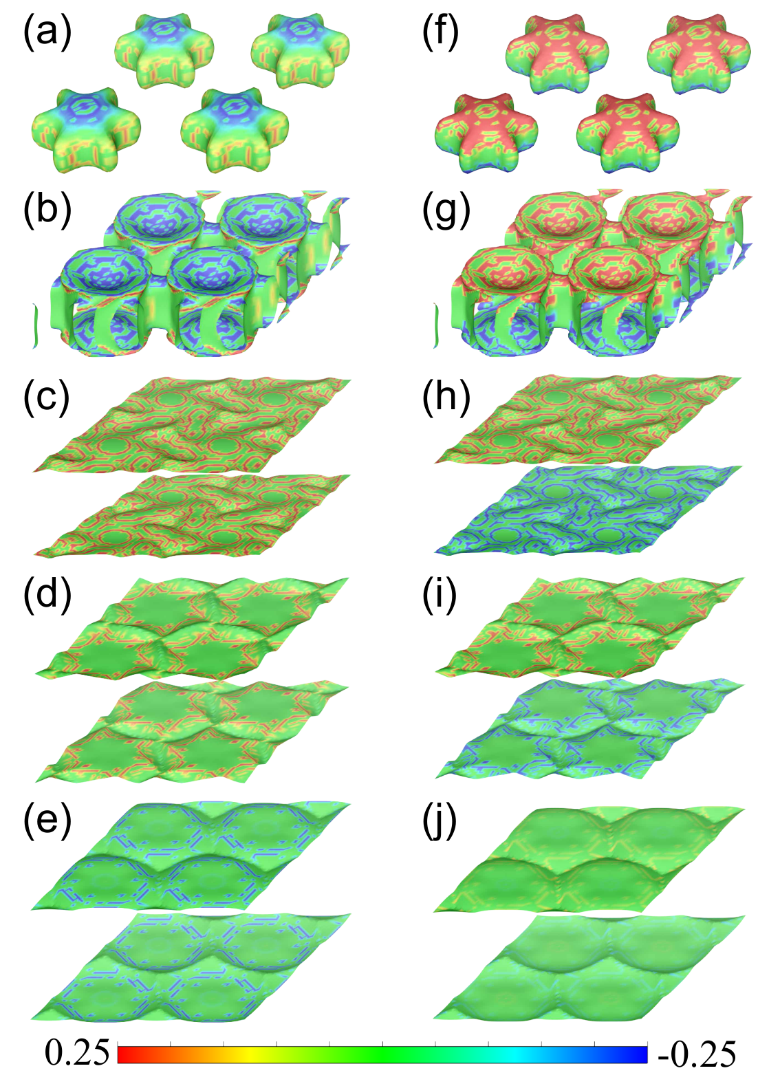
The most striking difference between Fig. 3(a) and (b) is the occurrence of $s$-wave pairing in the 133-family at intermediate values of $U$ and $J_{H}/U$. The normalized gap functions of the $s$-wave pairing on the five FSs are shown in Fig.5(a)-(e). The gap function is invariant under all $C_{6h}$ symmetry operations, and the gap amplitudes on all the five FSs are comparable. While the gap is positive on the two quasi-1D $\gamma$- and $\delta$-bands, it is negative on the quasi-1D $\varepsilon$-band. On the 3D $\alpha$- and $\beta$-bands, the gap function acquires opposite signs on the top/bottom and the side surfaces, giving rise to accidental nodal lines. The sign-changing character resembles the $s^{\pm}$-pairing proposed for iron-based SCs. In the present work, the $s^{\pm}$-pairing is driven by the SDW fluctuations and its sign structure is roughly consistent with the FS-nesting behavior as we discussed in association with Fig.2. To be more concrete, the nesting vector near ${\bm{Q}=(0,0,0.83\pi)}$ connects the top/bottom surfaces of the 3D $\alpha,\beta$ FSs and the bottom/top surfaces of the 1D $\gamma,\delta$ bands. As a result, the gap function on the corresponding nested portions of the FSs develops opposite signs.

The $p_{z}$-wave pairing for weak $U$ and $J_{H}/U$ shown in Fig. 3(a) in the 133 family is similar to that in the 233 family[12, 13] shown in Fig. 3(b). Although the Cooper pairing in the weak $U$ and $J_{H}/U$ limit is still driven by spin fluctuations, the pairing symmetry obtained can be markedly different from that at intermediate $U$, because in this limit the bare interaction dominates the effective interaction. Although the dominant bare interaction in the weak $U$ limit will suppress any pairing symmetry, the $s$-wave will be most suppressed due to the following reason. The gap function of an $s$-wave (either $s^{++}$ or $s^{\pm}$) pairing have a nonzero average value over the entire Brilloui zone. As a result, when Fourier-transformed back into the real space, the $s$-wave pairing will inevitably possess a nonzero on-site pairing component, which is unfavored by the dominant repulsive on-site bare interaction in the weak $U$ limit with $J_{H}/U<r_{c}$. Hence, in the weak-$U$ limit with $J_{H}/U<r_{c}$, non-s-wave pairing is generally more favorable, and in the present study, the $p_{z}$-wave emerges as the leading pairing instability. Fig. 5(f)-(j) show the normalized gap function in this channel. This pairing is invariant under a $C_{6}$ rotation, but changes sign under a mirror reflection about the $xy$ plane. As a result, line nodes exist in the $xy$ plane on the 3D bands. Note that the pairing amplitude is much weaker on the $\varepsilon$-band than the other bands, presumably due to a relatively weak interband interaction involving the $\varepsilon$-band.

For $J_{H}/U>r_{c}$, the $f$-wave pairing in the 133 and 233-families also share the same origin: the orbitals become unstable to Cooper pairing at the bare level of the on-site Hubbard interactions. This pairing possesses a significant on-site pairing component. This pairing is even about the $k_{z}=0$ mirror plane, but changes sign under $C_{6}$ rotations. Therefore it also possesses line nodes.

The three degenerate components of the triplet $p_{z}$- and $f$-wave pairings are split once spin-rotational invariance is broken by SOC. In the present system, to leading order the symmetry-allowed SOC takes the following form,

where 2, 3 stand for the orbital indices, and we take $\lambda_{SOC}=10$meV. Classified according to the $S_{z}$ quantum number of Cooper pairing, possible pairing components include the $S_{z}=0$, i.e., $\uparrow\downarrow+\downarrow\uparrow$ component, and the $S_{z}=\pm 1$, i.e., $\uparrow\uparrow$ and $\uparrow\uparrow$ component. The $J_{H}/U$ dependence of the largest pairing eigenvalues $\lambda$ of the $S_{z}=0$ and $S_{z}=\pm 1$ components of the $p_{z}$- and the $f$-wave pairings obtained from RPA is shown in Fig. 6 with fixed $U=0.05$eV. Clearly, for the $p_{z}$-wave, the $S_{z}=0$ component wins over the $S_{z}=\pm 1$ one for any $J_{H}/U$. As for the $f$-wave, the $S_{z}=0$ component wins over the $S_{z}=\pm 1$ one only for small $J_{H}/U$, and the contrary is true for large $J_{H}/U$.

The $s$-wave SC predicted here in the KCr₃As₃ can be distinguished from the $p_{z}$-wave predicted in the K₂Cr₃As₃ by the following dc SQUID device as shown in Fig.7(a), where a loop of a conventional s-wave superconductor is coupled to the two ends of superconducting KCr₃As₃ or K₂Cr₃As₃ along the $z$ direction through superconductor-normal metal-superconductor (SNS) Josephson junctions. An externally applied magnetic flux $\Phi$ threads this loop. Due to the interference between the two branches of Josephson supercurrent, the maximum supercurrent (the critical current) $I_{c}$ in the circuit modulates with $\Phi$ according to

Here $I_{0}$ is the critical current of one Josephson junction, $\Phi_{0}=h/2e$ is the flux quantum. The phase shift $\delta\phi$ depends on the pairing symmetry. It is zero for an s-wave pairing and $\pi$ for $p_{z}$-wave. The different patterns of $I_{c}-\Phi$ relation can then be used to distinguish the two superconducting states, as demonstrated in Fig. 7.

The above Josephson interferometry is oblivious to the sign-changing character of the $s$-wave pairing. However, there exists another distinguishing feature of the $s^{\pm}$-wave pairing – the in-gap spin resonance mode in the superconducting state. The corresponding resonance peak emerges in the imaginary part of the dynamic spin susceptibility. Such a quantity can be easily obtained in the present RPA formalism.

Let’s define the following bare susceptibility in the superconducting state,

where $\langle\cdots\rangle_{sc,0}$ denotes the thermal average in the BCS mean-field state. In $\sigma^{i}_{\alpha\beta}$, $\alpha,\beta$ denote spin indices and $\sigma^{i}$ represents the $i$-th component of the Pauli matrix. In the spin-singlet pairing state, the spin SU(2) symmetry requires $\chi^{(sc,0)ij}_{pqst}(\bm{q},\tau)=\delta_{ij}\chi^{(sc,0)ii}_{pqst}(\bm{q},\tau)$, which allows us to only calculate $\chi^{(sc,0)+-}_{pqst}(\bm{q},\tau)$ and obtain $\chi^{(sc,0)zz}_{pqst}(\bm{q},\tau)=\frac{1}{2}\chi^{(sc,0)+-}_{pqst}(\bm{q},\tau)$.

The above bare susceptibility function $\chi^{(sc,0)+-}_{pqst}(\bm{q},\tau)$ is first Fourier transformed to the imaginary frequency space and then analytically continued to the real frequency axis via $i\omega_{n}\to\omega+i0^{+}$, after which we obtain the following retarded bare susceptibility:

with

and

Here the pairing gap $\Delta^{\alpha}_{\bm{k}}$ is a product of the dimensionless normalized gap function $\Delta_{\alpha}(\bm{k})$ solved in Eq.(23) and a global amplitude $\Delta_{0}$, i.e. $\Delta^{\alpha}_{\bm{k}}=\Delta_{0}\Delta_{\alpha}(\bm{k})$ ($|\Delta_{\alpha}(\bm{k})|_{\text{max}}=1$). Here, we take $\Delta_{0}=2$meV on account of the experimental superconducting $T_{c}\approx 5$ K.

The RPA susceptibility in the superconducting state is still defined by Eq.(18), but with $\chi^{(0)}(\bm{k},i\omega_{n})$ replaced by $\chi^{(sc,0)+-}(\bm{k},\omega)$ in Eq.(27). The quantity related to the inelastic neutron scattering experiment is the imaginary part $\chi^{\prime\prime}_{\text{spin}}(\bm{q},\omega)$ of the dynamic spin susceptibility $\chi^{+-}_{\text{spin}}(\bm{q},\omega)\equiv\sum_{ps}\chi^{+-}_{ppss}(\bm{q},\omega)$. The obtained $\chi^{\prime\prime}_{\text{spin}}(\bm{q},\omega)\equiv\text{Im}\chi^{+-}_{\text{spin}}(\bm{q},\omega)$ at zero temperature is shown in Fig. 8 as a function of $\omega$ for a typical fixed momentum $\bm{q}=(0,0,0.83\pi)$ near the nesting vector, in comparison with the renormalized results obtained in the non-superconducting normal state. Fig. 8 shows a pronounced spin resonance peak below $w=2\Delta_{0}$ in the $s^{\pm}$-wave state, which is absent in the normal state. Physically, the presence of this collective spin mode not only confirms the sign-changing character of the $s^{\pm}$-wave pairing in the 133 family, but also indicates the magnetic origin of the Cooper pairing. This resonance mode can be easily detected in inelastic neutron scattering measurements.

A remarkable property of the quasi-1D $s^{\pm}$-SC obtained here lies in that, similar with the case of quasi-2D $s^{\pm}$-wave iron-based SC[43], it can be equipped to engineer 1D TRI TSC via proximity effects between the $s^{\pm}$-wave KCr₃As₃ superconductor and a semiconductor wire with large Rashba SOC. As shown in Fig. 9(a), the quasi-1D KCr₃As₃ superconductor (blue) is parallel aligned close to a semiconductor wire along the Cr-chain direction (marked as the $z$-axis direction). The semiconductor wire has large Rashba SOC $\lambda_{R}$ and similar lattice constant with KCr₃As₃. By proximity effect, the superconducting pairing in the KCr₃As₃ will be delivered to the Rashba wire. Due to the repulsive Hubbard-interactions in our model, the on-site pairing component $\Delta_{0}$ of the $s^{\pm}$-wave SC should be weak and the inter-site-pairing component will be dominant. For the quasi-1D KCr₃As₃ superconductor, the dominant inter-site-pairing component should be the pairing $\Delta_{1}$ between nearest-neighbor (NN) unit-cell along the Cr-chain. We assume such pairing component structure will be delivered to the 1D Rashba wire via proximity effect.

The Hamiltonian for the Rashba wire with SC acquired via proximity to KCr₃As₃ reads,

Here $t$ is the NN hopping coefficient, $\lambda_{R}$ is the coefficient of the Rashba SOC, $\mu_{c}$ is the chemical potential, $\Delta_{0}$ and $\Delta_{1}$ are the on-site and NN- pairing amplitudes respectively. After Fourier-transformed to the momentum space, the Hamiltonian can be written as

with $\psi_{k}=\left(c_{k\uparrow},c_{k\downarrow}\right)^{T}$, $h(k)=\left(-2t\cos k-\mu_{c}\right)I+2\lambda_{R}\sin k\sigma^{y}$ and $\Delta_{k}=i\sigma^{y}\Delta\left(k\right)$. Here $\Delta\left(k\right)=\Delta_{0}+2\Delta_{1}\cos k$ is the gap function. This Hamiltonian is TRI.

From the criterion of TRI TSC in 1D[44], we should calculate the following $Z_{2}$ FS topological invariant (FSTI),

where the summation index $s$ represents any Fermi point between $0$ and $\pi$, and the real number $\delta_{s}$ is defined as[44]

Here $\left|n_{s},k_{s}\right\rangle$ is the eigenvector of $h_{k}$, with $k_{s}$ and $n_{s}$ denoting the momentum and band index for the Fermi-point $s$, $\mathcal{T}=i\sigma^{y}$ is the time-reversal matrix[44], and $\Delta^{\dagger}_{k}=-i\sigma^{y}\Delta\left(k\right)$. As a result, we have,

For each $k$, the two eigenvalues $\varepsilon^{\pm}(k)$ of $h_{k}$ are solved as $\varepsilon^{\pm}(k)=-2t\cos k-\mu_{c}\pm 2\lambda_{R}\sin k$. For each $\mu_{c}$, we have two Fermi-points $k_{\pm}$ within $(0,\pi)$, satisfying $\varepsilon^{\pm}(k_{\pm})=0$ respectively, with $k_{+}<k_{-}$. Therefore, the FSTI defined in Eq.(32) is written as

from which the criterion of TRI TSC is that the signs of $\Delta(k_{\pm})$ are different, known as the negative pairing. Noticing that the node of the gap function $\Delta(k)=0$ within $(0,\pi)$ solved as $k_{0}=\arccos(-\Delta_{0}/2\Delta_{1})$ is unique, the situation of negative pairing requires $k_{+}<k_{0}<k_{-}$ as shown in Fig. 9(b). This condition leads to $\mu_{c}\in(\frac{t\Delta_{0}}{\Delta_{1}}-2\lambda_{R}\sqrt{1-\frac{\Delta^{2}_{0}}{4\Delta^{2}_{1}}},\frac{t\Delta_{0}}{\Delta_{1}}+2\lambda_{R}\sqrt{1-\frac{\Delta^{2}_{0}}{4\Delta^{2}_{1}})}$. Particularly, the width of the energy window of $\mu_{c}$ required by TRI TSC is $4\lambda_{R}\sqrt{1-\frac{\Delta^{2}_{0}}{4\Delta^{2}_{1}}}$, which is non-zero when $\left|\frac{\Delta_{1}}{\Delta_{0}}\right|>\frac{1}{2}$. Such condition can be easily satisfied.

References

- [1] J.-K. Bao,J.-Y. Liu, C.-W. Ma, Z.-H. Meng, Z.-T. Tang, Y.-L. Sun, H.-F. Zhai, H. Jiang, H. Bai, C.-M. Feng, Z.-A. Xu, and G.-H. Cao, Superconductivity in Quasi-One-Dimensional K2Cr3As3 with Significant Electron Correlations, Phys. Rev. X 5, 011013 (2015).
- [2] Z.-T. Tang, J.-K. Bao, Y. Liu, Y.-L. Sun, A. Ablimit, H.-F. Zhai, H. Jiang, C.-M. Feng, Z.-A. Xu, and G.-H. Cao, Unconventional Superconductivity in Quasi-One-Dimensional Rb2Cr3As3, Phys. Rev. B 91, 020506(R) (2015).
- [3] Z.-T. Tang, J.-K. Bao, Z. Wang, H. Bai, H. Jiang, Y. Liu, H.-F. Zhai, C.-M. Feng, Z.-A. Xu, G.-H. Cao, Superconductivity in Quasi-One-Dimensional Cs2Cr3As3 with Large Interchain Distance, Sci. China Mater. 58(1), 16 (2015).
- [4] Q.-G. Mu, B.-B. Ruan, B.-J. Pan, T. Liu, J. Yu, K. Zhao, G.-F. Chen, and Z.-A. Ren, Superconductivity at 5 K in Quasi-One-Dimensional Cr-Based KCr3As3 Single Crystals, Phys. Rev. B 96, 140504 (2017).
- [5] T. Liu, Q.-G. Mu, B.-J. Pan, J. Yu, B.-B. Ruan, K. Zhao, G.-F. Chen, Z.-A. Ren, Superconductivity at 7.3 K in the 133-Type Cr-Based RbCr3As3 Single Crystals, Europhys. Lett. 120, 27006 (2017).
- [6] Q.-G. Mu, B.-B. Ruan, B.-J. Pan, T. Liu, J. Yu, K. Zhao, G.-F. Chen, and Z.-A. Ren, Ion-Exchange Synthesis and Superconductivity at 8.6 K of Na2Cr3As3 with Quasi-One-Dimensional Crystal Structure, Phys. Rev. Materials 2, 034803 (2018).
- [7] Q.-G. Mu, B.-B. R., K. Zhao, B.-J. Pan, T. Liu, L. Shan, G.-F. Chen, Z.-A. Ren, Superconductivity at 10.4 K in a Novel Quasi-One-Dimensional Ternary Molybdenum Pnictide K2Mo3As3, Sci. Bull. 63, 952 (2018).
- [8] K. Zhao, Q.-G. Mu, T. Liu, B.-J. Pan, B.-B. Ruan, L. Shan, G.-F. Chen, Z.-A. Ren, Superconductivity in Novel Quasi-One-Dimensional Ternary Molybdenum Pnictides Rb2Mo3As3 and Cs2Mo3As3, arXiv:1805.11577.
- [9] H. Jiang, G. H. Cao, and C. Cao, Electronic Structure of Quasi-One-Dimensional Superconductor K2Cr3As3 from First-Principles Calculations, Sci. Rep. 5, 16054 (2015).
- [10] J. J. Miao, F. C. Zhang, and Y. Zhou, Instability of Three-Band Tomonaga-Luttinger Liquid: Renormalization Group Analysis and Possible Application to K2Cr3As3, Phys. Rev. B 94, 205129 (2016).
- [11] Y. Zhou, C. Cao, and F. C. Zhang, Theory for superconductivity in alkali chromium arsenides A2Cr3As3 (A=K,Rb,Cs), Sci. Bull. 62, 208 (2017).
- [12] X. X. Wu, F. Yang, C. C. Le, H. Fan, and J. P. Hu, Triplet -Wave Pairing in Quasi-One-Dimensional A2Cr3As3 Superconductors (A=K,Rb,Cs), Phys. Rev. B 92, 104511 (2015).
- [13] L.-D. Zhang, X. X. Wu, H. Fan, F. Yang, and J. P. Hu, Revisitation of Superconductivity in K2Cr3As3 Based on the Six-Band Model, Europhys. Lett. 113, 37003 (2016).
- [14] G. M. Pang, M. Smidman, W. B. Jiang, J. K. Bao, Z. F. Weng, Y. F. Wang, L. Jiao, J. L. Zhang, G. H. Cao, and H. Q. Yuan, Evidence for Nodal Superconductivity in Quasi-One-Dimensional K2Cr3As3, Phys. Rev. B 91, 220502 (2015).
- [15] F. F. Balakirev, T. Kong, M. Jaime, R. D. McDonald, C. H. Mielke, A. Gurevich, P. C. Canfield, and S. L. Bud’ko, Anisotropy Reversal of the Upper Critical Field at Low Temperatures and Spin-Locked Superconductivity in K2Cr3As3, Phys. Rev. B 91, 220505 (2015).
- [16] J. Yang, Z.-T. Tang, G.-H. Cao, and G.-Q. Zheng, Ferromagnetic Spin Fluctuation and Unconventional Superconductivity in Rb2Cr3As3 Revealed by 75As NMR and NQR, Phys. Rev. Lett. 115, 147002 (2015).
- [17] H.-Z. Zhi, T. Imai, F.-L. Ning, J.-K. Bao, and G.-H. Cao, NMR Investigation of the Quasi-One-Dimensional Superconductor K2Cr3As3, Phys. Rev. Lett. 114, 147004 (2015).
- [18] D. T. Adroja, A. Bhattacharyya, M. Telling, Yu. Feng, M. Smidman, B. Pan, J. Zhao, A. D. Hillier, F. L. Pratt, and A. M. Strydom, Superconducting Ground State of Quasi-One-Dimensional K2Cr3As3 Investigated Using SR Measurements, Phys. Rev. B 92, 134505 (2015).
- [19] D. T. Adroja, A. Bhattacharyya, M. Smidman, A. D. Hillier, Yu. Feng, B. Pan, J. Zhao, M. R. Lees, A. M. Strydom, P. K. Biswas, Nodal superconducting gap structure in the quasi-one-dimensional Cs2Cr3As3 investigated using SR measurements, J. Phys. Soc. Jpn. 86, 044710 (2017).
- [20] K. M. Taddei, Q. Zheng, A. S. Sefat, and C. de la Cruz, Coupling of Structure to Magnetic and Superconducting Orders in Quasi-One-Dimensional K2Cr3As3, Phys. Rev. B 96, 180506(R) (2017).
- [21] W. Kohn and J. M. Luttinger, New Mechanism for Superconductivity, Phys. Rev. Lett. 15, 524 (1965).
- [22] S. Raghu, S. A. Kivelson and D. J. Scalapino, Superconductivity in the Repulsive Hubbard Model: An Asymptotically Exact Weak-Coupling Solution, Phys. Rev. B 81, 224505 (2010).
- [23] G. Kresse and J. Furthmüller, Efficient Iterative Schemes for ab initio Total-Energy Calculations Using a Plane-Wave Basis Set, Phys. Rev. B 54, 11169 (1996).
- [24] G. Kresse and J. Hafner, Ab initio Molecular Dynamics for Open-Shell Transition Metals, Phys. Rev. B 48, 13115 (1993).
- [25] J. P. Perdew, K. Burke and M. Ernzerhof, Generalized Gradient Approximation Made Simple, Phys. Rev. Lett. 77, 3865 (1996).
- [26] G. Kresse and D. Joubert, From Ultrasoft Pseudopotentials to the Projector Augmented-Wave Method, Phys. Rev. B 59, 1758 (1999).
- [27] C. Cao, H. Jiang, X.-Y. Feng and J. Dai, Reduced Dimensionality and Magnetic Frustration in KCr3As3, Phys. Rev. B 92, 235107 (2015).
- [28] A. A. Mostofi, J. R. Yates, Y. -S. Lee, I. Souza, D. Vanderbilt, N. Marzari, wannier90 : A Tool for Obtaining Maximally-Localised Wannier Functions, Comput. Phys. Commun. 178, 685 (2008).
- [29] H. Zhong, X.-Y. Feng, H. Chen, and J. Dai: Formation of Molecular-Orbital Bands in a Twisted Hubbard Tube: Implications for Unconventional Superconductivity in K2Cr3As3, Phys. Rev. Lett. 115, 227001 (2015).
- [30] See Supplemental Material at ******* for the tight-binding parameters appearing in Eq.(14).
- [31] T. Takimoto, T. Hotta, and K. Ueda, Strong-Coupling Theory of Superconductivity in a Degenerate Hubbard Model, Phys. Rev. B 69, 104504 (2004).
- [32] K. Yada and H. Kontani, Origin of the Weak Pseudo-gap Behaviors in Na0.35CoO2: Absence of Small Hole Pockets, J. Phys. Soc. Jpn. 74, 2161 (2005).
- [33] K. Kubo, Pairing Symmetry in a Two-Orbital Hubbard Model on a Square Lattice, Phys. Rev. B 75, 224509 (2007).
- [34] K. Kuroki, S. Onari, R. Arita, H. Usui, Y. Tanaka, H. Kontani, and H. Aoki, Unconventional Pairing Originating from the Disconnected Fermi Surfaces of Superconducting LaFeAsO1-xFx, Phys. Rev. Lett. 101, 087004 (2008).
- [35] S. Graser, T. A. Maier, P. J. Hirschfeld and D. J. Scalapino, Near-Degeneracy of Several Pairing Channels in Multiorbital Models for the Fe Pnictides, New J. Phys. 11, 025016 (2009).
- [36] T. A. Maier, S. Graser, P. J. Hirschfeld and D. J. Scalapino, -Wave Pairing from Spin Fluctuations in the KxFe2-ySe2 Superconductors, Phys. Rev. B 83, 100515(R) (2011).
- [37] F. Liu, C.-C. Liu, K. Wu, F. Yang and Y. Yao, Chiral Superconductivity in Bilayer Silicene, Phys. Rev. Lett. 111, 066804 (2013).
- [38] X. Wu, J. Yuan, Y. Liang, H. Fan and J. Hu, -Wave Pairing in BiS2 Superconductors, Europhys. Lett. 108 27006 (2014).
- [39] T. Ma, F. Yang, H. Yao and H. Lin, Possible Triplet Superconductivity in Graphene at Low Filling, Phys. Rev. B 90, 245114 (2014).
- [40] L.-D. Zhang, F. Yang and Y. Yao, Possible Electric-Field-Induced Superconducting States in Doped Silicene, Sci. Rep. 5, 8203 (2015).
- [41] C.-C. Liu, L.-D. Zhang, W.-Q. Chen and F. Yang, Chiral SDW and d + id superconductivity in the magic-angle twisted bilayer-graphene, arXiv:1804.10009.
- [42] X. Wu, F. Yang, S. Qin, H. Fan, and J. Hu, Experimental Consequences of -Wave Spin Triplet Superconductivity in A2Cr3As3, arXiv:1507.07451.
- [43] F. Zhang, C. L. Kane and E. J. Mele, Time-Reversal-Invariant Topological Superconductivity and Majorana Kramers Pairs, Phys. Rev. Lett. 111, 056402 (2013).
- [44] X.-L. Qi, T. L. Hughes, and S.-C. Zhang, Topological Invariants for the Fermi Surface of a Time-Reversal-Invariant Superconductor, Phys. Rev. B 81, 134508 (2010).
- [45] S. L. Dudarev, G. A. Botton, S. Y. Savrasov, C. J. Humphreys and A. P. Sutton, Electron-energy-loss spectra and the structural stability of nickel oxide: An LSDA+U study, Phys. Rev. B 57, 1505 (1998).
VI appendix
The values of the hopping parameters appearing in the TB Hamiltonian in the main text are listed in the following.