Realizability-Preserving DG-IMEX Method for the Two-Moment Model of Fermion Transport Note: This research is sponsored, in part, by the Laboratory Directed Research and Development Program of Oak Ridge National Laboratory (ORNL), managed by UT-Battelle, LLC for the U. S. Department of Energy under Contract No. De-AC05-00OR22725. This research was supported by the Exascale Computing Project (17-SC-20-SC), a collaborative effort of the U.S. Department of Energy Office of Science and the National Nuclear Security Administration. This material is based, in part, upon work supported by the U.S. Department of Energy, Office of Science, Office of Advanced Scientific Computing Research. Eirik Endeve was supported in part by NSF under Grant No. 1535130. Note: This manuscript has been authored by UT-Battelle, LLC under Contract No. DE-AC05-00OR22725 with the U.S. Department of Energy. The United States Government retains and the publisher, by accepting the article for publication, acknowledges that the United States Government retains a non-exclusive, paid-up, irrevocable, world-wide license to publish or reproduce the published form of this manuscript, or allow others to do so, for United States Government purposes. The Department of Energy will provide public access to these results of federally sponsored research in accordance with the DOE Public Access Plan(http://energy.gov/downloads/doe-public-access-plan).
Abstract
Building on the framework of Zhang & Shu [1, 2], we develop a realizability-preserving method to simulate the transport of particles (fermions) through a background material using a two-moment model that evolves the angular moments of a phase space distribution function . The two-moment model is closed using algebraic moment closures; e.g., as proposed by Cernohorsky & Bludman [3] and Banach & Larecki [4]. Variations of this model have recently been used to simulate neutrino transport in nuclear astrophysics applications, including core-collapse supernovae and compact binary mergers. We employ the discontinuous Galerkin (DG) method for spatial discretization (in part to capture the asymptotic diffusion limit of the model) combined with implicit-explicit (IMEX) time integration to stably bypass short timescales induced by frequent interactions between particles and the background. Appropriate care is taken to ensure the method preserves strict algebraic bounds on the evolved moments (particle density and flux) as dictated by Pauli’s exclusion principle, which demands a bounded distribution function (i.e., ). This realizability-preserving scheme combines a suitable CFL condition, a realizability-enforcing limiter, a closure procedure based on Fermi-Dirac statistics, and an IMEX scheme whose stages can be written as a convex combination of forward Euler steps combined with a backward Euler step. The IMEX scheme is formally only first-order accurate, but works well in the diffusion limit, and — without interactions with the background — reduces to the optimal second-order strong stability-preserving explicit Runge-Kutta scheme of Shu & Osher [5]. Numerical results demonstrate the realizability-preserving properties of the scheme. We also demonstrate that the use of algebraic moment closures not based on Fermi-Dirac statistics can lead to unphysical moments in the context of fermion transport.
Keywords:
Boltzmann equation, Radiation transport, Hyperbolic conservation laws, Discontinuous Galerkin, Implicit-Explicit, Moment Realizability1 Introduction
In this paper we design numerical methods to solve a two-moment model that governs the transport of particles obeying Fermi-Dirac statistics (e.g., neutrinos), with the ultimate target being nuclear astrophysics applications (e.g., neutrino transport in core-collapse supernovae and compact binary mergers). The numerical method is based on the discontinuous Galerkin (DG) method for spatial discretization and implicit-explicit (IMEX) methods for time integration, and it is designed to preserve certain physical constraints of the underlying model. The latter property is achieved by considering the spatial and temporal discretization together with the closure procedure for the two-moment model.
In many applications, the particle mean free path is comparable to or exceeds other characteristic length scales in the system under consideration, and non-equilibrium effects may become important. In these situations, a kinetic description based on a particle distribution function may be required. The distribution function, a phase space density depending on momentum and position , is defined such that gives at time the number of particles in the phase space volume element (i.e., ). The evolution of the distribution function is governed by the Boltzmann equation, which states a balance between phase space advection and particle collisions (see, e.g., [6, 7, 8]).
Solving the Boltzmann equation numerically for is challenging, in part due to the high dimensionality of phase space. To reduce the dimensionality of the problem and make it more computationally tractable, one may instead solve (approximately) for a finite number of angular moments of the distribution function, defined as
| (1) |
where is the particle energy, is a point on the unit sphere indicating the particle propagation direction, and are momentum space angular weighing functions. In problems where collisions are sufficiently frequent, solving a truncated moment problem can provide significant reductions in computational cost since only a few moments are needed to represent the solution accurately. On the other hand, in problems where collisions do not sufficiently isotropize the distribution function, more moments may be needed. In the two-moment model considered here (), angular moments representing the particle density and flux (or energy density and momentum) are solved for. Two-moment models for relativistic systems appropriate for nuclear astrophysics applications have been discussed in, e.g., [9, 10, 11, 12, 13]. However, in this paper, for simplicity (and clarity), we consider a non-relativistic model, leaving extensions to relativistic systems for future work.
In a truncated moment model, the equation governing the evolution of the -th moment contains higher moments (), which must be specified in order to form a closed system of equations. For the two-moment model, the symmetric rank-two Eddington tensor (proportional to the pressure tensor) must be specified. Approaches to this closure problem include setting , for ( equations [14] and filtered versions thereof [15, 16]), Eddington approximation (when ) [17], Kershaw-type closure [18], and maximum entropy closure [19, 3, 20]. The closure procedure often results in a system of nonlinear hyperbolic conservation laws, which can be solved using suitable numerical methods (e.g., [21]).
One challenge in solving the closure problem is constructing a sequence of moments that are consistent with a positive distribution function, which typically implies algebraic constraints on the moments [18, 22]. Moments satisfying these constraints are called realizable moments (e.g., [23]). When evolving a truncated moment model numerically, maintaining realizable moments is challenging, but necessary in order to ensure the well-posedness of the closure procedure [23, 24, 25]. In addition to putting the validity of the numerical results into question, failure to maintain moment realizability in a numerical model may, in order to continue a simulation, require ad hoc post-processing steps with undesirable consequences such as loss of conservation.
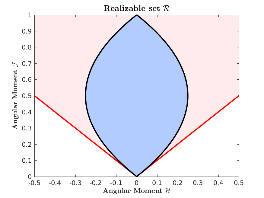
Here we consider a two-moment model for particles governed by Fermi-Dirac statistics. It is well known from the two-moment model for particles governed by Maxwell-Boltzmann statistics (“classical” particles with ), that the particle density is nonnegative and the magnitude of the flux vector is bounded by the particle density. (There are further constraints on the components of the Eddington tensor [22].) Furthermore, the set of realizable moments generated by the particle density and flux vector constitutes a convex cone [26]. In the fermionic case, there is also an upper bound on the distribution function (e.g., ) because Pauli’s exclusion principle prevents particles from occupying the same microscopic state. The fermionic two-moment model has recently been studied theoretically in the context of maximum entropy closures [27, 28, 29] and Kershaw-type closures [4]. Because of the upper bound on the distribution function, the algebraic constraints on realizable moments differ from the classical case with no upper bound, and can lead to significantly different dynamics when the occupancy is high (i.e., when is close to its upper bound). In the fermionic case, the set of realizable moments generated by the particle density and flux vector is also convex. It is “eye-shaped” (as will be shown later; cf. Figure 1 in Section 3) and tangent to the classical realizability cone on the end representing low occupancy, but is much more restricted for high occupancy.
In this paper, the two-moment model is discretized in space using high-order Discontinuous Galerkin (DG) methods (e.g., [30, 31]). DG methods combine elements from both spectral and finite volume methods and are an attractive option for solving hyperbolic partial differential equations (PDEs). They achieve high-order accuracy on a compact stencil; i.e., data is only communicated with nearest neighbors, regardless of the formal order of accuracy, which can lead to a high computation to communication ratio, and favorable parallel scalability on heterogeneous architectures has been demonstrated [32]. Furthermore, they can easily be applied to problems involving curvilinear coordinates (e.g., beneficial in numerical relativity [33]). Importantly, DG methods exhibit favorable properties when collisions with a background are included, as they recover the correct asymptotic behavior in the diffusion limit, characterized by frequent collisions (e.g., [34, 35, 36]). The DG method was introduced in the 1970s by Reed & Hill [37] to solve the neutron transport equation, and has undergone remarkable developments since then (see, e.g., [38] and references therein).
We are concerned with the development and application of DG methods for the fermionic two-moment model that can preserve the aforementioned algebraic constraints and ensure realizable moments, provided the initial condition is realizable. Our approach is based on the constraint-preserving (CP) framework introduced in [1], and later extended to the Euler equations of gas dynamics in [2]. (See, e.g., [39, 40, 26, 41, 42, 43, 44] for extensions and applications to other systems.) The main ingredients include (1) a realizability-preserving update for the cell averaged moments based on forward Euler time stepping, which evaluates the polynomial representation of the DG method in a finite number of quadrature points in the local elements and results in a Courant-Friedrichs-Lewy (CFL) condition on the time step; (2) a limiter to modify the polynomial representation to ensure that the algebraic constraints are satisfied point-wise without changing the cell average of the moments; and (3) a time stepping method that can be expressed as a convex combination of Euler steps and therefore preserves the algebraic constraints (possibly with a modified CFL condition). As such, our method is an extension of the realizability-preserving scheme developed by Olbrant el al. [26] for the classical two-moment model.
The DG discretization leaves the temporal dimension continuous. This semi-discretization leads to a system of ordinary differential equations (ODEs), which can be integrated with standard ODE solvers (i.e., the method of lines approach to solving PDEs). We use implicit-explicit (IMEX) Runge-Kutta (RK) methods [45, 46] to integrate the two-moment model forward in time. This approach is motivated by the fact that we can resolve time scales associated with particle streaming terms in the moment equations, which will be integrated with explicit methods, while terms associated with collisional interactions with the background induce fast time scales that we do not wish to resolve, and will be integrated with implicit methods. This splitting has some advantages when solving kinetic equations since the collisional interactions may couple across momentum space, but are local in position space, and are easier to parallelize than a fully implicit approach.
The CP framework of [1] achieves high-order (i.e., greater than first-order) accuracy in time by employing strong stability-preserving explicit Runge-Kutta (SSP-RK) methods [5, 47], which can be written as a convex combination of forward Euler steps. Unfortunately, this strategy to achieve high-order temporal accuracy does not work as straightforwardly for standard IMEX Runge-Kutta (IMEX-RK) methods because implicit SSP Runge-Kutta methods with greater than first-order accuracy have time step restrictions similar to explicit methods [47]. To break this “barrier,” recently proposed IMEX-RK schemes [48, 49] have resorted to first-order accuracy in favor of the SSP property in the standard IMEX-RK scheme, and recover second-order accuracy with a correction step.
We consider the application of the correction approach to the two-moment model. However, with the correction step from [48] we are unable to prove the realizability-preserving property without invoking an overly restrictive time step. With the correction step from [49] the realizability-preserving property is guaranteed with a time step comparable to that of the forward Euler method applied to the explicit part of the scheme, but the resulting scheme performs poorly in the asymptotic diffusion limit. Because of these challenges, we resort to first-order temporal accuracy, and propose IMEX-RK schemes that are convex-invariant with a time step equal to that of forward Euler on the explicit part, perform well in the diffusion limit, and reduce to a second-order SSP-RK scheme in the streaming limit (no collisions with the background material).
The realizability-preserving property of the DG-IMEX scheme depends sensitively on the adopted closure procedure. The explicit update of the cell average can, after employing the simple Lax-Friedrichs flux and imposing a suitable CFL condition on the time step, be written as a convex combination. Realizability of the updated cell average is then guaranteed from convexity arguments [1], provided all the elements in the convex combination are realizable. Realizability of individual elements in the convex combination is conditional on the closure procedure (components of the Eddington tensor must be computed to evaluate numerical fluxes). We prove that each element in the convex combination is realizable provided the moments involved in expressing the elements are moments of a distribution function satisfying the bounds implied by Fermi-Dirac statistics (i.e., ). For algebraic two-moment closures, which we consider, the so-called Eddington factor is given by an algebraic expression depending on the evolved moments and completely determines the components of the Eddington tensor. Realizable components of the Eddington tensor demand that the Eddington factor satisfies strict lower and upper bounds (e.g., [22, 27]). We discuss algebraic closures derived from Fermi-Dirac statistics that satisfy these bounds, and demonstrate with numerical experiments that the DG-IMEX scheme preserves realizability of the moments when these closures are used. We also demonstrate that further approximations to algebraic two-moment closures for modeling particle systems governed by Fermi-Dirac statistics may give results that are incompatible with a bounded distribution and, therefore, unphysical. The example we consider is the Minerbo closure [19], which can be obtained as the low occupancy limit of the maximum entropy closure of Cernohorsky & Bludman [3].
The paper is organized as follows. In Section 2 we present the two-moment model. In Section 3 we discuss moment realizability for the fermionic two-moment model, while algebraic moment closures are discussed in Section 4. In Section 5 we briefly introduce the DG method for the two-moment model, while the (convex-invariant) IMEX time stepping methods we use are discussed in Section 6. The main results on the realizability-preserving DG-IMEX method for the fermionic two-moment model are worked out in Sections 7 and 8. In Section 8 we also discuss the realizability-enforcing limiter. Numerical results are presented in Section 9, and summary and conclusions are given in Section 10. Additional details on the IMEX schemes are provided in Appendices.
2 Mathematical Model
In this section we give a summary of the mathematical model.
2.1 Boltzmann Equation
We consider approximate solutions to the Boltzmann equation for the transport of massless particles through a static material in Cartesian geometry, which, after scaling to dimensionless units, can be written as
| (2) |
where the distribution function gives the number of particles propagating in the direction , with energy , at position and time . Here we use spherical momentum space coordinates , and the unit vector (independent of and ) is parallel to the particle three-momentum . We also define the energy-position coordinates . On the right-hand side of Eq. (2), is the ratio of the particle mean-free path (due to interactions with a background) to some characteristic length scale of the problem. In opaque regions, , while for free streaming particles, . The collision operator, which models emission, absorption, and isotropic and elastic scattering, is given by
| (3) |
where is the ratio of the absorption opacity to the total opacity , and is the scattering opacity. In particular, models pure emission and absorption, while models pure scattering. In general, and (and and ) depend on . The equilibrium distribution function is denoted by . Here, we consider transport of Fermions (e.g., neutrinos), so the equilibrium distribution function takes the form
| (4) |
where the temperature and the chemical potential depend on properties of the background.
2.2 Angular Moment Equations: Two-Moment Model
The Boltzmann equation is often too expensive to solve directly. Instead, approximate equations for angular moments of the distribution function are solved. To this end, we define the angular moments of the distribution function
| (5) |
We refer to (zeroth moment) as the particle density, (first moment) as the particle flux, and (second moment) as the stress tensor. Note that the moments defined in Eq. (5) are spectral moments (depending on energy as well as position and time). The grey moments (depending only on position and time) are obtained by integration over energy:
| (6) |
Taking the zeroth and first moments of Eq. (2) gives the two-moment model, comprising a system of conservation laws with sources
| (7) |
where and . Components of the fluxes in each coordinate direction are , where is the unit vector parallel to the th coordinate direction. On the right-hand side of Eq. (7), the source term is
| (8) |
where and , with the identity matrix.
In order to close the system given by Eq. (7), the components of the stress tensor must be related to the lower moments through a closure procedure. To this end, Levermore [22] defined the Eddington tensor and assumed that the radiation field is symmetric about a preferred direction so that
| (9) |
where is the Eddington factor. The two-moment model is then closed once the Eddington factor is determined from and . We will return to the issue of determining the Eddington factor in Section 4.
3 Moment Realizability for the Fermionic Two-Moment Model
Our goal is to simulate massless fermions (e.g., neutrinos) and study their interactions with matter. The principal objective is to obtain the fermionic distribution function (or moments of as in the two-moment model employed here). The Pauli exclusion principle requires the distribution function to satisfy the condition , which puts restrictions on the admissible values for the moments of . In this paper, we seek to design a numerical method for solving the system of moment equations given by Eq. (7) that preserves realizability of the moments; i.e., the moments evolve within the set of admissible values as dictated by Pauli’s exclusion principle. (Since we are only concerned with the angular dependence of in this section, we simplify the notation by suppressing the and dependence and write .)
We begin with the following definition of moment realizability.
Definition 1.
The moments are realizable if they can be obtained from a distribution function satisfying . The set of all realizable moments is
| (10) |
where we have defined the concave function .
Remark 1.
Lemma 1.
The realizable set is convex.
Proof.
Let and be two arbitrary elements in , and let , with . The first component of is
Since , it follows that . Concavity of implies that
Hence, . ∎
Figure 1 illustrates the geometry of the convex set in the -plane (light blue region). The boundary (black curves) is given by . The realizable domain of positive distribution functions, (no upper bound on ), which is a convex cone defined by
| (11) |
is partially shown as the light red region above the red lines, which mark the boundary of (denoted ). The realizable set is a bounded subset of .
For the realizability-preserving scheme developed in Section 7, we state some additional results. Lemma 2 is used to help prove the realizability-preserving property of explicit steps in the IMEX scheme, while Lemmas 3 and 4 are used to prove realizability-preserving properties of implicit steps.
Lemma 2.
Let and be moments defined as in Eq. (5) with distribution functions and , respectively, such that . Let , where is an arbitrary unit vector, and . Then
Proof.
The components of are
where and . Then, since , it follows that . ∎
Lemma 3.
Proof.
Lemma 4.
4 Algebraic Moment Closures
The two-moment model given by Eq. (5) is not closed because of the appearance of the second moments (the normalized pressure tensor). Algebraic moment closures for the two-moment model are computationally efficient as they provide the Eddington factor in Eq. (9) in closed form as a function of the density and the flux factor . For this reason they are used in applications where transport plays an important role, but where limited computational resources preclude the use of higher fidelity models. Examples include simulation of neutrino transport in core-collapse supernovae [50] and compact binary mergers [51]. Algebraic moment closures in the context of these aforementioned applications have also been discussed elsewhere (e.g., [52, 53, 54, 55, 56]). Here we focus on properties of the algebraic closures that are critical to the development of numerical methods for the two-moment model of fermion transport. For the algebraic closures we consider, the Eddington factor in Eq. (9) can be written in the following form [3]
| (13) |
where the closure function depends on the specifics of the closure procedure. We will consider two basic closure procedures in more detail below: the maximum entropy (ME) closure and the Kershaw (K) closure.
In the low occupancy limit (), the Eddington factor in Eq. (13) depends solely on ; i.e.,
| (14) |
This for of yields a moment closure that is suitable for particle systems obeying Maxwell-Boltzmann statistics.
4.1 Maximum Entropy (ME) Closure
The ME closure constructs an approximation of the angular distribution as a function of and [3, 27]. The ME distribution is found by maximizing the entropy functional, which for particles obeying Fermi-Dirac statistics is given by
| (15) |
subject to the constraints
| (16) |
The solution that maximizes Eq. (15) takes the general form [3]
| (17) |
where the Lagrange multipliers and are implicit functions of and . The ME distribution function satisfies , but and are unconstrained. Specification of and from gives , and any number of moments can in principle be computed. Importantly, for the maximum entropy problem to be solvable, we must have [27].
To arrive at an algebraic form of the ME closure, Cernohorsky & Bludman [3] postulate (but see [27]) that, as a function of the flux saturation
| (18) |
the closure function is independent of and can be written explicitly in terms of the inverse Langevin function. To avoid inverting the Langevin function for , they provide a polynomial fit (accurate to ) given by
| (19) |
More recently, Larecki & Banach [27] have shown that the explicit expression given in [3] is not exact and provide another approximate expression
| (20) |
which is accurate to within . On the interval , the curves given by Eqs. (19) and (20) lie practically on top of each other. The closure functions given by Eqs. (19) and (20), together with the Eddington factor in Eq. (13) and the pressure tensor in Eq (9), constitute the algebraic maximum entropy closures for fermionic particle systems considered in this paper. We will refer to the ME closures with and as the CB (Cernohorsky & Bludman) and BL (Banach & Larecki) closures, respectively.
We also note that using the closure function given by Eq. (19) with the low occupancy Eddington factor in Eq (14) results in the algebraic maximum entropy closure attributed to Minerbo [19], which is currently in use in simulation of neutrino (fermion) transport in the aforementioned nuclear astrophysics applications. In a recent comparison of algebraic (or analytic) closures for the two-moment model applied to neutrino transport around proto-neutron stars, Murchikova et al. [56] obtained nearly identical results when using the closures of CB and Minerbo. For these reasons, we include the Minerbo closure in the subsequent discussion and in the numerical tests in Section 9.
4.2 Kershaw (K) Closure
Another algebraic closure we consider is a Kershaw-type closure [18], developed for fermion particle systems in [4]. The basic principle of the Kershaw closure for the two-moment model is derived from the fact that the realizable set generated by the triplet of scalar moments
| (21) |
is convex. For the moments in Eq. (21), the realizable set is the set of moments obtained from distribution functions satisfying . (The moments in Eq. (21) are the unique moments obtained from the moments in Eq. (5) under the assumption that the distribution function is isotropic about a preferred direction, and is the cosine of the angle between this preferred direction and the particle propagation direction given by .)
For a bounded distribution , it is possible to show (e.g., [28]) that the second moment satisfies
| (22) |
where , , and is the flux saturation defined in Eq. (18). By convexity of the realizable set generated by the moments in Eq. (21), the convex combination
| (23) |
with , is realizable whenever . The Kershaw closure for the two-moment model is then obtained from Eq. (23) with the additional requirement that it be correct in the limit of isotropic distribution functions; i.e., . One choice for , which leads to a strictly hyperbolic and causal two-moment model (and a particularly simple closure function) [4], is , so that , where
| (24) |
and the Kershaw closure function is given by
| (25) |
For multidimensional problems, the Kershaw closure is obtained by using the Eddington factor in Eq. (24) in Eq. (9). Finally, we point out that for the two-moment Kershaw closure (see [4] for details), a distribution function , satisfying , and reproducing the moments , , and , can be written explicitly in terms of Heaviside functions.
4.3 Realizability of Algebraic Moment Closures
It is not immediately obvious that all the algebraic moment closures discussed above are suitable for designing realizability-preserving methods for the two-moment model of fermion transport. In particular, the realizability-preserving scheme developed in this paper is based on the result in Lemma 2, which must hold for the adapted closure. The Kershaw closure is consistent with a bounded distribution, , and should be well suited, but the algebraic ME closures are based on approximations to the closure function, and we need to consider if these approximate closures remain consistent with the assumed bounds on the underlying distribution function. To this end, we rely on results in [22, 27] (see also [18, 57]), which state that realizability of the moment triplet (with given by Eq. (9)), is equivalent to the following requirement for the Eddington factor
| (26) |
Fortunately, these bounds are satisfied by the algebraic closures based on Fermi-Dirac statistics. (Note that for the bounds in Eq. (26) limit to the bounds for positive distributions given by Levermore [22]; i.e., .)
In Figure 2, we plot the Eddington factor versus the flux factor for the various algebraic closures discussed above and for different values of : (upper left panel), (upper right panel), (lower left panel), and (lower right panel). The lower and upper bounds on the Eddington factor for realizable closures ( and , respectively) are also plotted. We note that for all the closures, the Eddington factor as .
When , the maximum entropy closures (CB, BL, and Minerbo) are practically indistinguishable, while the Eddington factor of the Kershaw closure is larger than that of the other closures over most of the domain. When , the Eddington factor for the closures based on Fermi-Dirac statistics (CB, BL, and Kershaw) remain close together, while the Eddington factor for the Minerbo closure is larger than the other closures for . The Eddington factor for all closures remain between and when and .
When , the Eddington factor for the closures based on Fermi-Dirac statistics remain close together and within the bounds in Eq. (26). The dependence of the Eddington factor on for the Minerbo closure differs from the other closures (i.e., increases vs decreases with increasing ), and exceeds for . When , the Eddington factor of the CB and BL closures (indistinguishable) and the Kershaw closure remain within the bounds given in Eq. (26). The Eddington factor of the Minerbo closure is nearly flat, and exceeds for .

 |

 |
We have also checked numerically that for all the algebraic closures based on Fermi-Dirac statistics (CB, BL, and Kershaw), the bounds on the Eddington factor in Eq. (26) holds for all . Thus, we conclude that these closures are suited for development of realizability-preserving numerical methods for the two-moment model of fermion transport.
In Figure 3, we further illustrate properties of the algebraic closures by plotting as defined in Lemma 2 for the maximum entropy closures of CB and Minerbo. In both panels, we plot constructed from randomly selected pairs (each blue dot represents one realization of ). Results for the maximum entropy closure of CB are plotted in the left panel, while results for the Minerbo closure are plotted in the right panel. As expected for the closure consistent with moments of Fermi-Dirac distributions (CB), we find . For the Minerbo closure, which is consistent with positive distributions, is not confined to .

 |
5 Discontinuous Galerkin Method
Here we briefly outline the DG method for the moment equations. (See, e.g., [30], for a comprehensive review on the application of DG methods to solve hyperbolic conservation laws.) Since we do not include any physics that couples the energy dimension, the particle energy is simply treated as a parameter. For notational convenience, we will suppress explicit energy dependence of the moments. Employing Cartesian coordinates, we write the moment equations in spatial dimensions as
| (27) |
where is the coordinate along the th coordinate dimension. We divide the spatial domain into a disjoint union of open elements , so that . We require that each element is a -dimensional box in the logical coordinates; i.e.,
| (28) |
with surface elements denoted . We let denote the volume of an element
| (29) |
We also define as the coordinates orthogonal to the th dimension, so that as a set . The width of an element in the th dimension is .
We let the approximation space for the DG method, , be constructed from the tensor product of one-dimensional polynomials of maximal degree . Note that functions in can be discontinuous across element interfaces. The semi-discrete DG problem is to find (which approximates in Eq. (27)) such that
| (30) |
for all and all .
In Eq. (30), is a numerical flux, approximating the flux on the surface of with unit normal along the th coordinate direction. It is evaluated with a flux function using the DG approximation from both sides of the element interface; i.e.,
| (31) |
where superscripts in the arguments of indicate that the function is evaluated to the immediate left/right of . In this paper we use the simple Lax-Friedrichs (LF) flux given by
| (32) |
where is the largest eigenvalue (in absolute value) of the flux Jacobian . For particles propagating at the speed of light, we can simply take (i.e., the global LF flux).
6 Convex-Invariant IMEX Schemes
In this section we discuss the class of IMEX schemes that are used for the realizability-preserving DG-IMEX method developed in Section 7 (see also A for additional details). The semi-discretization of the moment equations with the DG method given by Eq. (30) results in a system of ordinary differential equations (ODEs) of the form
| (33) |
where are the degrees of freedom evolved with the DG method; i.e., for a test space spanned by , we let
| (34) |
Thus, for , the first components of are the cell averaged moments. In Eq. (33), the transport operator corresponds to the second and third term on the left-hand side of Eq. (30), while the collision operator corresponds to the right-hand side of Eq. (30).
Eq. (33) is to be integrated forward in time with an ODE integrator. Since the realizable set is convex, convex-invariant schemes can be used to design realizability-preserving schemes for the two-moment model.
Definition 2.
Given sufficient conditions, a convex-invariant time integration scheme preserves the constraints of a model if the set of admissible states satisfying the constraints forms a convex set.
As an example, high-order explicit strong stability-preserving Runge-Kutta (SSP-RK) methods form a class of convex-invariant schemes.
6.1 Second-Order Accurate, Convex-Invariant IMEX Schemes
In many applications, collisions with a background induce stiffness () in regions of the computational domain that must be treated with implicit methods. Meanwhile, the time scales induced by the transport term can be treated with explicit methods. This motivates the use of IMEX methods [45, 46]. Our goal is to employ IMEX schemes that preserve realizability of the moments, subject only to a time step governed by the explicit transport operator and comparable to the time step required for numerical stability of the explicit scheme. We seek to achieve this goal with convex-invariant IMEX schemes.
Unfortunately, high-order (second or higher order temporal accuracy) convex-invariant IMEX methods with time step restrictions solely due to the transport operator do not exist (see for example Proposition 6.2 in [47], which rules out the existence of implicit SSP-RK methods of order higher than one). To overcome this barrier, Chertock et al. [48] presented IMEX schemes with a correction step. These schemes are SSP but only first-order accurate within the standard IMEX framework. The correction step is introduced to recover second-order accuracy. However, the correction step in [48] involves both the transport and collision operators, and we have found that, when applied to the fermionic two-moment model, realizability is subject to a time step restriction that depends on in a way that becomes too restrictive for stiff problems. More recently, Hu et al. [49], presented similar IMEX schemes for problems involving BGK-type collision operators, but with a correction step that does not include the transport operator. In this case, the scheme is convex-invariant, subject only to time step restrictions stemming from the transport operator, which is more attractive for our target application. These second-order accurate, -stage IMEX schemes take the following form [49]
| (35) | ||||
| (36) | ||||
| (37) |
where, as in standard IMEX schemes, and , components of matrices and , respectively, and the vectors and must satisfy certain order conditions [46]. The coefficient in the correction step is positive, and is the Fréchet derivative of the collision term evaluated at . For second-order accuracy, can be evaluated using any of the stage values (, , or ). For second-order temporal accuracy, the order conditions for the IMEX scheme in Eqs. (35)-(37) are [49]
| (38) |
and
| (39) |
where and are given in A. For globally stiffly accurate (GSA) IMEX schemes, and for , so that [45]. This property is beneficial for very stiff problems and also simplifies the proof of the realizability-preserving property of the DG-IMEX scheme given in Section 7, since it eliminates the assembly step in Eq. (36).
Hu et al. [49] rewrite the stage values in Eq. (35) in the following form
| (40) |
where , and are computed from and (see A). In Eq. (40), . Two types of IMEX schemes are considered: type A [46, 58] and type ARS [45]. For IMEX schemes of type A, the matrix is invertible. For IMEX schemes of type ARS, the matrix can be written as
where is invertible. In writing the stages in the IMEX scheme in the general form given by Eq. (40), it should be noted that for IMEX schemes of Type A, and for IMEX schemes of Type ARS [49]. Type A schemes can be made convex-invariant by requiring
| (41) |
Similarly, type ARS schemes can be made convex-invariant by requiring
| (42) |
Coefficients were given in [49] for GSA schemes of type A with and type ARS with . (It was also proven that and are the necessary number of stages needed for GSA second-order convex-invariant IMEX schemes of type A and type ARS, respectively.)
In Eq. (40), the explicit part of the IMEX scheme has been written in the so-called Shu-Osher form [5]. For the scheme to be convex-invariant, the coefficients must also satisfy . Then, if the expression inside the square brackets in Eq. (40) — which is in the form of a forward Euler update with time step — is in the (convex) set of admissible states for all , and , it follows from convexity arguments that the entire sum on the right-hand side of Eq. (40) is also admissible. Thus, if the explicit update with the transport operator is admissible for a time step , the IMEX scheme is convex-invariant for a time step , where
| (43) |
Here, is the CFL condition, relative to , for the IMEX scheme to be convex-invariant. It is desirable to make as large (close to ) as possible. Note that for to be admissible also requires the implicit solve (equivalent to implicit Euler) to be convex-invariant. In [49], Hu et al. provide examples of GSA, convex-invariant IMEX schemes of type A (see scheme PA2 in A) and type ARS. In A, we provide another example of a GSA, convex-invariant IMEX scheme of type A (scheme PA2+), with a larger (a factor of about larger).
6.2 Convex-Invariant, Diffusion Accurate IMEX Schemes
Unfortunately, the correction step in Eq. (37) deteriorates the accuracy of the IMEX scheme when applied to the moment equations in the diffusion limit. The diffusion limit is characterized by frequent collisions () in a purely scattering medium (), and exhibits long-time behavior governed by (e.g., [59])
| (44) |
Here the time derivative term in the equation for the particle flux has been dropped (formally ) so that, to leading order in , the second equation in Eq. (44) states a balance between the transport term and the collision term. Furthermore, in the diffusion limit, the distribution function is nearly isotropic so that and . The absence of the transport operator in the correction step in Eq. (37), destroys the balance between the transport term and the collision term. We demonstrate the inferior performance of IMEX schemes with this correction step in the diffusion limit in Section 9.1. We have also implemented and tested one of the IMEX schemes in Chertock et al. [48] (not included in Section 9.1), where the transport operator is part of the correction step, and found it to perform very well in the diffusion limit. However, we have not been able to prove the realizability-preserving property with this approach without invoking a too severe time step restriction. We therefore proceed to design convex-invariant IMEX schemes without the correction step that perform well in the diffusion limit. We limit the scope to IMEX schemes of type ARS. (It can be shown that IMEX schemes of type A conforming to Definition 3 below do not exist; cf. C.)
We take a heuristic approach to determine conditions on the coefficients of the IMEX scheme to ensure it performs well in the diffusion limit. We leave the spatial discretization unspecified. Define the vectors
| (45) |
(The components of and can, e.g., be the cell averages evolved with the DG method.) We can then write the stages of the IMEX scheme in Eq. (35) applied to the particle density equation as
| (46) |
where is a vector of length containing all ones, and the divergence operator acts individually on the components of . Similarly, for the particle flux equation we have
| (47) |
In the context of IMEX schemes, the diffusion limit (cf. the second equation in (44)) implies that the relation should hold. Define the pseudoinverse of the implicit coefficient matrix for IMEX schemes of type ARS as
Then, for the stages ,
| (48) |
where is the th column of the identity matrix and we have introduced the expansion . For to be accurate in the diffusion limit, we require that
| (49) |
(The case is trivial and does not place any constraints on the components of and .) If Eq. (49) holds, then
| (50) |
which approximates a diffusion equation for with the correct diffusion coefficient . (For a GSA IMEX scheme without the correction step, .)
Unfortunately, the “diffusion limit requirement" in Eq. (49), together with the order conditions given by Eqs. (38) and (39) (with ), and the positivity conditions on and , result in too many constraints to obtain a second-order accurate convex-invariant IMEX scheme.11 1 It was shown in [49] — without the diffusion limit requirement — that the minimum number of stages for convex-invariant IMEX schemes of type ARS is four.) We are also concerned about increasing the number of stages, and thereby the number of implicit solves, since the implicit solve will dominate the computational cost of the IMEX scheme with more realistic collision operators (e.g., inelastic scattering). To reduce the number of constraints and accommodate accuracy in the diffusion limit, we relax the requirement of overall second-order accuracy of the IMEX scheme. Instead, we only require the scheme to be second-order accurate in the streaming limit (). This gives the order conditions
| (51) |
where the first condition (consistency condition) is required for first-order accuracy. We then seek to design IMEX schemes of Type ARS conforming to the following working definition
Definition 3.
Let PD-IMEX be an IMEX scheme satisfying the following properties:
- 1.
Consistency of the implicit coefficients
(52) - 2.
Second-order accuracy in the streaming limit; i.e., satisfies Eq. (51).
- 3.
Convex-invariant; i.e. satisfies Eq. (42), with , for , and .
- 4.
Well-behaved in the diffusion limit; i.e., satisfies Eq. (49).
- 5.
Less than four stages ().
- 6.
Globally stiffly accurate (GSA): and .
Fortunately, IMEX schemes of type ARS satisfying these properties are easy to find, and we provide an example with (two implicit solves) in A (scheme PD-ARS; see B for further details). In the streaming limit, this scheme is identical to the optimal second-order accurate SSP-RK method [47]. It is also very similar to the scheme given in [60] (see scheme PC2 in A), which is also a GSA IMEX scheme of type ARS with . Scheme PC2 is second-order in the streaming limit, has been demonstrated to work well in the diffusion limit [60, 61], and satisfies the positivity conditions in Eq. (42). However, (our primary motivation for finding an alternative). In Section 9, we show numerically that the accuracy of scheme PD-ARS is comparable to the accuracy of scheme PC2.
6.3 Absolute Stability
Here we analyze the absolute stability of the proposed IMEX schemes, PA2+ and PD-ARS (given in A), following [49]. As is commonly done, we do this in the context of the linear scalar equation
| (53) |
where and . On the right-hand side of Eq. (53), the first (oscillatory) term is treated explicitly, while the second (damping) term is treated implicitly. The IMEX schemes can then be written as , where is the amplification factor of the scheme, , and . Stability of the IMEX scheme requires . The stability regions of PA2+ and PD-ARS are plotted in Figure 4. As can be seen from the figures, the absolute stability region of both schemes increases with increasing (increased damping). For a given , the stability region of PD-ARS is larger than that of PA2+. In the linear model in Eq. (53), a time step that satisfies the absolute stability for the explicit part of the IMEX scheme () fulfills the stability requirement for the IMEX scheme as whole (). This holds for all PD-ARS schemes with .

 |
7 Realizability-Preserving DG-IMEX Scheme
We proceed to develop realizability-preserving DG schemes for the two-moment model based on the IMEX schemes discussed in the previous section (cf. Eqs. (35)-(37)). Following the framework in [2] for high-order DG schemes, the realizability-preserving DG-IMEX scheme is designed to preserve realizability of cell averages over a time step in each element . Realizability of the cell average is leveraged to limit the polynomial approximation in the stages of the IMEX scheme. If the polynomial approximation is not realizable in a finite number of points in , the high-order components are damped (see Section 8). The main result of this section is stated in Theorem 1. The realizability-preserving property of the DG-IMEX scheme is stated in Theorem 2 in Section 8, after the discussion of the limiter.
The cell average of the moments is defined as
| (54) |
With in Eq. (30), the stage values for the cell average in the IMEX scheme (cf. Eq. (40)) can be written as
| (55) |
where , , ,
| (56) |
and . The cell average of the divergence operator is
| (57) |
We first establish conditions for realizability of the stage values in Eq. (55).
Lemma 5.
Let satisfy Eq. (55). Assume that . Then, , for .
Proof.
We next establish conditions under which .
Lemma 6.
Let be a set of strictly positive constants satisfying . If for each ,
| (58) | ||||
is realizable, then .
Proof.
It is easy to show that can be expressed as the convex combination
| (59) |
The result follows immediately. ∎
Remark 3.
Next, we establish conditions for which Eq. (58) holds. To this end, let denote the -point Gauss-Lobatto (GL) quadrature rule on the interval , with points
| (60) |
and weights , normalized so that . (The hat is used to denote the GL rule, which includes the endpoints of the interval .) This quadrature integrates polynomials in with degree exactly. If is represented by such polynomials, then
| (61) |
where for simplicity of notation, we have suppressed the explicit dependence on to denote . In each element, we also denote and . Similarly, the solution on to the immediate left of is denoted , and the solution on to the immediate right of is denoted .
Using Eq. (61), can be expressed as the convex combination
| (62) |
where . (With the GL quadrature rule in Eq. (61), ). The following Lemma establishes sufficient conditions for realizability of , and hence .
Lemma 7.
Assume that for all and all . Let the time step be chosen so that . Let the numerical flux be given by the Lax-Friedrichs flux in Eq. (32) with . Then .
Proof.
In Eq. (62), is expressed as a convex combination. By assumption, (). Thus it remains to show that
is realizable. Using the Lax-Friedrichs flux in Eq. (32), with (), it is straightforward to show that
| (63) |
where
and ; cf. Lemma 2. Since , is expressed as a convex combination of , , and . By assumption, , , , , which immediately implies realizability of . Realizability of and follows by invoking Lemma 2. This completes the proof. ∎
Remark 4.
For the IMEX scheme to be realizability-preserving it is sufficient to set the time step such that
| (64) |
where is defined in (43).
Remark 5.
Lemma (7) is proven without specification of . In the numerical scheme, we need to be realizable in the quadrature set used to approximate the integral over in Eq. (58). (Typically, is a tensor product of Gauss-Legendre quadrature points.) We thus require to be realizable in the quadrature set , where , and are the GL quadrature points.
Remark 6.
For GSA IMEX schemes, . For IMEX schemes incorporating the correction step in Eq. (37), the cell average at is obtained by solving
| (65) |
where and are defined in Eq. (8). For these IMEX schemes, realizability of is established by the following lemma.
Lemma 8.
Suppose that and is obtained by solving Eq. (65). Then .
Proof.
The result follows immediately from Lemma 4. ∎
Remark 7.
For IMEX scheme PD-ARS (B), which does not invoke the correction step (i.e., ), .
We are now ready to state the main result of this section.
Theorem 1.
8 Realizability-Enforcing Limiter
Condition 2 of Theorem 1 requires that the polynomial approximation () is realizable in every point in the quadrature set . Following Zhang & Shu [1] we use the limiter in [62] to enforce the bounds on the zeroth moment . We replace the polynomial with the limited polynomial
| (66) |
where the limiter parameter is given by
| (67) |
with and , and
| (68) |
In the next step, we ensure realizability of the moments by following the framework of [2], developed to ensure positivity of the pressure when solving the Euler equations of gas dynamics. We let . Then, if lies outside for any quadrature point , i.e., , there exists an intersection point of the straight line, , connecting and evaluated in the troubled quadrature point , denoted , and the boundary of . This line is given by the convex combination
| (69) |
where , and the intersection point is obtained by solving for , using the bisection algorithm22 2 In practice, needs not be accurate to many significant digits, and the bisection algorithm can be terminated after a few iterations.. We then replace the polynomial representation , where
| (70) |
and is the smallest obtained in the element by considering all the troubled quadrature points. This limiter is conservative in the sense that it preserves the cell-average .
The realizability-preserving property of the DG-IMEX scheme results from the following theorem.
Theorem 2.
9 Numerical Tests
In this section we present numerical results obtained with the DG-IMEX scheme developed in this paper. The first set of tests (Section 9.1) are included to compare the time integration schemes in various regimes. We are not concerned with moment realizability in Section 9.1, and we do not apply the realizability-enforcing limiter in these tests. The tests in Sections 9.2 and 9.3 are designed specifically to demonstrate the robustness of the scheme to dynamics near the boundary of the realizable set . The test in Section 9.4 (Homogeneous Sphere) is of astrophysical interest. Here we consider moment realizability and compare results obtained with various moment closures.
9.1 Problems with Known Smooth Solutions
To compare the accuracy of the IMEX schemes, we present results from smooth problems in streaming, absorption, and scattering dominated regimes in one spatial dimension. For all tests in this subsection, we use third order accurate spatial discretization (polynomials of degree ) and we employ the maximum entropy closure in the low occupancy limit (i.e., the Minerbo closure). We compare results obtained using IMEX schemes proposed here (PA2+ and PD-ARS) with IMEX schemes from Hu et al. [49] (PA2), McClarren et al. [60] (PC2), Pareschi & Russo [46] (SSP2332), and Cavaglieri & Bewley [63] (RKCB2). In the streaming test, we also include results obtained with second-order and third-order accurate explicit strong stability-preserving Runge-Kutta methods [47] (SSPRK2 and SSPRK3, respectively). See A for further details. The time step is set to .
When comparing the numerical results to analytic solutions, errors are computed in the -error norm. We compare results either in the absolute error () or the relative error (), defined for a scalar quantity (approximating ) as
| (71) |
and
| (72) |
respectively. The integrals in Eqs. (71) and (72) are computed with a simple -point equal weight quadrature.
9.1.1 Sine Wave: Streaming
The first test involves the streaming part only, and does not include any collisions (). We consider a periodic domain , and let the initial condition be given by
| (73) |
We evolve until , when the sine wave has completed 10 crossings of the computational domain. We vary the number of elements () from to and compute errors for various time stepping schemes.
In Figure 5, the absolute error for the number density is plotted versus (see figure caption for details). Errors obtained with SSPRK3 are smallest and decrease as (cf. bottom black dash-dot reference line), as expected for a scheme combining third-order accurate time stepping with third-order accurate spatial discretization. For all the other schemes, using second-order accurate explicit time stepping, the error decreases as . Among the second-order accurate methods, SSP2332 has the smallest error, followed by RKCB2. Errors for the remaining schemes (including SSPRK2) are indistinguishable on the plot.

9.1.2 Sine Wave: Damping
The next test we consider, adapted from [64], consists of a sine wave propagating with unit speed in a purely absorbing medium (, ), which results in exponential damping of the wave amplitude. We consider a periodic domain , and let the initial condition () be given as in Eq. (73). For a constant absorption opacity , the analytical solution at is given by
| (74) |
where .
We compute numerical solutions for three values of the absorption opacity (, , and ), and adjust the end time so that , and the initial condition has been damped by factor . Thus, for the sine wave crosses the domain 100 times, while for , it crosses the grid once.
Figure 6 shows convergence results, obtained using different values of , for various IMEX schemes at . Results for , , and are plotted with red, green, and blue lines, respectively (see figure caption for further details). All the second-order accurate schemes (PA2, PA2+, RKCB2, and SSP2332) display second-order convergence rates (cf. bottom, black dash-dot reference line). For , SSP2332 is the most accurate among these schemes, while PA2+ is the most accurate for . On the other hand, PC2 and PD-ARS are indistinguishable and display at most first-order accurate convergence, as expected. (For , PC2 and PD-ARS are the most accurate schemes for and .)

9.1.3 Sine Wave: Diffusion
The final test with known smooth solutions, adopted from [61], is diffusion of a sine wave in a purely scattering medium (, ). The computational domain is periodic, and the initial condition is given by
| (75) |
For a sufficiently high scattering opacity, the moment equations limit to a diffusion equation for the number density (deviations appear at the -level). With the initial conditions in Eq. (75), the analytical solution to the limiting diffusion equation is given by
| (76) |
and . When computing errors for this test, we compare the numerical results obtained with the two-moment model to the analytical solution to the limiting diffusion equation. We compute numerical solutions using three values of the scattering opacity (, , and ), and adjust the end time so that . The initial amplitude of the sine wave has then been reduced by a factor for all values of .


In Figures 7 and 8 we plot the absolute error, obtained using different values of , for various IMEX schemes at . Results for , , and are plotted with red, green, and blue lines, respectively (see figure caption for further details). (Scheme PC2 has been shown to work well for this test [61], but is included here for comparison with the other IMEX schemes.) Schemes PD-ARS, RKCB2, and SSP2332 are accurate for this test, and display third-order accuracy for the number density and second-oder accuracy for . For , the errors do not drop below because of differences between the two-moment model and the diffusion equation used to obtain the analytic solution. For larger values of the scattering opacity, the two-moment model agrees better with the diffusion model, and we observe convergence over the entire range of . Schemes PA2 and PA2+ do not perform well on this test (for reasons discussed in Section 6). For , errors in and decrease with increasing , but for , errors remain constant with increasing over the entire range.
9.2 Packed Beam
Next we consider a one-dimensional test with discontinuous initial conditions. The purpose of this test is to further gauge the accuracy of the two-moment model and demonstrate the robustness of the DG scheme for dynamics close to the boundary of the realizable set . The computational domain is , and the initial condition is obtained from a distribution function given by
| (77) |
so that, with , for , and for , where is a small parameter (). We let , so that the initial conditions are very close to the boundary of the realizable domain (cf. Figure 1). The analytical solution can be easily obtained by solving the transport equation for all angles (independent linear advection equations), and taking the angular moments. The numerical results shown in this section were obtained with the third-order scheme (polynomials of degree and the SSPRK3 time stepper) using elements. The time step is set to
Figure 9 shows results for various times obtained with the two-moment model. In the upper panels we plot the number density, while the number flux density is plotted in the lower panels. Numerical solutions are plotted with solid lines, while the analytical solution is plotted with dashed lines. In the left panels, the algebraic maximum entropy closure of Cernohorsky & Bludman (CB) [3] (cf. Eqs. (13) and (19)) was used, while in the right panels the Minerbo closure (cf. Eqs. (14) and (19)) was used. For this test, the use of the realizability-preserving limiter described in Section 8 was essential in order to avoid numerical problems. For the results obtained with the CB closure, the limiter was enacted whenever moments ventured outside the realizable set given by Eq. (10). For the results obtained with the Minerbo closure, which is not based on Fermi-Dirac statistics, we used a modified limiter, which was enacted when the moments ventured outside the realizable domain of positive distributions; i.e., not bounded by , so that and (e.g., [22]; see red line in Figure 1).
 |
 |
As can be seen in Figure 9, with the CB closure the numerical solution obtained with the two-moment model tracks the analytic solution well, while with the Minerbo closure the numerical solution deviates substantially from the analytic solution. With the Minerbo closure, the solution also evolves outside the realizable domain for Fermi-Dirac statistics.
In the left panel in Figure 10 we plot versus position for various times. With the Minerbo closure, becomes negative in regions of the computational domain (dashed lines), while remains positive for all and the CB closure. In the right panel of Figure 10 we plot the numerical solutions in the -plane. Initially, the moments are located in two points: and , for and , respectively (marked by circles in Figure 10). For , the solutions trace out curves in the -plane, connecting and . With the CB closure, the solution curve (blue points) follows the boundary of the realizable set defined in Eq. (10) (cf. black line in Figure 10). With the Minerbo closure (magenta points), the solution follows a different curve — outside the realizable domain for distribution functions bounded by , but inside the realizable domain of positive distributions (cf. red line in Figure 10). We have also run this test using the algebraic maximum entropy closure of Larecki & Banach [27] and the simpler Kershaw-type closure in [4]. The numerical solutions obtained with both of these closures follow the analytic solution well, and remain within the realizable set . We point out that simply using the realizability-preserving limiter described in Section 8 with the Minerbo closure does not result in a realizability-preserving scheme for Fermi-Dirac statistics because of the properties of this closure discussed in Section 4, and plotted in the right panel of Figure 3.
 |
 |
9.3 Fermion Implosion
The next test is inspired by line source benchmark (cf. [65, 66]), which is a challenging test for approximate transport algorithms. The original line source test consists of an initial delta function particle distribution in radius ; i.e., . For , a radiation front propagates in the radial direction, away from . Apart from capturing details of the exact transport solution, maintaining realizability of the two-moment solution is challenging.
Here, a modified version of the line source — dubbed Fermion Implosion, designed to test the realizability-preserving properties of the two-moment model for fermion transport — is computed on a two-dimensional domain . Instead of initializing with a delta function, we follow the initialization procedure in [66], and approximate the initial condition using an isotropic Gaussian distribution function. However, different from [66], the initial distribution function is bounded , and reaches a minimum in the center of the computational domain (hence implosion)
| (78) |
We set , and evolve to a final time of . We run this test using a grid of elements, polynomials of degree , and the SSPRK2 time stepping scheme with . (There are no collisions included in this test; i.e., .) For comparison, we present results using the algebraic closures of Cernohorsky & Bludman (CB) and Minerbo.
 |
 |
 |
 |
Numerical results for the Fermion Implosion problem are plotted in Figure 11. For , the low-density region in the center of the computational domain is quickly filled in, and a cylindrical perturbation propagates radially away from the center. For the model with the CB closure, this perturbation, seen as a depression in the density relative to the ambient medium, has reached for (upper left panel in Figure 11). The right panel in Figure 11 illustrates the difference in dynamics resulting from the two closures. (We also plot a reference transport solution obtained using the filtered spherical harmonics scheme described in [66]; dashed black lines.33 3 Kindly provided by Dr. Ming Tse Paul Laiu (private communications).) With the CB closure (blue lines), the central density increases towards the maximum value of unity, and an low-density pulse propagates radially. The amplitude of the pulse decreases with time due to the geometry of the problem. For , the peak depression in located around (with ). With the Minerbo closure, the central density continues to increase beyond unity, and reaches a maximum of about at . The central density starts to decrease beyond this point in time, and a steepening pulse propagates radially away from the center. (This pulse is trailing the pulse in the model computed with the CB closure.) At , a discontinuity appears to have formed around , resulting in numerical oscillations. Except for the realizability-enforcing limiter (which is not triggered for this model), no other limiters are used to prevent numerical oscillations. Although the solutions obtained with the two-moment model differ from the reference transport solution, the results obtained with the CB closure are in closer agreement with the transport solution. This is likely because the CB closure is consistent with the bound satisfied by the transport solution in this test. (For tests involving lower occupancies, the CB and Minerbo closures are expected to perform similarly.) In the lower left panel in Figure 11, the moments are plotted in the -plane for the same times as plotted in the upper left panel. (Each dot represents the moments at a specific spatial point and time.) Initially, , and all the moments lie on the line connecting and ; cyan points. With the CB closure (blue points), the moments are confined to evolve inside the realizable domain (black), while with the Minerbo closure, the moments are not confined to , but to the region above the red lines (the realizable domain for moments of positive distribution functions), and this is the reason for the difference in dynamics in the two models. For the model with the CB closure, some moments evolve very close to the boundary of the realizable domain, and the positivity limiter is continuously triggered to damp these moments towards the cell average, which is realizable by the design of the numerical scheme. In the lower right panel in Figure 11 we plot the limiter parameters (solid) and (dashed) (cf. (66) and (70)) versus time for the CB closure model (blue) and the Minerbo closure model (magenta); the minimum over the whole computational domain is plotted. For the CB closure model, the limiter is triggered to prevent both density overshoots and . Late in the simulation (), the minimum value of is around . For the model using the Minerbo closure, the limiter is not triggered ().
9.4 Homogeneous Sphere
The homogeneous sphere test (e.g., [67]) considers a sphere with radius . Inside the sphere (radius ), the absorption opacity and the equilibrium distribution function are set to constant values. The scattering opacity is set to zero in this test (i.e., ). Outside the sphere, the absorption opacity is zero. The steady state solution, obtained by solving the transport equation in spherical symmetry, is given by
| (79) |
where ,
| (80) |
and . Thus, .
Here, this test is computed using a three-dimensional Cartesian domain . Because of the symmetry of the problem, and to save computational resources, we only compute the solution in one octant. On the inner boundaries, we impose reflecting boundary conditions, while we impose ’homogeneous’ boundary conditions on the outer boundary in all three coordinate dimensions; i.e., values for all moments in a boundary element are set equal to the corresponding values in the nearest element just inside . Since this test is computed with Cartesian coordinates using a relatively low spatial resolution (), we have found it necessary to smooth out the opacity over a finite radial extent to avoid numerical artifacts due to a discontinuous absorption opacity. Specifically, we use an absorption opacity of the following form
| (81) |
We set , and compute three versions of this test: one with , , and (Test A), one with , , and (Test B), and one with , , and (Test C). (These values for and result in similar radius for where the optical depth equals in Test B and Test C.) We compute until , when the system has reached an approximate steady state. In all the tests, we use the IMEX scheme PD-ARS with — the least compute-intensive of the convex-invariant IMEX schemes presented here. The main purpose of this test is to compare the results obtained using the different algebraic closures discussed in Section 4.
In Figure 12, we plot results obtained for all tests at : Test A (top panels), Test B (middle panels), and Test C (bottom panels). The particle density and the flux factor (left and right panels, respectively) are plotted versus radius . In each panel, results obtained with the various algebraic closures discussed in Section 4 are plotted: Minerbo (magenta), CB (blue), BL (green), and Kershaw (cyan). The analytical solution is also plotted (dashed black lines).

 |

 |

 |
We find good overall agreement between the results obtained with the two-moment model and the analytical solution. Partly due to the smoothing of the absorption opacity around the surface, the numerical and analytical solutions naturally differ around . Aside from some differences discussed in more detail below, the numerical and analytical solutions — for all values of the absorption opacity and all closures — agree well as tends to zero, as well as when . The results obtained with the maximum entropy closures CB and BL are practically indistinguishable on the plots. This is consistent with the similarity of the Eddington factors for these two closures, as shown in Figure 2. We also find that the results obtained with the fermionic Kershaw closure agree well with the maximum entropy closures based on Fermi-Dirac statistics (CB and BL). From the plots of the particle density (left panels in Figure 12), the results obtained with all the closures, including Minerbo, appear very similar. (For Test A, the particle density obtained with the Minerbo closure deviates the most from the analytic solution inside ; upper left panel). From the plots of the flux factor (right panels in Figure 12), it is evident that the results obtained with the Minerbo closure — the only closure not based on Fermo-Dirac statistics — deviates the most from the analytic solution outside , where the flux factor is consistently higher than the analytical solution for all values of . The fermionic closures (CB, BL, and Kershaw) track the analytic solution better. Similar agreement between the numerical and analytical solutions was reported by Smit et al. [67], when using the CB maximum entropy closure with and an unsmoothed absorption opacity . We also note that our results appear to be somewhat at odds with the results recently reported by Murchikova et al. [56], who compared results obtained with the two-moment model using a large number of algebraic closures for this same problem (albeit using an unsmoothed and slightly different value for the absorption opacity). Murchikova et al. do not plot the particle density, but find essentially no difference in the flux factor and the Eddington factor when comparing results obtained with the maximum entropy closures of Minerbo and Cernohorsky & Bludman (CB).
In Figure 13, we further compare the results obtained when using the Minerbo and CB closures by plotting the solutions to the homogeneous sphere problem for Test C at in the -plane (cf. the realizable domain in Figure 1). The numerical solution at each spatial point is represented by a blue (CB) or magenta (Minerbo) dot in the panels. In the lower two panel we zoom in on the results obtained with the two closures around the top and lower right regions of the realizable domain (lower left and lower right panel, respectively; cf. green boxes in the upper right panel).


 |
As can be seen in the upper panel in Figure 13, the solutions to the homogeneous sphere problem obtained with the two closures trace out distinct curves relative to the realizable domain , whose boundary is indicated by solid black curves in each panel. When using the CB closure, the realizability-preserving DG-IMEX scheme developed here maintains solutions within . When using the Minerbo closure, the appropriate realizable domain is given by (cf. Eq. (11)), whose boundary is indicated by solid red lines in Figure 13, and we find that the numerical solution ventures outside . Near the surface around , the number density slightly exceeds unity (lower left panel), while for larger radii, the computed flux may exceed the value allowed by Fermi-Dirac statistics (lower right panel).
10 Summary and Conclusions
We have developed a realizability-preserving DG-IMEX scheme for a two-moment model of fermion transport. The scheme employs algebraic closures based on Fermi-Dirac statistics and combines a time step restriction (CFL condition), a realizability-enforcing limiter, and a convex-invariant time integrator to maintain point-wise realizability of the moments. Since the realizable domain is a convex set, the realizability-preserving property is obtained from convexity arguments, building on the framework in [1].
In the applications motivating this work, the collision term is stiff in regions of the computational domain, and we have considered IMEX schemes to avoid treating the transport operator implicitly. We have considered two recently proposed second-order accurate, convex-invariant IMEX schemes [48, 49], that restore second-order accuracy with an implicit correction step. However, we are unable to prove realizability (without invoking a very small time step) with the approach in [48], and we have demonstrated that the approach in [49] does not perform well in the diffusion limit. For these reasons, we have resorted to first-order, convex-invariant IMEX schemes. While the proposed scheme (dubbed PD-ARS) is formally only first-order accurate, it works well in the diffusion limit, is convex-invariant with a reasonable time step, and reduces to the optimal second-order accurate explicit SSP-RK scheme in the streaming limit.
For each stage of the IMEX scheme, the update of the cell-averaged moments can be written as a convex combination of forward Euler steps (implying the Shu-Osher form for the explicit part), followed by a backward Euler step. Realizability of the cell-averaged moments due to the explicit part requires the DG solution to be realizable in a finite number of quadrature points in each element and the time step to satisfy a CFL condition. For the backward Euler step, realizability of the cell-averages follows easily from the simple form of the collision operator (which includes emission, absorption, and isotropic scattering without energy exchange), and is independent of the time step. The CFL condition is then solely due to the transport operator, and the time step can be as large as that of the forward Euler scheme applied to the explicit part of the cell-average update. After each stage update, the limiter enforces moment realizability point-wise by damping towards the realizable cell average. Numerical experiments are presented to demonstrate the accuracy and realizability-preserving property of the DG-IMEX scheme. The applicability of the PD-ARS scheme is not restricted to the fermionic two-moment model. It may therefore be a useful option in other applications of kinetic theory where physical constraints confine solutions to a convex set and capturing the diffusion limit is important.
Realizability of the fermionic two-moment model depends sensitively on the closure procedure. For the algebraic closures adapted in this work, realizability of the scheme demands that lower and upper bounds on the Eddington factor are satisfied [22, 27]. The Eddington factors deriving from the maximum entropy closures of Cernohorsky & Bludman [3] and Larecki & Banach [27], and the Kershaw-type closure of Larecki & Banach [4] all satisfy these bounds and are suitable for the fermionic two-moment model. Further approximations of the closure procedure (e.g., employing the low occupancy limit, which results in the Minerbo closure [19] when starting with the maximum entropy closure of [3]) is not compatible with realizability of the fermionic two-moment model, and we caution against this approach to modeling particle systems governed by Fermi-Dirac statistics; particularly if the low occupancy approximation is unlikely to hold (e.g., when modeling neutrino transport in core-collapse supernovae).
In this work, we started with a relatively simple kinetic model. In particular, we adopted Cartesian coordinates, and assumed a linear collision operator and a fixed material background. Scattering with energy exchange and relativistic effects (e.g., due to a moving material and the presence of a strong gravitational field) were not included. To solve more realistic problems of scientific interest, some or all of these physical effects will have to be included. In the context of developing realizability-preserving schemes, these extensions will provide significant challenges suitable for future investigations, for which the scheme presented here may serve as a foundation.
Appendix A Butcher Tableau for IMEX Schemes
For easy reference, we include the Butcher tableau for the IMEX schemes considered in this paper, which can be written in the standard double Butcher tableau
| (82) |
The explicit tableau (left; components adorned with a tilde) represents the explicit part of the IMEX scheme, and the implicit tableau (right; unadorned components) represents the implicit part of the IMEX scheme. For stages, , for , and , for , are matrices, and and . The vectors and , used for non autonomous systems, satisfy and . For the implicit tableau, we have included the scalar , used for the correction step in Eq. (37).
For the analysis of convex-invariant IMEX schemes, additional coefficients are defined [49] (cf. Eq. (40)). First, let
| (83) |
Then, for IMEX schemes of Type A [58],
| (84) | ||||||
for IMEX schemes of Type ARS [45],
| (85) | ||||||
Note that in Eq. (85) so that . Also note the difference between the matrix coefficients in Eqs. (84) and (85) and the vector components defined below Eq. (82).
IMEX PA2
A second-order accurate, convex-invariant IMEX scheme of type (the matrix is invertible) with four implicit solves was given in [49]. We refer to this scheme as IMEX PA2. For this scheme, the non-zero components of and are given by
The coefficient in the correction step is and the CFL constant is . This scheme is globally stiffly accurate (GSA), so that and for .
IMEX PA2+
We have found another second-order accurate, convex-invariant IMEX scheme of type with four implicit solves, which we refer to as IMEX PA2+. This scheme allows for a larger value of than IMEX PA2 (i.e., a larger time step while maintaining admissible solutions). The scheme was found by random sampling of the parameter space spanned by the IMEX coefficients and selecting the scheme with the largest . For IMEX PA2+, . The non-zero components of and are given by
The coefficient in the correction step is . This scheme is also GSA; and for .
The rest of the IMEX schemes we consider here do not include the correction step in Eq. (37); i.e., .
IMEX PC2
Another IMEX scheme was given in [60] (referred to there as a semi-implicit predictor-corrector method). This scheme has two implicit solves and can be written in the double Butcher tableau form, and we refer to this scheme as IMEX PC2. The non-zero components of and are given by
, and for . IMEX PC2 is not convex-invariant, since (cf. discussion in Section 6).
IMEX PD-ARS
We have found a family of convex-invariant, diffusion accurate IMEX schemes of type ARS that are second-order accurate in the streaming limit, which we refer to as IMEX PD-ARS; see B. For these schemes, with . Here we give an example by setting :
This scheme is GSA, , and requires two implicit solves per time step (same as IMEX PC2).
IMEX RKCB2
We compare the performance of the convex-invariant IMEX schemes with two other (not convex-invariant) IMEX schemes. The first one is the second-order accurate IMEX scheme given in [63] with two implicit solves. We refer to this scheme as IMEX RKCB2. The non-zero components of and are given by
, and (stiffly accurate [46]).
IMEX SSP2332
Another scheme that we use for comparison is the second-order accurate IMEX scheme given in [46] with three implicit solves. We refer to this scheme as IMEX SSP2332. The non-zero components of and are given by
, and (stiffly accurate).
SSPRK2 and SSPRK3
To compare the performance of the IMEX schemes in the streaming limit (no collisions), we also compute results with explicit strong stability-preserving Runge-Kutta methods [47]. (All elements of the implicit Butcher tableau are zero.) The optimal second-order accurate, strong-stability-preserving Runge-Kutta scheme (SSPRK2) has the following non-zero components:
The optimal third-order accurate, strong-stability-preserving Runge-Kutta scheme (SSPRK3) has the following non-zero components:
Appendix B Construction of IMEX Scheme PD-ARS
Here we construct a three-stage PD-IMEX scheme of Type ARS, conforming to Definition 3. We refer to the resulting IMEX scheme as PD-ARS. For a 3-stage scheme, the double Butcher tableau is
| (86) |
The problem is then to find the coefficients satisfying the constraints in Definition 3 while maximizing
| (87) |
By imposing the equality constraints (i.e., Eqs. (49), (51), and (52)), the double Butcher tableau can be written in terms of two independent parameters () as
| (88) |
Computing the relevant coefficients in Eq. (85), we find , , , , , and , so that
| (89) |
The convex-invariant property requires imposing the inequality constraints , , and , which imply that
| (90) |
We chose , so that the explicit part of the IMEX scheme is equivalent to the optimal second-order SSP-RK scheme in [47] (SSPRK2 in A). Then, , where , and results in the PD-ARS IMEX scheme. Setting gives the optimal scheme with .
Appendix C Nonexistence of Three-Stage PD-IMEX Scheme of Type A
Here we prove that a PD-IMEX scheme of type A (i.e., conforming to Definition 3, but with Eq. (41) replacing Eq. (42) in item 3) does not exist. First, for a three-stage, GSA IMEX scheme of type A the double Butcher tableau is
First we consider the equality constraints. Consistency of the implicit coefficients and second-order accuracy in the streaming limit (Eqs. (52) and (51), respectively) give
| (91) |
Accuracy in the diffusion limit (Eq. (49)) requires
| (92) |
Eq. (92) together with the second constraint in Eq (91) gives , which together with the first constraint in Eq. (91) gives
| (93) |
Next we consider the inequality constraints. The convex-invariant property in Eq. (41) requires , and
| (94) |
As a consequence, . However, since ,
Thus the inequality constraints in Eq. (94) hold only for , which gives . Therefore, a three-stage PD-IMEX scheme (Definition 3) of type A does not exist.
References
References
- [1] X. Zhang, C.-W. Shu, On maximum-principle-satisfying high order schemes for scalar conservation laws, Journal of Computational Physics 229 (2010) 3091–3120.
- [2] X. Zhang, C.-W. Shu, On positivity preserving high order discontinuous galerkin schemes for compressible euler equations on rectangular meshes, Journal of Computational Physics 229 (2010) 8918–8934.
- [3] J. Cernohorsky, S. A. Bludman, Maximum entropy distribution and closure for bose-einstein and Fermi-Dirac radiation transport, Astrophysical Journal 433 (1) (1994) 450 – 455.
- [4] Z. Banach, W. Larecki, Kershaw-type transport equations for fermionic radiation, Zeitschrift für angewandte Mathematik und Physik 68 (4) (2017) 100.
- [5] C.-W. Shu, O. S., Efficient Implementation of Essentially Non-oscillatory Shock-Capturing Schemes, Journal of Computational Physics 77 (1988) 439–471.
- [6] S. I. Braginskii, Transport Processes in a Plasma, Reviews of Plasma Physics 1 (1965) 205.
- [7] S. Chapman, T. Cowling, The Mathematical Theory of Non-uniform Gases, Cambridge Mathematical Library, Cambridge University Press, 1970.
- [8] E. M. Lifshitz, L. P. Pitaevskii, Physical Kinetics, no. 10 in Course of Theoretical Physics, Pergamon Press, 1981.
- [9] R. W. Lindquist, Relativistic transport theory, Annals of Physics 37 (1966) 487–518.
- [10] J. L. Anderson, E. A. Spiegel, The Moment Method in Relativistic Radiative Transfer, Astrophysical Journal 171 (1972) 127.
- [11] K. S. Thorne, Relativistic radiative transfer - Moment formalisms, MNRAS 194 (1981) 439–473.
- [12] M. Shibata, K. Kiuchi, Y. Sekiguchi, Y. Suwa, Truncated Moment Formalism for Radiation Hydrodynamics in Numerical Relativity, Progress of Theoretical Physics 125 (2011) 1255–1287.
- [13] C. Y. Cardall, E. Endeve, A. Mezzacappa, Conservative 3+1 general relativistic variable Eddington tensor radiation transport equations, Physical Review D 87 (2013) 103004.
- [14] T. A. Brunner, J. P. Holloway, Two-dimensional time dependent Riemann solvers for neutron transport, Journal of Computational Physics 210 (2005) 386–399.
- [15] R. G. McClarren, C. D. Hauck, Robust and accurate filtered spherical harmonics expansions for radiative transfer, Journal of Computational Physics 229 (2010) 5597–5614.
- [16] V. M. Laboure, R. G. McClarren, C. D. Hauck, Implicit filtered p n for high-energy density thermal radiation transport using discontinuous galerkin finite elements, Journal of Computational Physics 321 (2016) 624–643.
- [17] D. Mihalas, B. W. Mihalas, Foundations of radiation hydrodynamics, Dover (New York), 1999.
- [18] D. Kershaw, Flux limiting nature’s own way — a new method for numerical solution of the transport equation, Tech. Rep. UCRL-78378, Lawrence Livermore Laboratory (1976).
- [19] G. N. Minerbo, Maximum entropy Eddington factors., JQSRT 20 (1978) 541–545.
- [20] E. Olbrant, C. D. Hauck, M. Frank, Perturbed, entropy-based closure for radiative transfer, Kinetic and Related Models 6 (2013) 557–587.
- [21] R. J. Leveque, Numerical Methods for Conservation Laws, Lectures in Mathematics. ETH Zürich, Birkhäuser, 1992.
- [22] C. D. Levermore, Relating Eddington factors to flux limiters., JQSRT 31 (1984) 149–160.
- [23] C. D. Levermore, Moment closure hierarchies for kinetic theories, Journal of Statistical Physics 83 (1996) 1021–1065.
- [24] M. Junk, Domain of definition of levermore’s five-moment system, Journal of Statistical Physics 93 (1998) 1143–1167.
- [25] C. D. Hauck, C. D. Levermore, A. L. Tits, Convex duality and entropy-based moment closures: Characterizing degenerate densities, SIAM Journal on Control and Optimization 47 (2008) 1977–2015.
- [26] E. Olbrant, C. D. Hauck, M. Frank, A realizability-preserving discontinuous galerkin method for the m1 model of radiative transfer, Journal of Computational Physics 231 (17) (2012) 5612–5639.
- [27] W. Larecki, Z. Banach, Entropic Derivation of the Spectral Eddington Factors, JQSRT 112 (2011) 2486–2506.
- [28] Z. Banach, W. Larecki, Spectral maximum entropy hydrodynamics of fermionic radiation: a three-moment system for one-dimensional flows, Nonlinearity 26 (2013) 1667–1701.
- [29] Z. Banach, W. Larecki, Entropy-based mixed three-moment description of fermionic radiation transport in slab and spherical geometries, Kinetic & Related Models 10 (4) (2017) 879–900.
- [30] B. Cockburn, C.-W. Shu, Runge-Kutta Discontinuous Galerkin Methods for Convection-Dominated Problems, Journal of Scientific Computing 16 (2001) 173–261.
- [31] J. S. Hesthaven, T. Warburton, Nodal discontinuous Galerkin methods: Algorithms, analysis and applications, Springer, 2008.
- [32] A. Klöckner, T. Warburton, J. Bridge, J. S. Hesthaven, Nodal discontinuous Galerkin methods on graphics processors, Journal of Computational Physics 228 (2009) 7863–7882.
- [33] S. A. Teukolsky, Formulation of discontinuous Galerkin methods for relativistic astrophysics, Journal of Computational Physics 312 (2016) 333–356.
- [34] E. W. Larsen, J. E. Morel, Asymptotic Solutions of Numerical Transport Problems in Optically Thick, Diffusive Regimes II, Journal of Computational Physics 83 (1989) 212–236.
- [35] M. L. Adams, Discontinuous finite element transport solutions in thick diffusive problems, Nuclear science and engineering 137 (3) (2001) 298–333.
- [36] J.-L. Guermond, G. Kanschat, Asymptotic Analysis of Upwind Discontinuous Galerkin Approximation of the Radiative Transport Equation in the Diffusive Limit, SIAM J. Numer. Anal. 48 (2010) 53–78.
- [37] W. Reed, T. Hill, Triangular mesh methods for the neutron transport equation, Tech. Rep. LA-UR-73-479, Los Alamos National Laboratory (1973).
- [38] C.-W. Shu, High order WENO and DG methods for time-dependent convection-dominated PDEs: A brief survey of several recent developments, Journal of Computational Physics 316 (2016) 598–613.
- [39] Y. Xing, X. Zhang, C.-W. Shu, Positivity-preserving high order well-balanced discontinuous galerkin methods for the shallow water equations, Advances in Water Resources 33 (2010) 1476–1493.
- [40] X. Zhang, C.-W. Shu, Positivity-preserving high order discontinuous Galerkin schemes for compressible Euler equations with source terms, Journal of Computational Physics 230 (2011) 1238–1248.
- [41] Y. Cheng, F. Li, J. Qiu, L. Xu, Positivity-preserving dg and central dg methods for ideal mhd equations, Journal of Computational Physics 238 (2013) 255–280.
- [42] Y. Zhang, X. Zhang, C.-W. Shu, Maximum-principle-satisfying second order discontinuous galerkin schemes for convection-diffusion equations on triangular meshes, Journal of Computational Physics 234 (2013) 295–316.
- [43] E. Endeve, C. D. Hauck, Y. Xing, A. Mezzacappa, Bound-Preserving Discontinuous Galerkin Methods for Conservative Phase Space Advection in Curvilinear Coordinates, Journal of Computational Physics 287 (2015) 151–183.
- [44] K. Wu, H. Tang, High-order accurate physical-constraint-preserving finite difference WENO schemes for special relativistic hydrodynamics, Journal of Computational Physics 298 (2015) 539–564.
- [45] U. Ascher, S. Ruuth, R. Spiteri, Implicit-explicit Runge-Kutta methods for time-dependent partial differential equations, Applied Numerical Mathematics 25 (1997) 151–167.
- [46] L. Pareschi, G. Russo, Implicit-Explicit Runge-Kutta Schemes and Application to Hyperbolic Systems with Relaxation, Journal of Scientific Computing 25 (2005) 129–155.
- [47] E. Gottlieb, C.-W. Shu, E. Tadmor, Strong Stability-Preserving High-Order Time Discretization Methods, SIAM Review 43 (2001) 89–112.
- [48] A. Chertock, S. Cui, A. Kurganov, T. Wu, Steady State and Sign Preserving Semi-Implicit Runge-Kutta Methods for ODEs with Stiff Damping Term, SIAM J. Numer. Anal. 53 (2015) 2008–2029.
- [49] J. Hu, R. Shu, X. Zhang, Asymptotic-preserving and positivity-preserving implicit-explicit schemes for the stiff BGK equation, SIAM Journal on Numerical Analysis 56 (2) (2018) 942–973.
- [50] L. F. Roberts, C. D. Ott, R. Haas, E. P. O’Connor, P. Diener, E. Schnetter, General-Relativistic Three-Dimensional Multi-group Neutrino Radiation-Hydrodynamics Simulations of Core-Collapse Supernovae, Astrophysical Journal 831 (2016) 98.
- [51] F. Foucart, E. O’Connor, L. Roberts, M. D. Duez, R. Haas, L. E. Kidder, C. D. Ott, H. P. Pfeiffer, M. A. Scheel, B. Szilagyi, Post-merger evolution of a neutron star-black hole binary with neutrino transport, Phys. Rev. D 91 (12) (2015) 124021.
- [52] H.-T. Janka, R. Dgani, L. J. van den Horn, Fermion angular distribution and maximum entropy Eddington factors, Astronomy & Astrophysics 265 (1992) 345–354.
- [53] J. A. Pons, J. M. Ibáñez, J. A. Miralles, Hyperbolic character of the angular moment equations of radiative transfer and numerical methods, MNRAS 317 (2000) 550–562.
- [54] J. M. Smit, L. J. van den Horn, S. A. Bludman, Closure in flux-limited neutrino diffusion and two-moment transport, Astronomy & Astrophysics 356 (2000) 559–569.
- [55] O. Just, M. Obergaulinger, H.-T. Janka, A new multidimensional, energy-dependent two-moment transport code for neutrino-hydrodynamics, MNRAS 453 (2015) 3386–3413.
- [56] E. M. Murchikova, E. Abdikamalov, T. Urbatsch, Analytic closures for M1 neutrino transport, MNRAS 469 (2017) 1725–1737.
- [57] J. Shohat, J. Tamarkin, The Problem of Moments, Mathematical Surveys and Monographs, American Mathematical Society, 1943.
- [58] G. Dimarco, L. Pareschi, Asymptotic preserving implicit-explicit runge–kutta methods for nonlinear kinetic equations, SIAM Journal on Numerical Analysis 51 (2) (2013) 1064–1087.
- [59] S. Jin, C. Levermore, Numerical Schemes for Hyperbolic Conservation Laws with Stiff Relaxation Terms, Journal of Computational Physics 126 (1996) 942–973.
- [60] R. McClarren, T. Evans, R. Lowrie, J. Densmore, Semi-implicit time integration for PN thermal radiative transfer, Journal of Computational Physics 227 (16) (2008) 7561–7586.
- [61] D. Radice, E. Abdikamalov, L. Rezzolla, C. D. Ott, A new spherical harmonics scheme for multi-dimensional radiation transport I. Static matter configurations, Journal of Computational Physics 242 (2013) 648–669.
- [62] X. D. Liu, S. Osher, Nonoscillatory high order accurate self-similar maximum principle satisfying shock capturing schemes I, SIAM J. Numer. Anal. 33 (2) (1996) 760–779.
- [63] D. Cavaglieri, T. Bewley, Low-storage implicit/explicit Runge–Kutta schemes for the simulation of stiff high-dimensional ODE systems, Journal of Computational Physics 286 (2015) 172 – 193.
- [64] M. A. Skinner, E. C. Ostriker, A Two-moment Radiation Hydrodynamics Module in Athena Using a Time-explicit Godunov Method, Astrophysical Journal Supplement Series 206 (2013) 21.
- [65] T. A. Brunner, Forms of approximate radiation transport, Technical Report, Sandia National Laboratories SAND2002-1778 (2002) 1–43.
- [66] K. C. Garrett, C. D. Hauck, A Comparison of Moment Closures for Linear Kinetic Transport Equations: The Line Source Benchmark, Transport Theory and Statistical Physics 42 (2013) 203–235.
- [67] J. M. Smit, J. Cernohorsky, C. P. Dullemond, Hyperbolicity and critical points in two-moment approximate radiative transfer., Astronomy & Astrophysics 325 (1997) 203–211.