Identification of FIR Systems with Binary Input and Output Observations

Alex S. Leong Erik Weyer Girish N. Nair ^†^†thanks: A. Leong is with the Department of Electrical Engineering (EIM-E), Paderborn University, 33098 Paderborn, Germany. E-mail: alex.leong@upb.de. E. Weyer and G. Nair are with the Department of Electrical and Electronic Engineering, University of Melbourne, Parkville, Vic. 3010, Australia. E-mail: {ewey,gnair}@unimelb.edu.au.^†^†thanks: This work was supported by the Australian Research Council under grants DP120101122 and DE120102012.

Abstract

This paper considers the identification of FIR systems, where information about the inputs and outputs of the system undergoes quantization into binary values before transmission to the estimator. In the case where the thresholds of the input and output quantizers can be adapted, but the quantizers have no computation and storage capabilities, we propose identification schemes which are strongly consistent for Gaussian distributed inputs and noises. This is based on exploiting the correlations between the quantized input and output observations to derive nonlinear equations that the true system parameters must satisfy, and then estimating the parameters by solving these equations using stochastic approximation techniques. If, in addition, the input and output quantizers have computational and storage capabilities, strongly consistent identification schemes are proposed which can handle arbitrary input and noise distributions. In this case, some conditional expectation terms are computed at the quantizers, which can then be estimated based on binary data transmitted by the quantizers, subsequently allowing the parameters to be identified by solving a set of linear equations. The algorithms and their properties are illustrated in simulation examples.

I Introduction

It is nowadays common to transmit data using digital communication techniques rather than analog communications, due to advantages such as better noise tolerance and the possibility of doing error control coding on the data [1]. In digital communications, analog valued data is required to be quantized into a digital form (e.g. bit strings of 0s and 1s) before transmission. For applications such as large-scale production plants and environmental monitoring, the sensors must transmit their measurements over a communication network to a distant monitoring station. Unlike consumer internet and telephony, these networks must often satisfy severe limitations on transmission power and bandwidth, for reasons of cost and energy efficiency [2, 3]. This thus limits the resolution in bits of the transmitted measurements and degrades the quality of the models and relationships constructed from the received data. In this paper we consider identification of FIR systems where information about the inputs and outputs of the system are quantized to a single bit (i.e. binary data) at each discrete time instant before transmission to the estimator.

System identification using quantized observations has been previously studied. The case where only the system outputs are quantized has been considered in e.g. [4, 5, 6, 7, 8, 9] by using multi-level quantizers, and [4, 10, 11, 12, 13, 14, 15, 16] by using 1-bit quantizers. Different aspects such as asymptotic properties of estimators, design of input signals for identification, and design of quantizers and threshold selection have been investigated, with various assumptions made on the type of system and level of knowledge of the noise distributions.

In this paper we do not assume that the input signal can be designed, but we assume that we have quantized measurements of it. Such a situation is encountered in many areas, e.g. process industries, ecology, environmental sciences, and economics [17, p.409] where one cannot or should not interfere with the system (or certain parts of the system). In such cases the input signal is measured rather than specifically designed. This is also different from the setting in blind system identification as studied in the signal processing and communication literature, where the system parameters are identified (up to a multiplicative constant) based on only statistical information about the input signal in addition to measurements of the output [18, 19].

When both the inputs and outputs are quantized with multi-level quantizers, approaches using instrumental variables methods were proposed in [20, 21], but the analysis relies on the validity of high rate quantization assumptions [22] and no proof of consistency was provided. The problem of finding an optimal fixed order FIR approximation from quantized input and output data was studied in [23]. In the case where both inputs and outputs are quantized to 1-bit, [24] studied the identification of a dynamic shock error model by counting patterns of zeros and ones [25], which can give consistent estimates for known noise distributions, but requires knowledge of the power ratio between the input and output signals. The identification of FIR systems where output observations are quantized, and the input signal is constrained to take on a finite number of possible values, was studied in [26]. The identification of first order gain systems with binary input and output observations was investigated in [27] in the case where the noise and inputs were assumed to be Gaussian, and for symmetrically distributed (about its mean) inputs and noises in [28]. Identification schemes based on empirical measures and the EM algorithm were presented in [27], and schemes based on stochastic approximation in [28]. However, for higher order FIR systems with input and output observations quantized to a single bit, no consistent identification schemes currently exist. Other related work include identification of Wiener [29, 30], Hammerstein [31, 32], and nonlinear ARX [33, 34] systems, but the inputs are assumed to be perfectly known in these works, and only [34] explicitly considers quantized outputs.

In this paper we extend the setup considered in [27] and [28] to FIR systems. Their proposed methods however do not generalize in a straightforward manner to higher order systems, thus alternative identification schemes are devised. The main contributions of the paper are:

•

We consider identification of FIR systems where both the input and output observations are quantized to 1-bit. The input signal is not designed, and we only have information about the realization of the signal from the quantized measurements.
•

In the case where the thresholds of the input and output quantizers can be dynamically adjusted, but the quantizers have no computation and storage capabilities, we propose identification schemes which are strongly consistent for i.i.d. Gaussian distributed inputs and noises.
•

If, in addition, the input and output quantizers have computational and storage capabilities, we devise strongly consistent identification schemes for arbitrary i.i.d. input and noise distributions.

The paper is organized as follows. Section II considers identification of FIR systems for quantizers without computational capabilities and Gaussian distributed inputs and noise. We present identification schemes when either the parameters of the Gaussian distributed input are known (Section II-B) or unknown (Section II-C), together with proofs of strong consistency of the schemes. The idea is based on exploiting the correlations between the quantized input and output observations to derive nonlinear equations that the parameters must satisfy. The parameters are then estimated by solving these nonlinear equations using stochastic approximation techniques. Section III considers the case of quantizers with computational and storage capabilities, and arbitrary input and noise distributions. Identification schemes are presented when either the input distribution is known (Section III-B) or unknown (Section III-C), together with proofs of strong consistency. The idea is now to compute certain conditional expectation terms at the quantizers. These conditional expectations can be estimated based on binary data transmitted by the quantizers, which then allows the parameters to be identified by solving a set of linear equations. A preliminary version of the results in this paper (without convergence proofs) can be found in [35].

II Quantizers Without Computational Capabilities

II-A Data Generating System and Model

The system to be identified is an $N$ -th order FIR system

y_{t}=b_{1}u_{t-1}+b_{2}u_{t-2}+\dots+b_{N}u_{t-N}+w_{t}

where $\{u_{t}\}$ are the inputs, $\{y_{t}\}$ the outputs, $\{w_{t}\}$ the noise, and $b_{1},\dots,b_{N}$ are the parameters to be identified. There are quantizers at the inputs $\{u_{t}\}$ and outputs $\{y_{t}\}$ , which transmit 1-bit (binary) quantized information to the estimator, see Fig. 1.

The estimator can also transmit information back to the input and output quantizers, e.g. it can tell the quantizers to adjust their thresholds. However, in this section the quantizers will be assumed to have no additional computation or storage capabilities. At time $t$ , the estimator will receive the measurements $\mathbf{z}_{t}=(\mathds{1}(u_{t}>c_{u}),\mathds{1}(y_{t}>c_{y}))$ , where $\mathds{1}(.)$ is the indicator function, and $c_{u}$ and $c_{y}$ are the input and output quantizer thresholds respectively. In this paper we are primarily interested in FIR systems of order $N\geq 2$ , as the case of $N=1$ with binary input and output observations has been previously studied in [27] and [28].

We make the following assumptions:
Assumption 1: The input sequence $\{u_{t}\}$ is i.i.d. Gaussian with mean $\mu$ and variance $\sigma_{u}^{2}$ .
Assumption 2: The noise sequence $\{w_{t}\}$ is i.i.d. Gaussian and independent of $\{u_{t}\}$ , with zero mean and variance $\sigma_{w}^{2}$ .
Assumption 3: The model order $N$ is known.

We will assume that $\mu$ and $\sigma_{u}^{2}$ are known to the estimator in Section II-B, but unknown in Section II-C. It will turn out that knowledge of the noise variance $\sigma_{w}^{2}$ is not needed in the identification schemes. In Section III, the Gaussian assumptions stated in Assumptions 1 and 2 will be removed.

II-B Identification Scheme for Known Input Distribution

In this subsection we will also make the following assumption:
Assumption 4: The input parameters $\mu$ and $\sigma_{u}^{2}$ are known to the estimator.

We will first describe the intuition behind the identification scheme, before presenting it formally in Algorithm 1. We will then give a proof of the strong consistency of the identification scheme.

The basic idea is to consider the correlations between the quantized input and output observations. Specifically, we look at the product $\mathds{1}(u_{t-n}>c_{u})\mathds{1}(y_{t}>c_{y})$ for $n=1,\dots,N$ . Taking the empirical mean, we have by the ergodic theorem (see e.g. p. 393 of [36]) that as $T\rightarrow\infty$ ,

\begin{split}&\frac{1}{T}\sum_{t=1}^{T}\mathds{1}(u_{t-n}>c_{u})\mathds{1}(y_{t}>c_{y})\stackrel{{\scriptstyle\textrm{a.s.}}}{{\rightarrow}}\mathbb{P}(u_{t-n}>c_{u},y_{t}>c_{y})\\ &=\mathbb{P}(u_{t-n}>c_{u},b_{1}u_{t-1}+\dots+b_{N}u_{t-N}+w_{t}>c_{y})\\ &=\mathbb{E}\left[\mathbb{P}(u_{t-n}>c_{u},b_{1}u_{t-1}+\dots+b_{N}u_{t-N}+w_{t}>c_{y}|u_{t-n})\right]\\ &=\!\int_{c_{u}}^{\infty}\!\Bigg[1\!-\!\Phi\Bigg(\frac{c_{y}\!-\!b_{n}u_{t-n}\!-\!\sum_{m=1,m\neq n}^{N}b_{m}\mu}{\sqrt{\sum_{m=1,m\neq n}^{N}b_{m}^{2}\sigma_{u}^{2}+\sigma_{w}^{2}}}\Bigg)\Bigg]p(u_{t-n})du_{t-n}\end{split}

(1)

where $\Phi(x)=\int_{-\infty}^{x}\frac{1}{\sqrt{2\pi}}e^{-t^{2}/2}dt$ is the cumulative distribution function (cdf) of a $\mathcal{N}(0,1)$ random variable, and

p(u)\triangleq\frac{1}{\sqrt{2\pi\sigma_{u}^{2}}}\exp\left(-\frac{(u-\mu)^{2}}{2\sigma_{u}^{2}}\right)

(2)

is the probability density function (pdf) of a $\mathcal{N}(\mu,\sigma_{u}^{2})$ random variable. The last line of (1) holds since given $u_{t-n}$ , $b_{1}u_{t-1}+\dots+b_{N}u_{t-N}+w_{t}$ is Gaussian with mean $b_{n}u_{t-n}+(b_{1}+\dots+b_{n-1}+b_{n+1}+\dots+b_{N})\mu$ and variance $(b_{1}^{2}+\dots+b_{n-1}^{2}+b_{n+1}^{2}+\dots+b_{N}^{2})\sigma_{u}^{2}+\sigma_{w}^{2}$ . Let $y$ be a random variable with the same stationary distribution as $y_{t}$ . Substituting the expressions $\mathbb{E}[y]=(b_{1}+\dots+b_{N})\mu$ and $\textrm{Var}[y]=(b_{1}^{2}+\dots+b_{N}^{2})\sigma_{u}^{2}+\sigma_{w}^{2}$ into (1) gives

\begin{split}&\frac{1}{T}\sum_{t=1}^{T}\mathds{1}(u_{t-n}>c_{u})\mathds{1}(y_{t}>c_{y})\\ &\stackrel{{\scriptstyle\textrm{a.s.}}}{{\rightarrow}}\int_{c_{u}}^{\infty}\Bigg[1-\Phi\Bigg(\frac{c_{y}-b_{n}u-\mathbb{E}[y]+b_{n}\mu}{\sqrt{\textrm{Var}[y]-b_{n}^{2}\sigma_{u}^{2}}}\Bigg)\Bigg]p(u)du\end{split}

(3)

The idea is now to estimate $\mathbb{E}[y]$ and $\textrm{Var}[y]$ , and to substitute these estimates in the equations above and solve with respect to $b_{n}$ .

The identification scheme is divided into odd and even time slots.¹¹ 1 Devoting half the resources to estimating the mean and half to estimating the variance is an intuitively reasonable choice. Whether there is a different proportion that gives “optimal” performance will however require further investigation. During the odd time slots $t=2j-1,j=1,2,\dots$ , we estimate $\mathbb{E}[y]$ , by using the stochastic approximation ([37, 38]) procedure

c_{y,j+1}=c_{y,j}+\alpha_{j}\left(\mathds{1}(y_{2j-1}>c_{y,j})-0.5\right),

(4)

where $\{\alpha_{j}\}$ is a sequence satisfying $\alpha_{j}>0$ , $\sum_{j=0}^{\infty}\alpha_{j}=\infty$ , and $\sum_{j=0}^{\infty}\alpha_{j}^{2}<\infty$ . The procedure tries to find a $c_{y}$ such that $\mathbb{P}(y_{t}>c_{y})=0.5$ , so that the estimate of the mean is $\widehat{\textrm{E}y}=c_{y}$ , since the probability that a random variable is larger than its mean is $0.5$ for any symmetric distribution with a continuous pdf such as the Gaussian. To see that (4) is a stochastic approximation procedure, write

		$\displaystyle\mathds{1}(y_{2j-1}>c_{y,j})-0.5$
		$\displaystyle=\mathbb{P}(y_{t}>c_{y,j})-0.5+\mathds{1}(y_{2j-1}>c_{y,j})-\mathbb{P}(y_{t}>c_{y,j}).$

Thus $\mathds{1}(y_{2j-1}>c_{y,j})-0.5$ can be regarded as a “noisy” observation (with noise term $\mathds{1}(y_{2j-1}>c_{y,j})-\mathbb{P}(y_{t}>c_{y,j})$ ) of the function $\mathbb{P}(y_{t}>c_{y,j})-0.5$ , whose root we are trying to find.

During the even time slots $t=2j,j=1,2,\dots$ , we estimate $\textrm{Var}[y]=(b_{1}^{2}+\dots+b_{N}^{2})\sigma_{u}^{2}+\sigma_{w}^{2}$ , using the stochastic approximation procedure

\tilde{c}_{y,j+1}=\tilde{c}_{y,j}+\alpha_{j}\left(\mathds{1}(y_{2j}>\tilde{c}_{y,j})-0.1587\right).

This procedure tries to find a $\tilde{c}_{y}$ such that $\mathbb{P}(y_{t}>\tilde{c}_{y})=0.1587$ . Since $y_{t}$ is Gaussian, it follows that $\tilde{c}_{y}$ will be one standard deviation larger than the mean, since the probability that a Gaussian random variable is more than one standard deviation away from the mean is $1-0.6827=0.1587\times 2$ . Hence an estimate of the variance is $\widehat{\textrm{V}y}=(\tilde{c}_{y}-\widehat{\textrm{E}y})^{2}=(\tilde{c}_{y}-c_{y})^{2}.$

Replacing $\mathbb{E}[Y]$ with $c_{y}$ and $\textrm{Var}[Y]$ with $\widehat{\textrm{V}y}$ on the right hand side of (3), and choosing the threshold²² 2 The choice $c_{u}=\mu$ gives roughly equal proportions of $0$ ’s and $1$ ’s for the random variable $\mathds{1}(u_{t}>c_{u})$ , though any other reasonably chosen value for $c_{u}$ will work. A similar comment applies to the choice of $\tilde{c}_{y}$ to be one standard deviation larger than the mean. These choices in the algorithm could possibly be tweaked and optimized over, but in this paper we will use intuitively natural values to illustrate the basic principles. $c_{u}=\mu$ , gives the equations

\begin{split}&\frac{1}{T}\sum_{t=1}^{T}\mathds{1}(u_{t-n}>\mu)\mathds{1}(y_{t}>c_{y})\\ &=\int_{\mu}^{\infty}\Bigg[1-\Phi\Bigg(\frac{-b_{n}(u-\mu)}{\sqrt{\widehat{\textrm{V}y}-b_{n}^{2}\sigma_{u}^{2}}}\Bigg)\Bigg]p(u)du,\quad n=1,\dots,N,\end{split}

(5)

which can be solved with respect to $b_{n}$ , thereby obtaining estimates.

Note that each of the $N$ equations in (5) is an equation of one variable, and all the equations are of the same form. A question arises as to whether each of the equations in (5) has a unique solution for $b_{n}$ . Given $\mu$ and $\sigma_{u}^{2}$ , define

\begin{split}&F(b,\widehat{\textrm{V}y})\\ &\triangleq\left\{\begin{array}[]{ll}\int_{\mu}^{\infty}\Big[1-\Phi\Big(\frac{-b(u-\mu)}{\sqrt{\widehat{\textrm{V}y}-b^{2}\sigma_{u}^{2}}}\Big)\Big]p(u)du,&-\sqrt{\frac{\widehat{\textrm{V}y}}{\sigma_{u}^{2}}}<b<\sqrt{\frac{\widehat{\textrm{V}y}}{\sigma_{u}^{2}}}\\ \int_{\mu}^{\infty}p(u)du=\frac{1}{2},&b\geq\sqrt{\frac{\widehat{\textrm{V}y}}{\sigma_{u}^{2}}}\\ 0,&b\leq-\sqrt{\frac{\widehat{\textrm{V}y}}{\sigma_{u}^{2}}}.\end{array}\right.\end{split}

(6)

Lemma II.1

For fixed $\widehat{\textrm{V}y}$ , the function $F(b,\widehat{\textrm{V}y})$ defined by (6) is strictly monotonically increasing in $b$ for $b\in\left(-\sqrt{\widehat{\textrm{V}y}/\sigma_{u}^{2}},\sqrt{\widehat{\textrm{V}y}/\sigma_{u}^{2}}\right)$ .

Proof:

See Appendix -A. ∎

Remark II.1

Since

\lim_{b\rightarrow\sqrt{\widehat{\textrm{V}y}/\sigma_{u}^{2}}}\int_{\mu}^{\infty}\Big[1-\Phi\Big(\frac{-b(u-\mu)}{\sqrt{\widehat{\textrm{V}y}-b^{2}\sigma_{u}^{2}}}\Big)\Big]p(u)du=\int_{\mu}^{\infty}p(u)du

and

\lim_{b\rightarrow-\sqrt{\widehat{\textrm{V}y}/\sigma_{u}^{2}}}\int_{\mu}^{\infty}\Big[1-\Phi\Big(\frac{-b(u-\mu)}{\sqrt{\widehat{\textrm{V}y}-b^{2}\sigma_{u}^{2}}}\Big)\Big]p(u)du=0,

$F(b,\widehat{\textrm{V}y})$ is monotonically increasing in $b$ for fixed $\widehat{\textrm{V}y}$ , and strictly monotonic on the interval $\left(-\sqrt{\widehat{\textrm{V}y}/\sigma_{u}^{2}},\sqrt{\widehat{\textrm{V}y}/\sigma_{u}^{2}}\right)$ as shown in Lemma II.1.

By Lemma II.1, the equations (5) can thus be solved uniquely for $b_{n},n=1,\dots,N$ on the interval $\left(-\sqrt{\widehat{\textrm{V}y}/\sigma_{u}^{2}},\sqrt{\widehat{\textrm{V}y}/\sigma_{u}^{2}}\right)$ . These calculations are also carried out during the odd time slots $t=2j-1,j=1,2,\dots$ .

In the proposed scheme, we will not actually solve the nonlinear equations (5) exactly at every iteration, which is computationally intensive. Instead, since $b_{1},\dots,b_{N}$ are constant, we will update the estimates recursively using a stochastic approximation approach, namely

		$\displaystyle\hat{b}_{n,j+1}=\hat{b}_{n,j}+\alpha_{j}\Bigg(\mathds{1}(u_{2j-1-n}>\mu)\mathds{1}(y_{2j-1}>c_{y,j})$
		$\displaystyle-\int_{\mu}^{\infty}\Bigg[1-\Phi\Bigg(\frac{-\hat{b}_{n,j}(u-\mu)}{\sqrt{\widehat{\textrm{V}y}_{j}-\hat{b}_{n,j}^{2}\sigma_{u}^{2}}}\Bigg)\Bigg]p(u)du\Bigg),n=1,\dots,N,$

where $\widehat{\textrm{V}y}_{j}=(\tilde{c}_{y,j}-c_{y,j})^{2}$ . This approach requires numerical computation of $N$ integrals (one for each $n$ ) at every iteration, rather than having to solve $N$ nonlinear equations (5) at every iteration.

In addition, to ensure boundedness of the iterates and prove the convergence of our scheme, we will also use the idea of expanding truncations for the iterates [38]. Let $\{M_{j}\}$ be a sequence of positive numbers increasing to infinity. A recursive procedure with expanding truncations has the form

x_{j+1}=\Pi_{M_{\varsigma(j)}}(x_{j}+\alpha_{j}z_{j})

(7)

where

\varsigma(0)=0,\quad\varsigma(j)\triangleq\sum_{i=1}^{j-1}\mathds{1}(||x_{i}+\alpha_{i}z_{i}||>M_{\varsigma(i)}),

(8)

and the truncation operation

\Pi_{M}(x)\triangleq\left\{\begin{array}[]{ll}x,&||x||\leq M\\ x^{*},&||x||>M.\end{array}\right.

(9)

Thus the procedure (7) truncates the iterate $x_{j+1}$ back to $x^{*}$ when its norm exceeds a threshold $M_{\varsigma(j)}$ , with the threshold increasing each time it is exceeded, according to (8). In this paper we will choose $x^{*}=\mathbf{0}$ . As $M_{j}$ goes to infinity, the iterates will eventually almost surely have norm less than $M_{j}$ for a sufficiently large $M_{j}$ , provided conditions such as those in Theorem 2.4.1 of [38] (which we will verify as part of the proof of Theorem II.2) are satisfied.

Now that the intuitive ideas have been presented, the identification scheme is formally stated as Algorithm 1 below.

Algorithm 1 • Set $c_{u}=\mu$ , and choose a sequence $\{\alpha_{j}\}$ satisfying $\alpha_{j}>0$ , $\sum_{j=0}^{\infty}\alpha_{j}=\infty$ , and $\sum_{j=0}^{\infty}\alpha_{j}^{2}<\infty$ • Initialize $c_{y,1}=0$ , $\tilde{c}_{y,1}=1$ , $\hat{b}_{n,1}=0,n=1,\dots,N$ • For $j=1,2,\dots$ , compute: $\begin{split}&\left[\!\!\!\begin{array}[]{c}c_{y,j+1}\\ \tilde{c}_{y,j+1}\\ \hat{b}_{1,j+1}\\ \vdots\\ \hat{b}_{N,j+1}\end{array}\!\!\!\right]=\Pi_{M_{\varsigma(j)}}\left(\left[\!\!\!\begin{array}[]{c}c_{y,j}\\ \tilde{c}_{y,j}\\ \hat{b}_{1,j}\\ \vdots\\ \hat{b}_{N,j}\end{array}\!\!\!\right]+\alpha_{j}\left[\!\!\!\begin{array}[]{c}\mathds{1}(y_{2j-1}>c_{y,j})-0.5\\ \mathds{1}(y_{2j}>\tilde{c}_{y,j})-0.1587\\ \mathds{1}(u_{2j-2}>\mu)\mathds{1}(y_{2j-1}>c_{y,j})-F(\hat{b}_{1,j},\widehat{\textrm{V}y}_{j})\\ \vdots\\ \mathds{1}(u_{2j-1-N}>\mu)\mathds{1}(y_{2j-1}>c_{y,j})-F(\hat{b}_{N,j},\widehat{\textrm{V}y}_{j})\end{array}\!\!\!\right]\right)\end{split}$ (10) where $\Pi_{M_{\varsigma(j)}}(\cdot)$ is defined by (7)-(9), $F(\cdot,\cdot)$ by (6), and $\widehat{\textrm{V}y}_{j}\triangleq(\tilde{c}_{y,j}-c_{y,j})^{2}$

In Algorithm 1, note that the integrals $F(\hat{b}_{n,j},\widehat{\textrm{V}y}_{j})$ for $n=1,\dots,N$ can be evaluated by lookup table, by precomputing $\int_{\mu}^{\infty}\left[1-\Phi\left(-x(u-\mu)\right)\right]p(u)du$ for different values of $x$ , which can substantially improve the running time of the algorithm.

We will now prove the strong consistency of Algorithm 1.

Theorem II.2

Under Algorithm 1 and Assumptions $1-4$ , $\hat{b}_{n,j}\stackrel{{\scriptstyle\textrm{a.s.}}}{{\rightarrow}}b_{n}$ as $j\rightarrow\infty$ for $n=1,\dots,N$ .

Proof:

See Appendix -C.

∎

II-C Unknown Parameters of Input Distribution

In this subsection, we will relax Assumption 4, and assume that $\mu$ and $\sigma^{2}_{u}$ are also unknown. The idea in the scheme below (Algorithm 2) is to estimate these quantities in a similar manner to how $\mathbb{E}[y]$ and $\textrm{Var}[y]$ were estimated in Algorithm 1.

However, a complication arises if we also try to estimate $\mathbb{E}[u]$ during the odd time slots and estimate $\textrm{Var}[u]$ during the even time slots (or vice versa). This is because some of the quantities $\mathds{1}(u_{t-n}>c_{u})\mathds{1}(y_{t}>c_{y}),n=1,\dots,N$ , which are used in updating the parameter estimates, cannot be constructed at the estimator since we only have $\mathds{1}(u_{\tau}>c_{u})$ when $\tau$ is odd.

To get around this difficulty, we propose the following. We will continue to estimate $\mathbb{E}[y]$ during the odd time slots $1,3,5,\dots$ , and to estimate $\textrm{Var}[y]$ during the even time slots $2,4,6,\dots$ . But we will estimate $\mathbb{E}[u]$ at time slots $1,2,5,6,9,10,\dots$ , i.e. $2(j-1)+[j]_{2},j=1,2,\dots$ where

[j]_{2}\triangleq\left\{\begin{array}[]{cl}0,&j\equiv 0\textrm{ (mod }2)\\ 1,&j\equiv 1\textrm{ (mod }2),\end{array}\right.

(11)

and we will estimate $\textrm{Var}[u]$ at time slots $3,4,7,8,11,12,\dots,$ i.e. $2j+[j]_{2},j=1,2,\dots$ . Then there will be sufficient overlap to construct the quantities $\mathds{1}(u_{t-n}>c_{u})\mathds{1}(y_{t}>c_{y})$ . In order to see this, note that the odd time slots have the form of either $4(k-1)+1$ or $4(k-1)+3$ for $k=1,2,\dots$ , while the time slots $1,2,5,6,9,10,\dots$ have the form of either $4(k^{\prime}-1)+1$ or $4(k^{\prime}-1)+2$ for $k^{\prime}=1,2,\dots$ . So the estimator can construct the quantities $\mathds{1}(u_{t^{\prime}}>c_{u})\mathds{1}(y_{t}>c_{y})$ , for $t=4(k-1)+1$ or $t=4(k-1)+3$ , and $t^{\prime}=4(k^{\prime}-1)+1$ or $t^{\prime}=4(k^{\prime}-1)+2$ . We have the following result:

Lemma II.3

Let $t$ be either of the form $t=4(k-1)+1$ or $t=4(k-1)+3$ , and let $t^{\prime}$ be either of the form $t^{\prime}=4(k^{\prime}-1)+1$ or $t^{\prime}=4(k^{\prime}-1)+2$ . Then for any $n\in\{1,\dots,N\}$ , there are infinitely many pairs $(k,k^{\prime})\in\mathbb{N}\times\mathbb{N}$ satisfying

t-t^{\prime}=n.

Proof:

For each of the different forms of $t$ and $t^{\prime}$ , we have $t-t^{\prime}$ given by

\begin{split}4(k-1)+1-[4(k^{\prime}-1)+1]&=4k-4k^{\prime}\equiv 0\textrm{ (mod }4)\\ \textrm{or }4(k-1)+1-[4(k^{\prime}-1)+2]&=4k-4k^{\prime}-1\equiv 3\textrm{ (mod }4)\\ \textrm{or }4(k-1)+3-[4(k^{\prime}-1)+1]&=4k-4k^{\prime}+2\equiv 2\textrm{ (mod }4)\\ \textrm{or }4(k-1)+3-[4(k^{\prime}-1)+2]&=4k-4k^{\prime}+1\equiv 1\textrm{ (mod }4)\end{split}

(12)

Now any $n\in\{1,\dots,N\}$ must be equal to one of 0, 1, 2, or 3 modulo 4. Suppose first that $n\equiv 1\textrm{ (mod }4)$ . Pick an arbitrary $k\in\mathbb{N}$ . Then for $t$ of the form $t=4(k-1)+3$ , and $t^{\prime}$ of the form $t^{\prime}=4(k^{\prime}-1)+2$ , we have from the last line of (12) that $t-t^{\prime}=n$ is satisfied for $k^{\prime}=\frac{4k+1-n}{4}$ , and $k^{\prime}\in\mathbb{N}$ since $n\equiv 1\textrm{ (mod }4)$ . As $k$ is arbitrary, one can find infinitely many pairs $(k,k^{\prime})\in\mathbb{N}\times\mathbb{N}$ satisfying $t-t^{\prime}=n$ when $n\equiv 1\textrm{ (mod }4)$ .

A similar argument applies when $n$ modulo 4 is equal to 0, 2, or 3. ∎

The identification scheme is formally given as Algorithm 2, where we use the variables:

\begin{split}g(n,j)&\triangleq\!\left\{\begin{array}[]{cl}\mathds{1}\big(2j-1\!\equiv\!1\!\textrm{ (mod }\!4)\big),&\textrm{if }n\equiv 0\textrm{ (mod }4)\\ &\textrm{or }n\equiv 3\textrm{ (mod }4)\\ \mathds{1}\big(2j-1\!\equiv\!3\!\textrm{ (mod }\!4)\big),&\textrm{if }n\equiv 1\textrm{ (mod }4)\\ &\textrm{or }n\equiv 2\textrm{ (mod }4),\end{array}\right.\\ \bar{j}(n,j)&\triangleq\left\{\begin{array}[]{cl}j-\lfloor\frac{n}{2}\rfloor,&\textrm{if }j-\lfloor\frac{n}{2}\rfloor\geq 1\\ 1,&\textrm{otherwise},\end{array}\right.\end{split}

(13)

to keep track of which parameters can be updated and past thresholds. In addition we also use the function $h(c_{y},\tilde{c}_{y},c_{u},\tilde{c}_{u},b)$ defined by (II-C).

		$\displaystyle h(c_{y},\tilde{c}_{y},c_{u},\tilde{c}_{u},b)$
		$\displaystyle\triangleq\left\{\begin{array}[]{ll}\int\limits_{c_{u}}^{\infty}\!\Big[1\!-\!\Phi\Big(\frac{-b(u-c_{u})}{\sqrt{(\tilde{c}_{y}-c_{y})^{2}-b^{2}(\tilde{c}_{u}-c_{u})^{2}}}\Big)\Big]\frac{1}{\sqrt{2\pi(\tilde{c}_{u}-c_{u})^{2}}}\textrm{exp}\left(-\frac{(u-c_{u})^{2}}{2(\tilde{c}_{u}-c_{u})^{2}}\right)du,&-\sqrt{\frac{(\tilde{c}_{y}-c_{y})^{2}}{(\tilde{c}_{u}-c_{u})^{2}}}<b<\sqrt{\frac{(\tilde{c}_{y}-c_{y})^{2}}{(\tilde{c}_{u}-c_{u})^{2}}}\\ \int\limits_{c_{u}}^{\infty}\!\frac{1}{\sqrt{2\pi(\tilde{c}_{u}-c_{u})^{2}}}\textrm{exp}\left(-\frac{(u-c_{u})^{2}}{2(\tilde{c}_{u}-c_{u})^{2}}\right)du=\frac{1}{2},&b\geq\sqrt{\frac{(\tilde{c}_{y}-c_{y})^{2}}{(\tilde{c}_{u}-c_{u})^{2}}}\\ 0,&b\leq-\sqrt{\frac{(\tilde{c}_{y}-c_{y})^{2}}{(\tilde{c}_{u}-c_{u})^{2}}}.\end{array}\right.$

Algorithm 2 • Choose a sequence $\{\alpha_{j}\}$ satisfying $\alpha_{j}>0$ , $\sum_{j=0}^{\infty}\alpha_{j}=\infty$ , and $\sum_{j=0}^{\infty}\alpha_{j}^{2}<\infty$ • Initialize $c_{y,1}=0$ , $\tilde{c}_{y,1}=1$ , $c_{u,1}=0$ , $\tilde{c}_{u,1}=1$ , $\hat{b}_{n,1}=0,n=1,\dots,N$ • For $j=1,2,\dots$ , compute: $\begin{split}&\left[\!\!\!\begin{array}[]{c}c_{y,j+1}\\ \tilde{c}_{y,j+1}\\ c_{u,j+1}\\ \tilde{c}_{u,j+1}\\ \hat{b}_{1,j+1}\\ \vdots\\ \hat{b}_{N,j+1}\end{array}\!\!\!\right]=\Pi_{M_{\varsigma(j)}}\left(\left[\!\!\!\begin{array}[]{c}c_{y,j}\\ \tilde{c}_{y,j}\\ c_{u,j}\\ \tilde{c}_{u,j}\\ \hat{b}_{1,j}\\ \vdots\\ \hat{b}_{N,j}\end{array}\!\!\!\right]+\alpha_{j}\left[\!\!\!\begin{array}[]{c}\mathds{1}(y_{2j-1}>c_{y,j})-0.5\\ \mathds{1}(y_{2j}>\tilde{c}_{y,j})-0.1587\\ \mathds{1}(u_{2(j-1)+[j]_{2}}>c_{u,j})-0.5\\ \mathds{1}(u_{2j+[j]_{2}}>\tilde{c}_{u,j})-0.1587\\ g(1,j)\Big[\mathds{1}(u_{2j-2}>c_{u,\bar{j}(1,j)})\mathds{1}(y_{2j-1}>c_{y,j})-h(c_{y,j},\tilde{c}_{y,j},c_{u,\bar{j}(1,j)},\tilde{c}_{u,j},\hat{b}_{1,j}\Big]\\ \vdots\\ g(N,j)\Big[\mathds{1}(u_{2j-1-N}>c_{u,\bar{j}(N,j)})\mathds{1}(y_{2j-1}>c_{y,j})-h(c_{y,j},\tilde{c}_{y,j},c_{u,\bar{j}(N,j)},\tilde{c}_{u,j},\hat{b}_{N,j}\Big]\end{array}\!\!\!\right]\right)\end{split}$ (17) where $\Pi_{M_{\varsigma(j)}}(\cdot)$ is defined by (7)-(9), $[\cdot]_{2}$ by (11), $g(\cdot,\cdot)$ and $\bar{j}(\cdot,\cdot)$ by (13), and $h(\cdot,\cdot,\cdot,\cdot,\cdot)$ by (II-C).

By Lemma II.3, there will be an infinite number of regularly spaced time slots where the quantities $\mathds{1}(u_{t-n}>c_{u})\mathds{1}(y_{t}>c_{y})$ for each $n\in\{1,\dots,N\}$ can be constructed at the estimator. In particular, the different cases in the definition of $g(n,j)$ in Algorithm 2 follow from (12) in the proof of Lemma II.3. Note also that the integral

		$\displaystyle\int_{c_{u}}^{\infty}\Big[1-\Phi\Big(\frac{-b(u-c_{u})}{\sqrt{(\tilde{c}_{y}-c_{y})^{2}-b^{2}(\tilde{c}_{u}-c_{u})^{2}}}\Big)\Big]$
		$\displaystyle\qquad\times\frac{1}{\sqrt{2\pi(\tilde{c}_{u}-c_{u})^{2}}}\textrm{exp}\left(-\frac{(u-c_{u})^{2}}{2(\tilde{c}_{u}-c_{u})^{2}}\right)du$

in (II-C) can be evaluated by lookup table, by using a change of variable $v=u-c_{u}$ and precomputing
$\int_{0}^{\infty}\left[1-\Phi\left(-xv\right)\right]\frac{1}{\sqrt{2\pi z}}\textrm{exp}\left(-\frac{v^{2}}{2z}\right)dv$ for different values of $x$ and $z$ .

Theorem II.4

Under Algorithm 2 and Assumptions $1-3$ , $\hat{b}_{n,j}\stackrel{{\scriptstyle\textrm{a.s.}}}{{\rightarrow}}b_{n}$ as $j\rightarrow\infty$ for $n=1,\dots,N$ .

Proof:

See Appendix -D. ∎

II-D Simulation Results

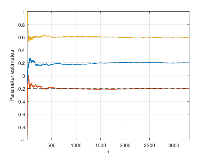
We consider a third order system with $\mu=1$ , $\sigma_{u}^{2}=1$ , $\sigma_{w}^{2}=1$ , $b_{1}=0.2$ , $b_{2}=-0.2$ , $b_{3}=0.6$ . In the plots below we will use the sequence $\alpha_{j}=\frac{10}{j}$ . An initial truncation bound of $M_{0}=1000$ was used, but was never exceeded in our simulations. We first consider the case where $\mu$ and $\sigma_{u}^{2}$ are known to the estimator. Fig. 2 shows the estimates $\hat{b}_{1},\hat{b}_{2},\hat{b}_{3}$ from Algorithm 1, and as expected from Theorem II.2, they converge to the true values.

To look at the convergence behaviour, we can approximate the variance of $j^{1/2}(\hat{b}_{n,j}-b_{n}),n=1,2,3$ [38], [37]. However, in order to allow for a fairer comparison with the algorithms of Section III, we will instead approximate the variance of $t^{1/2}(\hat{b}_{n,j}-b_{n}),n=1,2,3$ , where $t$ is the time index. This is done by computing the sample variance over 10000 different simulation runs of Algorithm 1, and are given in Fig. 3.

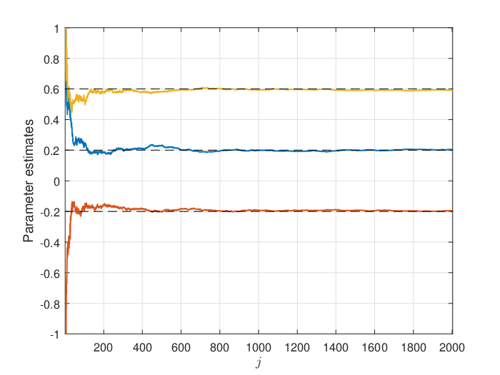
Next, we consider the system identification scheme of Section II-C where $\mu$ and $\sigma_{u}^{2}$ are not assumed to be known. Fig. 4 shows the estimates $\hat{b}_{1},\hat{b}_{2},\hat{b}_{3}$ from Algorithm 2. Also in this case, the estimates converge to the true values, in agreement with Theorem II.4.

Approximations of the variances $t^{1/2}(\hat{b}_{n,j}-b_{n}),n=1,2,3$ using Monte Carlo approximations over 10000 simulation runs are plotted in Fig. 5. We see that the normalized variances in Fig. 5 are significantly higher (more than double) than for Algorithm 1, due to the need to also estimate the parameters of the input distribution.

III Quantizers With Computational Capabilities

The setup in Section II assumes knowledge of the input and noise distributions. Specifically, we assumed that the input and noise were both Gaussian. For unknown distributions and FIR systems of order $N>1$ , it appears to be difficult to come up with an identification scheme that is consistent and/or efficient.³³ 3 For $N=1$ a consistent identification scheme was developed in [28] for symmetrically distributed inputs and noises. In this section we consider the case where the input and output quantizers are “smart”, in the sense that they have some computational and storage capabilities, and have access to the unquantized inputs and outputs. For instance, in many wireless sensor network applications such as in environmental monitoring [39, 40] and process industries [41], the sensors used often have sensing, computation and wireless communication capabilities. In such applications the quantization or analog-to-digital (A/D) conversion is done by the sensor, and additionally these sensors would also have some on-board computing capabilities to do additional processing of the data. For such situations we present in this section identification schemes which can estimate the parameters for unknown input and noise distributions.

III-A Data Generating System and Model

As in Section II, the system to be identified is an $N$ -th order FIR system

y_{t}=b_{1}u_{t-1}+b_{2}u_{t-2}+\dots+b_{N}u_{t-N}+w_{t}.

(18)

We now make the following assumptions:
Assumption 5: The input and output quantizers have computational and storage capabilities.
Assumption 6: The input sequence $\{u_{t}\}$ and the noise sequence $\{w_{t}\}$ are i.i.d. and mutually independent. Moreover, $w_{t}$ is zero mean.
Assumption 7: The model order $N$ is known.

III-B Identification Scheme for Known Input Distribution

In this subsection, we will also make the following assumption:
Assumption 8: The input distribution is known to the estimator.

The noise distribution is not assumed to be known, apart from assuming that it has zero mean. As in Section II-B, we will start by describing the ideas involved, before formally stating the identification scheme as Algorithm 3, followed by a proof of strong consistency of the parameter estimates.

First, the quantized information $\mathds{1}(u_{t}>c_{u}),t=1,2,\dots$ sent by the input quantizer to the estimator is forwarded by the estimator to the output quantizer. Whenever $u_{t}>c_{u}$ , we increment an index $i$ by one. Denote the times where $u_{t}>c_{u}$ by $\tau_{1},\tau_{2},\dots$ , with $\tau_{1}<\tau_{2}<\dots$ . The output quantizer computes the following $N$ quantities (after the corresponding output is available at the quantizer):

d_{n,i}\triangleq\frac{1}{i}\sum_{i^{\prime}=1}^{i}y_{\tau_{i^{\prime}}+n},\quad n=1,\dots,N,

using the recursions

d_{n,i}=\frac{1}{i}(y_{\tau_{i}+n}+(i-1)d_{n,i-1}),\quad n=1,\dots,N.

(19)

By the ergodic theorem [36, p. 393], we have that as $i\rightarrow\infty$ ,

\begin{split}d_{n,i}&\stackrel{{\scriptstyle\textrm{a.s.}}}{{\rightarrow}}\mathbb{E}[y_{t+n}|u_{t}>c_{u}]\\ &=\mathbb{E}\Big[\sum_{m=1}^{N}b_{m}u_{t+n-m}+n_{t+n}\Big|u_{t}>c_{u}\Big]\\ &=b_{1}\mathbb{E}[u]+\dots+b_{n-1}\mathbb{E}[u]+b_{n}\mathbb{E}[u|u>c]\\ &\quad+b_{n+1}\mathbb{E}[u]+\dots+b_{N}\mathbb{E}[u]\\ &\triangleq d_{n},\quad n=1,\dots,N.\end{split}

(20)

$d_{n,i}$ is computed at the output quantizer. In order for the estimator to be able to approximate $d_{n,i}$ , information is sent from the output quantizer to the estimator as follows. Whenever the index $i$ is a multiple of $N$ , another iteration index $j$ is incremented by one and the following estimates of $d_{1},\dots,d_{N}$ are computed at the output quantizer:

\begin{split}\hat{d}_{n,j+1}&=\hat{d}_{n,j}+\alpha_{j}\textrm{sgn}(d_{n,i}-\hat{d}_{n,j}),\quad n=1,\dots,N,\end{split}

(21)

where $\{\alpha_{j}\}$ is a sequence satisfying $\alpha_{j}>0,\sum_{j=0}^{\infty}\alpha_{j}=\infty,\sum_{j=0}^{\infty}\alpha_{j}^{2}<\infty$ , and

\textrm{sgn}(x)\triangleq\left\{\begin{array}[]{rcl}-1&,&x<0\\ 1&,&x>0.\end{array}\right.

The term $\textrm{sgn}(d_{n,i}-\hat{d}_{n,j})$ is essentially binary, and is sent to the estimator by the output quantizer, which also computes $\hat{d}_{n,j+1}$ according to (21), assuming that both the estimator and the quantizer have access to the initial condition $\hat{d}_{n,0}$ . Alternatively, $\hat{d}_{n,j}$ can be computed at the estimator only and transmitted to the output quantizer.

Note that $\hat{d}_{n,j}$ is updated at $1/N$ -th the rate of $d_{n,i}$ , in order for each of the quantities $\textrm{sgn}(d_{n,i}-\hat{d}_{n,j}),n=1,\dots,N$ to be sent in separate time slots. From (20) and (21), we can show (see the proof of Theorem III.2) that

\begin{split}\hat{d}_{n,j}\stackrel{{\scriptstyle\textrm{a.s.}}}{{\rightarrow}}d_{n}&=b_{1}\mathbb{E}[u]+\dots+b_{n-1}\mathbb{E}[u]+b_{n}\mathbb{E}[u|u>c]\\ &\quad+b_{n+1}\mathbb{E}[u]+\dots+b_{N}\mathbb{E}[u].\end{split}

(22)

Finally, the parameters $b_{1},b_{2},\dots,b_{N}$ of the $N$ -th order system (18) are estimated by solving for $\hat{b}_{1,j},\hat{b}_{2,j},\dots,\hat{b}_{N,j}$ the following set of linear equations:

\mathbf{U}\left[\hat{b}_{1,j},\dots,\hat{b}_{N,j}\right]^{T}=\left[\hat{d}_{1,j},\dots,\hat{d}_{N,j}\right]^{T},

(23)

where

\mathbf{U}\triangleq\left[\begin{array}[]{cccc}\mathbb{E}[u|u>c_{u}]&\mathbb{E}[u]&\dots&\mathbb{E}[u]\\ \mathbb{E}[u]&\mathbb{E}[u|u>c_{u}]&\dots&\mathbb{E}[u]\\ \vdots&\vdots&\ddots&\vdots\\ \mathbb{E}[u]&\mathbb{E}[u]&\dots&\mathbb{E}[u|u>c_{u}]\end{array}\right].

(24)

Note that $\mathbf{U}$ is known at the estimator, since by Assumption 8 the estimator knows the input distribution. The equations (23) will have a unique solution under the following assumption:
Assumption 9: The input distribution of $u$ and input quantizer threshold $c_{u}$ satisfies $\mathbb{E}[u|u>c_{u}]\neq\mathbb{E}[u]$ and $\mathbb{E}[u|u>c_{u}]\neq(1-N)\mathbb{E}[u]$ .

We note that apart from degenerate cases such as $u$ being constant, $c_{u}$ can always be chosen such that Assumption 9 is satisfied. Under Assumption 9, when $\mathbb{E}[u]\neq 0$ we have uniqueness of solutions to (23) by the following result:

Lemma III.1

The $N\times N$ matrix

\mathbf{A}\triangleq\left[\begin{array}[]{cccc}a&1&\dots&1\\ 1&a&\dots&1\\ \vdots&\vdots&\ddots&\vdots\\ 1&1&\dots&a\end{array}\right]

(25)

is invertible if $a\neq 1$ and $a\neq 1-N$ .

Proof:

We use the property that a matrix $\mathbf{A}$ is invertible if and only if $\mathbf{Ax}=\mathbf{0}\Rightarrow\mathbf{x}=\mathbf{0}$ . Denoting $\mathbf{x}\triangleq[x_{1},x_{2},\dots,x_{N}]^{T}$ , $\mathbf{Ax}=\mathbf{0}$ (for $\mathbf{A}$ given by (25)) is equivalent to

\begin{split}&ax_{1}+x_{2}+\dots+x_{N}=0\\ &x_{1}+ax_{2}+\dots+x_{N}=0\\ &\quad\quad\quad\vdots\\ &x_{1}+x_{2}+\dots+ax_{N}=0.\end{split}

(26)

Subtracting the second equation from the first equation in (26), we have $(x_{1}-x_{2})(a-1)=0$ , which implies that $x_{1}=x_{2}$ since $a\neq 1$ . Repeating this argument leads to

x_{1}=x_{2}=\dots=x_{N}.

(27)

Using (27) on the first equation of (26), we have $(a+N-1)x_{1}=0$ , which implies $x_{1}=0$ since $a\neq 1-N$ . Hence $\mathbf{x}=\mathbf{0}$ . ∎

We now formally state the identification scheme as Algorithm 3. In the formal description, the sets $\mathcal{D}_{t}$ and indices $i_{n}$ are used to keep track of which of the quantities $d_{n,i},\ n=1,\ldots,N$ , should be updated at time $t$ .

Algorithm 3 • Choose a $c_{u}$ satisfying Assumption 9, and a sequence $\{\alpha_{j}\}$ satisfying $\alpha_{j}>0$ , $\sum_{j=0}^{\infty}\alpha_{j}=\infty$ , and $\sum_{j=0}^{\infty}\alpha_{j}^{2}<\infty$ • Initialize $i=0,j=0$ , $d_{n,0}=0,\hat{d}_{n,0}=0,i_{n}=1,n=1,\dots,N,\quad\mathcal{D}_{t}=\emptyset,\forall t$ • For $t=1,2,\dots$ , do: – If $u_{t}>c_{u}$ , set $\tau_{i}=t$ , $i:=i+1$ – If $i\equiv 0\textrm{ (mod }N)$ , set $j:=j+1$ – At the input quantizer: 1. Send $\mathds{1}(u_{t}>c_{u})$ to estimator, which passes it on to the output quantizer – At the output quantizer, when $u_{t}>c_{u}$ : 1. Set $\mathcal{D}_{t+n}:=\mathcal{D}_{t+n}\bigcup\{n\},n=1,\dots,N$ 2. Compute $d_{n,i_{n}}=\frac{1}{i_{n}}(y_{t}+(i_{n}-1)d_{n,i_{n}-1})$ and set $i_{n}:=i_{n}+1$ for all $n\in\mathcal{D}_{t}$ , and remove $\mathcal{D}_{t-1}$ from memory 3. When $i\equiv 0\textrm{ (mod }N)$ , compute $\textrm{sgn}(d_{n,i}-\hat{d}_{n,j})$ and $\hat{d}_{n,j+1}=\hat{d}_{n,j}+\alpha_{j}\textrm{sgn}(d_{n,i}-\hat{d}_{n,j})$ at time $\tau_{i}+n$ for $n=1,\dots,N$ . Send $\textrm{sgn}(d_{n,i}-\hat{d}_{n,j})$ at time $\tau_{i}+n$ to estimator, for $n=1,\dots,N$ – At the estimator, when $i\equiv 0\textrm{ (mod }N)$ : 1. Compute $\left[\hat{b}_{1,j},\dots,\hat{b}_{N,j}\right]^{T}=\mathbf{U}^{-1}\left[\hat{d}_{1,j},\dots,\hat{d}_{N,j}\right]^{T}$ , where $\mathbf{U}$ is defined by (24) 2. Compute $\hat{d}_{n,j+1}=\hat{d}_{n,j}+\alpha_{j}\textrm{sgn}(d_{n,i}-\hat{d}_{n,j})$ when $\textrm{sgn}(d_{n,i}-\hat{d}_{n,j})$ arrives at estimator, for $n=1,\dots,N$

Theorem III.2

Under Algorithm 3 and Assumptions $5-9$ , $\hat{b}_{n,j}\stackrel{{\scriptstyle\textrm{a.s.}}}{{\rightarrow}}b_{n}$ as $j\rightarrow\infty$ for $n=1,\dots,N$ .

Proof:

See Appendix -E. ∎

III-C Unknown Input Distribution

Solving the linear equations (23) requires knowledge of $\mathbb{E}[u]$ and $\mathbb{E}[u|u>c_{u}]$ , which in turn requires knowledge of the distribution of $u$ . When the input distribution is unknown (except for enough knowledge such that Assumption 9 can be satisfied), $\mathbb{E}[u]$ and $\mathbb{E}[u|u>c_{u}]$ can be estimated if we also allow for some computation at the input quantizer.

To estimate $\mathbb{E}[u]$ , the input quantizer first computes

e_{1,t}\triangleq\frac{1}{t}\sum_{t^{\prime}=1}^{t}u_{t^{\prime}}

using the recursion

e_{1,t}=\frac{1}{t}(u_{t}+(t-1)e_{1,t-1}).

By the strong law of large numbers, $e_{1,t}\stackrel{{\scriptstyle\textrm{a.s.}}}{{\rightarrow}}\mathbb{E}[u]$ as $t\rightarrow\infty$ . The estimator estimates $e_{1,t}$ using the recursion:

\hat{e}_{1,j+1}=\hat{e}_{1,j}+\alpha_{j}\textrm{sgn}(e_{1,t}-\hat{e}_{1,j})

where the quantities $\textrm{sgn}(e_{1,t}-\hat{e}_{1,j})$ are sent by the input quantizer (see below for how the index $j$ is updated). Again, $\{\hat{e}_{1,j}\}$ can be reconstructed at the input quantizer given knowledge of the initial condition $\hat{e}_{1,0}$ .

To estimate $\mathbb{E}[u|u>c_{u}]$ , whenever $u_{t}>c_{u}$ , the input quantizer first increments an index $k$ by one. Denote the times when $u_{t}>c_{u}$ by $t_{1},t_{2},\dots$ , with $t_{1}<t_{2}<\dots$ . The input quantizer then computes

e_{2,k}\triangleq\frac{1}{k}\sum_{k^{\prime}=1}^{k}u_{t_{k^{\prime}}}

using the recursion

e_{2,k}=\frac{1}{k}(u_{t_{k}}+(k-1)e_{2,k-1}).

We have $e_{2,k}\stackrel{{\scriptstyle\textrm{a.s.}}}{{\rightarrow}}\mathbb{E}[u|u>c_{u}]$ as $k\rightarrow\infty$ by the strong law of large numbers. The estimator estimates $e_{2,k}$ using the recursion:

\hat{e}_{2,j+1}=\hat{e}_{2,j}+\alpha_{j}\textrm{sgn}(e_{2,k}-\hat{e}_{2,j})

where the quantities $\textrm{sgn}(e_{2,k}-\hat{e}_{2,j})$ are sent by the input quantizer.

Now in Algorithm 3, the input quantizer is already sending $\mathds{1}(u_{t}>c_{u})$ to the estimator at every time slot. Thus we need to modify the division of the time slots to incorporate the sending of the additional information $\textrm{sgn}(e_{1,t}-\hat{e}_{1,j})$ and $\textrm{sgn}(e_{2,k}-\hat{e}_{2,j})$ . We propose the following: Instead of an iteration $j$ having a (minimum) length of $N$ time slots as in Algorithm 3, we will now consider iterations $j$ with a (minimum) length of $N+2$ time slots. During the first $N$ time slots, the input quantizer will send $\mathds{1}(u_{t}>c_{u})$ to the estimator, which are then forwarded to the output quantizer. As in Algorithm 3, an index $i$ is now incremented by one⁴⁴ 4 The indices $i$ and $k$ are different, as in the updating of $k$ one checks if $u_{t}>c_{u}$ at every time step, to obtain more accurate estimates. every time $u_{t}>c_{u}$ (during the first $N$ time slots), and the iteration index $j$ is incremented by one whenever $i$ is a multiple of $N$ . The remaining two time slots will be used to transmit the quantities $\textrm{sgn}(e_{1,t}-\hat{e}_{1,j})$ and $\textrm{sgn}(e_{2,k}-\hat{e}_{2,j})$ .

The parameters $b_{1},b_{2},\dots,b_{N}$ are now estimated by solving for $\hat{b}_{1,j},\hat{b}_{2,j},\dots,\hat{b}_{N,j}$ the following set of linear equations:

\mathbf{U}_{j}\left[\hat{b}_{1,j},\dots,\hat{b}_{N,j}\right]^{T}=\left[\hat{d}_{1,j},\dots,\hat{d}_{N,j}\right]^{T}

(28)

where

\mathbf{U}_{j}\triangleq\left[\begin{array}[]{cccc}\hat{e}_{2,j}&\hat{e}_{1,j}&\dots&\hat{e}_{1,j}\\ \hat{e}_{1,j}&\hat{e}_{2,j}&\dots&\hat{e}_{1,j}\\ \vdots&\vdots&\ddots&\vdots\\ \hat{e}_{1,j}&\hat{e}_{1,j}&\dots&\hat{e}_{2,j}\end{array}\right].

(29)

The formal statement of the identification scheme is given as Algorithm 4.

Algorithm 4 • Choose a $c_{u}$ satisfying Assumption 9, and a sequence $\{\alpha_{j}\}$ satisfying $\alpha_{j}>0$ , $\sum_{j=0}^{\infty}\alpha_{j}=\infty$ , and $\sum_{j=0}^{\infty}\alpha_{j}^{2}<\infty$ . • Initialize $i=0,j=0,k=0$ , $d_{n,0}=0,\hat{d}_{n,0}=0,i_{n}=1,n=1,\dots,N$ , $e_{1,0}=0,e_{2,0}=0$ , $\hat{e}_{1,0}=0,\hat{e}_{2,0}=0$ , $\mathcal{D}_{t}=\emptyset,\forall t$ • For $t=1,2,\dots$ , do: – If $u_{t}>c_{u}$ , set $t_{k}=t$ , $k:=k+1$ – If $t\textrm{ mod }(N+2)\in\{1,\dots,N\}$ and $u_{t}>c_{u}$ , set $\tau_{i}=t$ , $i:=i+1$ – If $i\equiv 0\textrm{ (mod }N)$ , set $j:=j+1$ – At the input quantizer: 1. Compute $e_{1,t}=\frac{1}{t}(u_{t}+(t-1)e_{1,t-1})$ and $e_{2,k}=\frac{1}{k}(u_{t_{k}}+(k-1)e_{2,k-1})$ 2. Send $\mathds{1}(u_{t}>c_{u})$ to estimator if $t\textrm{ mod }(N+2)\in\{1,\dots,N\}$ , which passes it on to the output quantizer 3. When $i\equiv 0\textrm{ (mod }N)$ , compute $\textrm{sgn}(e_{1,t}-\hat{e}_{1,j})$ , $\textrm{sgn}(e_{2,k}-\hat{e}_{2,j})$ , $\hat{e}_{1,j+1}=\hat{e}_{1,j}+\alpha_{j}\textrm{sgn}(e_{1,t}-\hat{e}_{1,j})$ , and $\hat{e}_{2,j+1}=\hat{e}_{2,j}+\alpha_{j}\textrm{sgn}(e_{2,k}-\hat{e}_{2,j})$ . Send $\textrm{sgn}(e_{1,t}-\hat{e}_{1,j})$ and $\textrm{sgn}(e_{2,k}-\hat{e}_{2,j})$ to estimator at times $\tau_{i}+N+1$ and $\tau_{i}+N+2$ respectively – At the output quantizer, when $t\textrm{ mod }(N+2)\in\{1,\dots,N\}$ and $u_{t}>c_{u}$ : 1. Set $\mathcal{D}_{t+n}:=\mathcal{D}_{t+n}\bigcup\{n\},n=1,\dots,N$ 2. Compute $d_{n,i_{n}}=\frac{1}{i_{n}}(y_{t}+(i_{n}-1)d_{n,i_{n}-1})$ and set $i_{n}:=i_{n}+1$ for all $n\in\mathcal{D}_{t}$ , and remove $\mathcal{D}_{t-1}$ from memory 3. When $i\equiv 0\textrm{ (mod }N)$ , compute $\textrm{sgn}(d_{n,i}-\hat{d}_{n,j})$ and $\hat{d}_{n,j+1}=\hat{d}_{n,i}+\alpha_{j}\textrm{sgn}(d_{n,i}-\hat{d}_{n,j})$ at time $\tau_{i}+n$ , for $n=1,\dots,N$ . Send $\textrm{sgn}(d_{n,i}-\hat{d}_{n,j})$ at time $\tau_{i}+n$ to estimator, for $n=1,\dots,N$ – At the estimator, when $i\equiv 0\textrm{ (mod }N)$ : 1. Compute $\left[\hat{b}_{1,j},\dots,\hat{b}_{N,j}\right]^{T}=\left\{\begin{array}[]{ccl}\mathbf{U}_{j}^{-1}\left[\hat{d}_{1,j},\dots,\hat{d}_{N,j}\right]^{T}&,&\textrm{if }\mathbf{U}_{j}\textrm{ is invertible}\\ 0&,&\textrm{otherwise}\end{array}\right.$ where $\mathbf{U}_{j}$ is defined by (29) 2. Compute $\hat{d}_{n,j+1}=\hat{d}_{n,i}+\alpha_{j}\textrm{sgn}(d_{n,i}-\hat{d}_{n,j}),n=1,\dots,N$ , $\hat{e}_{1,j+1}=\hat{e}_{1,j}+\alpha_{j}\textrm{sgn}(e_{1,t}-\hat{e}_{1,j})$ , and $\hat{e}_{2,j+1}=\hat{e}_{2,j}+\alpha_{j}\textrm{sgn}(e_{2,k}-\hat{e}_{2,j})$ , when the quantities $\textrm{sgn}(d_{n,i}-\hat{d}_{n,j})$ , $\textrm{sgn}(e_{1,t}-\hat{e}_{1,j})$ , $\textrm{sgn}(e_{2,k}-\hat{e}_{2,j})$ arrive at estimator

Theorem III.3

Under Algorithm 4 and Assumptions $5,6,7,9$ , $\hat{b}_{n,j}\stackrel{{\scriptstyle\textrm{a.s.}}}{{\rightarrow}}b_{n}$ as $j\rightarrow\infty$ for $n=1,\dots,N$ .

Proof:

Using similar arguments as in the proof of Theorem III.2, we can show that

\begin{split}\hat{d}_{n,j}&\stackrel{{\scriptstyle\textrm{a.s.}}}{{\rightarrow}}b_{1}\mathbb{E}[u]+\dots+b_{n-1}\mathbb{E}[u]+b_{n}\mathbb{E}[u|u>c_{u}]\\ &\qquad+b_{n+1}\mathbb{E}[u]+\dots+b_{N}\mathbb{E}[u],\quad n=1,\dots,N,\\ \hat{e}_{1,j}&\stackrel{{\scriptstyle\textrm{a.s.}}}{{\rightarrow}}\mathbb{E}[u],\textrm{ and }\hat{e}_{2,j}\stackrel{{\scriptstyle\textrm{a.s.}}}{{\rightarrow}}\mathbb{E}[u|u>c_{u}].\end{split}

(30)

Hence by (30) and continuity,

\begin{split}\left[\hat{b}_{1,j},\dots,\hat{b}_{N,j}\right]^{T}&=\mathbf{U}_{j}^{-1}\left[\hat{d}_{1,j},\dots,\hat{d}_{N,j}\right]^{T}\\ &\stackrel{{\scriptstyle\textrm{a.s.}}}{{\rightarrow}}\mathbf{U}^{-1}\mathbf{U}\left[b_{1},\dots,b_{N}\right]^{T}=\left[b_{1},\dots,b_{N}\right]^{T}.\end{split}

∎

III-D Simulation Results

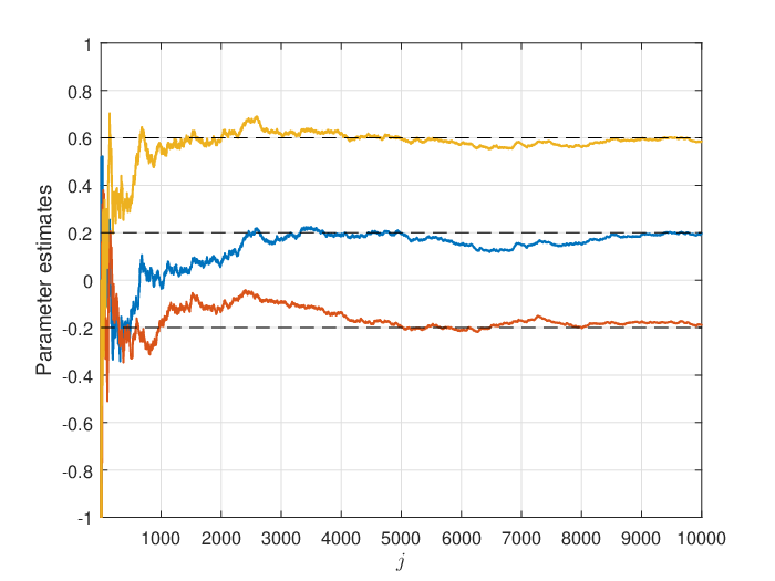
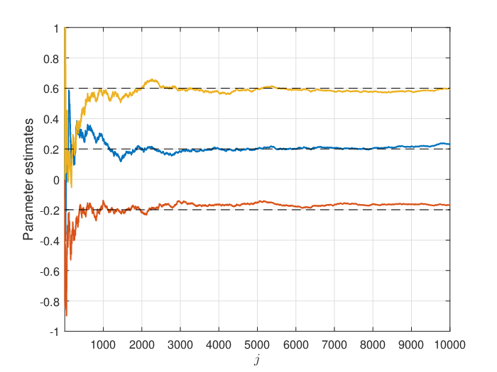
We first consider the same third order system as in Section II-D, where $b_{1}=0.2$ , $b_{2}=-0.2$ , $b_{3}=0.6$ , and the inputs and noises are Gaussian with $\mu=1$ , $\sigma_{u}^{2}=1$ , $\sigma_{w}^{2}=1$ . We use the identification schemes in Algorithms 3 and 4. In the schemes we use the sequences $\alpha_{j}=\frac{1}{j}$ , and the threshold $c_{u}=1$ . Figs. 6 and 7 shows the estimates $\hat{b}_{1},\hat{b}_{2},\hat{b}_{3}$ from Algorithms 3 and 4 respectively.

Next, we change $w_{t}$ to be uniformly distributed between $-\sqrt{3}$ and $\sqrt{3}$ , and $u_{t}$ to be uniformly distributed between $0$ and $2\sqrt{3}$ (so that the variances are equal to 1). Fig. 8 shows the estimates $\hat{b}_{1},\hat{b}_{2},\hat{b}_{3}$ from Algorithm 4.

Approximations of the variances $t^{1/2}(\hat{b}_{n,j}-b_{n}),n=1,2,3$ using Monte Carlo approximations over 10000 simulation runs are plotted for the Gaussian distributed inputs and noise case with Algorithms 3 and 4 in Figs. 9 and 10 respectively, and for uniformly distributed inputs and noise in Fig. 11. Comparing Figs. 9 and 10 with Figs. 3 and 5, we see that the normalized variances are much smaller, and hence convergence of the algorithms is better, when the quantizers have some computational and storage capabilities. We do emphasize however that the algorithms are based on different principles, so it is not a straightforward comparison.

TABLE I: Summary of identification algorithms

Algorithm	Computational Capability	Input Signal	Output Noise	Input Parameter
	of Quantizer			Knowledge
Algorithm 1	None	i.i.d. Gaussian	i.i.d. zero-mean Gaussian	$(\mu,\sigma_{u}^{2})$
Algorithm 2	None	i.i.d. Gaussian	i.i.d. zero-mean Gaussian	None
Algorithm 3	At output quantizer	i.i.d.	i.i.d. zero-mean	$\mathbb{E}[u]$ & $\mathbb{E}[u\|u>c_{u}]$
Algorithm 4	At input & output quantizers	i.i.d.	i.i.d. zero-mean	None

IV Conclusion

This paper has considered the identification of FIR systems with binary input and output observations. For the case where the quantizer thresholds can be adapted but the quantizers have no computational capabilities, we proposed identification schemes which are strongly consistent for Gaussian distributed inputs and noises. For the case of smart quantizers which have some computational and storage capabilities, strongly consistent identification schemes are proposed which can handle arbitrary input and noise distributions. A summary of the main features and assumptions required for the different algorithms is provided in Table I. Numerical simulations have illustrated the performance of the algorithms. Rigorous analyses of the convergence rates of the algorithms is currently under investigation.

-A Proof of Lemma II.1

First note that

		$\displaystyle\frac{\partial}{\partial b}\Bigg[1-\Phi\Bigg(\frac{-b(u-\mu)}{\sqrt{\widehat{\textrm{V}y}-b^{2}\sigma_{u}^{2}}}\Bigg)\Bigg]=\frac{1}{\sqrt{2\pi}}\exp\left(-\frac{b^{2}(u-\mu)^{2}}{2(\widehat{\textrm{V}y}-b^{2}\sigma_{u}^{2})}\right)$
		$\displaystyle\quad\times\left[\frac{b^{2}\sigma_{u}^{2}(u-\mu)}{(\widehat{\textrm{V}y}-b^{2}\sigma_{u}^{2})^{3/2}}+\frac{u-\mu}{(\widehat{\textrm{V}y}-b^{2}\sigma_{u}^{2})^{1/2}}\right]$

is continuous for $b\in\Big(-\sqrt{\widehat{\textrm{V}y}/\sigma_{u}^{2}},\sqrt{\widehat{\textrm{V}y}/\sigma_{u}^{2}}\Big)$ , since quotients and compositions of continuous functions are continuous. For fixed $\widehat{\textrm{V}y}$ , regard $F(b,\widehat{\textrm{V}y})$ as a function of $b$ . Then by the Leibniz rule, we have that

\begin{split}\frac{dF}{db}&=\int_{\mu}^{\infty}\frac{\partial}{\partial b}\Bigg[1-\Phi\Bigg(\frac{-b(u-\mu)}{\sqrt{\widehat{\textrm{V}y}-b^{2}\sigma_{u}^{2}}}\Bigg)\Bigg]p(u)du\\ &=\int_{\mu}^{\infty}\frac{1}{\sqrt{2\pi}}\exp\left(-\frac{b^{2}(u-\mu)^{2}}{2(\widehat{\textrm{V}y}-b^{2}\sigma_{u}^{2})}\right)\\ &\quad\times\left[\frac{b^{2}\sigma_{u}^{2}(u-\mu)}{(\widehat{\textrm{V}y}-b^{2}\sigma_{u}^{2})^{3/2}}+\frac{u-\mu}{(\widehat{\textrm{V}y}-b^{2}\sigma_{u}^{2})^{1/2}}\right]p(u)du\\ &>0,\quad\forall b\in\left(-\sqrt{\widehat{\textrm{V}y}/\sigma_{u}^{2}},\sqrt{\widehat{\textrm{V}y}/\sigma_{u}^{2}}\right),\end{split}

since each term in the integrand is strictly positive for $b\in\Big(-\sqrt{\widehat{\textrm{V}y}/\sigma_{u}^{2}},\sqrt{\widehat{\textrm{V}y}/\sigma_{u}^{2}}\Big)$ and $u>\mu$ .

-B Statement of Theorem 2.4.1(ii) of [38]

We provide here the statement of Theorem 2.4.1(ii) of [38], adapted to the notation of this paper. A major part of the proof of Theorem II.2 is the verification of the conditions of this theorem.

Theorem .1 (Theorem 2.4.1(ii) of [38])

Consider the procedure

x_{j+1}=\Pi_{M_{\varsigma(j)}}(x_{j}+\alpha_{j}(f(x_{j})+\varepsilon_{j}))

where

\varsigma(0)=0,\quad\varsigma(j)\triangleq\sum_{i=1}^{j-1}\mathds{1}(||x_{i}+\alpha_{i}(f(x_{i})+\varepsilon_{i})||>M_{\varsigma(i)}),

and the truncation operation

\Pi_{M}(x)\triangleq\left\{\begin{array}[]{ll}x,&||x||\leq M\\ x^{*},&||x||>M.\end{array}\right.

Suppose $f(.):\mathbb{R}^{l}\rightarrow\mathbb{R}$ has a unique root $x^{0}$ , and $f(.)$ is continuous at $x^{0}$ . Further assume that conditions A2.2.1 and A2.2.2 below hold.
A2.2.1: $\alpha_{j}>0$ , $\alpha_{j}\rightarrow 0$ , and $\sum_{j=1}^{\infty}\alpha_{j}=\infty$ .
A2.2.2: There exists a continuously differentiable function $v(.):\mathbb{R}^{l}\rightarrow\mathbb{R}$ such that

\sup_{\delta\leq||x-x^{0}||\leq\Delta}f^{T}(x)\nabla v(x)<0

(31)

for any $\Delta>\delta>0$ , and

v(x^{*})<\inf_{||x||=c_{0}}v(x)

(32)

for some $c_{0}>0$ and $||x^{*}||<c_{0}$ .

Then $\{x_{j}\}$ converges to $x^{0}$ for those sample paths where $\varepsilon_{j}$ can be written as $\varepsilon_{j}=\varepsilon_{j}^{(1)}+\varepsilon_{j}^{(2)}$ , with

\sum_{j=1}^{\infty}\alpha_{j}\varepsilon_{j}^{(1)}<\infty\textrm{ and }\varepsilon_{j}^{(2)}\rightarrow 0.

-C Proof of Theorem II.2

The idea of the proof is that we will first show that Algorithm 1 can be viewed as a multi-dimensional stochastic approximation algorithm with expanding truncations. We will then verify the conditions of Theorem 2.4.1(ii) of [38] (given in Appendix -B) to conclude that $\hat{b}_{n,j}\stackrel{{\scriptstyle\textrm{a.s.}}}{{\rightarrow}}b_{n}$ as $j\rightarrow\infty$ for $n=1,\dots,N$ .

Define $f(.):\mathbb{R}^{N+2}\rightarrow\mathbb{R}^{N+2}$ by

f\left(\!\left[\begin{array}[]{c}c_{y}\\ \tilde{c}_{y}\\ \hat{b}_{1}\\ \vdots\\ \hat{b}_{N}\end{array}\right]\!\right)\triangleq\left[\!\!\begin{array}[]{c}\mathbb{P}(y_{t}>c_{y})-0.5\\ \mathbb{P}(y_{t}>\tilde{c}_{y})-0.1587\\ F(b_{1},(\tilde{c}_{y}-c_{y})^{2})-F(\hat{b}_{1},(\tilde{c}_{y}-c_{y})^{2})\\ \vdots\\ F(b_{N},(\tilde{c}_{y}-c_{y})^{2})-F(\hat{b}_{N},(\tilde{c}_{y}-c_{y})^{2})\end{array}\!\!\right].

where

\mathbb{P}(y_{t}>c)=1-\Phi\bigg(\frac{c-(b_{1}+\dots+b_{N})\mu}{\sqrt{(b_{1}^{2}+\dots+b_{N}^{2})\sigma_{u}^{2}+\sigma_{w}^{2}}}\bigg)

is the stationary probability that $y_{t}>c$ , and $F(.,.)$ is given by (6).

Since $y_{t}$ is Gaussian, the unique solution to $\mathbb{P}(y_{t}>c_{y})-0.5=0$ is clearly $c_{y}=\mathbb{E}[y]$ , and the unique solution to $\mathbb{P}(y_{t}>\tilde{c}_{y})-0.1587=0$ is clearly $\tilde{c}_{y}=\mathbb{E}[y]+\sqrt{\textrm{Var}[y]}$ . For $c_{y}=\mathbb{E}[y]$ and $\tilde{c}_{y}=\mathbb{E}[y]+\sqrt{\textrm{Var}[y]}$ , each of the equations

F(b_{n},(\tilde{c}_{y}-c_{y})^{2})-F(\hat{b}_{n},(\tilde{c}_{y}-c_{y})^{2})=0

has the unique solution $\hat{b}_{n}=b_{n}$ (i.e. the true value of the parameter) by Lemma II.1. Hence the equation

f([c_{y},\tilde{c}_{y},\hat{b}_{1},\dots,\hat{b}_{N}]^{T})=\mathbf{0}

(33)

has the unique root

[c_{y},\tilde{c}_{y},\hat{b}_{1},\dots,\hat{b}_{N}]^{T}\!=\![\mathbb{E}[y],\mathbb{E}[y]+\sqrt{\textrm{Var}[y]},b_{1},\dots,b_{N}]^{T}\!\triangleq\!x^{0}.

(34)

Next, let us write the recursions in Algorithm 1 in the following form:

\begin{split}&\left[\!\!\!\begin{array}[]{c}c_{y,j+1}\\ \tilde{c}_{y,j+1}\\ \hat{b}_{1,j+1}\\ \vdots\\ \hat{b}_{N,j+1}\end{array}\!\!\!\right]=\Pi_{M_{\varsigma(j)}}\left(\left[\!\!\!\begin{array}[]{c}c_{y,j}\\ \tilde{c}_{y,j}\\ \hat{b}_{1,j}\\ \vdots\\ \hat{b}_{N,j}\end{array}\!\!\!\right]+\alpha_{j}f\left(\!\left[\!\!\begin{array}[]{c}c_{y,j}\\ \tilde{c}_{y,j}\\ \hat{b}_{1,j}\\ \vdots\\ \hat{b}_{N,j}\end{array}\!\!\right]\!\right)+\alpha_{j}\varepsilon_{j}\right)\end{split}

(35)

where

\begin{split}&\varepsilon_{j}\triangleq\\ &\left[\!\!\begin{array}[]{c}\mathds{1}(y_{2j-1}>c_{y,j})-\mathbb{P}(y_{t}>c_{y,j})\\ \mathds{1}(y_{2j}>\tilde{c}_{y,j})-\mathbb{P}(y_{t}>\tilde{c}_{y,j})\\ \mathds{1}(u_{2j-2}>\mu)\mathds{1}(y_{2j-1}>c_{y,j})-F(b_{1},(\tilde{c}_{y,j}-c_{y,j})^{2})\\ \vdots\\ \mathds{1}(u_{2j-1-N}\!>\!\mu)\mathds{1}(y_{2j-1}\!>\!c_{y,j})-F(b_{N},(\tilde{c}_{y,j}\!-\!c_{y,j})^{2})\end{array}\!\!\right],\end{split}

(36)

which is in the form of a multi-dimensional stochastic approximation algorithm, that tries to find the roots of the equation (33), with the “noise” term being $\varepsilon_{j}$ .

We will now verify the conditions of Theorem 2.4.1(ii) of [38], whose statement is also given in Appendix -B. We first need $f(.)$ to have a unique root $x^{0}$ , with $f(.)$ continuous at $x^{0}$ . Uniqueness of $x^{0}$ given by (34) has been shown at the beginning of the proof, and $f(.)$ is clearly continuous at $x^{0}$ .

Note that Condition A2.2.1 is true by assumption. We next verify Condition A2.2.2. Choose $v(x)\triangleq||x-x^{0}||^{2}$ , i.e.

v\left([c_{y},\tilde{c}_{y},\hat{b}_{1},\dots,\hat{b}_{N}]^{T}\right)=\left\|[c_{y},\tilde{c}_{y},\hat{b}_{1},\dots,\hat{b}_{N}]^{T}-x_{0}\right\|^{2}.

Then

\begin{split}&f^{T}\left([c_{y},\tilde{c}_{y},\hat{b}_{1},\dots,\hat{b}_{N}]^{T}\right)\nabla v_{n}\left([c_{y},\tilde{c}_{y},\hat{b}_{1},\dots,\hat{b}_{N}]^{T}\right)\\ &=2\left[\begin{array}[]{c}\mathbb{P}(y_{t}>c_{y})-0.5\\ \mathbb{P}(y_{t}>\tilde{c}_{y})-0.1587\\ F(b_{1},(\tilde{c}_{y}-c_{y})^{2})-F(\hat{b}_{1},(\tilde{c}_{y}-c_{y})^{2})\\ \vdots\\ F(b_{N},(\tilde{c}_{y}-c_{y})^{2})-F(\hat{b}_{N},(\tilde{c}_{y}-c_{y})^{2})\end{array}\right]^{T}\\ &\qquad\qquad\times\left([c_{y},\tilde{c}_{y},\hat{b}_{1},\dots,\hat{b}_{N}]^{T}-x_{0}\right)\\ &<0,\,\,\forall[c_{y},\tilde{c}_{y},\hat{b}_{1},\dots,\hat{b}_{N}]^{T}\neq x^{0}.\end{split}

The inequality above holds since $\mathbb{P}(y_{t}>c_{y})-0.5$ and $\mathbb{P}(y_{t}>\tilde{c}_{y})-0.1587$ are strictly decreasing in $c_{y}$ and $\tilde{c}_{y}$ respectively,

F(b_{n},(\tilde{c}_{y}-c_{y})^{2})-F(\hat{b}_{n},(\tilde{c}_{y}-c_{y})^{2})

for fixed $c_{y}$ and $\tilde{c}_{y}$ is decreasing in $\hat{b}_{n},n=1,\dots,N$ by Lemma II.1, and for $c_{y}=\mathbb{E}[y]$ and $\tilde{c}_{y}=\mathbb{E}[y]+\sqrt{\textrm{Var}[y]}$ only takes on the value 0 when $\hat{b}_{n}=b_{n}$ . This verifies (31). Also, by the reverse triangle inequality, we have

v(x)=||x-x^{0}||^{2}\geq\Big|||x||-||x^{0}||\Big|^{2}

so that for some $c_{0}>2||x^{0}||$ , one has

\inf_{||x||=c_{0}}v(x)>(2||x^{0}||-||x^{0}||)^{2}=||x^{0}||^{2}=v(\mathbf{0}).

By our choice of $x^{*}=\mathbf{0}$ , this verifies (32) and hence condition A2.2.2.

Finally, we want to show that $\varepsilon_{j}$ can be written as $\varepsilon_{j}=\varepsilon_{j}^{(1)}+\varepsilon_{j}^{(2)}$ , with

\sum_{j=1}^{\infty}\alpha_{j}\varepsilon_{j}^{(1)}<\infty\textrm{ a.s. and }\varepsilon_{j}^{(2)}\rightarrow 0\textrm{ a.s.},

which will then imply the a.s. convergence of $[c_{y,j},\tilde{c}_{y,j},\hat{b}_{1,j},\dots,\hat{b}_{N,j}]^{T}$ to $x^{0}$ . Rewrite (36) as

\begin{split}&\varepsilon_{j}=\\ &\left[\begin{array}[]{l}\mathds{1}(y_{2j-1}>c_{y,j})-\mathbb{P}(y_{2j-1}>c_{y,j})\\ \mathds{1}(y_{2j}>\tilde{c}_{y,j})-\mathbb{P}(y_{2j}>\tilde{c}_{y,j})\\ \mathds{1}(u_{2j-2}>\mu)\mathds{1}(y_{2j-1}>c_{y,j})\\ \qquad-\mathbb{P}(u_{2j-2}>\mu,y_{2j-1}>c_{y,j})\\ \qquad\qquad\vdots\\ \mathds{1}(u_{2j-1-N}>\mu)\mathds{1}(y_{2j-1}>c_{y,j})\\ \qquad-\mathbb{P}(u_{2j-1-N}>\mu,y_{2j-1}>c_{y,j})\end{array}\right]+\\ &\left[\!\!\begin{array}[]{l}\mathbb{P}(y_{2j-1}>c_{y,j})-\mathbb{P}(y_{t}>c_{y,j})\\ \mathbb{P}(y_{2j}>\tilde{c}_{y,j})-\mathbb{P}(y_{t}>\tilde{c}_{y,j})\\ \mathbb{P}(u_{2j-2}>\mu,y_{2j-1}>c_{y,j})-\mathbb{P}(u_{t-1}>\mu,y_{t}>c_{y,j})\\ \qquad+\mathbb{P}(u_{t-1}>\mu,y_{t}>c_{y,j})-F(b_{1},(\tilde{c}_{y,j}-c_{y,j})^{2})\\ \qquad\qquad\vdots\\ \mathbb{P}(u_{2j-1-N}>\mu,y_{2j-1}>c_{y,j})-\mathbb{P}(u_{t-N}>\mu,y_{t}>c_{y,j})\\ \qquad+\mathbb{P}(u_{t-N}>\mu,y_{t}>c_{y,j})-F(b_{N},(\tilde{c}_{y,j}-c_{y,j})^{2})\end{array}\!\!\right]\\ &\triangleq\left[\varepsilon_{j}^{(1,1)},\varepsilon_{j}^{(2,1)},\varepsilon_{j}^{(3,1)},\dots,\varepsilon_{j}^{(N+2,1)}\right]^{T}\\ &\quad+\left[\varepsilon_{j}^{(1,2)},\varepsilon_{j}^{(2,2)},\varepsilon_{j}^{(3,2)},\dots,\varepsilon_{j}^{(N+2,2)}\right]^{T}.\end{split}

We will prove that $\sum_{j=1}^{\infty}\alpha_{j}\varepsilon_{j}^{(i,1)}<\infty\textrm{ a.s.}$ and $\varepsilon_{j}^{(i,2)}\stackrel{{\scriptstyle\textrm{a.s.}}}{{\rightarrow}}0$ for $i=1,2,\dots,N+2$ .

In order to show that $\sum_{j=1}^{\infty}\alpha_{j}\varepsilon_{j}^{(i,1)}<\infty\textrm{ a.s.}$ , we will show that each $\{\varepsilon_{j}^{(i,1)}\}$ is a martingale difference sequence, which will then imply that $\sum_{j=1}^{\infty}\alpha_{j}\varepsilon_{j}^{(i,1)}<\infty\textrm{ a.s.}$ , by e.g. Theorem B.6.1 of [38]. Define the $\sigma$ -algebras

\begin{split}&\mathcal{F}_{j}\triangleq\sigma\big(\{\mathds{1}(y_{2i-1}>c_{y,i}),\mathds{1}(y_{2i}>\tilde{c}_{y,i}),\mathds{1}(u_{2i-2}>\mu),\\ &\qquad\qquad i=1,\dots,j\}\big).\end{split}

(37)

From the recursion for $c_{y,j}$ , we note that $c_{y,j}$ is measurable with respect to $\mathcal{F}_{j}$ (and in fact is also measurable with respect to $\mathcal{F}_{j-1}$ ), and so $\varepsilon_{j}^{(1,1)}$ is measurable with respect to $\mathcal{F}_{j}$ . We have

\begin{split}\mathbb{E}[\varepsilon_{j}^{(1,1)}|\mathcal{F}_{j-1}]&=\mathbb{E}[\mathds{1}(y_{2j-1}>c_{y,j})-\mathbb{P}(y_{2j-1}>c_{y,j})|\mathcal{F}_{j-1}]\\ &=0.\end{split}

Thus $\{\varepsilon_{j}^{(1,1)}\}$ is a martingale difference sequence. Similar arguments can be used to show that $\{\varepsilon_{j}^{(i,1)}\}$ for $i=2,\dots,N+2$ are martingale difference sequences, and therefore that $\sum_{j=1}^{\infty}\alpha_{j}\varepsilon_{j}^{(i,1)}<\infty\textrm{ a.s.}$

Let us now show that $\varepsilon_{j}^{(1,2)}=\mathbb{P}(y_{2j-1}>c_{y,j})-\mathbb{P}(y_{t}>c_{y,j})\stackrel{{\scriptstyle\textrm{a.s.}}}{{\rightarrow}}0$ . First, we note that $y_{2j-1}$ and $c_{y,j-L}$ are independent for sufficiently large $L$ , e.g. $L=N$ , so that we can write

\mathbb{P}(y_{2j-1}>c_{y,j-L})=\mathbb{P}(y_{t}>c_{y,j-L}).

(38)

Next, we note that $c_{y,j+1}$ differs from $c_{y,j}$ by $\alpha_{j}/2$ (either above or below). Since by assumption $\alpha_{j}>0,\forall j$ , we can bound the difference between $c_{y,j}$ and $c_{y,j-L}$ as follows:

c_{y,j-L}-\sum_{i=j-L}^{j-1}\frac{\alpha_{i}}{2}\leq c_{y,j}\leq c_{y,j-L}+\sum_{i=j-L}^{j-1}\frac{\alpha_{i}}{2},

(39)

where $\sum_{i=j-L}^{j-1}\frac{\alpha_{i}}{2}$ is a deterministic quantity. Then we have

		$\displaystyle\mathbb{P}\bigg(y_{2j-1}>c_{y,j-L}+\sum_{i=j-L}^{j-1}\frac{\alpha_{i}}{2}\bigg)\leq\mathbb{P}(y_{2j-1}>c_{y,j})$
		$\displaystyle\qquad\leq\mathbb{P}\bigg(y_{2j-1}>c_{y,j-L}-\sum_{i=j-L}^{j-1}\frac{\alpha_{i}}{2}\bigg),$

or by (38) that

		$\displaystyle\mathbb{P}\bigg(y_{t}>c_{y,j-L}+\sum_{i=j-L}^{j-1}\frac{\alpha_{i}}{2}\bigg)\leq\mathbb{P}(y_{2j-1}>c_{y,j})$
		$\displaystyle\qquad\leq\mathbb{P}\bigg(y_{t}>c_{y,j-L}-\sum_{i=j-L}^{j-1}\frac{\alpha_{i}}{2}\bigg).$

From (39) we also have

		$\displaystyle\mathbb{P}\bigg(y_{t}>c_{y,j-L}+\sum_{i=j-L}^{j-1}\frac{\alpha_{i}}{2}\bigg)\leq\mathbb{P}(y_{t}>c_{y,j})$
		$\displaystyle\qquad\leq\mathbb{P}\bigg(y_{t}>c_{y,j-L}-\sum_{i=j-L}^{j-1}\frac{\alpha_{i}}{2}\bigg).$

Thus

\begin{split}&\mathbb{P}\bigg(y_{t}>c_{y,j-L}+\!\!\!\sum_{i=j-L}^{j-1}\!\!\frac{\alpha_{i}}{2}\bigg)-\mathbb{P}\bigg(y_{t}>c_{y,j-L}-\!\!\!\sum_{i=j-L}^{j-1}\!\!\frac{\alpha_{i}}{2}\bigg)\\ &\leq\mathbb{P}(y_{2j-1}>c_{y,j})-\mathbb{P}(y_{t}>c_{y,j})\\ &\leq\mathbb{P}\bigg(y_{t}>c_{y,j-L}-\!\!\!\sum_{i=j-L}^{j-1}\!\!\frac{\alpha_{i}}{2}\bigg)-\mathbb{P}\bigg(y_{t}>c_{y,j-L}+\!\!\!\sum_{i=j-L}^{j-1}\!\!\frac{\alpha_{i}}{2}\bigg).\end{split}

Since $\alpha_{j}\rightarrow 0$ as $j\rightarrow\infty$ , we also have $\sum_{i=j-L}^{j-1}\frac{\alpha_{i}}{2}\rightarrow 0$ as $j\rightarrow\infty$ . As $y_{t}$ is Gaussian, we then have

\mathbb{P}\bigg(y_{t}>c_{y,j-L}+\!\!\sum_{i=j-L}^{j-1}\!\!\frac{\alpha_{i}}{2}\bigg)-\mathbb{P}\bigg(y_{t}>c_{y,j-L}-\!\!\sum_{i=j-L}^{j-1}\!\!\frac{\alpha_{i}}{2}\bigg)\stackrel{{\scriptstyle\textrm{a.s.}}}{{\rightarrow}}0,

\mathbb{P}\bigg(y_{t}>c_{y,j-L}-\!\!\sum_{i=j-L}^{j-1}\!\!\frac{\alpha_{i}}{2}\bigg)-\mathbb{P}\bigg(y_{t}>c_{y,j-L}+\!\!\sum_{i=j-L}^{j-1}\!\!\frac{\alpha_{i}}{2}\bigg)\stackrel{{\scriptstyle\textrm{a.s.}}}{{\rightarrow}}0,

and hence

\mathbb{P}(y_{2j-1}>c_{y,j})-\mathbb{P}(y_{t}>c_{y,j})\stackrel{{\scriptstyle\textrm{a.s.}}}{{\rightarrow}}0.

By applying Theorem 2.4.1 of [38] to the recursions for $c_{y,j}$ , we can then conclude that $c_{y,j}\stackrel{{\scriptstyle\textrm{a.s.}}}{{\rightarrow}}\mathbb{E}[y]$ . A similar argument can be used to show $\varepsilon_{j}^{(2,2)}\stackrel{{\scriptstyle\textrm{a.s.}}}{{\rightarrow}}0$ , and hence that $\tilde{c}_{y,j}\stackrel{{\scriptstyle\textrm{a.s.}}}{{\rightarrow}}\mathbb{E}[y]+\sqrt{\textrm{Var}[y]}$ . Moreover, it also follows that for $n=1,\dots,N$ ,

\mathbb{P}(u_{2j-1-n}>\mu,y_{2j-1}>c_{y,j})-\mathbb{P}(u_{t-n}>\mu,y_{t}>c_{y,j})\stackrel{{\scriptstyle\textrm{a.s.}}}{{\rightarrow}}0

by a similar argument. Next, the a.s. convergence to $0$ of

\begin{split}&\mathbb{P}(u_{t-n}>\mu,y_{t}>c_{y,j})-F(b_{n},(\tilde{c}_{y,j}-c_{y,j})^{2})\\ &=\int_{\mu}^{\infty}\bigg[1-\Phi\bigg(\frac{c_{y,j}-b_{n}(u-\mu)-\mathbb{E}[y]}{\sqrt{\textrm{Var}[y]-b_{n}^{2}\sigma_{u}^{2}}}\bigg)\bigg]p(u)du\\ &\quad-F(b_{n},(\tilde{c}_{y,j}-c_{y,j})^{2})\end{split}

follows from the almost sure convergence of $c_{y,j}$ and $\tilde{c}_{y,j}$ , and continuity. Hence for $n=1,\dots,N$ ,

\begin{split}&\varepsilon_{j}^{(n+2,2)}=\\ &\mathbb{P}(u_{2j-1-n}>\mu,y_{2j-1}>c_{y,j})-\mathbb{P}(u_{t-n}>\mu,y_{t}>c_{y,j})\\ &\quad+\mathbb{P}(u_{t-n}>\mu,y_{t}>c_{y,j})-F(b_{n},(\tilde{c}_{y,j}-c_{y,j})^{2})\\ &\stackrel{{\scriptstyle\textrm{a.s.}}}{{\rightarrow}}0.\end{split}

By Theorem 2.4.1 of [38] again, we then conclude the almost sure convergence of $[c_{y,j},\tilde{c}_{y,j},\hat{b}_{1,j},\dots,\hat{b}_{N,j}]^{T}$ to $[\mathbb{E}[y],\mathbb{E}[y]+\sqrt{\textrm{Var}[y]},b_{1},\dots,b_{N}]^{T}$ as $j\rightarrow\infty$ , and in particular the almost sure convergence of $\hat{b}_{n,j}$ to the true value $b_{n}$ , for $n=1,\dots,N$ .

-D Proof of Theorem II.4

Note that in Algorithm 2, the update for $\hat{b}_{n,j+1}$ involves “delayed” information $c_{u,\bar{j}(n,j)}$ rather than $c_{u,j}$ . We will first consider the convergence for a non-delayed version of Algorithm 2, and then describe how delays can be handled.

We first look at the recursions (17), but with $c_{u,\bar{j}(n,j)}$ replaced by $c_{u,j}$ for $n=1,\dots,N$ . Define $f(.):\mathbb{R}^{N+4}\rightarrow\mathbb{R}^{N+4}$ by

f\!\left(\!\left[\!\!\begin{array}[]{c}c_{y}\\ \tilde{c}_{y}\\ c_{u}\\ \tilde{c}_{u}\\ \hat{b}_{1}\\ \vdots\\ \hat{b}_{N}\end{array}\!\!\right]\!\right)\triangleq\left[\!\!\begin{array}[]{c}\mathbb{P}(y_{t}>c_{y})-0.5\\ \mathbb{P}(y_{t}>\tilde{c}_{y})-0.1587\\ \mathbb{P}(u_{t}>c_{u})-0.5\\ \mathbb{P}(u_{t}>\tilde{c}_{u})-0.1587\\ h(c_{y},\tilde{c}_{y},c_{u},\tilde{c}_{u},b_{1})-h(c_{y},\tilde{c}_{y},c_{u},\tilde{c}_{u},\hat{b}_{1})\\ \vdots\\ h(c_{y},\tilde{c}_{y},c_{u},\tilde{c}_{u},b_{N})\!-\!h(c_{y},\tilde{c}_{y},c_{u},\tilde{c}_{u},\hat{b}_{N})\end{array}\!\!\right].

where $h(\cdot,\cdot,\cdot,\cdot,\cdot)$ is given by (II-C). By similar arguments as in the proof of Theorem II.2, we can show that the equation

f([c_{y},\tilde{c}_{y},c_{u},\tilde{c}_{u},\hat{b}_{1},\dots,\hat{b}_{N}]^{T})=\mathbf{0}

has the unique root

		$\displaystyle[c_{y},\tilde{c}_{y},c_{u},\tilde{c}_{u},\hat{b}_{1},\dots,\hat{b}_{N}]^{T}$
		$\displaystyle=[\mathbb{E}[y],\mathbb{E}[y]\!+\!\sqrt{\textrm{Var}[y]},\mathbb{E}[u],\mathbb{E}[u]\!+\!\sqrt{\textrm{Var}[u]},b_{1},\dots,b_{N}]^{T}.$

We then write the recursions in the following form:

\begin{split}&\left[\!\!\!\begin{array}[]{c}c_{y,j+1}\\ \tilde{c}_{y,j+1}\\ c_{u,j+1}\\ \tilde{c}_{u,j+1}\\ \hat{b}_{1,j+1}\\ \vdots\\ \hat{b}_{N,j+1}\end{array}\!\!\!\right]=\Pi_{M_{\varsigma(j)}}\left(\left[\!\!\!\begin{array}[]{c}c_{y,j}\\ \tilde{c}_{y,j}\\ c_{u,j}\\ \tilde{c}_{u,j}\\ \hat{b}_{1,j}\\ \vdots\\ \hat{b}_{N,j}\end{array}\!\!\!\right]+\alpha_{j}f\!\left(\!\left[\!\!\begin{array}[]{c}c_{y,j}\\ \tilde{c}_{y,j}\\ c_{u,j}\\ \tilde{c}_{u,j}\\ \hat{b}_{1,j}\\ \vdots\\ \hat{b}_{N,j}\end{array}\!\!\right]\!\right)+\alpha_{j}\varepsilon_{j}\right)\end{split}

where

\displaystyle\varepsilon_{j}\!=\!\left[\!\!\begin{array}[]{l}\mathds{1}(y_{2j-1}>c_{y,j})-\mathbb{P}(y_{t}>c_{y,j})\\ \mathds{1}(y_{2j}>\tilde{c}_{y,j})-\mathbb{P}(y_{t}>\tilde{c}_{y,j})\\ \mathds{1}(u_{2(j-1)+[j]_{2}}>c_{u,j})-\mathbb{P}(u_{t}>c_{u,j})\\ \mathds{1}(u_{2j+[j]_{2}}>\tilde{c}_{u,j})-\mathbb{P}(u_{t}>\tilde{c}_{u,j})\\ g(1,j)\big[\mathds{1}(u_{2j-2}>c_{u,j})\mathds{1}(y_{2j-1}>c_{y,j})\\ \qquad-h(c_{y,j},\tilde{c}_{y,j},c_{u,j},\tilde{c}_{u,j},\hat{b}_{1,j})\big]\\ \qquad-h(c_{y,j},\tilde{c}_{y,j},c_{u,j},\tilde{c}_{u,j},b_{1})\\ \qquad+h(c_{y,j},\tilde{c}_{y,j},c_{u,j},\tilde{c}_{u,j},\hat{b}_{1,j})\\ \qquad\qquad\vdots\\ g(N,j)\big[\mathds{1}(u_{2j-1-N}\!>\!c_{u,j})\mathds{1}(y_{2j-1}\!>\!c_{y,j})\\ \qquad-h(c_{y,j},\tilde{c}_{y,j},c_{u,j},\tilde{c}_{u,j},\hat{b}_{N,j})\big]\\ \qquad-h(c_{y,j},\tilde{c}_{y,j},c_{u,j},\tilde{c}_{u,j},b_{N})\\ \qquad+h(c_{y,j},\tilde{c}_{y,j},c_{u,j},\tilde{c}_{u,j},\hat{b}_{N,j})\end{array}\!\!\right]\!\triangleq\!\left[\!\!\!\begin{array}[]{c}\varepsilon_{j}^{1}\\ \varepsilon_{j}^{2}\\ \varepsilon_{j}^{3}\\ \varepsilon_{j}^{4}\\ \varepsilon_{j}^{5}\\ \vdots\\ \varepsilon_{j}^{N+4}\end{array}\!\!\!\right]

The first four components of $\varepsilon_{j}$ can be rewritten as

\begin{split}&\left[\!\!\begin{array}[]{c}\varepsilon_{j}^{1}\\ \varepsilon_{j}^{2}\\ \varepsilon_{j}^{3}\\ \varepsilon_{j}^{4}\end{array}\!\!\right]=\left[\!\!\begin{array}[]{c}\mathds{1}(y_{2j-1}>c_{y,j})-\mathbb{P}(y_{2j-1}>c_{y,j})\\ \mathds{1}(y_{2j}>\tilde{c}_{y,j})-\mathbb{P}(y_{2j}>\tilde{c}_{y,j})\\ \mathds{1}(u_{2(j-1)+[j]_{2}}>c_{u,j})-\mathbb{P}(u_{2(j-1)+[j]_{2}}>c_{u,j})\\ \mathds{1}(u_{2j+[j]_{2}}>\tilde{c}_{u,j})-\mathbb{P}(u_{2j+[j]_{2}}>\tilde{c}_{u,j})\end{array}\!\!\right]\\ &\qquad\qquad+\left[\!\!\begin{array}[]{c}\mathbb{P}(y_{2j-1}>c_{y,j})-\mathbb{P}(y_{t}>c_{y,j})\\ \mathbb{P}(y_{2j}>\tilde{c}_{y,j})-\mathbb{P}(y_{t}>\tilde{c}_{y,j})\\ \mathbb{P}(u_{2(j-1)+[j]_{2}}>c_{u,j})-\mathbb{P}(u_{t}>c_{u,j})\\ \mathbb{P}(u_{2j+[j]_{2}}>\tilde{c}_{u,j})-\mathbb{P}(u_{t}>\tilde{c}_{u,j})\end{array}\!\!\right]\\ &\triangleq\left[\varepsilon_{j}^{(1,1)},\varepsilon_{j}^{(2,1)},\varepsilon_{j}^{(3,1)},\varepsilon_{j}^{(4,1)}\right]^{T}\!\!+\!\left[\varepsilon_{j}^{(1,2)},\varepsilon_{j}^{(2,2)},\varepsilon_{j}^{(3,2)},\varepsilon_{j}^{(4,2)}\right]^{T}\!\!.\end{split}

By similar arguments as in the proof of Theorem II.2, we can show that $\sum_{j=1}^{\infty}\alpha_{j}\varepsilon_{j}^{(i,1)}<\infty\textrm{ a.s.}$ and $\varepsilon_{j}^{(i,2)}\stackrel{{\scriptstyle\textrm{a.s.}}}{{\rightarrow}}0$ for $i=1,2,3,4$ , and hence the almost sure convergence of $[c_{y,j},\tilde{c}_{y,j},c_{u,j},\tilde{c}_{u,j}]^{T}$ to $[\mathbb{E}[y],\mathbb{E}[y]+\sqrt{\textrm{Var}[y]},\mathbb{E}[u],\mathbb{E}[u]+\sqrt{\textrm{Var}[u]}]^{T}$ as $j\rightarrow\infty$ .

For the convergence of $\hat{b}_{n,j},n=1,\dots,N$ , note that if $g(n,j)=1$ , then $g(n,j+1)=0$ , $g(n,j+2)=1$ , $g(n,j+3)=0$ etc., so that $\hat{b}_{n,j}$ updates at every second $j$ . When $g(n,j)=1$ , we have

		$\displaystyle\varepsilon_{j}^{n+4}$
		$\displaystyle=\mathds{1}(u_{2j\!-\!1\!-\!n}\!>\!c_{u,j})\mathds{1}(y_{2j\!-\!1}\!>\!c_{y,j})\!-\!h(c_{y,j},\tilde{c}_{y,j},c_{u,j},\tilde{c}_{u,j},b_{n})$
		$\displaystyle=\big[\mathds{1}(u_{2j-1-n}>c_{u,j})\mathds{1}(y_{2j-1}>c_{y,j})$
		$\displaystyle\quad-\mathbb{P}(u_{2j-1-n}>c_{u,j},y_{2j-1}>c_{y,j})\big]$
		$\displaystyle\,+\big[\mathbb{P}(u_{2j-1-n}\!>\!c_{u,j},y_{2j-1}\!>\!c_{y,j})\!-\!\mathbb{P}(u_{t-n}\!>\!c_{u,j},y_{t}\!>\!c_{y,j})$
		$\displaystyle\qquad+\mathbb{P}(u_{t-n}\!>\!c_{u,j},y_{t}\!>\!c_{y,j})\!-\!h(c_{y,j},\tilde{c}_{y,j},c_{u,j},\tilde{c}_{u,j},b_{n})\big]$
		$\displaystyle\triangleq\varepsilon_{j}^{(n+4,1)}+\varepsilon_{j}^{(n+4,2)}$

For a given $n$ , let $j_{0}(n)$ be the smallest positive integer such that $g(n,j_{0}(n))=1$ . Using similar arguments as in the proof of Theorem II.2, we can show that $\sum_{j^{\prime}=0}^{\infty}\alpha_{j_{0}(n)+2j^{\prime}}^{\phantom{(n+4,1)}}\varepsilon_{j_{0}(n)+2j^{\prime}}^{(n+4,1)}<\infty\textrm{ a.s.}$ and $\varepsilon_{j_{0}(n)+2j^{\prime}}^{(n+4,2)}\stackrel{{\scriptstyle\textrm{a.s.}}}{{\rightarrow}}0$ as $j^{\prime}\rightarrow\infty$ , for $n=1,2,\dots,N$ . This then implies that $\hat{b}_{n,j_{0}(n)+2j^{\prime}}\rightarrow b_{n}$ as $j^{\prime}\rightarrow\infty$ . As $\hat{b}_{n,j_{0}(n)+2j^{\prime}+1}=\hat{b}_{n,j_{0}(n)+2j^{\prime}}$ , we also have $\hat{b}_{n,j_{0}(n)+2j^{\prime}+1}\rightarrow b_{n}$ as $j^{\prime}\rightarrow\infty$ , and hence $\hat{b}_{n,j}\rightarrow b_{n}$ as $j\rightarrow\infty$ .

The above shows convergence for the recursion (17), but with $c_{u,\bar{j}(n,j)}$ replaced by $c_{u,j}$ for $n=1,\dots,N$ . For the original updates (17) in Algorithm 2 which uses the delayed information $c_{u,\bar{j}(n,j)}$ , the situation can be considered as a case of the asynchronous stochastic approximation procedure of [38, Sec. 5.6].⁵⁵ 5 The asynchronous stochastic approximation algorithm of [38] also allows for different step sizes $\alpha_{j}$ for each component, and different truncation times for different components. Almost sure convergence of the procedure is shown by verifying conditions A5.6.1-A5.6.5 of [38]. Conditions A5.6.1-A5.6.4 are similar to the conditions of Theorem 2.4.1 of [38], and can be verified using similar arguments to the above, together with our assumption that the same $\alpha_{j}$ is used for all components. The additional condition is A5.6.5, which in our notation says that

\lim_{j\rightarrow\infty}\sum_{i=\bar{j}(j,n)}^{j}\alpha_{i}\stackrel{{\scriptstyle\textrm{a.s.}}}{{=}}0,\quad n=1,\dots,N.

But this condition is true since $j-\bar{j}(j,n)=\lfloor\frac{n}{2}\rfloor$ is bounded and $\alpha_{j}\rightarrow 0$ as $j\rightarrow\infty$ .

-E Proof of Theorem III.2

As previously noted in (20), we have that $d_{n,i}\stackrel{{\scriptstyle\textrm{a.s.}}}{{\rightarrow}}d_{n}$ for $n=1,\dots,N$ . We will first show that

\begin{split}\hat{d}_{n,j}\stackrel{{\scriptstyle\textrm{a.s.}}}{{\rightarrow}}d_{n}&=b_{1}\mathbb{E}[u]+\dots+b_{n-1}\mathbb{E}[u]+b_{n}\mathbb{E}[u|u>c]\\ &\quad+b_{n+1}\mathbb{E}[u]+\dots+b_{N}\mathbb{E}[u]\end{split}

(40)

for $n=1,\dots,N$ , where $\hat{d}_{n,j}$ satisfies the recursion (21) with $i=Nj$ .

Fix an arbitrary $n\in\{1,\dots,N\}$ . Since $d_{n,i}\stackrel{{\scriptstyle\textrm{a.s.}}}{{\rightarrow}}d_{n}$ , consider a sample path $\omega$ where $d_{n,i}\rightarrow d_{n}$ . We will show that one also has $\hat{d}_{n,j}\rightarrow d_{n}$ for this $\omega$ . Let $\epsilon>0$ be given. Since $d_{n,i}\rightarrow d_{n}$ , there exists an $i^{*}(\omega)$ dependent on $\omega$ such that

|d_{n,i}-d_{n}|<\frac{\epsilon}{2},\quad\forall i\geq i^{*}(\omega).

(41)

Referring back to the recursion (21), note that the iterate $\hat{d}_{n,j+1}$ will either increase or decrease by $\alpha_{j}$ from the previous iterate $\hat{d}_{n,j}$ , depending on whether $\hat{d}_{n,j}$ was below or above $d_{n,i}$ respectively. Let $j_{0}(i^{*}(\omega))$ be sufficiently large such that $j\geq j_{0}$ implies $\alpha_{j}<\frac{\epsilon}{2}$ and $i\geq i^{*}(\omega)$ . We want to show that there exists a $j_{1}(i^{*}(\omega),\omega)\geq j_{0}$ such that $|\hat{d}_{n,j_{1}}-d_{n}|<\epsilon$ . If $|\hat{d}_{n,j_{0}}-d_{n}|<\epsilon$ , then by setting $j_{1}=j_{0}$ we are done. If instead $|\hat{d}_{n,j_{0}}-d_{n}|>\epsilon$ , then such a $j_{1}$ exists since $\sum_{j=j_{0}}^{\infty}\alpha_{j}=\infty$ (which follows from the assumption that $\sum_{j=0}^{\infty}\alpha_{j}=\infty$ ) and $\alpha_{j}\rightarrow 0$ .

We next want to show that

|\hat{d}_{n,j_{1}}-d_{n}|<\epsilon\Rightarrow|\hat{d}_{n,j_{1}+1}-d_{n}|<\epsilon,

(42)

which by induction then implies

|\hat{d}_{n,j}-d_{n}|<\epsilon,\forall j\geq j_{1}.

(43)

There are two cases to consider: i) If $|\hat{d}_{n,j_{1}}-d_{n}|<\frac{\epsilon}{2}$ , then $|\hat{d}_{n,j_{1}+1}-d_{n}|<\epsilon$ since $\alpha_{j}<\frac{\epsilon}{2}$ . ii) If $|\hat{d}_{n,j_{1}}-d_{n}|>\frac{\epsilon}{2}$ and $|\hat{d}_{n,j_{1}}-d_{n}|<\epsilon$ , then $\hat{d}_{n,j_{1}+1}$ will decrease by $\alpha_{j}$ if $\hat{d}_{n,j_{1}}-d_{n}>\frac{\epsilon}{2}$ (since $\hat{d}_{n,j_{1}}>d_{n,i}$ by (41)), and increase by $\alpha_{j}$ if $\hat{d}_{n,j_{1}}-d_{n}<-\frac{\epsilon}{2}$ . Either way, we have $|\hat{d}_{n,j_{1}+1}-d_{n}|<\epsilon$ . Thus (43) is satisfied, which means that $\hat{d}_{n,j}\rightarrow d_{n}$ for this $\omega$ . Therefore $\mathbb{P}(\{\omega:\hat{d}_{n,j}\rightarrow d_{n}\})\geq\mathbb{P}(\{\omega:d_{n,i}\rightarrow d_{n}\})=1$ , and we have $\hat{d}_{n,j}\stackrel{{\scriptstyle\textrm{a.s.}}}{{\rightarrow}}d_{n}$ . Since $n$ was arbitrary, we thus have $\hat{d}_{n,j}\stackrel{{\scriptstyle\textrm{a.s.}}}{{\rightarrow}}d_{n}$ for $n=1,\dots,N$ .

To complete the proof, almost sure convergence of $[\hat{b}_{1,j},\dots,\hat{b}_{N,j}]$ to $[b_{1},\dots,b_{N}]$ follows from (40) and continuity, since

\begin{split}\left[\hat{b}_{1,j},\dots,\hat{b}_{N,j}\right]^{T}&=\mathbf{U}^{-1}\left[\hat{d}_{1,j},\dots,\hat{d}_{N,j}\right]^{T}\\ &\stackrel{{\scriptstyle\textrm{a.s.}}}{{\rightarrow}}\mathbf{U}^{-1}\mathbf{U}\left[b_{1},\dots,b_{N}\right]^{T}=\left[b_{1},\dots,b_{N}\right]^{T}.\end{split}

References

[1] J. G. Proakis and M. Salehi, Digital Communications, 5th ed. New York: McGraw-Hill, 2008.
[2] W. R. Heinzelman, A. Chandrakasan, and H. Balakrishnan, “Energy-efficient communication protocol for wireless microsensor networks,” in Proc. HICSS, Maui, HI, Jan. 2000.
[3] I. F. Akyildiz, W. Su, Y. Sankarasubramaniam, and E. Cayirci, “A survey on sensor networks,” IEEE Commun. Mag., vol. 40, no. 8, pp. 102–114, Aug. 2002.
[4] L. Y. Wang, G. G. Yin, J.-F. Zhang, and Y. Zhao, System Identification with Quantized Observations. Boston: Birkhauser, 2010.
[5] J. C. Agüero, G. C. Goodwin, and J. I. Yuz, “System identification using quantized data,” in Proc. IEEE Conf. Decision and Control, New Orleans, LA, 2007, pp. 4263–4268.
[6] E. Weyer, S. Ko, and M. C. Campi, “Finite sample properties of system identification with quantized output data,” in Proc. IEEE Conf. Decision and Control, Shanghai, China, Dec. 2009, pp. 1532–1537.
[7] B. Godoy, G. C. Goodwin, J. C. Agüero, D. Marelli, and T. Wigren, “On identification of FIR systems having quantized output data,” Automatica, vol. 47, no. 9, pp. 1905–1915, Sep. 2011.
[8] M. Casini, A. Garulli, and A. Vicino, “Set-membership identification of ARX models with quantized measurements,” in Proc. IEEE Conf. Decision and Control, Orlando, FL, Dec. 2011, pp. 2806–2811.
[9] K. You, “Recursive algorithms for parameter estimation with adaptive quantizer,” Automatica, vol. 52, pp. 192–201, Feb. 2015.
[10] L. Y. Wang, J.-F. Zhang, and G. G. Yin, “System identification using binary sensors,” IEEE Trans. Autom. Control, vol. 48, no. 11, pp. 1892–1907, Nov. 2003.
[11] E. Colinet and J. Juillard, “A weighted least-squares approach to parameter estimation problems based on binary measurements,” IEEE Trans. Autom. Control, vol. 55, no. 1, pp. 148–152, Jan. 2010.
[12] M. Casini, A. Garulli, and A. Vicino, “Input design in worse-case system identification using binary sensors,” IEEE Trans. Autom. Control, vol. 56, no. 5, pp. 1186–1191, May 2011.
[13] B. C. Csáji and E. Weyer, “System identification with binary observations by stochastic approximation and active learning,” in Proc. IEEE Conf. Decision and Control, Orlando, FL, Dec. 2011, pp. 3634–3639.
[14] ——, “Recursive estimation of ARX systems using binary sensors with adjustable threshold,” in Proc. IFAC Symposium on System Identification, Brussels, Belgium, Jul. 2012, pp. 1185–1190.
[15] A. Goudjil, M. Pouliquen, E. Pigeon, O. Gehan, and M. M’Saad, “Identification of systems using binary sensors via support vector machines,” in Proc. IEEE Conf. Decision and Control, Osaka, Japan, Dec. 2015, pp. 3385–3390.
[16] M. Pouliquen, A. Goudjil, O. Gehan, and E. Pigeon, “Continuous-time system identification using binary measurements,” in Proc. IEEE Conf. Decision and Control, Las Vegas, NV, Dec. 2016, pp. 3787–3792.
[17] L. Ljung, System Identification: Theory for the User, 2nd ed. New Jersey: Prentice Hall, 1999.
[18] K. Abed-Meraim, W. Qiu, and Y. Hua, “Blind system identification,” Proc. IEEE, vol. 85, no. 8, pp. 1310–1322, Aug. 1997.
[19] C. Yu, C. Zhang, and L. Xie, “Blind system identification using precise and quantized observations,” Automatica, vol. 49, pp. 2822–2830, 2013.
[20] H. Suzuki and T. Sugie, “System identification based on quantized I/O data corrupted with noises and its performance improvement,” in Proc. IEEE Conf. Decision and Control, San Diego, CA, Dec. 2006, pp. 3684–3689.
[21] M. Ikenoue, S. Kanae, Z.-J. Yang, and K. Wada, “Identification of errors-in-variables models from quantized input-output measurements via bias-compensated instrumental variable type method,” Int. J. Innovative Comput. Inform. Control, vol. 6, no. 1, pp. 183–198, Jan. 2010.
[22] R. M. Gray and D. L. Neuhoff, “Quantization,” IEEE Trans. Inf. Theory, vol. 44, no. 6, pp. 2325–2383, Oct. 1998.
[23] V. Cerone, D. Piga, and D. Regruto, “Fixed-order FIR approximation of linear systems from quantized input and output data,” Systems and Control Letters, vol. 62, pp. 1136–1142, 2013.
[24] V. Krishnamurthy, “Estimation of quantized linear errors-in-variables models,” Automatica, vol. 31, no. 10, pp. 1459–1464, 1995.
[25] B. Kedem, “Estimation of the parameters in stationary autoregressive processes after hard limiting,” J. Amer. Stat. Assoc., vol. 75, no. 369, pp. 146–153, Mar. 1980.
[26] J. Guo, L. Y. Wang, G. Yin, Y. Zhao, and J.-F. Zhang, “Asymptotically efficient identification of FIR systems with quantized observations and general quantized inputs,” Automatica, vol. 57, no. 1, pp. 113–122, 2015.
[27] K. You, E. Weyer, and G. Nair, “Identification of a gain system with binary input and output measurements,” in Proc. IEEE Conf. Decision and Control, Kyoto, Japan, Dec. 2015, pp. 2453–2458.
[28] Y. Lian, Z. Luo, E. Weyer, and G. N. Nair, “Parameter estimation with binary observations of input and output signals,” in Proc. AUCC, Newcastle, Australia, Nov. 2016, pp. 226–231.
[29] H.-F. Chen, “Recursive identification for Wiener model with discontinuous piece-wise linear function,” IEEE Trans. Autom. Control, vol. 51, no. 3, pp. 390–400, Mar. 2006.
[30] B.-Q. Mu and H.-F. Chen, “Recursive identification of MIMO Wiener systems,” IEEE Trans. Autom. Control, vol. 58, no. 3, pp. 802–808, Mar. 2013.
[31] W. Zhao and H.-F. Chen, “Adaptive tracking and recursive identification for Hammerstein systems,” Automatica, vol. 45, no. 12, pp. 2773–2783, 2009.
[32] B.-Q. Mu, H.-F. Chen, L. Y. Wang, G. Yin, and W. X. Zheng, “Recursive identification of Hammerstein systems: Convergence rate and asymptotic normality,” IEEE Trans. Autom. Control, vol. 62, no. 7, pp. 3277–3292, Jul. 2017.
[33] W. Zhao, W. X. Zheng, and E.-W. Bai, “A recursive local linear estimator for identification of nonlinear ARX systems: Asymptotical convergence and applications,” IEEE Trans. Autom. Control, vol. 58, no. 12, pp. 3057–3069, Dec. 2013.
[34] W. Zhao, H.-F. Chen, R. Tempo, and R. Dabbene, “Recursive nonparametric identification of nonlinear systems with adaptive binary sensors,” IEEE Trans. Autom. Control, vol. 62, no. 8, pp. 3959–3971, Aug. 2017.
[35] A. S. Leong, E. Weyer, and G. N. Nair, “On the identification of FIR systems with binary input and output observations,” in Proc. IEEE Conf. Decision and Control, Las Vegas, NV, Dec. 2016, pp. 2932–2937.
[36] G. R. Grimmett and D. R. Stirzaker, Probability and Random Processes, 3rd ed. Oxford, UK: Oxford University Press, 2001.
[37] H. J. Kushner and G. G. Yin, Stochastic Approximation and Recursive Algorithms and Applications, 2nd ed. New York: Springer, 2003.
[38] H.-F. Chen, Stochastic Approximation and Its Applications. Dordrecht, The Netherlands: Kluwer Academic Publishers, 2002.
[39] M. Palaniswami, A. S. Rao, and S. Bainbridge, “Real-time monitoring of the Great Barrier Reef using Internet of Things with big data analytics,” ICT Discoveries, no. Special Issue No. 1, pp. 1–10, Oct. 2017.
[40] W. Y. Yi, K. M. Lo, T. Mak, K. S. Leung, Y. Leung, and M. L. Meng, “A survey of wireless sensor network based air pollution monitoring systems,” Sensors, vol. 15, pp. 31 392–31 427, 2015.
[41] G. Zhao, “Wireless sensor networks for industrial process monitoring and control: A survey,” Network Protocols and Algorithms, vol. 3, no. 1, pp. 46–63, 2011.