跳到论文正文
W Papers独立论文阅读器 arXiv:1809.06777 论文正文 计算阅读时间 · 0%
引用这篇论文根据当前论文元数据生成,正式投稿前建议核对。


License: arXiv.org perpetual non-exclusive license
arXiv:1809.06777v1 [math.OC] 18 Sep 2018

Structured Sparsity Promoting Functions

Lixin Shen ††thanks: Department of Mathematics, Syracuse University, Syracuse, NY 13244, USA. Email: lshen03@syr.edu and eetripp@syr.edu    Bruce W. Suter ††thanks: Air Force Research Laboratory, Rome, NY. Email: bruce.suter@us.af.mil.    Erin E. Tripp11footnotemark: 1
Abstract

Motivated by the minimax concave penalty based variable selection in high-dimensional linear regression, we introduce a simple scheme to construct structured semiconvex sparsity promoting functions from convex sparsity promoting functions and their Moreau envelopes. Properties of these functions are developed by leveraging their structure. In particular, we provide sparsity guarantees for the general family of functions. We further study the behavior of the proximity operators of several special functions including indicator functions of closed convex sets, piecewise quadratic functions, and the linear combinations of them. To demonstrate these properties, several concrete examples are presented and existing instances are featured as special cases.

Keywords— Moreau envelope, proximity operator, variable selection, sparsity, thresholding operator

1 Introduction

Natural signals and data streams are often inherently sparse in certain bases or dictionaries where they can be approximately represented by only a few significant components carrying the most relevant information [4, 15, 22]. Regularization methods are a powerful tool for sparse modeling and have been widely used to analyze these data sets. A particular method depends on the choice of penalty used to enforce constraints on the objective. The natural penalty function to promote sparsity is the so-called ℓ0\ell_{0}-norm, which counts the nonzero components of a vector. However minimizing the ℓ0\ell_{0}-norm is a combinatorial optimization problem which is known to be NP-hard.

To overcome these computational difficulties, regularization methods with the ℓ1\ell_{1}-norm as its penalty function like LASSO [24] and Dantzig selectors [4] have been proposed. The convexity of the ℓ1\ell_{1}-norm makes the implementation of the corresponding methods numerically tractable. However, despite its appealing properties, convex regularization methods can suffer from the bias issue that is inherited from the convexity of the penalty function. To address this, non-convex penalties including the ℓq\ell_{q}-penalty with 0<q<10<q<1 [11], the smoothly clipped absolute deviation penalty (SCAD) [10] and the minimax concave penalty (MCP) [25] have been proposed to replace the ℓ1\ell_{1}-norm penalty.

In this paper, we introduce a family of semiconvex sparsity promoting functions of which each is the difference of a convex sparsity promoting function with its Moreau envelope. Roughly speaking, a sparsity promoting function is one that admits its global minimum at the origin but is nondifferentiable there; a function is semiconvex if it becomes convex after adding a convex quadratic function to it. Semiconvex functions possess useful structure and obey generalizations of many classical results from convex analysis (see, e.g. [3]).

We show that as long as a convex function is a sparsity promoting function, so is the difference between it and its Moreau envelope. This result makes the construction of nonconvex sparsity promoting functions effortless. Some interesting properties of such functions are: (i) they are always nonnegative and semiconvex and (ii) they are a special type of difference of convex (DC) functions with one having a Lipschitz continuous gradient. Due to these properties, we will refer to these functions as structured semiconvex sparsity promoting functions. These properties enable us to make use of the fruitful results, for example, in DC programming [23], to develop efficient algorithms for the associated regularized optimization problems. What’s more, these functions provide a bridge between convex and nonconvex sparsity promoting penalties. As a specific example, we recover the MCP from the difference of the ℓ1\ell_{1}-norm and its envelope. It has been shown (e.g. in [21]) that this closely approximates the ℓ0\ell_{0}-norm while preserving the continuity and subdifferentiability of ℓ1\ell_{1}.

The proximity operator, which was first introduced by Moreau in [17] as a generalization of the notion of projection onto a convex set, has been used extensively in nonlinear optimization (see, e.g., [1, 2, 7]). The desired features of the aforementioned regularization methods can be explained in terms of the proximity operators of the corresponding penalties. Therefore to determine the effectiveness of our proposed functions, we must examine the behavior of their proximity operators. The proximity operator of the ℓ0\ell_{0}-norm is the hard thresholding operator, which annihilates all entries below a certain threshold and keeps all entries above the threshold. In fact, we see that hard thresholding rules are characteristic of penalties which are concave near the origin and constant elsewhere. More generally, we provide sparsity guarantees in terms of thresholding behavior for the entire family of structured semiconvex sparsity promoting functions, with further details for certain special functions.

The rest of the paper is organized as follows. Section 2 provides motivation for the suggested scheme. Section 3 recalls some necessary background in optimization and introduces the concept of the sparsity promoting function. In Section 4, we construct a family of semiconvex sparsity promoting functions which are the difference of convex sparsity promoting functions and their Moreau envelopes. Many interesting properties of this family of functions are presented. In Section 5, several special sparsity promoting functions are presented and discussed thoroughly. Some examples of practical interest are provided in Section 6. We conclude by discussing applications and plans for future work in Section 7.

2 Motivation

Our work on semiconvex sparsity promoting functions was motivated mainly by the minimax concave penalty (MCP) based variable selection in high-dimensional linear regression [25]. Variable selection is fundamental in statistical analysis of high-dimensional data. It is also easily interpretable in terms of sparse signal recovery. We consider a linear regression model with nn-dimensional response vector yy, n×pn\times p model matrix XX, pp-dimensional regression vector γ\gamma, and nn-dimensional error vector ϵ\epsilon:

y=X​γ+ϵ.y=X\gamma+\epsilon.

The goal of variable selection is to recover the true underlying sparse model of the pattern {j:γj≠0}\{j:\gamma_{j}\neq 0\} and to estimate the non-zero regression coefficients γj\gamma_{j}, where γj\gamma_{j} is the jj-th component of γ\gamma. For small pp, subset selection methods can be used to find a good guess of the pattern (see, e.g., [19]). However, subset selection becomes computationally infeasible for large pp.

To overcome the computational difficulties of subset selection method, the method of penalized least squares is widely used in variable selection to produce meaningful interpretable models:

minγ∈ℝp⁡12​n​‖y−X​γ‖2+∑j=1pρ⁡(|γj|,λ),\min_{\gamma\in\mathbb{R}^{p}}\frac{1}{2n}\|y-X\gamma\|^{2}+\sum_{j=1}^{p}\rho(|\gamma_{j}|,\lambda), (1)

where ρ⁡(⋅,λ)\rho(\cdot,\lambda) is a penalty function indexed by λ≥0\lambda\geq 0. The penalty function ρ⁡(t,λ)\rho(t,\lambda), defined on [0,∞)[0,\infty), is assumed to be nondecreasing in tt with ρ⁡(0,λ)=0\rho(0,\lambda)=0 and continuously differentiable for t∈(0,∞)t\in(0,\infty). The formulation in (1) includes many popular variable selection methods. For example, the best subset selection amounts to using the ℓ0\ell_{0} penalty ρ(|t|,λ)=λ22𝟙{|t|≠0}\rho(|t|,\lambda)=\frac{\lambda^{2}}{2}\mathbbm{1}_{\{|t|\neq 0\}} while LASSO [24] and basis pursuit [5] use the ℓ1\ell_{1} penalty ρ⁡(|t|,λ)=λ​|t|\rho(|t|,\lambda)=\lambda|t|. Here 𝟙{u∈E}\mathbbm{1}_{\{u\in E\}} denotes the characteristic function and 𝟙{u∈E}\mathbbm{1}_{\{u\in E\}} equals 11 if u∈Eu\in E and 00 otherwise. The estimator (i.e, the hard thresholding operator) with the ℓ0\ell_{0} penalty suffers from instability in model prediction while the estimator (the soft thresholding operator) with the ℓ1\ell_{1} penalty suffers from the bias issue, severely interfering with variable selection for large pp [10]. To remedy this issue, the SCAD penalty was introduced in [10]. The estimator with the SCAD penalty is continuous and leaves large components not excessively penalized. In [25], the MCP penalty was introduced and is defined as follows

ρ⁡(|t|,λ)=λ​∫0|t|max⁡{0,1−xa​λ}​𝑑x,\rho(|t|,\lambda)=\lambda\int_{0}^{|t|}\max\left\{0,1-\frac{x}{a\lambda}\right\}\;dx, (2)

where the parameter a>0a>0. This penalty function (see [25]) minimizes the maximum concavity

κ(ρ,λ):=sup0<t1<t2<∞−ρ⁡(t2,λ)−ρ⁡(t1,λ)t2−t1\kappa(\rho,\lambda):=\sup_{0<t_{1}<t_{2}<\infty}-\frac{\rho(t_{2},\lambda)-\rho(t_{1},\lambda)}{t_{2}-t_{1}}

subject to the unbiasedness ∂∂t​ρ​(t,λ)=0\frac{\partial}{\partial t}\rho(t,\lambda)=0 for all t>a​λt>a\lambda and selection features ∂∂t​ρ​(0+,λ)=λ\frac{\partial}{\partial t}\rho(0+,\lambda)=\lambda. The number κ⁡(ρ,λ)\kappa(\rho,\lambda) is related to the computational complexity of regularization method for solving (1). The simulations in [10, 25] gave a strong statistical evidence that the estimators from the non-convex penalty functions SCAD and MCP are useful in variable selection. Recently, an application of MCP to signal processing was reported in [20].

Due to its success in applications, we take a closer look at MCP. The MCP function in (2) can be rewritten as

ρ(|t|,λ)=λ(|t|−envaλ|⋅|(t)),\rho(|t|,\lambda)=\lambda(|t|-\env_{a\lambda|\cdot|}(t)),

where envaλ|⋅|\env_{a\lambda|\cdot|} is the Moreau envelope of |⋅||\cdot| with index a​λa\lambda (see next section). Clearly, the MCP penalty can be considered as a variation of the ℓ1\ell_{1} penalty function, that is, the absolution function |⋅||\cdot| is replaced by |⋅|−envaλ|⋅||\cdot|-\env_{a\lambda|\cdot|}. From this simple observation, we are drawn to consider a family of penalty functions defined by

f−envα​ff-\env_{\alpha f}

with ff satisfying some proper properties and α>0\alpha>0.

The goal of this paper is to have a comprehensive study on mathematical properties of this family of functions, particularly their proximity operators that are closely related to selection features when adopted in (1).

3 Sparsity Promoting Functions: Definition

In this section, we provide a formal definition of sparsity promoting and characterize convex sparsity promoting functions. We begin by collecting the necessary definitions and facts from convex analysis.

All functions in this work are defined on ℝn\mathbb{R}^{n}, Euclidean space equipped with the standard inner product ⟨⋅,⋅⟩\langle\cdot,\cdot\rangle and the induced Euclidean norm ∥⋅∥\|\cdot\|. We use Γ⁡(ℝn)\Gamma(\mathbb{R}^{n}) (respectively Γ0​(ℝn)\Gamma_{0}(\mathbb{R}^{n})) to represent the set of proper lower semicontinuous (respectively convex) functions on ℝn\mathbb{R}^{n}. The domain of an operator AA (respectively a function gg) is denoted dom⁡(A)\mathrm{dom}(A) (respectively dom⁡(g)\mathrm{dom}(g)). The boundary of a set SS denoted by bd⁡(S)\bd(S) is the set of points in the closure S¯\bar{S} which are not in the interior int⁡(S)\interior(S). The relative interior of a set SS denoted by ri⁡(S)\ri(S) is the interior of SS when it is viewed as a subset of the affine space it spans. For any x∈ℝnx\in\mathbb{R}^{n} and any δ>0\delta>0, we use Bδ​(x)B_{\delta}(x) to denote the open ball centered at xx with radius δ\delta. In particular, we are interested in B‖x‖​(x)={u:‖u−x‖<‖x‖}.B_{\|x\|}(x)=\{u:\|u-x\|<\|x\|\}. For a real number aa,, the signum function sgn⁡(a)\sign(a) is defined as

sgn⁡(a)={−1,if a<0;0,if a=0;1,if a>0.\sign(a)=\left\{\begin{array}[]{ll}-1,&\hbox{if $a<0$;}\\ 0,&\hbox{if $a=0$;}\\ 1,&\hbox{if $a>0$.}\end{array}\right.

For any g∈Γ⁡(ℝn)g\in\Gamma(\mathbb{R}^{n}), the Fréchet subdifferential of gg at x∈dom⁡(g)x\in\mathrm{dom}(g) is the set

∂g⁡(x)≔{d∈ℝn:lim infu→xg⁡(u)−g⁡(x)−⟨d,u−x⟩‖u−x‖≥0}.\partial g(x)\coloneqq\left\{d\in\mathbb{R}^{n}:\liminf_{u\to x}\frac{g(u)-g(x)-\langle d,u-x\rangle}{\|u-x\|}\geq 0\right\}.

For any x∉dom⁡(g)x\notin\mathrm{dom}(g), ∂g⁡(x)=∅\partial g(x)=\emptyset. If ∂g⁡(x)\partial g(x) is single-valued, ∂g⁡(x)={∇g​(x)}\partial g(x)=\{\nabla g(x)\}. We leave off the brackets when there is no risk of confusion. If g∈Γ0​(ℝn)g\in\Gamma_{0}(\mathbb{R}^{n}), the above subdifferential reduces to the usual one

∂g(x)={d∈ℝn:g(y)≥g(x)+⟨d,y−x⟩,∀y∈ℝn}.\partial g(x)=\{d\in\mathbb{R}^{n}:g(y)\geq g(x)+\langle d,y-x\rangle,\forall y\in\mathbb{R}^{n}\}.

If g∈Γ0​(ℝn)g\in\Gamma_{0}(\mathbb{R}^{n}), then ∂g\partial g is a monotone operator; that is, for any x,y∈dom⁡(g)x,y\in\dom(g), d∈∂g⁡(x)d\in\partial g(x), and d​¯∈∂g⁡(y)d\hskip-0.80002pt\bar{}\hskip 1.00006pt\in\partial g(y), ⟨d​¯−d,y−x⟩≥0.\langle d\hskip-0.80002pt\bar{}\hskip 1.00006pt-d,y-x\rangle\geq 0.

For a function gg in Γ⁡(ℝn)\Gamma(\mathbb{R}^{n}), the Moreau envelope of ff with parameter α\alpha, denoted by envα​g\mathrm{env}_{\alpha g}, is

envα​g​(x)=infu∈ℝn{g⁡(u)+12​α​‖u−x‖2}.\mathrm{env}_{\alpha g}(x)=\inf_{u\in\mathbb{R}^{n}}\left\{g(u)+\frac{1}{2\alpha}\|u-x\|^{2}\right\}.

The associated proximity operator of gg with parameter α\alpha at xx is the set of all points at which the above infimum is attained, denoted by proxα​g⁡(x)\prox_{\alpha g}(x):

proxα​g⁡(x)=argminu∈ℝn⁡{g⁡(u)+12​α​‖u−x‖2}.\prox_{\alpha g}(x)=\argmin_{u\in\mathbb{R}^{n}}\left\{g(u)+\frac{1}{2\alpha}\|u-x\|^{2}\right\}.

When proxα​g⁡(x)≠∅\prox_{\alpha g}(x)\neq\emptyset, envα​g⁡(x)=g⁡(p)+12​α​‖p−x‖2\env_{\alpha g}(x)=g(p)+\frac{1}{2\alpha}\|p-x\|^{2} for all p∈proxα​g⁡(x)p\in\prox_{\alpha g}(x).

Recall that for a proper function gg on ℝn\mathbb{R}^{n}, the Fenchel conjugate g∗g^{*} is defined as

g∗​(x)=supu∈ℝn{⟨u,x⟩−g⁡(u)}.g^{*}(x)=\sup_{u\in\mathbb{R}^{n}}\{\langle u,x\rangle-g(u)\}.

The Fenchel conjugate is closely related to the Moreau envelope. Indeed, it is shown in [2] that for any x∈ℝnx\in\mathbb{R}^{n} and α>0\alpha>0,

(g+12​α∥⋅∥2)∗(α−1x)=(−envα​g+12​α∥⋅∥2)(x).\left(g+\frac{1}{2\alpha}\|\cdot\|^{2}\right)^{*}(\alpha^{-1}x)=\left(-\env_{\alpha g}+\frac{1}{2\alpha}\|\cdot\|^{2}\right)(x). (3)

We now rigorously define what is meant by sparsity promoting and discuss how this captures the behavior described in the previous section.

Definition 1.

Let f∈Γ⁡(ℝn)f\in\Gamma(\mathbb{R}^{n}). Then ff is said to be a sparsity promoting function provided that (i) f⁡(0)=0f(0)=0 and ff achieves its global minimum at the origin; and (ii) the set ∂f⁡(0)\partial f(0) contains at least one nonzero element.

From the above definition, if f∈Γ⁡(ℝn)f\in\Gamma(\mathbb{R}^{n}) is a sparsity promoting function, then by Fermat’s rule 0∈∂f⁡(0)0\in\partial f(0) and ff must be nondifferentiable at the origin. As pointed out in [10], the non-differentiability of ff at the origin is necessary for ff to be a suitable penalty in (1) for variable selection.

One typical sparsity promoting function is the absolute value function on ℝ\mathbb{R}. The global minimum is |0|=0|0|=0, and ∂|⋅|(0)=[−1,1]\partial|\cdot|(0)=[-1,1]. We will return to this example throughout to illustrate various properties and connect them to our motivating example MCP. Another example of a sparsity promoting function is the indicator function ιC\iota_{C} that is defined by

ιC​(x)≔{0,if ​x∈C;+∞, otherwise,\iota_{C}(x)\coloneqq\begin{cases}0,&\text{if }x\in C;\\ +\infty,&\text{ otherwise,}\end{cases}

where CC is a closed, convex set such that 0∈bd⁡C0\in\bd C and {0}⊊C\{0\}\subsetneq C. For further discussion of this example, we refer to Section 5. Beyond these examples, the following result shows that every norm |||⋅|||{\left|\kern-1.07639pt\left|\kern-1.07639pt\left|\cdot\right|\kern-1.07639pt\right|\kern-1.07639pt\right|} on ℝn\mathbb{R}^{n} is a sparsity promoting function.

Proposition 1.

Let |||⋅|||{\left|\kern-1.07639pt\left|\kern-1.07639pt\left|\cdot\right|\kern-1.07639pt\right|\kern-1.07639pt\right|} be a norm on ℝn\mathbb{R}^{n}. Then the norm |||⋅|||{\left|\kern-1.07639pt\left|\kern-1.07639pt\left|\cdot\right|\kern-1.07639pt\right|\kern-1.07639pt\right|} is a sparsity promoting function.

Proof.

It is obvious that the norm |||⋅|||{\left|\kern-1.07639pt\left|\kern-1.07639pt\left|\cdot\right|\kern-1.07639pt\right|\kern-1.07639pt\right|} is convex and 0=‖|0|‖=minx∈ℝn⁡‖|x|‖0={\left|\kern-1.07639pt\left|\kern-1.07639pt\left|0\right|\kern-1.07639pt\right|\kern-1.07639pt\right|}=\min_{x\in\mathbb{R}^{n}}{\left|\kern-1.07639pt\left|\kern-1.07639pt\left|x\right|\kern-1.07639pt\right|\kern-1.07639pt\right|}. We further know that

∂|||⋅|||(0)={s∈ℝn:max⦀u⦀≤1⟨s,u⟩≤1},\partial{\left|\kern-1.07639pt\left|\kern-1.07639pt\left|\cdot\right|\kern-1.07639pt\right|\kern-1.07639pt\right|}(0)=\{s\in\mathbb{R}^{n}:\max_{{\left|\kern-0.75346pt\left|\kern-0.75346pt\left|u\right|\kern-0.75346pt\right|\kern-0.75346pt\right|}\leq 1}\langle s,u\rangle\leq 1\},

which is the unit ball associated with the dual norm of |||⋅|||{\left|\kern-1.07639pt\left|\kern-1.07639pt\left|\cdot\right|\kern-1.07639pt\right|\kern-1.07639pt\right|} (see, e.g. [13]). The result of this proposition follows. ∎

It is well known that the relationship between the subdifferential and proximity operator of a function f∈Γ0​(ℝn)f\in\Gamma_{0}(\mathbb{R}^{n}) is characterized as follows (see, e.g., [2, 16]): for any α>0\alpha>0

x∈α​∂f⁡(y)⇔y=proxα​f⁡(x+y).x\in\alpha\partial f(y)\Leftrightarrow y=\prox_{\alpha f}(x+y). (4)

From this relationship, we get the following characterization of convex sparsity promoting functions.

Lemma 1.

Let f∈Γ0​(ℝn)f\in\Gamma_{0}(\mathbb{R}^{n}) be a sparsity promoting function and let α>0\alpha>0. Then the following statements hold.

  1. (i)

    If x∈α​∂f⁡(0)x\in\alpha\partial f(0), then proxα​f⁡(x)=0\prox_{\alpha f}(x)=0.

  2. (ii)

    For all x∈dom⁡(f)x\in\dom(f), ‖proxα​f⁡(x)‖≤‖x‖\|\prox_{\alpha f}(x)\|\leq\|x\|.

Proof.

(i): This is a direct consequence of equation (4).

(ii): Note that proxα​f⁡(0)=0\prox_{\alpha f}(0)=0 due to 0∈α​∂f⁡(0)0\in\alpha\partial f(0) and Item (i). Since proxα​f\prox_{\alpha f} is a nonexpansive operator, then for all x∈dom⁡(f)x\in\dom(f), ‖proxα​f⁡(x)‖=‖proxα​f⁡(x)−proxα​f⁡(0)‖≤‖x−0‖.\|\prox_{\alpha f}(x)\|=\|\prox_{\alpha f}(x)-\prox_{\alpha f}(0)\|\leq\|x-0\|. ∎

It follows from Lemma 1 that the proximity operator of a convex sparsity promoting function shrinks all input towards the origin, and all input below a certain threshold are sent to zero. As an example, the proximity operator of |⋅||\cdot| is proxα|⋅|(x)=sign(x)max{|x|−α,0}\prox_{\alpha|\cdot|}(x)=\mathrm{sign}(x)\max\{|x|-\alpha,0\}, which is the well-known soft thresholding operator in wavelet literature [9]. This very behavior for the ℓ1\ell_{1}-penalty is described by Tibshirani in the name LASSO: least absolute shrinkage and selection operator [24].

4 Semiconvex Sparsity Promoting Functions

In this section, we introduce the titular family of semiconvex sparsity promoting functions. For any f∈Γ0​(ℝn)f\in\Gamma_{0}(\mathbb{R}^{n}) and any positive number α>0\alpha>0, we define

fα​(x):=f⁡(x)−envα​f⁡(x).f_{\alpha}(x):=f(x)-\env_{\alpha f}(x). (ℱα\mathcal{F}_{\alpha})

Clearly fα∈Γ⁡(ℝn)f_{\alpha}\in\Gamma(\mathbb{R}^{n}) is the difference of two convex functions. Returning to the example f⁡(x)=|x|f(x)=|x|, we see that fα​(x)=min⁡{|x|−12​α​x2,α2}f_{\alpha}(x)=\min\{|x|-\frac{1}{2\alpha}x^{2},\frac{\alpha}{2}\}. As discussed in the previous section, this is the scaled the minimax concave penalty (MCP) given in [25].

Sparsity promotion depends entirely on the behavior of a function and its subdifferential at the origin. Since the Moreau envelope of any function ff in Γ0​(ℝn)\Gamma_{0}(\mathbb{R}^{n}) is differentiable (see, e.g. [2]), the subdifferentials of fαf_{\alpha} and ff are related as follows (see [6]):

∂fα​(x)=∂f⁡(x)−∇envα​f​(x).\partial f_{\alpha}(x)=\partial f(x)-\nabla\env_{\alpha f}(x). (5)

Due to this inherent relationship between ∂fα\partial f_{\alpha} and ∂f\partial f, we see immediately that fαf_{\alpha} must be sparsity promoting if ff is.

Theorem 1.

Let f∈Γ0​(ℝn)f\in\Gamma_{0}(\mathbb{R}^{n}) be a sparsity promoting function. Then the following statements hold:

  • (i)

    For any α>0\alpha>0, the function fαf_{\alpha} defined by ( F α ) is a sparsity promoting function. Moreover, ∂fα​(0)=∂f⁡(0)\partial f_{\alpha}(0)=\partial f(0);

  • (ii)

    Let g:x⟼f⁡(−x)g:x\longmapsto f(-x). Then both gg and gαg_{\alpha} are sparsity promoting. Moreover, gα=fα(−⋅)g_{\alpha}=f_{\alpha}(-\cdot) and ∂gα(0)=−∂f(0)\partial g_{\alpha}(0)=-\partial f(0).

Proof.

(i): As a direct consequence of the definition of the Moreau envelope, envα​f⁡(x)≤f⁡(x)\env_{\alpha f}(x)\leq f(x) for all x∈ℝnx\in\mathbb{R}^{n}, hence fα​(x)≥0f_{\alpha}(x)\geq 0 for all x∈dom⁡(f)x\in\dom(f). Since ff is a sparsity promoting function, we have fα​(0)=f⁡(0)−envα​f⁡(0)=0f_{\alpha}(0)=f(0)-\env_{\alpha f}(0)=0. Therefore, minx∈ℝn⁡fα​(x)=fα​(0)=0\min_{x\in\mathbb{R}^{n}}f_{\alpha}(x)=f_{\alpha}(0)=0. On the other hand, from (5) and the relation ∇envα​f​(x)=1α​(x−proxα​f⁡(x))\nabla\env_{\alpha f}(x)=\frac{1}{\alpha}(x-\prox_{\alpha f}(x)), we have ∂fα​(0)=∂f⁡(0)\partial f_{\alpha}(0)=\partial f(0) which contains at least one nonzero element by assumption. Hence, fαf_{\alpha} is sparsity promoting.

(ii): Since g⁡(0)=f⁡(0)=minx∈ℝn⁡f⁡(x)=minx∈ℝn⁡g⁡(x)g(0)=f(0)=\min_{x\in\mathbb{R}^{n}}f(x)=\min_{x\in\mathbb{R}^{n}}g(x) and ∂g(0)=−∂f(0)\partial g(0)=-\partial f(0), so gg is sparsity promoting. Hence, by Item (i), gαg_{\alpha} is sparsity promoting and ∂gα(0)=−∂f(0)\partial g_{\alpha}(0)=-\partial f(0). By the definition of the Moreau envelope, envα​g⁡(x)=envα​f⁡(−x)\env_{\alpha g}(x)=\env_{\alpha f}(-x) which leads to gα=fα(−⋅)g_{\alpha}=f_{\alpha}(-\cdot). ∎

With Theorem 1, we say fαf_{\alpha} is a structured sparsity promoting function if ff is a convex sparsity promoting function. We now prove that fαf_{\alpha} is semiconvex and show how its semiconvexity depends on the convexity of ff. We remind the reader of the definition. A function g∈Γ0​(ℝn)g\in\Gamma_{0}(\mathbb{R}^{n}) is σ\sigma-strongly convex if and only if there exists a constant σ>0\sigma>0 such that the function g−σ2∥⋅∥2g-\frac{\sigma}{2}\|\cdot\|^{2} is convex. A function g∈Γ⁡(ℝn)g\in\Gamma(\mathbb{R}^{n}) is ρ\rho-semiconvex if g+ρ2∥⋅∥2g+\frac{\rho}{2}\|\cdot\|^{2} is convex.

Proposition 2.

Let ff be a function in Γ0​(ℝn)\Gamma_{0}(\mathbb{R}^{n}). Then fαf_{\alpha}, defined by ( F α ), is 1α\frac{1}{\alpha}-semiconvex. If, in addition, ff is μ\mu-strongly convex, then fαf_{\alpha} is (μ−1α)(\mu-\frac{1}{\alpha})-strongly convex if μ>1α\mu>\frac{1}{\alpha}, convex if μ=1α\mu=\frac{1}{\alpha}, and (1α−μ)(\frac{1}{\alpha}-\mu)-semiconvex if μ<1α\mu<\frac{1}{\alpha}.

Proof.

Write

fα=f−envα​f=f+(−envα​f+12​α∥⋅∥2)−12​α∥⋅∥2.f_{\alpha}=f-\env_{\alpha f}=f+\left(-\env_{\alpha f}+\frac{1}{2\alpha}\|\cdot\|^{2}\right)-\frac{1}{2\alpha}\|\cdot\|^{2}.

By (3), for all x∈ℝnx\in\mathbb{R}^{n} we have that

fα(x)=f(x)+(f+12​α∥⋅∥2)∗(α−1x)−12​α∥x∥2,f_{\alpha}(x)=f(x)+\left(f+\frac{1}{2\alpha}\|\cdot\|^{2}\right)^{*}(\alpha^{-1}x)-\frac{1}{2\alpha}\|x\|^{2}, (6)

which implies that fαf_{\alpha} is 1α\frac{1}{\alpha}-semiconvex.

In addition, if ff is μ\mu-strongly convex, then there exists a convex function gg such that f=g+μ2∥⋅∥2f=g+\frac{\mu}{2}\|\cdot\|^{2}. Replacing f⁡(x)f(x) in (6) by g⁡(x)+μ2​‖x‖2g(x)+\frac{\mu}{2}\|x\|^{2}, we have

fα(x)=g(x)+(f+12​α∥⋅∥2)∗(α−1x)+12(μ−1α)∥x∥2.f_{\alpha}(x)=g(x)+\left(f+\frac{1}{2\alpha}\|\cdot\|^{2}\right)^{*}(\alpha^{-1}x)+\frac{1}{2}(\mu-\frac{1}{\alpha})\|x\|^{2}.

It follows from the above equation that fαf_{\alpha} is (μ−1α)(\mu-\frac{1}{\alpha})-strongly convex if μ>1α\mu>\frac{1}{\alpha}, convex if μ=1α\mu=\frac{1}{\alpha}, and (1α−μ)(\frac{1}{\alpha}-\mu)-semiconvex if μ<1α\mu<\frac{1}{\alpha}. ∎

The following result is a direct consequence of Proposition 2.

Corollary 1.

Let ff be a function in Γ0​(ℝn)\Gamma_{0}(\mathbb{R}^{n}) and let fαf_{\alpha} be defined by ( F α ). For any given x∈ℝnx\in\mathbb{R}^{n} and positive parameters α\alpha and β\beta, we define

F⁡(u)=fα​(u)+12​β​‖u−x‖2,F(u)=f_{\alpha}(u)+\frac{1}{2\beta}\|u-x\|^{2}, (7)

where u∈ℝnu\in\mathbb{R}^{n}. Then, FF is (β−1−α−1)\left({\beta}^{-1}-{\alpha}^{-1}\right)-strongly convex if β<α\beta<\alpha, convex if β=α\beta=\alpha, and (α−1−β−1)\left({\alpha}^{-1}-{\beta}^{-1}\right)-semiconvex if β>α\beta>\alpha. If, in addition, ff is μ\mu-strongly convex, then FF is (μ−α−1+β−1)\left(\mu-{\alpha}^{-1}+{\beta}^{-1}\right)-strongly convex if μ>α−1−β−1\mu>{\alpha}^{-1}-{\beta}^{-1}, convex if μ=α−1−β−1\mu={\alpha}^{-1}-{\beta}^{-1}, and (α−1−β−1−μ)\left({\alpha}^{-1}-{\beta}^{-1}-\mu\right)-semiconvex if μ<α−1−β−1\mu<{\alpha}^{-1}-{\beta}^{-1}.

As for convex sparsity promoting functions, we can further characterize the sparsity promotion of fαf_{\alpha} by examining its proximity operator. Roughly speaking, we show that proxβ​fα⁡(x)=0\prox_{\beta f_{\alpha}}(x)=0 for all x∈min⁡{α,β}⋅∂f⁡(0)x\in\min\{\alpha,\beta\}\cdot\partial f(0). Towards this end, we present two technical lemmas. The first is a generalization of Lemma 1.

Lemma 2.

Let f∈Γ0​(ℝn)f\in\Gamma_{0}(\mathbb{R}^{n}) be sparsity promoting and fαf_{\alpha} as defined in ( F α ).

  1. (i)

    For any x∈dom⁡(f)x\in\dom(f), proxβ​fα⁡(x)⊆B‖x‖¯​(x)\prox_{\beta f_{\alpha}}(x)\subseteq\overline{B_{\|x\|}}(x).

  2. (ii)

    If x∈min⁡{α,β}⋅∂f⁡(0)x\in\min\{\alpha,\beta\}\cdot\partial f(0), then 0∈proxβ​fα⁡(x)0\in\prox_{\beta f_{\alpha}}(x).

Proof.

For a fixed x∈ℝnx\in\mathbb{R}^{n}, define FF as in (7), so that proxβ​fα⁡(x)=argminu∈ℝn⁡F⁡(u).\prox_{\beta f_{\alpha}}(x)=\argmin_{u\in\mathbb{R}^{n}}F(u).

(i): Since F⁡(0)=12​β​‖x‖2F(0)=\frac{1}{2\beta}\|x\|^{2} and 0∈B‖x‖¯​(x)0\in\overline{B_{\|x\|}}(x), to show proxβ​fα⁡(x)⊆B‖x‖¯​(x)\prox_{\beta f_{\alpha}}(x)\subseteq\overline{B_{\|x\|}}(x), we only need to show that for all u∈ℝn\B‖x‖¯​(x)u\in\mathbb{R}^{n}\backslash\overline{B_{\|x\|}}(x), F⁡(u)>F⁡(0)F(u)>F(0). Actually, if u∈ℝn\B‖x‖¯​(x)u\in\mathbb{R}^{n}\backslash\overline{B_{\|x\|}}(x), then ‖u−x‖2>‖x‖2\|u-x\|^{2}>\|x\|^{2}. Since fαf_{\alpha} is non-negative, it follows from (7) that F⁡(u)>12​β​‖x‖2=F⁡(0)F(u)>\frac{1}{2\beta}\|x\|^{2}=F(0). Thus the conclusion of Item (i) holds.

(ii): To prove Item (ii), from Item (i) and F⁡(0)=12​β​‖x‖2F(0)=\frac{1}{2\beta}\|x\|^{2}, it suffices to show F⁡(u)≥12​β​‖x‖2F(u)\geq\frac{1}{2\beta}\|x\|^{2} for all u∈B‖x‖¯​(x)u\in\overline{B_{\|x\|}}(x). From the assumption of x∈min⁡{α,β}⋅∂f⁡(0)x\in\min\{\alpha,\beta\}\cdot\partial f(0), we have that for all u∈ℝnu\in\mathbb{R}^{n}, f⁡(u)≥1min⁡{α,β}​⟨x,u⟩.f(u)\geq\frac{1}{\min\{\alpha,\beta\}}\langle x,u\rangle. Since f⁡(0)=0f(0)=0, we have envα​f⁡(u)≤12​α​‖u‖2\env_{\alpha f}(u)\leq\frac{1}{2\alpha}\|u\|^{2} for all u∈ℝnu\in\mathbb{R}^{n}. Hence

fα​(u)≥1min⁡{α,β}​⟨x,u⟩−12​α​‖u‖2.f_{\alpha}(u)\geq\frac{1}{\min\{\alpha,\beta\}}\langle x,u\rangle-\frac{1}{2\alpha}\|u\|^{2}.

Therefore

F⁡(u)\displaystyle F(u) ≥1min⁡{α,β}​⟨x,u⟩−12​α​‖u‖2+12​β​‖u−x‖2\displaystyle\geq\frac{1}{\min\{\alpha,\beta\}}\langle x,u\rangle-\frac{1}{2\alpha}\|u\|^{2}+\frac{1}{2\beta}\|u-x\|^{2}
={(12​β−12​α)​‖u‖2+12​β​‖x‖2,if ​β≤α;(12​α−12​β)​(‖x‖2−‖u−x‖2)+12​β​‖x‖2,if ​α<β.\displaystyle=\begin{cases}\big(\frac{1}{2\beta}-\frac{1}{2\alpha}\big)\|u\|^{2}+\frac{1}{2\beta}\|x\|^{2},&\text{if }\beta\leq\alpha;\\ \big(\frac{1}{2\alpha}-\frac{1}{2\beta}\big)(\|x\|^{2}-\|u-x\|^{2})+\frac{1}{2\beta}\|x\|^{2},&\text{if }\alpha<\beta.\end{cases}

So, F⁡(u)≥12​β​‖x‖2=F⁡(0)F(u)\geq\frac{1}{2\beta}\|x\|^{2}=F(0) holds for all u∈B‖x‖¯​(x)u\in\overline{B_{\|x\|}}(x). This completes the proof of the lemma. ∎

Remark 1.

From item (i) of Lemma 2 we see for x∈ℝx\in\mathbb{R}, sgn⁡(x)=sgn⁡(p)\sign(x)=\sign(p) if p∈proxβ​fα⁡(x)p\in\prox_{\beta f_{\alpha}}(x) and both xx and pp are simultaneously nonzero. We note that this is also true for proxα​f⁡(x)\prox_{\alpha f}(x).

The following technical lemma will greatly simplify the proof of Theorem 2, our main result. While the lemma may seem strange at first glance, the conditions therein arise naturally from the computation of the proximity operator.

Lemma 3.

Let f∈Γ0​(ℝn)f\in\Gamma_{0}(\mathbb{R}^{n}) be a sparsity promoting function and w∈dom⁡(∂f)w\in\dom(\partial f). If w∈∂f⁡(0)w\in\partial f(0) and there exists a nonzero ξ∈ri⁡(∂f⁡(0))∩∂f⁡(w)\xi\in\ri(\partial f(0))\cap\partial f(w), then w=0w=0.

Proof.

Assume that w≠0w\neq 0. First, since w∈∂f⁡(0)w\in\partial f(0) and f⁡(0)=0f(0)=0, we have f⁡(w)≥‖w‖2>0.f(w)\geq\|w\|^{2}>0.

Second, since OPENξ∈∂f⁡(0))∩∂f⁡(w)\xi\in\partial f(0))\cap\partial f(w), then ξ∈∂f⁡(0)\xi\in\partial f(0) implies f⁡(0)+f∗​(ξ)=⟨0,ξ⟩f(0)+f^{*}(\xi)=\langle 0,\xi\rangle while ξ∈∂f⁡(w)\xi\in\partial f(w) implies f⁡(w)+f∗​(ξ)=⟨ξ,w⟩f(w)+f^{*}(\xi)=\langle\xi,w\rangle. Hence,

f⁡(w)=⟨ξ,w⟩.f(w)=\langle\xi,w\rangle. (8)

By the monotonicity of ∂f\partial f, for any η∈∂f⁡(0)\eta\in\partial f(0), ⟨ξ−η,w⟩≥0.\langle\xi-\eta,w\rangle\geq 0. Together with (8) we get

f⁡(w)≥⟨η,w⟩.f(w)\geq\langle\eta,w\rangle. (9)

Finally, since ξ∈ri⁡(∂f⁡(0))\xi\in\ri(\partial f(0)) and ∂f⁡(0)\partial f(0) is convex, there exists λ>1\lambda>1 such that λ​ξ∈∂f⁡(0)\lambda\xi\in\partial f(0). By (8) and (9), we get

f⁡(w)≥⟨λ​ξ,w⟩=λ​f​(w)f(w)\geq\langle\lambda\xi,w\rangle=\lambda f(w)

which implies f⁡(w)≤0f(w)\leq 0. This is a contradiction, so w=0w=0.

∎

Now for our main result which characterizes the sparsity promoting structure of fαf_{\alpha} in terms of the sparsity threshold of its proximity operator.

Theorem 2.

Let f∈Γ0​(ℝn)f\in\Gamma_{0}(\mathbb{R}^{n}) be a sparsity promoting function. For any x∈dom⁡(f)x\in\dom(f), the following statements hold:

  1. (i)

    If β<α\beta<\alpha, then proxβ​fα⁡(x)=0\prox_{\beta f_{\alpha}}(x)=0 for x∈β​∂f⁡(0)x\in\beta\partial f(0);

  2. (ii)

    If β=α\beta=\alpha, then proxβ​fα⁡(x)=0\prox_{\beta f_{\alpha}}(x)=0 for x∈ri⁡(α​∂f⁡(0))x\in\mathrm{ri}(\alpha\partial f(0));

  3. (iii)

    If β>α\beta>\alpha, then proxβ​fα⁡(x)=0\prox_{\beta f_{\alpha}}(x)=0 for x∈α​∂f⁡(0)x\in\alpha\partial f(0).

Proof.

Given x∈ℝnx\in\mathbb{R}^{n}, define F⁡(u)=fα​(u)+12​β​‖u−x‖2F(u)=f_{\alpha}(u)+\frac{1}{2\beta}\|u-x\|^{2}.

(i) We first consider the situation β<α\beta<\alpha. From Corollary 1, we know that FF is (1β−1α)\left(\frac{1}{\beta}-\frac{1}{\alpha}\right)-strongly convex and therefore has a unique minimizer. By Lemma 2, x∈β​∂f⁡(0)x\in\beta\partial f(0) implies that 0=argminu∈ℝn⁡F⁡(u)0=\argmin_{u\in\mathbb{R}^{n}}F(u). Together these imply that proxβ​fα⁡(x)=0\prox_{\beta f_{\alpha}}(x)=0.

(ii) Next we consider α=β\alpha=\beta. From Corollary 1, F⁡(u)F(u) is convex but not strongly, and the minimizer may no longer be unique. By Lemma 2, 0∈proxβ​fα⁡(x)0\in\prox_{\beta f_{\alpha}}(x) for x∈α​∂f⁡(0)x\in\alpha\partial f(0).

Now suppose x∈ri⁡(α​∂f⁡(0))x\in\ri(\alpha\partial f(0)) and let w∗w^{*} be an element of proxβ​fα⁡(x)\prox_{\beta f_{\alpha}}(x). To show that w∗=0w^{*}=0, by identifying α​f\alpha f, xx, and w∗w^{*}, respectively, as ff, ξ\xi, and ww in Lemma 3, it suffices to show that x∈∂(α​f)​(w∗)x\in\partial(\alpha f)(w^{*}) and w∗∈∂(α​f)​(0)w^{*}\in\partial(\alpha f)(0). By Fermat’s rule, w∗∈proxβ​fα⁡(x)w^{*}\in\prox_{\beta f_{\alpha}}(x) implies that 0∈∂fα​(w∗)+1β​(w∗−x)0\in\partial f_{\alpha}(w^{*})+\frac{1}{\beta}(w^{*}-x). As we saw earlier that ∂fα​(w∗)=∂f⁡(w∗)−∇envα​f​(w∗)\partial f_{\alpha}(w^{*})=\partial f(w^{*})-\nabla\env_{\alpha f}(w^{*}) and ∇envα​f​(w∗)=1α​(w∗−proxα​f⁡(w∗))\nabla\env_{\alpha f}(w^{*})=\frac{1}{\alpha}(w^{*}-\prox_{\alpha f}(w^{*})), this can be rewritten as

1β​x+(1α−1β)​w∗−1α​proxα​f⁡(w∗)∈∂f⁡(w∗).\frac{1}{\beta}x+\left(\frac{1}{\alpha}-\frac{1}{\beta}\right)w^{*}-\frac{1}{\alpha}\prox_{\alpha f}(w^{*})\in\partial f(w^{*}). (10)

From (10), we get x−proxα​f⁡(w∗)∈∂(α​f)​(w∗)x-\prox_{\alpha f}(w^{*})\in\partial(\alpha f)(w^{*}). Therefore the conditions x∈∂(α​f)​(w∗)x\in\partial(\alpha f)(w^{*}) and w∗∈∂(α​f)​(0)w^{*}\in\partial(\alpha f)(0) hold if and only if proxα​f⁡(w∗)=0\prox_{\alpha f}(w^{*})=0.

Since x∈∂(α​f)​(0)x\in\partial(\alpha f)(0), by the monotonicity of ∂f\partial f we have

⟨x−proxα​f⁡(w∗)−x,w∗⟩≥0.\langle x-\prox_{\alpha f}(w^{*})-x,w^{*}\rangle\geq 0.

That is, ⟨proxα​f⁡(w∗),w∗⟩≤0\langle\prox_{\alpha f}(w^{*}),w^{*}\rangle\leq 0. But due to the nonexpansiveness of proxα​f\prox_{\alpha f} and the fact that proxα​f⁡(0)=0\prox_{\alpha f}(0)=0,

⟨proxα​f⁡(w∗),w∗⟩≥‖proxα​f⁡(w∗)‖2.\langle\prox_{\alpha f}(w^{*}),w^{*}\rangle\geq\|\prox_{\alpha f}(w^{*})\|^{2}.

This implies that proxα​f⁡(w∗)=0\prox_{\alpha f}(w^{*})=0. Thus by Lemma 3, w∗=0w^{*}=0.

(iii) Finally, we consider the situation of β>α\beta>\alpha. In this case, we assume that 0≠x∈α​∂f⁡(0)0\neq x\in\alpha\partial f(0). From Lemma 2, we know that 0∈proxβ​fα⁡(x)0\in\prox_{\beta f_{\alpha}}(x). We further show that the point 00 is the only element in proxβ​fα⁡(x)\prox_{\beta f_{\alpha}}(x).

Recall from the proof of Lemma 2 that when β>α\beta>\alpha,

F⁡(u)≥(12​α−12​β)​(‖x‖2−‖u−x‖2)+12​β​‖x‖2≥12​β​‖x‖2.F(u)\geq\left(\frac{1}{2\alpha}-\frac{1}{2\beta}\right)(\|x\|^{2}-\|u-x\|^{2})+\frac{1}{2\beta}\|x\|^{2}\geq\frac{1}{2\beta}\|x\|^{2}.

Actually, if w∗∈proxβ​fα⁡(x)w^{*}\in\prox_{\beta f_{\alpha}}(x), then w∗w^{*} must be on the boundary of B‖x‖¯​(x)\overline{B_{\|x\|}}(x) and F⁡(w∗)=fα​(w∗)+12​β​‖w∗−x‖2=12​β​‖x‖2F(w^{*})=f_{\alpha}(w^{*})+\frac{1}{2\beta}\|w^{*}-x\|^{2}=\frac{1}{2\beta}\|x\|^{2}. Thus, fα​(w∗)=0f_{\alpha}(w^{*})=0, that is, f⁡(w∗)=envα​f⁡(w∗)f(w^{*})=\env_{\alpha f}(w^{*}). We also know that f⁡(w∗)≥1α​⟨x,w∗⟩f(w^{*})\geq\frac{1}{\alpha}\langle x,w^{*}\rangle and envα​f⁡(w∗)≤12​α​‖w∗‖2\env_{\alpha f}(w^{*})\leq\frac{1}{2\alpha}\|w^{*}\|^{2}. Therefore, because 2​⟨x,w∗⟩=‖w∗‖22\langle x,w^{*}\rangle=\|w^{*}\|^{2}, we get

envα​f⁡(w∗)=12​α​‖w∗‖2,\env_{\alpha f}(w^{*})=\frac{1}{2\alpha}\|w^{*}\|^{2},

which implies that 0=proxα​f⁡(w∗)0=\prox_{\alpha f}(w^{*}). On the other hand, the identity f⁡(w∗)=envα​f⁡(w∗)f(w^{*})=\env_{\alpha f}(w^{*}) indicates w∗=proxα​f⁡(w∗)w^{*}=\prox_{\alpha f}(w^{*}). Therefore, w∗=0w^{*}=0. This completes the proof. ∎

Remark 2.

Item (iii) of the theorem is not tight. In fact in every example, when β>α\beta>\alpha, proxβ​fα⁡(x)=0\prox_{\beta f_{\alpha}}(x)=0 for all xx in a set strictly larger than α​∂f⁡(0)\alpha\partial f(0). However, the exact form of this set depends entirely on the function in question.

5 Some Special Functions

The last section dealt primarily with behavior around the origin for general semiconvex sparsity promoting functions. In this section, we describe the structure of fαf_{\alpha} on the entire domain for special classes of sparsity promoting functions, namely indicator functions, piecewise quadratic functions, and their linear combinations. The study of these particular functions is motivated by the thresholding behavior of their proximity operators.

5.1 Indicator Functions

Indicator functions are commonly used to include constraints in the objective of an optimization problem. We show in this section that they are not only fixed by the mapping f↦fαf\mapsto f_{\alpha} but they are the only functions that are fixed.

Throughout, we assume CC is a closed convex set in ℝn\mathbb{R}^{n} with boundary bd⁡(C)\bd(C). Recall that the indicator function of CC is

ιC​(x)={0,if ​x∈C;+∞, otherwise.\iota_{C}(x)=\begin{cases}0,&\text{if }x\in C;\\ +\infty,&\text{ otherwise.}\end{cases} (ℐ\mathcal{I})

We first determine when this is a sparsity promoting function.

Lemma 4.

The indicator function ιC\iota_{C} is sparsity promoting if and only if 0∈bd⁡(C)0\in\bd(C) and {0}​s​u​b​s​e​t​n​e​q​C\{0\}\\ subsetneqC.

Proof.

As long as 0∈C0\in C, ιC​(0)=0\iota_{C}(0)=0, but to be sparsity promoting, there must also be a nonzero element in ∂ιC​(0)\partial\iota_{C}(0). Recall that for any xx, ∂ιC​(x)\partial\iota_{C}(x) is the normal cone to CC at xx. That is,

∂ιC(x)=NC(x)≔{{u:sup⟨C−x,u⟩≤0},if ​x∈C∅, otherwise.\partial\iota_{C}(x)=N_{C}(x)\coloneqq\begin{cases}\{u:\sup\langle C-x,u\rangle\leq 0\},&\text{if }x\in C\\ \emptyset,&\text{ otherwise.}\end{cases}

Note that for x∈Cx\in C, the normal cone is nonempty because {0}⊆NC​(x)\{0\}\subseteq N_{C}(x). We further recall the following result from [2]:

x∈int⁡(C)⇔NC​(x)={0}.x\in\interior(C)\iff N_{C}(x)=\{0\}.

If 0∈bd⁡(C)0\in\bd(C), it follows that NC​(x)N_{C}(x) is nonempty and contains a nonzero element. Conversely, if we assume NC​(0)N_{C}(0) is nonempty, we must have 0∈C0\in C. If we further assume that NC​(0)N_{C}(0) contains a nonzero element, then 0∉int⁡(C)0\not\in\interior(C). So we see that 0∈bd⁡(C)0\in\bd(C) is equivalent to the sparsity promoting definition given in Section 3. ∎

It is well known (see, e.g. [2]) that proxα​ιC⁡(x)=PC​(x)\prox_{\alpha\iota_{C}}(x)=P_{C}(x) and that p=PC​(x)p=P_{C}(x) if and only if x−p∈NC​(p)x-p\in N_{C}(p). Here PC​(x)P_{C}(x) is the unique operator such that ‖x−PC​(x)‖\|x-P_{C}(x)\| is the distance from xx to CC. In terms of the proximity operator, this becomes 0=proxα​ιC⁡(x)0=\prox_{\alpha\iota_{C}}(x) if and only if x∈NC​(0)x\in N_{C}(0). Moreover envα​ιC⁡(x)=12​α​‖PC​(x)−x‖2\env_{\alpha\iota_{C}}(x)=\frac{1}{2\alpha}\|P_{C}(x)-x\|^{2} and

(ιC)α​(x)≔ιC​(x)−envα​ιC⁡(x)=ιC​(x).(\iota_{C})_{\alpha}(x)\coloneqq\iota_{C}(x)-\env_{\alpha\iota_{C}}(x)=\iota_{C}(x). (ℐα\mathcal{I}_{\alpha})

This immediately implies that proxβ​(ιC)α⁡(x)=PC​(x)\prox_{\beta(\iota_{C})_{\alpha}}(x)=P_{C}(x) as well. The converse of the above is also true.

Proposition 3.

Let f∈Γ0​(ℝn)f\in\Gamma_{0}(\mathbb{R}^{n}) be sparsity promoting. If f=fαf=f_{\alpha} as defined by ( F α ), then f=ιdom⁡(f)f=\iota_{\dom(f)}.

Proof.

Notice that dom⁡(envα​f)=ℝn\dom(\env_{\alpha f})=\mathbb{R}^{n} so dom⁡(fα)=dom⁡(f)\dom(f_{\alpha})=\dom(f). Hence f=fαf=f_{\alpha} implies that envα​f⁡(x)=0\env_{\alpha f}(x)=0 for all x∈dom⁡(f)x\in\dom(f). Because ff is sparsity promoting, f⁡(x)≥0f(x)\geq 0 for all xx. Hence, 0=envα​f⁡(x)=minu∈ℝn⁡{f⁡(u)+12​α​‖u−x‖2}0=\env_{\alpha f}(x)=\min_{u\in\mathbb{R}^{n}}\{f(u)+\frac{1}{2\alpha}\|u-x\|^{2}\} for all x∈dom⁡(f)x\in\dom(f) implies that f⁡(x)=0f(x)=0 for all x∈dom⁡(f)x\in\dom(f). ∎

Remark 3.

The proposition is true more generally if f∈Γ0​(ℝn)f\in\Gamma_{0}(\mathbb{R}^{n}) is simply nonnegative.

5.2 Piecewise Quadratic Functions

Piecewise quadratic functions include a variety of important examples: absolute value, ReLU (rectified linear unit), and elastic net. We generalize the proximity-related properties of these functions and provide a framework for generating customized penalty functions.

The piecewise quadratic functions we consider here have the following form

f⁡(x)={12​a1​x2+b1​x,if ​x≤0;12​a2​x2+b2​x,if ​x≥0,f(x)=\begin{cases}\frac{1}{2}a_{1}x^{2}+b_{1}x,&\text{if }x\leq 0;\\ \frac{1}{2}a_{2}x^{2}+b_{2}x,&\text{if }x\geq 0,\end{cases} (𝒬\mathcal{Q})

where the coefficients a1a_{1}, a2a_{2}, b1b_{1}, and b2b_{2} are real numbers. The characterization of sparsity promoting functions having a form given ( Q ) is established in the following lemma.

Lemma 5.

Let ff be a piecewise quadratic function defined by ( Q ). Then ff is sparsity promoting if and only if

a1≥0,a2≥0,b1≤0≤b2,andb2−b1>0.a_{1}\geq 0,\quad a_{2}\geq 0,\quad b_{1}\leq 0\leq b_{2},\quad\mbox{and}\quad b_{2}-b_{1}>0. (11)
Proof.

“⇒\Rightarrow”: Since ff is sparsity promoting, then the assumption that ff attains its minimum at 00 implies that a1≥0a_{1}\geq 0, a2≥0a_{2}\geq 0, b1≤0b_{1}\leq 0, and b2≥0b_{2}\geq 0. One can directly verify that ∂f⁡(0)=[b1,b2]\partial f(0)=[b_{1},b_{2}]. This must contain at least one nonzero element, hence, b2−b1>0b_{2}-b_{1}>0.

“⇐\Leftarrow”: One can see that ff is nonincreasing on (−∞,0](-\infty,0] from a1≥0a_{1}\geq 0 and b1≤0b_{1}\leq 0 and that ff is nondecreasing on [0,∞)[0,\infty) from a2≥0a_{2}\geq 0 and b2≥0b_{2}\geq 0. So ff achieves its global minimum at 00. The condition b2−b1>0b_{2}-b_{1}>0 implies that the set ∂f⁡(0)=[b1,b2]\partial f(0)=[b_{1},b_{2}] has nonzero elements. Therefore, ff is a sparsity promoting function. ∎

Remark 4.

As a by-product of the above lemma, if ff given by ( Q ) is a sparsity promoting function, then ff must be convex, hence f∈Γ0​(ℝ)f\in\Gamma_{0}(\mathbb{R}).

In the rest of this section, we always assume that the coefficients in ( Q ) satisfy the conditions listed in (11). The proximity operator and Moreau envelope of ff with index α\alpha at x∈ℝx\in\mathbb{R} are

proxα​f⁡(x)={min⁡{0,1α​a1+1​(x−α​b1)}, if ​x≤0;max⁡{0,1α​a2+1​(x−α​b2)},if ​x≥0;\prox_{\alpha f}(x)=\begin{cases}\min\big\{0,\frac{1}{\alpha a_{1}+1}(x-\alpha b_{1})\big\},&\text{ if }x\leq 0;\\ \max\big\{0,\frac{1}{\alpha a_{2}+1}(x-\alpha b_{2})\big\},&\text{if }x\geq 0;\end{cases}

and

envα​f⁡(x)={1α​a1+1​(f​(x)−α​b122),if ​x≤α​b1;12​α​x2,if ​α​b1≤x≤α​b2;1α​a2+1​(f​(x)−α​b222),if ​x≥α​b2.\env_{\alpha f}(x)=\begin{cases}\frac{1}{\alpha a_{1}+1}(f(x)-\frac{\alpha b_{1}^{2}}{2}),&\text{if }x\leq\alpha b_{1};\\ \frac{1}{2\alpha}x^{2},&\text{if }\alpha b_{1}\leq x\leq\alpha b_{2};\\ \frac{1}{\alpha a_{2}+1}(f(x)-\frac{\alpha b_{2}^{2}}{2}),&\text{if }x\geq\alpha b_{2}.\end{cases}

respectively. From the above two equations, we get

fα​(x)={α​a1α​a1+1​f​(x)+α​b122​(α​a1+1),if ​x≤α​b1;f⁡(x)−12​α​x2,if ​α​b1≤x≤α​b2;α​a2α​a2+1​f​(x)+α​b222​(α​a2+1),if ​x≥α​b2,f_{\alpha}(x)=\begin{cases}\frac{\alpha a_{1}}{\alpha a_{1}+1}f(x)+\frac{\alpha b_{1}^{2}}{2(\alpha a_{1}+1)},&\text{if }x\leq\alpha b_{1};\\ f(x)-\frac{1}{2\alpha}x^{2},&\text{if }\alpha b_{1}\leq x\leq\alpha b_{2};\\ \frac{\alpha a_{2}}{\alpha a_{2}+1}f(x)+\frac{\alpha b_{2}^{2}}{2(\alpha a_{2}+1)},&\text{if }x\geq\alpha b_{2},\end{cases} (𝒬α\mathcal{Q}_{\alpha})

which is a piecewise quadratic polynomial with possible breakpoints at α​b1\alpha b_{1}, 00, and α​b2\alpha b_{2}. We know this fαf_{\alpha} is sparsity promoting by Theorem 1. Some other properties of this function which follow immediately from ( Q α ) are collected in the following lemma.

Lemma 6.

Let f∈Γ0​(ℝ)f\in\Gamma_{0}(\mathbb{R}) be a sparsity promoting function defined by ( Q ). Then the following hold:

  • (i)

    fαf_{\alpha} is nonincreasing on (−∞,0](-\infty,0] and is nondecreasing on [0,∞)[0,\infty);

  • (ii)

    fαf_{\alpha} on (−∞,αb1](-\infty,\alpha b_{1}] is convex and is a degree 22 polynomial if a1>0a_{1}>0 or constant if a1=0a_{1}=0;

  • (iii)

    fαf_{\alpha} on [α​b2,∞)[\alpha b_{2},\infty) is convex and is a degree 22 polynomial if a2>0a_{2}>0 or a constant if a2=0a_{2}=0;

  • (iv)

    fαf_{\alpha} on [α​b1,α​b2][\alpha b_{1},\alpha b_{2}] is convex if min⁡{a1,a2}≥1α\min\{a_{1},a_{2}\}\geq\frac{1}{\alpha}.

Just as the sparsity promoting property corresponds to certain behavior in the proximity operator near the origin, this result in Lemma 6 guarantees special properties of the proximity operator away from the origin. To illustrate, we return to f⁡(x)=|x|f(x)=|x|. This satisfies ( Q ) with a1=a2=0a_{1}=a_{2}=0, b1=−1b_{1}=-1, and b2=1b_{2}=1. We saw in Section 4 that fα​(x)=min⁡{|x|−12​α​x2,α2}f_{\alpha}(x)=\min\{|x|-\frac{1}{2\alpha}x^{2},\frac{\alpha}{2}\}. Because this function is constant away from the origin, proxβ​fα⁡(x)\prox_{\beta f_{\alpha}}(x) must be the identity for large values of xx. For example, if β>α\beta>\alpha, proxβ​fα⁡(x)=x\prox_{\beta f_{\alpha}}(x)=x when |x|​α​β|x|\sqrt{\alpha\beta}. Some other detail can be found in Example 1 of Section 6.

In the rest of this subsection, we will give a general discussion on the proximity operator proxβ​fα\prox_{\beta f_{\alpha}} for ff defined by ( Q α ). We assume that x≥0x\geq 0 for a moment. By Lemma 2, we know that proxβ​fα⁡(x)⊆[0,∞)\prox_{\beta f_{\alpha}}(x)\subseteq[0,\infty), therefore by the definition of the proximity operator,

proxβ​fα⁡(x)=argminu∈[0,∞)⁡E⁡(x,u):=fα​(u)+12​β​(u−x)2.\prox_{\beta f_{\alpha}}(x)=\argmin_{u\in[0,\infty)}E(x,u):=f_{\alpha}(u)+\frac{1}{2\beta}(u-x)^{2}.

In view of ( Q α ), the objective function E⁡(x,u)E(x,u) with (x,u)∈[0,∞)×[0,∞)(x,u)\in[0,\infty)\times[0,\infty) is

E⁡(x,u)={E1​(x,u),if u∈[0,α​b2];E2​(x,u),if u∈[α​b2,∞),E(x,u)=\left\{\begin{array}[]{ll}E_{1}(x,u),&\hbox{if $u\in[0,\alpha b_{2}]$;}\\ E_{2}(x,u),&\hbox{if $u\in[\alpha b_{2},\infty)$,}\end{array}\right. (12)

where

E1​(x,u)\displaystyle E_{1}(x,u) =\displaystyle= 12​(a2−1α+1β)​u2+(b2−1β​x)​u+12​β​x2,\displaystyle\frac{1}{2}\left(a_{2}-\frac{1}{\alpha}+\frac{1}{\beta}\right)u^{2}+\left(b_{2}-\frac{1}{\beta}x\right)u+\frac{1}{2\beta}x^{2}, (13)
E2​(x,u)\displaystyle E_{2}(x,u) =\displaystyle= 12​(α​a22α​a2+1+1β)​u2+(α​a2​b2α​a2+1−1β​x)​u+α​b222​(α​a2+1)+12​β​x2.\displaystyle\frac{1}{2}\left(\frac{\alpha a_{2}^{2}}{\alpha a_{2}+1}+\frac{1}{\beta}\right)u^{2}+\left(\frac{\alpha a_{2}b_{2}}{\alpha a_{2}+1}-\frac{1}{\beta}x\right)u+\frac{\alpha b_{2}^{2}}{2(\alpha a_{2}+1)}+\frac{1}{2\beta}x^{2}. (14)

These two functions match at the line u=α​b2u=\alpha b_{2}, that is, for all x≥0x\geq 0,

E1​(x,α​b2)=E2​(x,α​b2),E_{1}(x,\alpha b_{2})=E_{2}(x,\alpha b_{2}), (15)

which will facilitate the proofs of technical lemmas given later.

Define

s1​(x)=argminu∈[0,α​b2]⁡E1​(x,u)ands2​(x)=argminu∈[α​b2,∞)⁡E2​(x,u).s_{1}(x)=\argmin_{u\in[0,\alpha b_{2}]}E_{1}(x,u)\quad\mbox{and}\quad s_{2}(x)=\argmin_{u\in[\alpha b_{2},\infty)}E_{2}(x,u).

Obviously,

proxβ​fα⁡(x)⊂s1​(x)∪s2​(x).\prox_{\beta f_{\alpha}}(x)\subset s_{1}(x)\cup s_{2}(x). (16)

Therefore, to figure out the expression of proxβ​fα⁡(x)\prox_{\beta f_{\alpha}}(x), there is a need to know the structures of the sets s1​(x)s_{1}(x) and s2​(x)s_{2}(x).

Since the quadratic polynomial E2​(x,⋅)E_{2}(x,\cdot) is strictly convex, then we have for each x≥0x\geq 0, s2​(x)s_{2}(x) is a singleton set as follows:

s2​(x)\displaystyle s_{2}(x) =\displaystyle= max⁡{α​b2,α​a2+1α​a2​(a2​β+1)+1​(x−α​a2​β​b2α​a2+1)}\displaystyle\max\left\{\alpha b_{2},\frac{\alpha a_{2}+1}{\alpha a_{2}(a_{2}\beta+1)+1}\left(x-\frac{\alpha a_{2}\beta b_{2}}{\alpha a_{2}+1}\right)\right\} (17)
=\displaystyle= {α​b2, if ​0≤x≤α​b2​(a2​β+1);α​a2+1α​a2​(a2​β+1)+1​(x−α​a2​β​b2α​a2+1),if ​x≥α​b2​(a2​β+1),\displaystyle\begin{cases}\alpha b_{2},&\text{ if }0\leq x\leq\alpha b_{2}(a_{2}\beta+1);\\ \frac{\alpha a_{2}+1}{\alpha a_{2}(a_{2}\beta+1)+1}\big(x-\frac{\alpha a_{2}\beta b_{2}}{\alpha a_{2}+1}\big),&\text{if }x\geq\alpha b_{2}(a_{2}\beta+1),\end{cases}

which clearly is a piecewise linear function of xx.

Lemma 7.

Let ff be a piecewise quadratic sparsity promoting function as defined by ( Q ). If b2=0b_{2}=0, then proxβ​fα⁡(x)=s2​(x)\prox_{\beta f_{\alpha}}(x)=s_{2}(x) for all x≥0x\geq 0, where s2s_{2} is given by (17).

Proof.

This follows from (12) and (14) that E⁡(x,u)=E2​(x,u)E(x,u)=E_{2}(x,u) for (x,u)∈[0,∞)×[0,∞)(x,u)\in[0,\infty)\times[0,\infty). ∎

Next, we assume that b2>0b_{2}>0 by Lemma 5. In view of the form of E1​(x,⋅)E_{1}(x,\cdot) in (13), we consider three cases: a2−1α+1β>0a_{2}-\frac{1}{\alpha}+\frac{1}{\beta}>0, a2−1α+1β=0a_{2}-\frac{1}{\alpha}+\frac{1}{\beta}=0, and a2−1α+1β<0a_{2}-\frac{1}{\alpha}+\frac{1}{\beta}<0 which are equivalently to (i) α​b2​(a2​β+1)>β​b2\alpha b_{2}(a_{2}\beta+1)>\beta b_{2}, (ii) α​b2​(a2​β+1)=β​b2\alpha b_{2}(a_{2}\beta+1)=\beta b_{2}, and (iii) α​b2​(a2​β+1)<β​b2\alpha b_{2}(a_{2}\beta+1)<\beta b_{2}, respectively. Accordingly, E1​(x,⋅)E_{1}(x,\cdot) is strongly convex, convex, or concave on [0,α​b2][0,\alpha b_{2}]. The result for case (i) is stated in the following lemma.

Lemma 8.

Let ff be a piecewise quadratic sparsity promoting function as defined by ( Q ). If b2>0b_{2}>0 and α​b2​(a2​β+1)>β​b2\alpha b_{2}(a_{2}\beta+1)>\beta b_{2}, then

proxβ​fα⁡(x)={0,if 0≤x<β​b2;α(a2​β+1)​α−β​(x−β​b2),if β​b2≤x≤α​b2​(a2​β+1);α​a2+1α​a2​(a2​β+1)+1​(x−α​a2​β​b2α​a2+1),if x>α​b2​(a2​β+1).\prox_{\beta f_{\alpha}}(x)=\left\{\begin{array}[]{ll}0,&\hbox{if $0\leq x<\beta b_{2}$;}\\ \frac{\alpha}{(a_{2}\beta+1)\alpha-\beta}(x-\beta b_{2}),&\hbox{if $\beta b_{2}\leq x\leq\alpha b_{2}(a_{2}\beta+1)$;}\\ \frac{\alpha a_{2}+1}{\alpha a_{2}(a_{2}\beta+1)+1}\left(x-\frac{\alpha a_{2}\beta b_{2}}{\alpha a_{2}+1}\right),&\hbox{if $x>\alpha b_{2}(a_{2}\beta+1)$.}\end{array}\right. (18)
Proof.

From (16), we first find the set s1​(x)s_{1}(x) since the set s2​(x)s_{2}(x) is already given in (17). By the assumption of this lemma, for each x≥0x\geq 0, s1​(x)s_{1}(x) contains only one element and is given as follows:

s1​(x)={0,if 0≤x<β​b2;α(a2​β+1)​α−β​(x−β​b2),if β​b2≤x≤α​b2​(a2​β+1);α​b2,if x>α​b2​(a2​β+1).s_{1}(x)=\left\{\begin{array}[]{ll}0,&\hbox{if $0\leq x<\beta b_{2}$;}\\ \frac{\alpha}{(a_{2}\beta+1)\alpha-\beta}(x-\beta b_{2}),&\hbox{if $\beta b_{2}\leq x\leq\alpha b_{2}(a_{2}\beta+1)$;}\\ \alpha b_{2},&\hbox{if $x>\alpha b_{2}(a_{2}\beta+1)$.}\end{array}\right.

To determine the expression of proxβ​fα⁡(x)\prox_{\beta f_{\alpha}}(x) from the sets s1​(x)s_{1}(x) and s2​(x)s_{2}(x), we look at the behaviours of the functions E1E_{1} and E2E_{2} in the first quadrant of the (x,u)(x,u)-plane.

We use Figure 1 to visualize the minimizers of E1E_{1} and E2E_{2}. Three vertical lines x=0x=0, x=β​b2x=\beta b_{2}, and x=α​b2​(a2​β+1)x=\alpha b_{2}(a_{2}\beta+1), and two horizontal lines u=0u=0 and u=α​b2u=\alpha b_{2} partition the first quadrant into six rectangular regions (I to VI). The solid red line is the graph of s1​(x)s_{1}(x) while the dashed blue line is the graph of s2​(x)s_{2}(x).

We know E1​(x,0)≤E1​(x,u)E_{1}(x,0)\leq E_{1}(x,u) in region I and E2​(x,α​b2)≤E2​(x,u)E_{2}(x,\alpha b_{2})\leq E_{2}(x,u) in region II, so E1​(x,0)<E2​(x,α​b2)E_{1}(x,0)<E_{2}(x,\alpha b_{2}) by Equation (15) for 0≤x≤β​b20\leq x\leq\beta b_{2}. We observe E1​(x,s1​(x))≤E1​(x,u)E_{1}(x,s_{1}(x))\leq E_{1}(x,u) in region III and E2​(x,α​b2)≤E2​(x,u)E_{2}(x,\alpha b_{2})\leq E_{2}(x,u) in region IV, so E1​(x,s1​(x))<E2​(x,α​b2)E_{1}(x,s_{1}(x))<E_{2}(x,\alpha b_{2}) by Equation (15) for β​b2≤x≤α​b2​(a2​β+1)\beta b_{2}\leq x\leq\alpha b_{2}(a_{2}\beta+1); Finally, we know E1​(x,α​b2)≤E1​(x,u)E_{1}(x,\alpha b_{2})\leq E_{1}(x,u) in region V and E2​(x,s2​(x))≤E2​(x,u)E_{2}(x,s_{2}(x))\leq E_{2}(x,u) in region VI, so E2​(x,s2​(x))<E1​(x,α​b2)E_{2}(x,s_{2}(x))<E_{1}(x,\alpha b_{2}) by Equation (15) for x>α​b2​(a2​β+1)x>\alpha b_{2}(a_{2}\beta+1). Thus proxβ​fα\prox_{\beta f_{\alpha}} is given by (18).

Refer to caption Refer to caption
(a) (b)
Figure 1: An illustration of case (i): b2>0b_{2}>0 and α​b2​(a2​β+1)>β​b2\alpha b_{2}(a_{2}\beta+1)>\beta b_{2}. The graphs of (a) s1​(x)s_{1}(x) (solid) and s2​(x)s_{2}(x) (dashed) and (b) the resulting proximity operator proxβ​fα⁡(x)\prox_{\beta f_{\alpha}}(x).

∎

Next result is for case (ii).

Lemma 9.

Let ff be a piecewise quadratic sparsity promoting function as defined by ( Q ). If b2>0b_{2}>0 and α​b2​(a2​β+1)=β​b2\alpha b_{2}(a_{2}\beta+1)=\beta b_{2}, then

proxβ​fα⁡(x)={0,if 0≤x<β​b2;[0,α​b2],if x=β​b2;α​a2+1α​a2​(a2​β+1)+1​(x−α​a2​β​b2α​a2+1),if x>β​b2.\prox_{\beta f_{\alpha}}(x)=\left\{\begin{array}[]{ll}0,&\hbox{if $0\leq x<\beta b_{2}$;}\\ {[0,\alpha b_{2}]},&\hbox{if $x=\beta b_{2}$;}\\ \frac{\alpha a_{2}+1}{\alpha a_{2}(a_{2}\beta+1)+1}\left(x-\frac{\alpha a_{2}\beta b_{2}}{\alpha a_{2}+1}\right),&\hbox{if $x>\beta b_{2}$.}\end{array}\right. (19)
Proof.

Similar to the proof of Lemma 8, we first give the explicit form of the set s1​(x)s_{1}(x):

s1​(x)={0,if 0≤x<β​b2;[0,α​b2],if x=β​b2;α​b2,if x>β​b2.s_{1}(x)=\left\{\begin{array}[]{ll}0,&\hbox{if $0\leq x<\beta b_{2}$;}\\ {[0,\alpha b_{2}]},&\hbox{if $x=\beta b_{2}$;}\\ \alpha b_{2},&\hbox{if $x>\beta b_{2}$.}\end{array}\right.

We note that proxβ​fα\prox_{\beta f_{\alpha}} can be set-valued only at β​b2\beta b_{2}.

In Figure 2, two vertical lines x=0x=0 and x=β​b2x=\beta b_{2}, and two horizontal lines u=0u=0 and u=α​b2u=\alpha b_{2} partition the first quadrant into four rectangular regions (I to IV). The solid red line is the graph of s1​(x)s_{1}(x) while the dashed blue line is the graph of s2​(x)s_{2}(x). It is identical to Figure 1 with the middle regions collapsed to a line. Following the same reasoning as in Lemma 8, we see that (19) holds.

Refer to caption Refer to caption
(a) (b)
Figure 2: An illustration of case (ii): b2>0b_{2}>0 and α​b2​(a2​β+1)=β​b2\alpha b_{2}(a_{2}\beta+1)=\beta b_{2}. The graphs of (a) s1​(x)s_{1}(x) (solid) and s2​(x)s_{2}(x) (dashed) and (b) the resulting proximity operator proxβ​fα⁡(x)\prox_{\beta f_{\alpha}}(x).

∎

Finally, we consider case (iii). Because β​b2\beta b_{2} and α​b2​(a2​β+1)\alpha b_{2}(a_{2}\beta+1) have now switched positions, we see that we must take care when dealing with the intermediate xx values.

Lemma 10.

Let ff be a piecewise quadratic sparsity promoting function as defined by ( Q ). Define

τ+=α​a2​β​b2α​a2+1+α​β​(α​a22​β+α​a2+1)​b2α​a2+1.\tau^{+}=\frac{\alpha a_{2}\beta b_{2}}{\alpha a_{2}+1}+\frac{\sqrt{\alpha\beta(\alpha a_{2}^{2}\beta+\alpha a_{2}+1)}b_{2}}{\alpha a_{2}+1}.

If b2>0b_{2}>0 and α​b2​(a2​β+1)<β​b2\alpha b_{2}(a_{2}\beta+1)<\beta b_{2},

proxβ​fα⁡(x)={0,if 0≤x<τ+;{0,α​a2+1α​a2​(a2​β+1)+1​(τ+−α​a2​β​b2α​a2+1)},if x=τ+;α​a2+1α​a2​(a2​β+1)+1​(x−α​a2​β​b2α​a2+1),if x>τ+.\prox_{\beta f_{\alpha}}(x)=\left\{\begin{array}[]{ll}0,&\hbox{if $0\leq x<\tau^{+}$;}\\ \left\{0,\frac{\alpha a_{2}+1}{\alpha a_{2}(a_{2}\beta+1)+1}\left(\tau^{+}-\frac{\alpha a_{2}\beta b_{2}}{\alpha a_{2}+1}\right)\right\},&\hbox{if $x=\tau^{+}$;}\\ \frac{\alpha a_{2}+1}{\alpha a_{2}(a_{2}\beta+1)+1}\left(x-\frac{\alpha a_{2}\beta b_{2}}{\alpha a_{2}+1}\right),&\hbox{if $x>\tau^{+}$.}\end{array}\right. (20)
Proof.

Again, we first give the explicit form of the set s1​(x)s_{1}(x). Note that E1​(x,⋅)E_{1}(x,\cdot) is concave in this case, so the minimum occurs at the endpoints according to the position of the vertex. Thus,

s1​(x)={0,if 0≤x<12​(α​b2​(a2​β+1)+β​b2);{0,α​b2},if x=12​(α​b2​(a2​β+1)+β​b2);α​b2,if x>12​(α​b2​(a2​β+1)+β​b2).s_{1}(x)=\left\{\begin{array}[]{ll}0,&\hbox{if $0\leq x<\frac{1}{2}(\alpha b_{2}(a_{2}\beta+1)+\beta b_{2})$;}\\ \{0,\alpha b_{2}\},&\hbox{if $x=\frac{1}{2}(\alpha b_{2}(a_{2}\beta+1)+\beta b_{2})$;}\\ \alpha b_{2},&\hbox{if $x>\frac{1}{2}(\alpha b_{2}(a_{2}\beta+1)+\beta b_{2})$.}\end{array}\right.

This is set-valued at 12​(α​b2​(a2​β+1)+β​b2)\frac{1}{2}(\alpha b_{2}(a_{2}\beta+1)+\beta b_{2}).

As before, we plot s1​(x)s_{1}(x) and s2​(x)s_{2}(x) in Figure 3. Three vertical lines x=0x=0, x=α​b2​(a2​β+1)x=\alpha b_{2}(a_{2}\beta+1), and x=12​(α​b2​(a2​β+1)+β​b2)x=\frac{1}{2}(\alpha b_{2}(a_{2}\beta+1)+\beta b_{2}), and two horizontal lines u=0u=0 and u=α​b2u=\alpha b_{2} partition the first quadrant into six rectangular regions as shown in Figure 3(a).The solid red line is the graph of s1​(x)s_{1}(x) while the dashed blue line is the graph of s2​(x)s_{2}(x). From this figure and (15), it is easy to see that regions I, II, V, and VI behave as in the previous cases. That is, proxβ​fα⁡(x)=s1​(x)\prox_{\beta f_{\alpha}}(x)=s_{1}(x) for 0≤x≤α​b2​(a2​β+1)0\leq x\leq\alpha b_{2}(a_{2}\beta+1) and proxβ​fα⁡(x)=s2​(x)\prox_{\beta f_{\alpha}}(x)=s_{2}(x) for x≥12​(α​b2​(a2​β+1)+β​b2)x\geq\frac{1}{2}(\alpha b_{2}(a_{2}\beta+1)+\beta b_{2}).

To find the expression of proxβ​fα⁡(x)\prox_{\beta f_{\alpha}}(x) for α​b2​(a2​β+1)<x<12​(α​b2​(a2​β+1)+β​b2)\alpha b_{2}(a_{2}\beta+1)<x<\frac{1}{2}(\alpha b_{2}(a_{2}\beta+1)+\beta b_{2}), from the solid red line and the dashed blue in regions III and IV, we need to compare the value of E1​(x,0)E_{1}(x,0) with E2​(x,s2​(x))E_{2}(x,s_{2}(x)). Using (17), a direct computation gives

E2​(x,s2​(x))−E1​(x,0)=−α​a2+12​β​(α​a2​(a2​β+1)+1)​(x−α​a2​β​b2α​a2+1)2+α​b222​(α​a2+1).E_{2}(x,s_{2}(x))-E_{1}(x,0)=-\frac{\alpha a_{2}+1}{2\beta(\alpha a_{2}(a_{2}\beta+1)+1)}\left(x-\frac{\alpha a_{2}\beta b_{2}}{\alpha a_{2}+1}\right)^{2}+\frac{\alpha b_{2}^{2}}{2(\alpha a_{2}+1)}.

Notice that E2​(x,s2​(x))−E1​(x,0)>0E_{2}(x,s_{2}(x))-E_{1}(x,0)>0 at x=α​b2​(a2​β+1)x=\alpha b_{2}(a_{2}\beta+1) and E2​(x,s2​(x))−E1​(x,0)<0E_{2}(x,s_{2}(x))-E_{1}(x,0)<0 at x=12​(α​b2​(a2​β+1)+β​b2)x=\frac{1}{2}(\alpha b_{2}(a_{2}\beta+1)+\beta b_{2}). Hence, the quadratic polynomial E2​(x,s2​(x))−E1​(x,0)E_{2}(x,s_{2}(x))-E_{1}(x,0) has only one root at τ+\tau^{+} that is between α​b2​(a2​β+1)\alpha b_{2}(a_{2}\beta+1) and 12​(α​b2​(a2​β+1)+β​b2)\frac{1}{2}(\alpha b_{2}(a_{2}\beta+1)+\beta b_{2}). So, the result of this lemma holds and is illustrated in Figure 3(c).

Refer to caption Refer to caption Refer to caption
(a) (b) (c)
Figure 3: An illustration of case (iii): b2>0b_{2}>0 and α​b2​(a2​β+1)<β​b2\alpha b_{2}(a_{2}\beta+1)<\beta b_{2}. The graphs of (a), (b) s1​(x)s_{1}(x) (solid) and s2​(x)s_{2}(x) (dashed) and (c) the resulting proximity operator proxβ​fα⁡(x)\prox_{\beta f_{\alpha}}(x).

∎

With the above results, we know proxβ​fα⁡(x)\prox_{\beta f_{\alpha}}(x) for x≥0x\geq 0. The following lemma extends these results to x≤0x\leq 0.

Lemma 11.

Let ff be a piecewise quadratic sparsity promoting function as defined by ( Q ). Define g:x↦f⁡(−x)g:x\mapsto f(-x). Then for x≤0x\leq 0 and any positive numbers α\alpha and β\beta, we have proxβ​fα⁡(x)=−proxβ​gα⁡(−x)\prox_{\beta f_{\alpha}}(x)=-\prox_{\beta g_{\alpha}}(-x) where proxβ​gα⁡(−x)\prox_{\beta g_{\alpha}}(-x) can be evaluated using the results in Lemmas 7-10.

Proof.

Since ff is sparsity promoting, so is gg by Theorem 1. Moreover, fα=gα(−⋅)f_{\alpha}=g_{\alpha}(-\cdot) which leads to proxβ​fα⁡(x)=−proxβ​gα⁡(−x)\prox_{\beta f_{\alpha}}(x)=-\prox_{\beta g_{\alpha}}(-x) for all xx. Note that

g⁡(x)={12​a2​x2−b2​x,if ​x≤0;12​a1​x2−b1​x,if ​x≥0,g(x)=\begin{cases}\frac{1}{2}a_{2}x^{2}-b_{2}x,&\text{if }x\leq 0;\\ \frac{1}{2}a_{1}x^{2}-b_{1}x,&\text{if }x\geq 0,\end{cases}

which is a piecewise quadratic sparsity promoting function. All results developed in Lemmas 7-10 can be applied for gg. Therefore, the results of this lemma follow immediately. ∎

In summary, we have the following result.

Theorem 3.

If f∈Γ0​(ℝ)f\in\Gamma_{0}(\mathbb{R}) is a quadratic sparsity promoting function as defined by ( Q ), then the following statements hold.

  • (i)

    proxβ​fα\prox_{\beta f_{\alpha}} is set-valued at at most one point at each side of the origin. Moreover, proxβ​fα\prox_{\beta f_{\alpha}} is piecewise linear on any interval not containing these possible set-valued points.

  • (ii)

    For any p∈proxβ​fα⁡(x)p\in\prox_{\beta f_{\alpha}}(x), |p|≤|x||p|\leq|x|. Furthermore, sgn⁡(p)=sgn⁡(x)\sign(p)=\sign(x) if both pp and xx are nonzero.

Proof.

All results follows directly from the expressions of proxβ​fα⁡(x)\prox_{\beta f_{\alpha}}(x) given in Lemma 7-Lemma 11. ∎

Remark 5.

Theorem 3 guarantees that proxβ​fα\prox_{\beta f_{\alpha}} will be a thresholding operator for any fαf_{\alpha} given by ( Q α ). Furthermore, Lemmas 7-10 provide detailed and easily customizable forms which can be tailored to applications.

5.3 Piecewise Quadratic on Intervals

Let CC be a closed interval containing the origin and ff a piecewise quadratic function defined by ( Q ). We consider a function f~\widetilde{f} that is the restriction of ff on the interval CC as follows:

f~=f+ιC.\widetilde{f}=f+\iota_{C}. (𝒬~\widetilde{\mathcal{Q}})
Lemma 12.

Let ff be a piecewise quadratic sparsity promoting function defined by ( Q ) and let CC be a closed interval on ℝ\mathbb{R} such that {0}⊊∂f⁡(0)∩C\{0\}\subsetneq\partial f(0)\cap C. Then f~\widetilde{f} defined in ( ~ Q ) is a sparsity promoting function. Moreover,

f~α=fα+ιC.\widetilde{f}_{\alpha}=f_{\alpha}+\iota_{C}. (𝒬~α\widetilde{\mathcal{Q}}_{\alpha})
Proof.

Since ff is sparsity promoting, minx∈ℝ⁡f⁡(x)=f⁡(0)=0\min_{x\in\mathbb{R}}f(x)=f(0)=0. Because {0}⊊∂f⁡(0)∩C\{0\}\subsetneq\partial f(0)\cap C, we know that f~​(0)=minx∈C⁡f⁡(x)=minx∈ℝ⁡f⁡(x)=0\widetilde{f}(0)=\min_{x\in C}f(x)=\min_{x\in\mathbb{R}}f(x)=0. That is, f~\widetilde{f} achieves its minimum at the origin. We further know that ∂f⁡(0)=∂f~​(0)\partial f(0)=\partial\widetilde{f}(0), hence {0}⊊∂f⁡(0)∩C=∂f~​(0)∩C\{0\}\subsetneq\partial f(0)\cap C=\partial\widetilde{f}(0)\cap C. Therefore, f~\widetilde{f} is sparsity promoting.

By Lemma 1 and Lemma 2, proxα​f⁡(x)∈C\prox_{\alpha f}(x)\in C if x∈Cx\in C. This indicates that for x∈Cx\in C

envα​f⁡(x)=minu∈ℝ⁡{f⁡(u)+12​α​(u−x)2}=minu∈C⁡{f⁡(u)+12​α​(u−x)2}=envα​f~⁡(x).\env_{\alpha f}(x)=\min_{u\in\mathbb{R}}\left\{f(u)+\frac{1}{2\alpha}(u-x)^{2}\right\}=\min_{u\in C}\left\{f(u)+\frac{1}{2\alpha}(u-x)^{2}\right\}=\env_{\alpha\widetilde{f}}(x).

The above identities yield f~α=fα+ιC\widetilde{f}_{\alpha}=f_{\alpha}+\iota_{C}. This completes the proof of the result. ∎

By the above lemma, for f~\widetilde{f} defined in ( ~ Q ) we always assume that the coefficients in ff satisfy (11) and that C=[λ1,λ2]C=[\lambda_{1},\lambda_{2}] with λ1≤0≤λ2\lambda_{1}\leq 0\leq\lambda_{2} and λ2−λ1>0\lambda_{2}-\lambda_{1}>0.

Theorem 4.

Let f~\widetilde{f} be defined in ( ~ Q ), let x∈ℝx\in\mathbb{R}, an let α\alpha and β\beta be two positive numbers. Then the following statements hold.

  • (i)

    If the set proxβ​fα⁡(x)∩C\prox_{\beta{f}_{\alpha}}(x)\cap C is not empty, then proxβ​fα⁡(x)∩C⊆proxβ​f~α⁡(x)\prox_{\beta{f}_{\alpha}}(x)\cap C\subseteq\prox_{\beta\widetilde{f}_{\alpha}}(x);

  • (ii)

    If λ2∈proxβ​f~α⁡(x)\lambda_{2}\in\prox_{\beta\widetilde{f}_{\alpha}}(x), then λ2∈proxβ​f~α⁡(y)\lambda_{2}\in\prox_{\beta\widetilde{f}_{\alpha}}(y) for all y>xy>x;

  • (iii)

    If λ1∈proxβ​f~α⁡(x)\lambda_{1}\in\prox_{\beta\widetilde{f}_{\alpha}}(x), then λ1∈proxβ​f~α⁡(y)\lambda_{1}\in\prox_{\beta\widetilde{f}_{\alpha}}(y) for all y<xy<x;

Proof.

(i): Assume pp is an element in proxβ​fα⁡(x)∩C\prox_{\beta{f}_{\alpha}}(x)\cap C. We have

fα​(p)+12​β​(p−x)2\displaystyle f_{\alpha}(p)+\frac{1}{2\beta}(p-x)^{2} =\displaystyle= minu∈ℝ⁡{fα​(u)+12​β​(u−x)2}\displaystyle\min_{u\in\mathbb{R}}\left\{f_{\alpha}(u)+\frac{1}{2\beta}(u-x)^{2}\right\}
=\displaystyle= minu∈C⁡{fα​(u)+12​β​(u−x)2}\displaystyle\min_{u\in C}\left\{f_{\alpha}(u)+\frac{1}{2\beta}(u-x)^{2}\right\}
=\displaystyle= minu∈ℝ⁡{f~α​(u)+12​β​(u−x)2},\displaystyle\min_{u\in\mathbb{R}}\left\{\widetilde{f}_{\alpha}(u)+\frac{1}{2\beta}(u-x)^{2}\right\},

where the first equation is due to p∈proxβ​fα⁡(x)p\in\prox_{\beta{f}_{\alpha}}(x), the second equation is due to p∈Cp\in C, the last one is due to Lemma 12, hence, p∈proxβ​f~α⁡(x)p\in\prox_{\beta\widetilde{f}_{\alpha}}(x).

(ii): Since λ2≥0\lambda_{2}\geq 0, the inclusion λ2∈proxβ​f~α⁡(x)\lambda_{2}\in\prox_{\beta\widetilde{f}_{\alpha}}(x) together with Lemma 2 implies that x≥0x\geq 0 and for all u∈[λ1,λ2]u\in[\lambda_{1},\lambda_{2}],

f~α​(u)+12​β​(u−x)2≥f~α​(λ2)+12​β​(λ2−x)2.\widetilde{f}_{\alpha}(u)+\frac{1}{2\beta}(u-x)^{2}\geq\widetilde{f}_{\alpha}(\lambda_{2})+\frac{1}{2\beta}(\lambda_{2}-x)^{2}.

With the above inequality, when y>xy>x, we have that

f~α​(λ2)+12​β​(λ2−y)2\displaystyle\widetilde{f}_{\alpha}(\lambda_{2})+\frac{1}{2\beta}(\lambda_{2}-y)^{2} =\displaystyle= f~α​(λ2)+12​β​(λ2−x)2+12​β​(y−x)​(y+x−2​λ2)\displaystyle\widetilde{f}_{\alpha}(\lambda_{2})+\frac{1}{2\beta}(\lambda_{2}-x)^{2}+\frac{1}{2\beta}(y-x)(y+x-2\lambda_{2})
≤\displaystyle\leq f~α​(u)+12​β​(u−x)2+12​β​(y−x)​(y+x−2​u)\displaystyle\widetilde{f}_{\alpha}(u)+\frac{1}{2\beta}(u-x)^{2}+\frac{1}{2\beta}(y-x)(y+x-2u)
=\displaystyle= f~α​(u)+12​β​(u−y)2\displaystyle\widetilde{f}_{\alpha}(u)+\frac{1}{2\beta}(u-y)^{2}

hold for all u∈[λ1,λ2]u\in[\lambda_{1},\lambda_{2}]. This yields λ2∈proxβ​f~α⁡(y)\lambda_{2}\in\prox_{\beta\widetilde{f}_{\alpha}}(y).

(iii): The proof is similar to (ii). ∎

Theorem 4 tells us that the for f~\widetilde{f} as in ( ~ Q ), proxβ​f~α\prox_{\beta\tilde{f}_{\alpha}} will resemble the proximity operator of fαf_{\alpha} around the origin and the proximity operator of ιC\iota_{C} elsewhere. Due to the number of parameters, there are a huge number of possible combinations. Rather than list all of the combinations here, we provide the details for a specific function in Example 4 of Section 6.

We have shown that sparsity promoting quadratic and indicator functions have thresholding proximity operators. The results essentially rely on the fact that envα​f\env_{\alpha f} is quadratic for these functions. In fact, quadratic and indicator functions are the only ones with this property [18], so our discussion is a comprehensive method for obtaining thresholding rules.

6 Examples

In this section, we illustrate our theory by presenting several examples that are of practical interest.

For the first example, we collect and expand upon the previous discussion of f⁡(x)=‖x‖1=∑i=1n|xi|f(x)=\|x\|_{1}=\sum_{i=1}^{n}|x_{i}| for x∈ℝnx\in\mathbb{R}^{n}. The ℓ1\ell_{1}-norm has been extensively used in myriad applications for promoting sparsity.

The second example is the ReLU (Rectified Linear Unit) function. It is the most commonly used activation function in convolutional neural networks or deep learning. The ReLU function on ℝn\mathbb{R}^{n} is defined as follows: f⁡(x)=∑i=1nmax⁡{0,xi},f(x)=\sum_{i=1}^{n}\max\{0,x_{i}\}, where x∈ℝnx\in\mathbb{R}^{n}.

The third example is the elastic net penalty function which is widely used in statistics (see [26]). The general form of the elastic net is the linear combination of the ℓ1\ell_{1} and ℓ2\ell_{2} norms as follows: f⁡(x)=λ12​‖x‖2+λ2​‖x‖1,f(x)=\frac{\lambda_{1}}{2}\|x\|^{2}+\lambda_{2}\|x\|_{1}, where λ1\lambda_{1} and λ2\lambda_{2} are two nonnegative parameters. In our discussion, we will simply choose λ1=λ2=1\lambda_{1}=\lambda_{2}=1. This is known as the naive elastic net.

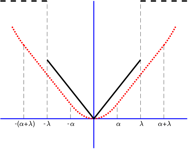
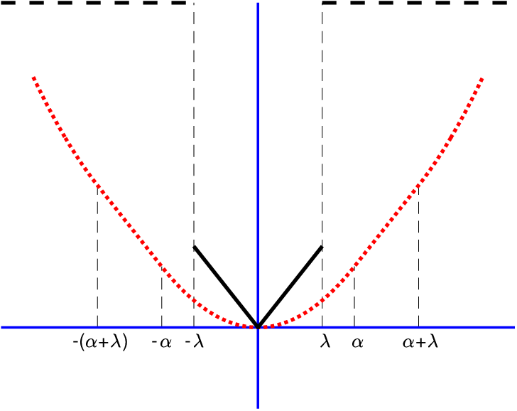
The last example is similar to the first one, but restricted to a cube centered at the origin. The function ff is given as follows: f⁡(x)=‖x‖1+ιC​(x),f(x)=\|x\|_{1}+\iota_{C}(x), where C=[−λ,λ]nC=[-\lambda,\lambda]^{n}. Generally speaking, this function promotes the sparsity on CC.

We notice that the function ff in the above four examples can be written as

f⁡(x)=∑i=1ng⁡(xi)f(x)=\sum_{i=1}^{n}g(x_{i})

for x∈ℝnx\in\mathbb{R}^{n} and some specific function gg. For example, gg is |⋅||\cdot|, max⁡{0,⋅}\max\{0,\cdot\}, 12|⋅|2+|⋅|\frac{1}{2}|\cdot|^{2}+|\cdot|, or |⋅|+ι[−λ,λ]|\cdot|+\iota_{[-\lambda,\lambda]}, in examples 1, 2, 3, or 4, an analogue of ff when ℝn\mathbb{R}^{n} reduces to ℝ\mathbb{R}. We further have that proxα​f(x)=proxα​g(x1)×proxα​g(x2)×⋯×proxα​g(xn)\prox_{\alpha f}(x)=\prox_{\alpha g}(x_{1})\times\prox_{\alpha g}(x_{2})\times\cdots\times\prox_{\alpha g}(x_{n}), envα​f⁡(x)=∑i=1nenvα​g⁡(xi)\env_{\alpha f}(x)=\sum_{i=1}^{n}\env_{\alpha g}(x_{i}), proxβ​fα(x)=proxβ​gα(x1)×proxβ​gα(x2)×⋯×proxβ​gα(xn)\prox_{\beta f_{\alpha}}(x)=\prox_{\beta g_{\alpha}}(x_{1})\times\prox_{\beta g_{\alpha}}(x_{2})\times\cdots\times\prox_{\beta g_{\alpha}}(x_{n}), and envβ​fα⁡(x)=∑i=1nenvβ​gα⁡(xi)\env_{\beta f_{\alpha}}(x)=\sum_{i=1}^{n}\env_{\beta g_{\alpha}}(x_{i}). Therefore, in the following discussion we will restrict ourself on n=1n=1.

6.1 Example 1: The absolute value function

The first example is the absolute value function f:ℝ→ℝ:x⟼|x|f:\mathbb{R}\rightarrow\mathbb{R}:x\longmapsto|x|, which is a special case of the piecewise quadratic function in ( Q ) with a1=a2=0a_{1}=a_{2}=0, b1=−1b_{1}=-1, and b2=1b_{2}=1. This function is nondifferentiable at the origin with argminx∈ℝ​f​(x)={0}\mathrm{argmin}_{x\in\mathbb{R}}f(x)=\{0\} and ∂f(0)=∂|⋅|(0)=[−1,1]\partial f(0)=\partial|\cdot|(0)=[-1,1].

Refer to caption Refer to caption
(a) (b)
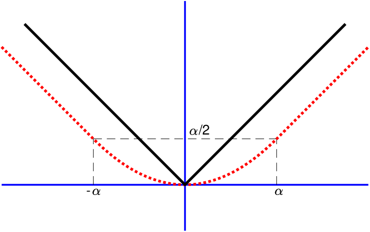
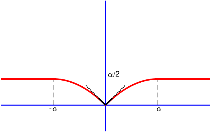
Figure 4: Example 1. (a) The graphs of ff (solid), envα​f\env_{\alpha f} (dotted), and (b) the graph of fα=f⁡(x)−envα​f​(x)f_{\alpha}=f(x)-\env_{\alpha f(x)}. Near the origin fαf_{\alpha} retains the structure of ff, which is emphasized in black (solid-dotted).

The proximity operator and the Moreau envelope of ff with parameter α>0\alpha>0 are

proxα|⋅|(x)=sgn(x)max{0,|x|−α}andenvα|⋅|(x)={12​α​x2,if |x|≤α;|x|−12​α,otherwise,\mathrm{prox}_{\alpha|\cdot|}(x)=\mathrm{sgn}(x)\max\{0,|x|-\alpha\}\quad\mbox{and}\quad\mathrm{env}_{\alpha|\cdot|}(x)=\left\{\begin{array}[]{ll}\frac{1}{2\alpha}x^{2},&\hbox{if $|x|\leq\alpha$;}\\ |x|-\frac{1}{2}\alpha,&\hbox{otherwise,}\end{array}\right.

respectively. It is well know that proxα|⋅|\mathrm{prox}_{\alpha|\cdot|} is called the soft thresholding in literature of wavelet [8] and envα|⋅|\mathrm{env}_{\alpha|\cdot|} is Huber’s function in robust statistics [14]. Figure 5 shows the typical shape of the proximity operator of ff.

Refer to caption
Figure 5: Example 1. The typical shape of proxα​f\prox_{\alpha f}.

As defined in ( F α ), for the absolute value function ff,

fα(x):=|x|−evnα|⋅|(x)={|x|−12​α​x2,if |x|≤α;12​α,otherwise.f_{\alpha}(x):=|x|-\mathrm{evn}_{\alpha|\cdot|}(x)=\left\{\begin{array}[]{ll}|x|-\frac{1}{2\alpha}x^{2},&\hbox{if $|x|\leq\alpha$;}\\ \frac{1}{2}\alpha,&\hbox{otherwise.}\end{array}\right.

This function fαf_{\alpha} (see Figure 4(b)) is identical to the minimax convex penalty (MCP) function given in [25], but motivated from statistic perspective.

The expression of proxβ​fα\mathrm{prox}_{\beta f_{\alpha}} depends on the relative values of α\alpha and β\beta. If β<α\beta<\alpha, Lemma 8 gives

proxβ​fα​(x)={0,if |x|≤β;αα−β​(|x|−β)​sgn​(x),if β<|x|≤α;x,if |x|≥α.\mathrm{prox}_{\beta f_{\alpha}}(x)=\left\{\begin{array}[]{ll}0,&\hbox{if $|x|\leq\beta$;}\\ \frac{\alpha}{\alpha-\beta}(|x|-\beta)\mathrm{sgn}(x),&\hbox{if $\beta<|x|\leq\alpha$;}\\ x,&\hbox{if $|x|\geq\alpha$.}\end{array}\right. (21)

This is the firm thresholding operator [12]. If β=α\beta=\alpha, Lemma 9 gives

proxβ​fα​(x)={0,if |x|<α;[0,α],if |x|=α;x,if |x|>α,\mathrm{prox}_{\beta f_{\alpha}}(x)=\left\{\begin{array}[]{ll}0,&\hbox{if $|x|<\alpha$;}\\ {[0,\alpha]},&\hbox{if $|x|=\alpha$;}\\ x,&\hbox{if $|x|>\alpha$,}\end{array}\right. (22)

Finally, if β>α\beta>\alpha, Lemma 10 gives

proxβ​fα​(x)={0,if |x|<α​β;{0,x},if |x|=α​β;x,if |x|>α​β;\mathrm{prox}_{\beta f_{\alpha}}(x)=\left\{\begin{array}[]{ll}0,&\hbox{if $|x|<\sqrt{\alpha\beta}$;}\\ \{0,x\},&\hbox{if $|x|=\sqrt{\alpha\beta}$;}\\ x,&\hbox{if $|x|>\sqrt{\alpha\beta}$;}\end{array}\right. (23)

The proximity operator proxβ​fα\mathrm{prox}_{\beta f_{\alpha}} for different values of α\alpha and β\beta is plotted in Figure 6.

Refer to caption Refer to caption Refer to caption
(a) (b) (c)
Figure 6: Typical shapes of the proximity operator of |⋅|α|\cdot|_{\alpha} for (a) β<α\beta<\alpha, (b) β=α\beta=\alpha, (c) β>α\beta>\alpha. The sparsity threshold and the thresholding behavior depend on the relationship between α\alpha and β\beta.

To end this example, we give several remarks on the proximity operators of proxα​f\mathrm{prox}_{\alpha f} and proxβ​fα\mathrm{prox}_{\beta f_{\alpha}} as follows:

  • •

    Note that ∂f⁡(0)=[−1,1]\partial f(0)=[-1,1]. The results given in (21) (for β<α\beta<\alpha) and (22) (for β=α\beta=\alpha) exactly match the first two statements of Theorem 2. For β>α\beta>\alpha, the proxβ​fα​(x)=0\mathrm{prox}_{\beta f_{\alpha}}(x)=0 for all x∈[−α​β,α​β]x\in[-\sqrt{\alpha\beta},\sqrt{\alpha\beta}] which includes the interval [−α,α]=α​∂f⁡(0)[-\alpha,\alpha]=\alpha\partial f(0) as indicated in the third statement of Theorem 2.

  • •

    The operator proxα​f\prox_{\alpha f} forces its variable to zero when the absolute value is less than a given threshold, and otherwise reduces the variable, in absolute value, by the amount of the threshold. Like proxα​f\prox_{\alpha f}, proxβ​fα\prox_{\beta f_{\alpha}} forces its variable to zero when the absolute value is less than a given threshold, but it fixes variables whose absolute value exceeds a certain threshold.

  • •

    For β≥α\beta\geq\alpha the proximity operator proxβ​fα\mathrm{prox}_{\beta f_{\alpha}} is almost identical to the hard threshold operator. Let |⋅|0|\cdot|_{0} be the ℓ0\ell_{0} “norm” on ℝ\mathbb{R}, that is, |x|0|x|_{0} equals 11 if xx is nonzero, 00 otherwise. The proximity operator of |⋅|0|\cdot|_{0} with parameter γ\gamma at xx is

    proxγ|⋅|0(x)={{0},if |x|<2​γ;{0,x},if |x|=2​γ;{x},if |x|>2​γ,\prox_{\gamma|\cdot|_{0}}(x)=\left\{\begin{array}[]{ll}\{0\},&\hbox{if $|x|<\sqrt{2\gamma}$;}\\ \{0,x\},&\hbox{if $|x|=\sqrt{2\gamma}$;}\\ \{x\},&\hbox{if $|x|>\sqrt{2\gamma}$,}\end{array}\right.

    which is called the hard thresholding operator with threshold 2​γ\sqrt{2\gamma}. We can see that proxγ|⋅|0=proxβ​fα\prox_{\gamma|\cdot|_{0}}=\mathrm{prox}_{\beta f_{\alpha}} as long as 2​γ=α​β2\gamma=\alpha\beta and β>α\beta>\alpha. It is interesting that although |⋅|0|\cdot|_{0} is discontinuous and fαf_{\alpha} is continuous, they have the same proximity operator. Moreover, by fixing α\alpha and varying the parameter β\beta, the proximity operator proxβ​fα\mathrm{prox}_{\beta f_{\alpha}} changes from the firm thresholding operator to the hard thresholding operator.

6.2 Example 2: ReLU function

The ReLU (Rectified Linear Unit) function on ℝ\mathbb{R} is

f⁡(x):=max⁡{0,x},f(x):=\max\{0,x\},

which is a special case of the piecewise quadratic function in ( Q ) with a1=b1=a2=0a_{1}=b_{1}=a_{2}=0 and b2=1b_{2}=1. The proximity operator and the Moreau envelope of ff with parameter α>0\alpha>0 are

proxα​f​(x)=min⁡{x,max⁡{0,x−α}}andenvα​f​(x)={0if x≤0;12​α​x2,if 0≤x≤α;x−12​α,if x≥α,\mathrm{prox}_{\alpha f}(x)=\min\{x,\max\{0,x-\alpha\}\}\quad\mbox{and}\quad\mathrm{env}_{\alpha f}(x)=\left\{\begin{array}[]{ll}0&\hbox{if $x\leq 0$;}\\ \frac{1}{2\alpha}x^{2},&\hbox{if $0\leq x\leq\alpha$;}\\ x-\frac{1}{2}\alpha,&\hbox{if $x\geq\alpha$,}\end{array}\right.

respectively. By ( F α ), fα​(x)=f⁡(x)−envα​f⁡(x)f_{\alpha}(x)=f(x)-\env_{\alpha f}(x) is

fα​(x)={0,if ​x<0x−12​α​x2,if ​0≤x≤αα2,if ​x>α\displaystyle f_{\alpha}(x)=\begin{cases}0,&\text{if }x<0\\ x-\frac{1}{2\alpha}x^{2},&\text{if }0\leq x\leq\alpha\\ \frac{\alpha}{2},&\text{if }x>\alpha\end{cases}

Figure 7(a) depicts the graphs of ff and envα​f\env_{\alpha f} while Figure 7(b) presents the function fαf_{\alpha}. The graph of proxα​f\prox_{\alpha f} is given in Figure 8.

Refer to caption Refer to caption
(a) (b)
Figure 7: Example 2. (a) The graphs of ff (solid), envα​f\env_{\alpha f} (dotted), and (b) their difference fα=f−envα​ff_{\alpha}=f-\env_{\alpha f}. The singularity of fαf_{\alpha} at zero is emphasized in black (solid-dotted).
Refer to caption
Figure 8: Example 2. The typical shape of proxα​f\prox_{\alpha f}. The parameter α\alpha is the sparsity threshold.

As in example 1, the expression of proxβ​fα\mathrm{prox}_{\beta f_{\alpha}} depends on the relative values of α\alpha and β\beta. If β<α\beta<\alpha,

proxβ​fα⁡(x)={x,if ​x≤0​ or ​x≥α;0,if ​0≤x≤β;α⁡(x−β)α−β;if ​β≤x≤α.\prox_{\beta f_{\alpha}}(x)=\begin{cases}x,&\text{if }x\leq 0\text{ or }x\geq\alpha;\\ 0,&\text{if }0\leq x\leq\beta;\\ \frac{\alpha(x-\beta)}{\alpha-\beta};&\text{if }\beta\leq x\leq\alpha.\end{cases} (24)

If β=α\beta=\alpha,

proxβ​fα⁡(x)={x,if ​x≤0​ or ​x>α;0,if ​0≤x<α;[0,α]if ​x=α.\prox_{\beta f_{\alpha}}(x)=\begin{cases}x,&\text{if }x\leq 0\text{ or }x>\alpha;\\ 0,&\text{if }0\leq x<\alpha;\\ [0,\alpha]&\text{if }x=\alpha.\end{cases} (25)

Finally, if β>α\beta>\alpha,

proxβ​fα⁡(x)={x,if ​x≤0​ or ​x>α​β;0,if ​0≤x<α​β;{0,α​β},if ​x=α​β.\prox_{\beta f_{\alpha}}(x)=\begin{cases}x,&\text{if }x\leq 0\text{ or }x>\sqrt{\alpha\beta};\\ 0,&\text{if }0\leq x<\sqrt{\alpha\beta};\\ \{0,\sqrt{\alpha\beta}\},&\text{if }x=\sqrt{\alpha\beta}.\end{cases} (26)
Refer to caption Refer to caption Refer to caption
(a) (b) (c)
Figure 9: Example 2. Typical shapes of the proximity operator of fαf_{\alpha} for (a) β<α\beta<\alpha; (b) β=α\beta=\alpha; and (c) β>α\beta>\alpha.

Note that ∂f⁡(0)=[0,1]\partial f(0)=[0,1]. The results given in (24) (for β<α\beta<\alpha) and (25) (for β=α\beta=\alpha) exactly match the first two statements of Theorem 2. For β>α\beta>\alpha, equation (26) shows that proxβ​fα​(x)=0\mathrm{prox}_{\beta f_{\alpha}}(x)=0 for all x∈[0,α​β]x\in[0,\sqrt{\alpha\beta}], which includes the interval [0,α]=α​∂f⁡(0)[0,\alpha]=\alpha\partial f(0) as indicated in the third statement of Theorem 2.

6.3 Example 3: Elastic Net

The elastic net is a regularized regression method in data analysis that linearly combines the ℓ1\ell_{1} and ℓ2\ell_{2} penalties of the LASSO and ridge methods. In this example, we consider a special case of the elastic net in ℝ\mathbb{R}:

f⁡(x)=12​x2+|x|.f(x)=\frac{1}{2}x^{2}+|x|.

This is an instance of the piecewise quadratic function given in ( Q ) with a1=a2=1a_{1}=a_{2}=1, b1=−1b_{1}=-1 and b2=1b_{2}=1. Clearly, ff is nondifferentiable at the origin with argminx∈ℝ​f​(x)={0}\mathrm{argmin}_{x\in\mathbb{R}}f(x)=\{0\}. Moreover, ∂f(0)=∂|⋅|(0)=[−1,1]\partial f(0)=\partial|\cdot|(0)=[-1,1].

The proximity operator and the Moreau envelope of ff with parameter α>0\alpha>0 are

proxα​f⁡(x)=max⁡{0,1α+1​(|x|−α)}​sgn⁡(x)andenvα​f⁡(x)={12​α​x2,if ​|x|≤α;1α+1​(12​x2+|x|−α2),if ​|x|≥α,\prox_{\alpha f}(x)=\max\left\{0,\frac{1}{\alpha+1}(|x|-\alpha)\right\}\sign(x)\quad\mbox{and}\quad\env_{\alpha f}(x)=\begin{cases}\frac{1}{2\alpha}x^{2},&\text{if }|x|\leq\alpha;\\ \frac{1}{\alpha+1}(\frac{1}{2}x^{2}+|x|-\frac{\alpha}{2}),&\text{if }|x|\geq\alpha,\\ \end{cases}

respectively.

The graphs of ff and envα​f\env_{\alpha f} are plotted in Figure 10 (a). The graph of proxα​f\prox_{\alpha f} is plotted in Figure 10 (b). As in the case of the absolute value function, proxα​f\prox_{\alpha f} sends all values between α\alpha and −α-\alpha to zero. Unlike the absolute value, it also contracts elements outside of this interval toward the origin.

Refer to caption Refer to caption
(a) (b)
Figure 10: Example 3. (a) The graphs of ff (solid) and envα​f\env_{\alpha f} (dotted); and (b) the graph of proxα​f\prox_{\alpha f}.

Now fαf_{\alpha}, the difference between ff and its Moreau envelope envα​f\env_{\alpha f}, is

fα​(x)={α−12​α​x2+|x|,if ​|x|≤α;α2​(α+1)​x2+αα+1​|x|+α2​(α+1),if ​|x|≥α.f_{\alpha}(x)=\begin{cases}\frac{\alpha-1}{2\alpha}x^{2}+|x|,&\text{if }|x|\leq\alpha;\\ \frac{\alpha}{2(\alpha+1)}x^{2}+\frac{\alpha}{\alpha+1}|x|+\frac{\alpha}{2(\alpha+1)},&\text{if }|x|\geq\alpha.\end{cases}

We remark that fαf_{\alpha} is convex when α≥1\alpha\geq 1 and nonconvex when α<1\alpha<1. The graph of fαf_{\alpha} for α≥1\alpha\geq 1 and α<1\alpha<1 are shown in Figure 11(a) and (b), respectively.

Refer to caption Refer to caption
(a) (b)
Figure 11: Example 3. The graph of fαf_{\alpha} when (a) α≥1\alpha\geq 1 and (b) α<1\alpha<1. The singularity of fαf_{\alpha} at zero is emphasized in black (solid-dotted).

According to the discussion given in subsection 5.2, we consider three cases: β⁡(α−1)+α>0\beta(\alpha-1)+\alpha>0, β⁡(α−1)+α=0\beta(\alpha-1)+\alpha=0, and β⁡(α−1)+α<0\beta(\alpha-1)+\alpha<0. These cases are equivalent to α⁡(β+1)>β\alpha(\beta+1)>\beta, α⁡(β+1)=β\alpha(\beta+1)=\beta, and α⁡(β+1)<β\alpha(\beta+1)<\beta respectively. Recall that these cases correspond to the convexity (or lack thereof) of fα​(u)+12​β​(u−x)2f_{\alpha}(u)+\frac{1}{2\beta}(u-x)^{2} for uu close to zero.

Case 1: α⁡(β+1)>β\alpha(\beta+1)>\beta. In this case, by Lemma 8 we have

proxβ​fα⁡(x)={0if ​|x|≤β;αα​β−β+α​(x−β​sgn⁡(x))if ​β≤|x|≤α⁡(β+1);α+1α​β+α+1​(x−α​βα+1​sgn⁡(x))if ​α​(β+1)≤|x|.\prox_{\beta f_{\alpha}}(x)=\begin{cases}0&\text{if }|x|\leq\beta;\\ \frac{\alpha}{\alpha\beta-\beta+\alpha}(x-\beta\sign(x))&\text{if }\beta\leq|x|\leq\alpha(\beta+1);\\ \frac{\alpha+1}{\alpha\beta+\alpha+1}(x-\frac{\alpha\beta}{\alpha+1}\sign(x))&\text{if }\alpha(\beta+1)\leq|x|.\end{cases} (27)

Case 2: α⁡(β+1)=β\alpha(\beta+1)=\beta. By Lemma 9 we have

proxβ​fα⁡(x)={0if ​|x|≤β;[0,α]​sgn⁡(x)if ​|x|=β;α+1α​β+α+1​(x−α​βα+1​sgn⁡(x))if ​β≤|x|.\prox_{\beta f_{\alpha}}(x)=\begin{cases}0&\text{if }|x|\leq\beta;\\ [0,\alpha]\sign(x)&\text{if }|x|=\beta;\\ \frac{\alpha+1}{\alpha\beta+\alpha+1}(x-\frac{\alpha\beta}{\alpha+1}\sign(x))&\text{if }\beta\leq|x|.\end{cases} (28)

Case 3: α⁡(β+1)<β\alpha(\beta+1)<\beta. Define

τ=α​βα+1+α​β​(α​β+α+1)α+1.\tau=\frac{\alpha\beta}{\alpha+1}+\frac{\sqrt{\alpha\beta(\alpha\beta+\alpha+1)}}{\alpha+1}. (29)

as in Lemma 10. Then we have

proxβ​fα⁡(x)={0if ​|x|≤τ;{0,ω}if ​|x|=τ;(α+1)​x−α​β​sgn⁡(x)α​β+α+1,if ​|x|>τ,\prox_{\beta f_{\alpha}}(x)=\begin{cases}0&\text{if }|x|\leq\tau;\\ \{0,\omega\}&\text{if }|x|=\tau;\\ \frac{(\alpha+1)x-\alpha\beta\sign(x)}{\alpha\beta+\alpha+1},&\text{if }|x|>\tau,\end{cases} (30)

where ω=(α+1)​τ−α​βα​β+α+1\omega=\frac{(\alpha+1)\tau-\alpha\beta}{\alpha\beta+\alpha+1}. The graphs of proxβ​fα\prox_{\beta f_{\alpha}} in the above three cases are plotted in Figure 12.

Refer to caption Refer to caption Refer to caption
(a) (b) (c)
Figure 12: Example 3. Typical shapes of proxβ​fα\prox_{\beta f_{\alpha}} when (a) α⁡(β+1)>β\alpha(\beta+1)>\beta, (b) α⁡(β+1)=β\alpha(\beta+1)=\beta, and (c) α⁡(β+1)<β\alpha(\beta+1)<\beta.

Below are some comments on this example.

  • •

    The function fαf_{\alpha} in the first two examples is nonconvex for any α>0\alpha>0, however, by Proposition 2 it is convex if α≥1\alpha\geq 1 due to our elastic net function ff being 11-strongly convex.

  • •

    The computation of the proximity operator proxβ​fα\prox_{\beta f_{\alpha}} is discussed under three different situations, namely, α⁡(β+1)>β\alpha(\beta+1)>\beta, α⁡(β+1)=β\alpha(\beta+1)=\beta, and α⁡(β+1)<β\alpha(\beta+1)<\beta. These situations are quite nature from Proposition 2. Since ff is 11-strongly convex, hence, the function fα+12​β(⋅−x)2f_{\alpha}+\frac{1}{2\beta}(\cdot-x)^{2} is (1+β−1−α−1)(1+\beta^{-1}-\alpha^{-1})-strongly convex if α⁡(β+1)>β\alpha(\beta+1)>\beta, convex if α⁡(β+1)=β\alpha(\beta+1)=\beta, and (α−1−1−β−1)(\alpha^{-1}-1-\beta^{-1})-semiconvex if α⁡(β+1)<β\alpha(\beta+1)<\beta.

  • •

    For the case of β≤α\beta\leq\alpha, we know that α⁡(1+β)>β\alpha(1+\beta)>\beta, so the proximity operator given (27) covers both statements 1 and 2 in Theorem 2.

  • •

    For the case of β>α\beta>\alpha, there are three possible related cases. If α<β<α⁡(β+1)\alpha<\beta<\alpha(\beta+1) (resp. α<β=α⁡(β+1)\alpha<\beta=\alpha(\beta+1)), the proximity operator given (27) (resp. (28)) shows that this operator vanishes all elements in β​∂f⁡(0)=[−β,β]⊃α​∂f⁡(0)\beta\partial f(0)=[-\beta,\beta]\supset\alpha\partial f(0), fulfilling the third statement of Theorem 2. If β>α⁡(β+1)\beta>\alpha(\beta+1), we know that α<1\alpha<1, β>α1−α\beta>\frac{\alpha}{1-\alpha}, and τ\tau defined in (29) satisfying

    τ=α​βα+1+α​β​(α​β+α+1)α+1>α21−α2+α1−α2>α.\tau=\frac{\alpha\beta}{\alpha+1}+\frac{\sqrt{\alpha\beta(\alpha\beta+\alpha+1)}}{\alpha+1}>\frac{\alpha^{2}}{1-\alpha^{2}}+\frac{\alpha}{1-\alpha^{2}}>\alpha.

    Hence, the proximity operator given (30) annihilates all elements in τ​∂f⁡(0)⊃α​∂f⁡(0)\tau\partial f(0)\supset\alpha\partial f(0), once again fulfilling the third statement of Theorem 2.

6.4 Example 4: Absolute value on an interval centered at the origin

Let λ\lambda be a positive parameter. The absolute function on the interval [−λ,λ][-\lambda,\lambda] centered at the origin is

f⁡(x):=|x|+ι[−λ,λ]​(x),f(x):=|x|+\iota_{[-\lambda,\lambda]}(x),

which is a special case given in ( ~ Q ) with a1=a2=0a_{1}=a_{2}=0, b1=−1b_{1}=-1, b2=1b_{2}=1, and C=[−λ,λ]C=[-\lambda,\lambda]. Its proximity operator and Moreau envelope with parameter α\alpha at point xx, respectively, are

proxα​f⁡(x)={0, if |x|≤α;sgn⁡(x)​(|x|−α), if α<|x|≤α+λ;λ​sgn⁡(x), if α+λ<|x|;\prox_{\alpha f}(x)=\begin{cases}0,&\text{ if $|x|\leq\alpha$;}\\ \sign(x)(|x|-\alpha),&\text{ if $\alpha<|x|\leq\alpha+\lambda$;}\\ \lambda\sign(x),&\text{ if $\alpha+\lambda<|x|$;}\end{cases}

and

envα​f⁡(x)={|x|−α2+12​α​(|x|−α)2, if |x|≤α;|x|−α2, if α<|x|≤α+λ;|x|−α2+12​α​(|x|−(λ+α))2, if α+λ<|x|.\env_{\alpha f}(x)=\begin{cases}|x|-\frac{\alpha}{2}+\frac{1}{2\alpha}(|x|-\alpha)^{2},&\text{ if $|x|\leq\alpha$;}\\ |x|-\frac{\alpha}{2},&\text{ if $\alpha<|x|\leq\alpha+\lambda$;}\\ |x|-\frac{\alpha}{2}+\frac{1}{2\alpha}(|x|-(\lambda+\alpha))^{2},&\text{ if $\alpha+\lambda<|x|$.}\end{cases}
Refer to caption Refer to caption Refer to caption
(a) (b) (c)
Figure 13: Example 4. The graphs of ff (solid, dashed) and envα​f\env_{\alpha f} (dotted) when (a) α<λ\alpha<\lambda and (b) α>λ\alpha>\lambda. The graph of proxα​f\prox_{\alpha f} is shown in (c). Between −(α+λ)-(\alpha+\lambda) and α+λ\alpha+\lambda, proxα​f\prox_{\alpha f} is the soft thresholding operator with sparsity parameter α\alpha; otherwise it projects onto this interval.

Figure 13 depicts the graphs of ff, envα​f\env_{\alpha f}, and proxα​f\prox_{\alpha f}. We observe that on the interval [−λ,λ][-\lambda,\lambda] (the domain of fαf_{\alpha}) the envelope envα​f\env_{\alpha f} is piecewise quadratic polynomial (Figure 13(a)) if α<λ\alpha<\lambda and is simply quadratic polynomial (Figure 13(b)) if α≥λ\alpha\geq\lambda. It turns out that the expression of proxβ​fα\prox_{\beta f_{\alpha}} for α<λ\alpha<\lambda is much more complicated than that for α≥λ\alpha\geq\lambda as we will see below.

As both ff and envα​f\env_{\alpha f} depend on α\alpha and λ\lambda, the explicit expression for fαf_{\alpha} will depend on the values of these parameters. To compute the proximity operator proxβ​fα\prox_{\beta f_{\alpha}}, we consider separately two main cases: α<λ\alpha<\lambda and α≥λ\alpha\geq\lambda.

Case 1: α<λ\alpha<\lambda. In this case, we get (see Figure 14)

fα​(x)=f⁡(x)−envα​f⁡(x)={α2−12​α​(|x|−α)2, if |x|≤α;α2, if a≤|x|≤λ;+∞, if λ<|x|.f_{\alpha}(x)=f(x)-\env_{\alpha f}(x)=\begin{cases}\frac{\alpha}{2}-\frac{1}{2\alpha}(|x|-\alpha)^{2},&\text{ if $|x|\leq\alpha$;}\\ \frac{\alpha}{2},&\text{ if $a\leq|x|\leq\lambda$;}\\ +\infty,&\text{ if $\lambda<|x|$.}\end{cases} (31)
Refer to caption
Figure 14: Example 4. The graph of fαf_{\alpha} when α<λ\alpha<\lambda with the singularity of fαf_{\alpha} at zero emphasized in black (solid-dotted). Further, we see that fαf_{\alpha} agrees with Example 1 on [−λ,λ][-\lambda,\lambda].

Depending on the values of α,β,\alpha,\beta, and λ\lambda, we consider four possible cases: β<α<λ\beta<\alpha<\lambda, β=α<λ\beta=\alpha<\lambda, α<β≤λ\alpha<\beta\leq\lambda, and λ<β\lambda<\beta.

Case 1.1: β<α<λ\beta<\alpha<\lambda. In this case, we have

proxβ​fα⁡(x)={max⁡{0,α⁡(|x|−β)α−β}​sgn⁡(x), if |x|≤α;min⁡{|x|,λ}​sgn⁡(x), if |x|>α.\prox_{\beta f_{\alpha}}(x)=\begin{cases}\max\{0,\frac{\alpha(|x|-\beta)}{\alpha-\beta}\}\sign(x),&\text{ if $|x|\leq\alpha$;}\\ \min\{|x|,\lambda\}\sign(x),&\text{ if $|x|>\alpha$.}\end{cases} (32)

Case 1.2: β=α<λ\beta=\alpha<\lambda. In this case, we have

proxβ​fα⁡(x)={0, if |x|<α;sgn⁡(x)​[0,α], if |x|=α;sgn⁡(x)​min​{|x|,λ}, if α<|x|,\prox_{\beta f_{\alpha}}(x)=\begin{cases}0,&\text{ if $|x|<\alpha$;}\\ \sign(x)[0,\alpha],&\text{ if $|x|=\alpha$;}\\ \sign(x)\min\{|x|,\lambda\},&\text{ if $\alpha<|x|$,}\end{cases} (33)

Case 1.3: α<β≤λ\alpha<\beta\leq\lambda. In this case, we have

proxβ​fα⁡(x)={0, if |x|<α​β;{0,sgn⁡(x)​α​β}, if |x|=α​β;min⁡{|x|,λ}​sgn⁡(x), if α​β<|x|,\prox_{\beta f_{\alpha}}(x)=\begin{cases}0,&\text{ if $|x|<\sqrt{\alpha\beta}$;}\\ \{0,\sign(x)\sqrt{\alpha\beta}\},&\text{ if $|x|=\sqrt{\alpha\beta}$;}\\ \min\{|x|,\lambda\}\sign(x),&\text{ if $\sqrt{\alpha\beta}<|x|$,}\end{cases} (34)

Case 1.4: α<λ<β\alpha<\lambda<\beta. We have

proxβ​fα⁡(x)={{0}, if |x|<α​β+λ22​λ;{0,λ​sgn⁡(x)}, if |x|=α​β+λ22​λ;{λ​sgn⁡(x)}, if α​β+λ22​λ<|x|,\prox_{\beta f_{\alpha}}(x)=\begin{cases}\{0\},&\text{ if $|x|<\frac{\alpha\beta+\lambda^{2}}{2\lambda}$;}\\ \{0,\lambda\sign(x)\},&\text{ if $|x|=\frac{\alpha\beta+\lambda^{2}}{2\lambda}$;}\\ \{\lambda\sign(x)\},&\text{ if $\frac{\alpha\beta+\lambda^{2}}{2\lambda}<|x|$,}\end{cases} (35)

We now move on to the second main case.

Case 2: λ≤α\lambda\leq\alpha. In this case, we get (see Figure 15)

fα​(x)={α2−12​α​(|x|−α)2, if |x|≤λ;+∞, otherwise.f_{\alpha}(x)=\begin{cases}\frac{\alpha}{2}-\frac{1}{2\alpha}(|x|-\alpha)^{2},&\text{ if $|x|\leq\lambda$;}\\ +\infty,&\text{ otherwise.}\end{cases}
Refer to caption
Figure 15: Example 4. The graph of fαf_{\alpha} when λ≤α\lambda\leq\alpha with the singularity of fαf_{\alpha} at zero emphasized in black (solid-dotted). As before, fαf_{\alpha} agrees with Example 1 on [−λ,λ][-\lambda,\lambda], but is cut off before it plateaus.

To compute proxβ​fα\prox_{\beta f_{\alpha}}, we consider three situations: β<α\beta<\alpha, β=α\beta=\alpha, and β>α\beta>\alpha.

Case 2.1: β<α\beta<\alpha. In this case, we have that

proxβ​fα⁡(x)={0, if |x|≤β;α⁡(|x|−β)α−β​sgn⁡(x), if β≤|x|≤β+α−βα​λ;λ​sgn⁡(x), if β+α−βα​λ≤|x|,\prox_{\beta f_{\alpha}}(x)=\begin{cases}0,&\text{ if $|x|\leq\beta$;}\\ \frac{\alpha(|x|-\beta)}{\alpha-\beta}\sign(x),&\text{ if $\beta\leq|x|\leq\beta+\frac{\alpha-\beta}{\alpha}\lambda$;}\\ \lambda\sign(x),&\text{ if $\beta+\frac{\alpha-\beta}{\alpha}\lambda\leq|x|,$}\end{cases} (36)

Case 2.2: β=α\beta=\alpha. In this case, we have

proxβ​fα⁡(x)={0, if |x|<α;sgn⁡(x)​[0,λ], if |x|=α;λ​sgn⁡(x), if α<|x|,\prox_{\beta f_{\alpha}}(x)=\begin{cases}0,&\text{ if $|x|<\alpha$;}\\ \sign(x)[0,\lambda],&\text{ if $|x|=\alpha$;}\\ \lambda\sign(x),&\text{ if $\alpha<|x|$,}\end{cases} (37)

Case 2.3: β>α\beta>\alpha. Similar to Case 1.4, we get

proxβ​fα⁡(x)={0, if |x|≤β−β−α2​α​λ;sgn⁡(x)​{0,λ}, if |x|=β−β−α2​α​λ;λ​sgn⁡(x), if β−β−α2​α​λ<|x|,\prox_{\beta f_{\alpha}}(x)=\begin{cases}0,&\text{ if $|x|\leq\beta-\frac{\beta-\alpha}{2\alpha}\lambda$;}\\ \sign(x)\{0,\lambda\},&\text{ if $|x|=\beta-\frac{\beta-\alpha}{2\alpha}\lambda$;}\\ \lambda\sign(x),&\text{ if $\beta-\frac{\beta-\alpha}{2\alpha}\lambda<|x|$,}\end{cases} (38)
Refer to caption Refer to caption Refer to caption
(a) (b) (c)
Figure 16: Example 4. Typical shapes of proxβ​fα\prox_{\beta f_{\alpha}} in (a) Case 1.1: β<α<λ\beta<\alpha<\lambda, (b) Case 2.2: β=α≥λ\beta=\alpha\geq\lambda, and (c) Case 1.3: α<β≤λ\alpha<\beta\leq\lambda. In each case, we see that the absolute threshold is λ\lambda, while the sparsity threshold and thresholding behavior depend on α\alpha and β\beta.

To end up this example, we comment on this example in a comparison with Theorem 2.

  • •

    Note that ∂f⁡(0)=[−1,1]\partial f(0)=[-1,1]. For β<α\beta<\alpha, both equations (32) and (36) show that the operator proxβ​fα\prox_{\beta f_{\alpha}} vanishes all elements in β​∂f⁡(0)=[−β,β]\beta\partial f(0)=[-\beta,\beta] as required by the first statement of Theorem 2.

  • •

    For β=α\beta=\alpha, both equations (33) and (37) show that the operator proxβ​fα\prox_{\beta f_{\alpha}} vanishes all elements in ri⁡(α​∂f⁡(0))=(−α,α)\mathrm{ri}(\alpha\partial f(0))=(-\alpha,\alpha) as described in the second statement of Theorem 2.

  • •

    For β>α\beta>\alpha, since α​β>α\sqrt{\alpha\beta}>\alpha, α​β+λ22​λ>α\frac{\alpha\beta+\lambda^{2}}{2\lambda}>\alpha when α<λ<β\alpha<\lambda<\beta, and β−β−α2​α​λ≥α\beta-\frac{\beta-\alpha}{2\alpha}\lambda\geq\alpha when α≥λ\alpha\geq\lambda, then equations (34), (34), and (38) shows that the operator proxβ​fα\prox_{\beta f_{\alpha}} vanishes all elements in ri⁡(α​∂f⁡(0))=(−α,α)\mathrm{ri}(\alpha\partial f(0))=(-\alpha,\alpha) as described in the third statement of Theorem 2.

To close this section, Table 1 lists the proximity operators proxβ​fα\prox_{\beta f_{\alpha}} of all examples.

Table 1: Proximity operators for all examples
Function β<α\beta<\alpha β=α\beta=\alpha β>α\beta>\alpha     
f⁡(x)=|x|f(x)=|x| (21) (22) (23)     
f⁡(x)=max⁡{0,x}f(x)=\max\{0,x\} (24) (25) (26)     
β<α⁡(β+1)\beta<\alpha(\beta+1) β=α⁡(β+1)\beta=\alpha(\beta+1) β>α⁡(β+1)\beta>\alpha(\beta+1)
f⁡(x)=12​x2+|x|f(x)=\frac{1}{2}x^{2}+|x| (27) (27) (27) (28) (30)
α<λ\alpha<\lambda α≥λ\alpha\geq\lambda α<λ\alpha<\lambda α≥λ\alpha\geq\lambda β≤λ\beta\leq\lambda β>λ\beta>\lambda α≥λ\alpha\geq\lambda
f⁡(x)=|x|+ι[−λ,λ]f(x)=|x|+\iota_{[-\lambda,\lambda]} (32) (36) (33) (37) (34) (35) (38)

‘

7 Conclusions

We presented a simple scheme to construct a family of semiconvex structured sparsity promoting functions from any convex sparsity promoting function. Theoretical guarantees of sparsity promotion were proved in Section 4, among other properties related to the structure of these functions. In Section 5, we expanded upon these results in the case of indicator and piecewise quadratic functions. We demonstrated that the classical MCP can be derived under this framework, while also providing several other examples motivated by a variety of applications.

Because of the structure of the proposed functions, we can use convex, nonconvex, and difference of convex algorithms in practice. We plan on testing these examples on problems such as signal denoising and variable selection. Furthermore, we hope to use the unique properties of these functions to develop new algorithms. Other future work will also expand upon the theoretical properties of these functions.

Disclaimer and Acknowledgment of Support

Any opinions, findings and conclusions or recommendations expressed in this material are those of the authors and do not necessarily reflect the views of AFRL (Air Force Research Laboratory).

Lixin Shen is partially supported by the US National Science Foundation under grant DMS-1522332.

References

  • [1] H. Attouch, J. Bolte, and B. Svaiter, Convergence of descent methods for semi-algebraic and tame problems: proximal algorithms, forward-backward splitting, and regularized gauss-seidel methods, Mathematical Programming, Ser. A, 137 (2013), pp. 91–129.
  • [2] H. L. Bauschke and P. L. Combettes, Convex Analysis and Monotone Operator Theory in Hilbert Spaces, AMS Books in Mathematics, Springer, New York, 2011.
  • [3] J. Bolte, A. Daniilidis, O. Ley, and L. Mazet, Characterizations of łojasiewicz inequalities: Subgradient flows, talweg, convexity, Transactions of the American Mathematical Society, 362 (2010), pp. 3319–3363.
  • [4] E. Candes and T. Tao, Near optimal signal recovery from random projections: Universal encoding strategies?, IEEE Transactions on Information Theory, 52 (2006), pp. 5406–5425.
  • [5] S. Chen, D. Donoho, and M. Saunders, Atomic decomposition by basis pursuit, SIAM Journal of Scientific Computing, 20 (1998), pp. 33–61.
  • [6] F. H. Clarke, Optimization and Nonsmooth Analysis, Wiley, New York, 1983.
  • [7] P. Combettes and V. Wajs, Signal recovery by proximal forward-backward splitting, Multiscale Modeling and Simulation: A SIAM Interdisciplinary Journal, 4 (2005), pp. 1168–1200.
  • [8] D. Donoho, Compressed sensing, IEEE Transactions on Information Theory, 52 (2006), pp. 1289–1306.
  • [9] D. Donoho and I. Johnstone, Ideal spatial adaptation by wavelet shrinkage, Biometrika, 81 (1994), pp. 425–455.
  • [10] J. Fan and R. Li, Variable selection via nonconcave penalized likelihood and its oracle properties, Journal of the American Statistical Association, 96 (2001), pp. 1348–1360.
  • [11] I. E. Frank and J. H. Friedman, A statistical view of some chemometrics regression tools (with discussion), Technometrics, 35 (1993), pp. 109–148.
  • [12] H.-Y. Gao and A. G. Bruce, WaveShrink with firm shrinkage, Statistica Sinica, 7 (1997), pp. 855–874.
  • [13] J.-B. Hiriart-Urruty and C. Lemarechal, Convex analysis and minimization algorithms I, vol. 305 of Grundlehren der Mathematischen Wissenschaften [Fundamental Principles of Mathematical Sciences], Springer-Verlag, Berlin, 1993.
  • [14] P. Huber, Robust Statistics, John Wiley & Sons Inc., Hoboken, New Jersey, second ed., 2009.
  • [15] S. Mallat, A Wavelet Tour of Signal Processing, Academic Press, New York, 2nd ed., 1999.
  • [16] C. A. Micchelli, L. Shen, and Y. Xu, Proximity algorithms for image models: Denoising, Inverse Problems, 27 (2011), p. 045009(30pp).
  • [17] J.-J. Moreau, Proximité et dualité dans un espace hilbertien, Bull. Soc. Math. France, 93 (1965), pp. 273–299.
  • [18] C. Planiden and X. Wang, Epi-convergence: The moreau envelope and generalized linear-quadratic functions, Journal of Optimization Theory and Applications, 177 (2018), pp. 21–63.
  • [19] G. Schwarz, Estimating the dimension of a model, The Annals of Statistics, 6 (1978), pp. 461–464.
  • [20] I. Selesnick, Total variation denoising via the moreau envelope, IEEE Signal Processing Letters, 24 (2017), pp. 216–220.
  • [21] E. Soubies, L. Blanc-Feraud, and G. Aubert, A unified view of exact continuous penalties for ℓ2\ell_{2}-ℓ0\ell_{0} minimization, SIAM Journal on Optimization, 27 (2017), pp. 2034–2060.
  • [22] B. W. Suter, Multirate and wavelet signal processing, Academic Press, 1997.
  • [23] P. Tao and H. Le Thi, Convex analysis approach to dc programming: Theory, algorithms and applications, Acta Mathematica Vietnamica, 22 (1997), pp. 289–355.
  • [24] R. Tibshirani, Regression shrinkage and selection via the LASSO, Journal of the Royal Statistical Society, Series B, 58 (1996), pp. 267–288.
  • [25] C.-H. Zhang, Nearly unbiased variable selection under minimax concave penalty, Annals of Statistics, 38 (2010), pp. 894–942.
  • [26] H. Zou and T. Hastie, Regularization and variable selection via the elastic net, Journal of the Royal Statistical Society, Series B, 67 (2005), pp. 301–320.