跳到论文正文
W Papers独立论文阅读器 arXiv:1809.06525 论文正文 计算阅读时间 · 0%
引用这篇论文根据当前论文元数据生成,正式投稿前建议核对。


License: arXiv.org perpetual non-exclusive license
arXiv:1809.06525v4 [math.FA] 12 Feb 2019

Convergence analysis of a variable metric forward-backward splitting algorithm with applications

Fuying Cui Affiliation:  Department of Mathematics, Nanchang University, Nanchang 330031, P.R. China    Yuchao Tang Affiliation:  Department of Mathematics, Nanchang University, Nanchang 330031, P.R. China    Chuanxi Zhu Affiliation:  Department of Mathematics, Nanchang University, Nanchang 330031, P.R. China

Abstract. The forward-backward splitting algorithm is a popular operator-splitting method for solving monotone inclusion of the sum of a maximal monotone operator and a cocoercive operator. In this paper, we present a new convergence analysis of a variable metric forward-backward splitting algorithm with extended relaxation parameters in real Hilbert spaces. We prove that this algorithm is weakly convergent when certain weak conditions are imposed upon the relaxation parameters. Consequently, we recover the forward-backward splitting algorithm with variable step sizes. As an application, we obtain a variable metric forward-backward splitting algorithm for solving the minimization problem of the sum of two convex functions, where one of them is differentiable with a Lipschitz continuous gradient. Furthermore, we discuss the applications of this algorithm to the fundamental of the variational inequalities problem, constrained convex minimization problem, and split feasibility problem. Numerical experimental results on LASSO problem in statistical learning demonstrate the effectiveness of the proposed iterative algorithm.

Key words: Forward-backward splitting algorithm; Monotone inclusion; Variable metric; Split feasibility problem.

AMS Subject Classification: 90C25; 47H05.

1 Introduction

Let HH be a real Hilbert space. The forward-backward splitting algorithm is a classical operator-splitting algorithm, which solves the monotone inclusion problem,

find​x∈H,such that​ 0∈A​x+B​x,\textrm{find}\,x\in H,\quad\textrm{such that}\,0\in Ax+Bx, (1.1)

where A:H→2HA:H\rightarrow 2^{H} is a maximal monotone operator and B:H→HB:H\rightarrow H is a β\beta-cocoercive operator, for some β>0\beta>0. The forward-backward splitting algorithm, which dates back to the original work of Lions and Mercier [1], has been studied and reported extensively in the literature, for example [2, 3, 4, 5, 6]. The emergence of compressive sensing theory and large-scale optimization problems associated with signal and image processing has resulted in the forward-backward splitting algorithm receiving much attention in recent years. A forward-backward splitting algorithm with relaxation and errors in Hilbert spaces was proposed by Combettes [4]. More precisely, let x0∈Hx_{0}\in H, set

xk+1=xk+λk​(Jγk​A​(xk−γk​(B​xk+bk))+ak−xk),k≥0,x_{k+1}=x_{k}+\lambda_{k}(J_{\gamma_{k}A}(x_{k}-\gamma_{k}(Bx_{k}+b_{k}))+a_{k}-x_{k}),\quad k\geq 0, (1.2)

where {γk}⊂(0,2​β)\{\gamma_{k}\}\subset(0,2\beta), {λk}⊂(0,1]\{\lambda_{k}\}\subset(0,1], {ak}\{a_{k}\} and {bk}\{b_{k}\} are absolutely summable sequences in HH. In addition, Jγk​A:=(I+γk​A)−1J_{\gamma_{k}A}:=(I+\gamma_{k}A)^{-1} denotes the resolvent of operator AA with index γk>0\gamma_{k}>0. Combettes [4] proved the convergence of the iterative scheme (1.2) when certain conditions are imposed upon the parameters. Jiao and Wang [7] generalized the iterative scheme (1.2) by extending the work of Combettes [4]. They proved the convergence of (1.2) by requiring the parameters {λk}\{\lambda_{k}\} to comply with the requirement {λk}⊂(0,4​β2​β+γk)\{\lambda_{k}\}\subset\left(0,\frac{4\beta}{2\beta+\gamma_{k}}\right) when bk=0b_{k}=0. It is easy to see that 4​β2​β+γk\frac{4\beta}{2\beta+\gamma_{k}} is strictly larger than one when {γk}⊂(0,2​β)\{\gamma_{k}\}\subset(0,2\beta). Further, Combettes and Yamada [8] improved the range of the relaxation parameters {λk}\{\lambda_{k}\} in (1.2) to (0,4​β−γk2​β)(0,\frac{4\beta-\gamma_{k}}{2\beta}). After a simple calculation, we know that 4​β−γk2​β>4​β2​β+γk\frac{4\beta-\gamma_{k}}{2\beta}>\frac{4\beta}{2\beta+\gamma_{k}}. Therefore, the range of {λk}\{\lambda_{k}\} in the work of Combettes and Yamada [8] is larger than that of Jiao and Wang [7].

In the case when γk=γ\gamma_{k}=\gamma and ak=bk=0a_{k}=b_{k}=0, the iterative scheme (1.2) is reduced to the forward-backward splitting algorithm with a constant step size [9],

xk+1=xk+λk​(Jγ​A​(xk−γ​B​xk)−xk),k≥0,x_{k+1}=x_{k}+\lambda_{k}(J_{\gamma A}(x_{k}-\gamma Bx_{k})-x_{k}),\quad k\geq 0, (1.3)

where γ∈(0,2​β)\gamma\in(0,2\beta) and {λk}⊂(0,4​β−γ2​β)\{\lambda_{k}\}\subset(0,\frac{4\beta-\gamma}{2\beta}). Bauschke and Combettes [9] obtained the convergence of the iterative algorithm (1.3) by adopting the Krasnosekiĭ-Mann iteration for computing the fixed points of nonexpansive operators. The forward-backward splitting algorithm with constant step size (1.3) is usually considered to be stationary, whereas the forward-backward splitting algorithm with variable step sizes (1.2) is referred to as non-stationary.

It is worth mentioning that by letting λk=1\lambda_{k}=1, then (1.3)(\ref{relax-forward-backward-constant}) reduces to the classical forward-backward splitting algorithm. More precisely, the iterative sequence {xk}\{x_{k}\} is defined by

xk+1=Jγ​A​(xk−γ​B​xk),k≥0.x_{k+1}=J_{\gamma A}(x_{k}-\gamma Bx_{k}),\quad k\geq 0. (1.4)

In the context of convex optimization, the forward-backward splitting algorithm is equivalent to the so-called proximal gradient algorithm (PGA) applied to solve the following convex minimization problem,

minx∈H⁡f⁡(x)+g⁡(x),\min_{x\in H}f(x)+g(x), (1.5)

where f:H→Rf:H\rightarrow R is convex, differentiable with an LL-Lipschitz continuous gradient for some L>0L>0 and g:H→(−∞,+∞]g:H\rightarrow(-\infty,+\infty] is a proper, lower semicontinuous, convex function. The convex optimization problem (1.5) has found widespread application in signal and image processing, for example [10, 11, 12]. As a consequence of [4], Combettes and Wajs [13] employed the forward-backward splitting algorithm (1.2) to solve the minimization problem (1.5). The obtained iterative algorithm is defined as

xk+1=xk+λk​(p​r​o​xγk​g​(xk−γk​(∇f​(xk)+bk))+ak−xk),k≥0,x_{k+1}=x_{k}+\lambda_{k}(prox_{\gamma_{k}g}(x_{k}-\gamma_{k}(\nabla f(x_{k})+b_{k}))+a_{k}-x_{k}),\quad k\geq 0, (1.6)

where {γk}⊂(0,2/L)\{\gamma_{k}\}\subset(0,2/L), {λk}⊂(0,1]\{\lambda_{k}\}\subset(0,1], and {ak}\{a_{k}\}, {bk}\{b_{k}\} are absolutely summable sequences in HH. p​r​o​xγ​gprox_{\gamma g} denotes the proximity operator of gg with index γ>0\gamma>0. In addition, Combettes and Wajs [13] presented applications of this algorithm to many concrete convex optimization problems. This iterative algorithm (1.6) was subsequently improved by Combettes and Yamada [8] who extended the range of the relaxation parameters {λk}\{\lambda_{k}\}.

Inspired by solving large-scale convex optimization problems arising in image processing, machine learning, and economic management, many efficient primal-dual splitting algorithms have been proposed for structured monotone inclusions involving maximal monotone operators and single-valued Lipschitz or cocoercive monotone operators, for example [14, 15]. Although these monotone inclusions are more complicated than the monotone inclusion problem (1.1), they can be transformed into the form of this problem in a suitable product space. Therefore, it is natural to consider using the forward-backward splitting algorithm (e.g., (1.2) or (1.3)) to solve the equivalent monotone inclusion problem. Because the backward steps cannot be decomposed, direct use of the forward-backward splitting algorithm often fails to obtain a completely splitting algorithm. Many researchers attempted to overcome this difficulty by investigating variable metric operator splitting algorithms. The use of a suitable variable metric enables the implicit step of backward splitting to be easily decomposed. For example, the primal-dual hybrid gradient algorithm [16] (also known as the primal-dual of the Chambolle-Pock algorithm [17]) is equivalent to the variable metric proximal point algorithm [18, 19]. We refer the readers to a subsequent paper [20] for more details. Vũ [21] proposed a variable metric extension of the forward-backward-forward splitting algorithm [3] for solving monotone inclusion of the sum of a maximal monotone operator and a monotone Lipschitzian operator in Hilbert spaces. Liang [22] proposed a variable metric multi-step inertial operator-splitting algorithm for solving the monotone inclusion problem (1.1). Bonettini et al. [23] developed a scaled inertial forward-backward splitting algorithm for solving (1.1) in the context of convex minimization. Neither of the respective algorithms in the work by Liang [22] and Bonettini et al. [23] was compatible with the relaxation strategy. The variable metric forward-backward splitting algorithm was originally studied in finite-dimensional Hilbert spaces [2, 24]; however, the methods in these studies either had to be strongly monotone to study the convergence rate or they did not make use of the cocoercive property of BB in (1.1). For infinite-dimensional Hilbert spaces, Combettes and Vũ [25] proposed a variable metric forward-backward splitting algorithm to solve (1.1) and analyzed its weak and strong convergence. This algorithm is defined as follows. Let x0∈Hx_{0}\in H, and set

{yk=xk−γk​Uk​(B​xk+bk),xk+1=xk+λk​(Jγk​Uk​A​(yk)+ak−xk).\left\{\begin{aligned} y_{k}&=x_{k}-\gamma_{k}U_{k}(Bx_{k}+b_{k}),\\ x_{k+1}&=x_{k}+\lambda_{k}(J_{\gamma_{k}U_{k}A}(y_{k})+a_{k}-x_{k}).\end{aligned}\right. (1.7)

where {Uk}⊂𝒫α​(H)\{U_{k}\}\subset\mathcal{P}_{\alpha}(H), {λk}⊂(0,1]\{\lambda_{k}\}\subset(0,1], {γk}⊂(0,2​β)\{\gamma_{k}\}\subset(0,2\beta), {ak}\{a_{k}\} and {bk}\{b_{k}\} are absolutely summable sequences in HH. This algorithm (1.7) includes a variable metric, variable step sizes, relaxation parameter, and errors. It includes nearly all of the forward-backward type of splitting algorithms mentioned above. For example, by letting Uk=IU_{k}=I in (1.7), it is reduced to (1.2). The relaxation parameters {λk}\{\lambda_{k}\} in (1.2) are observed to be strictly larger than that based on the work of Combettes and Yamada [8]. While preparing this manuscript, we discovered that in Chapter 5 of the dissertation [26], Simões generalized the variable metric forward-backward splitting algorithm by replacing the relaxation parameters {λk}\{\lambda_{k}\} in (1.7) with self-adjoint, strong positive linear operators. However, this approach still requires the maximum eigenvalue of the operators to be smaller than one.

The purpose of this paper is to introduce a new convergence analysis for the variable metric forward-backward splitting algorithm (1.7) with an extended range of relaxation parameters. We prove the weak convergence of the variable metric forward-backward splitting algorithm by setting the relaxation parameter {λk}\{\lambda_{k}\} larger than one in real Hilbert spaces. To achieve this goal, we make full use of the averaged and firmly nonexpansive property of operators Jγk​Uk​A​(I−γk​Uk​B)J_{\gamma_{k}U_{k}A}(I-\gamma_{k}U_{k}B) and Jγk​Uk​AJ_{\gamma_{k}U_{k}A}, where λk>0\lambda_{k}>0 and Uk∈𝒫α​(H)U_{k}\in\mathcal{P}_{\alpha}(H). In contrast, existing solutions mainly rely on Jγk​Uk​AJ_{\gamma_{k}U_{k}A} being firmly nonexpansive. Consequently, we obtain the convergence of the forward-backward splitting algorithm with variable step sizes. Moreover, we impose a slightly weak condition on the relaxation parameters to ensure the convergence of this algorithm. The results we obtained complement and extend those of Combettes and Yamada [8]. As an application, we obtain the variable metric forward-backward splitting algorithm for solving the minimization problem (1.5). We also present the application of this algorithm to the variational inequalities problem, constrained convex minimization problem, and split feasibility problem. To the best of our knowledge, the iterative algorithms we obtained are the most general ones for solving these problems. Finally, we conduct numerical experiments on LASSO problem to validate the effectiveness of the proposed iterative algorithm.

The remainder of this paper is organized as follows. Section 22 reviews selected notations and lemmas on monotone operator theory and presents some technical lemmas. In Section 33, we prove the main convergence results of the variable metric forward-backward splitting algorithm with relaxation in real Hilbert spaces. Consequently, we obtain several corollaries of some special cases. Section 44 presents our use of the proposed iterative algorithm to solve three typical optimization problems include the variational inequalities problem, constrained convex minimization problem, and split feasibility problem. In Section 55, we present preliminary numerical results on LASSO problem to illustrate the performance of the proposed iterative algorithm. Finally, we provide our conclusions.

2 Preliminaries

In this section, we recall selected concepts and lemmas that are commonly used in the context of convex analysis and monotone operator theory. Most of them can be found in [27, 9]. Throughout this paper, let HH be a real Hilbert space. The inner product and the associated norm of Hilbert space HH are denoted by ⟨⋅,⋅⟩\langle\cdot,\cdot\rangle and ∥⋅∥\|\cdot\|, respectively. II denotes the identity operator and the symbols ⇀\rightharpoonup and →\rightarrow denote weak and strong convergence.

We first recall selected basic notations and definitions. Let A:H→2HA:H\rightarrow 2^{H} be a set-valued operator. We denote its domain, range, graph, and zeros by dom A={x∈H|A​x≠∅}A=\{x\in H|Ax\neq\emptyset\}, ran A={u∈H|(∃x∈H)​u∈A​x}A=\{u\in H|(\exists x\in H)u\in Ax\}, gra A={(x,u)∈H×H|u∈A​x}A=\{(x,u)\in H\times H|u\in Ax\}, and zer A={x∈H|0∈A​x}A=\{x\in H|0\in Ax\}, respectively.

Definition 2.1.

Let A:H→2HA:H\rightarrow 2^{H} be a set-valued operator. AA is said to be monotone, if

⟨x−y,u−v⟩≥0,∀(x,u),(y,v)∈gra ​A.\langle x-y,u-v\rangle\geq 0,\quad\forall(x,u),(y,v)\in\textrm{gra }A.

Moreover, AA is said to be maximal monotone, if its graph is not strictly contained in the graph of any other monotone operator on HH.

A well-known example of a maximal monotone operator is the subgradient mapping of a proper, lower semicontinuous convex function f:H→(−∞,+∞]f:H\rightarrow(-\infty,+\infty] defined by

∂f:H→2H:x↦{u∈H|f(y)≥f(x)+⟨u,y−x⟩,∀y∈H}.\partial f:H\rightarrow 2^{H}:x\mapsto\{u\in H|f(y)\geq f(x)+\langle u,y-x\rangle,\forall y\in H\}.
Definition 2.2.

Let A:H→2HA:H\rightarrow 2^{H} be a maximal monotone operator. The resolvent operator of AA with index λ>0\lambda>0 is defined as

Jλ​A=(I+λ​A)−1.J_{\lambda A}=(I+\lambda A)^{-1}.

According to the Minty theorem, the resolvent operator Jλ​AJ_{\lambda A} is defined everywhere on Hilbert space HH, and Jλ​AJ_{\lambda A} is firmly nonexpansive.

Let us recall the definition of the proximity operator, which was first introduced by Moreau [28]. Let f∈Γ0​(H)f\in\Gamma_{0}(H), where Γ0​(H)\Gamma_{0}(H) denotes the set of all proper lower semicontinuous convex functions f:H→(−∞,+∞]f:H\rightarrow(-\infty,+\infty]. The proximity operator of ff with index λ>0\lambda>0 is defined by

p​r​o​xλ​f:H→H:x↦arg⁡miny∈H​12​‖y−x‖2+λ​f​(y).prox_{\lambda f}:H\rightarrow H:x\mapsto\arg\min_{y\in H}\frac{1}{2}\|y-x\|^{2}+\lambda f(y).

In fact, the resolvent operator of the subdifferential operator of any f∈Γ0​(H)f\in\Gamma_{0}(H) with index λ>0\lambda>0 is the proximal operator of ff with index λ>0\lambda>0, that is

p​r​o​xλ​f=(I+λ​∂f)−1.prox_{\lambda f}=(I+\lambda\partial f)^{-1}.

Therefore, the proximity operators have the same property as the resolvent operators.

Definition 2.3.

Let B:H→HB:H\rightarrow H be a single-valued operator. Let β>0\beta>0, then BB is said to be β\beta-cocoercive, if

⟨x−y,B​x−B​y⟩≥β​‖B​x−B​y‖2,∀x,y∈H.\langle x-y,Bx-By\rangle\geq\beta\|Bx-By\|^{2},\quad\forall x,y\in H.

The β\beta-cocoercive operator is also known as a β\beta-inverse strongly monotone operator (β\beta-ism), for example [29]. It is easy to see from the above definition that a β\beta-cocoercive operator is 1β\frac{1}{\beta}-Lipschitz continuous, i.e., ‖B​x−B​y‖≤1β​‖x−y‖\|Bx-By\|\leq\frac{1}{\beta}\|x-y\|.

Next, we recall the definitions of nonexpansive and related mappings. These mappings often appear in the convergence analysis of optimization algorithms.

Definition 2.4.

Let CC be a nonempty subset of HH. Let T:C→HT:C\rightarrow H, then

(i) TT is considered to be nonexpansive, if

‖T​x−T​y‖≤‖x−y‖,∀x,y∈C.\|Tx-Ty\|\leq\|x-y\|,\quad\forall x,y\in C.

(ii) TT is considered to be firmly nonexpansive, if

‖T​x−T​y‖2≤‖x−y‖2−‖(I−T)​x−(I−T)​y‖2,∀x,y∈C.\|Tx-Ty\|^{2}\leq\|x-y\|^{2}-\|(I-T)x-(I-T)y\|^{2},\quad\forall x,y\in C.

(iii) TT is referred to as α\alpha-averaged, α∈(0,1)\alpha\in(0,1), if there exists a nonexpansive mapping SS such that T=(1−α)​I+α​ST=(1-\alpha)I+\alpha S.

It follows immediately that a firmly nonexpansive mapping is a nonexpansive mapping and an α\alpha-averaged mapping is also nonexpansive.

We denote by F​i​x​(T)Fix(T) the set of fixed pints of a mapping TT, that is F​i​x​(T)={x∈H|x=T​x}Fix(T)=\{x\in H|x=Tx\}.

Lemma 2.1.

(Demiclosedness Principle) Let CC be a nonempty subset of HH. Let T:C→HT:C\rightarrow H be a nonexpansive mapping with F​i​x​(T)≠∅Fix(T)\neq\emptyset. If {xk}\{x_{k}\} is a sequence in CC that converges weakly to xx and if {(I−T)​xk}\{(I-T)x_{k}\} converges strongly to yy, then (I−T)​x=y(I-T)x=y; in particular, if y=0y=0, then x∈F​i​x​(T)x\in Fix(T).

The following proposition provides some equivalent definitions of the firmly nonexpansive mappings. This proposition can be found in Proposition 4.2 of [27].

Proposition 2.1.

Let CC be a nonempty subset of HH. Let T:C→HT:C\rightarrow H, then the following are equivalent

(i) TT is firmly nonexpansive;

(ii) I−TI-T is firmly nonexpansive;

(iii) 2​T−I2T-I is nonexpansive;

(iv) ⟨x−y,T​x−T​y⟩≥‖T​x−T​y‖2,∀x,y∈C\langle x-y,Tx-Ty\rangle\geq\|Tx-Ty\|^{2},\quad\forall x,y\in C;

From Proposition 2.1 (iii) and (iv), we know that if TT is firmly nonexpansive, then TT is 12\frac{1}{2}-averaged, and a 11-cocoercive operator is firmly nonexpansive.

The following proposition is taken from Proposition 4.25 of [27].

Proposition 2.2.

Let CC be a nonempty subset of HH. Let T:C→HT:C\rightarrow H, then TT is α\alpha-averaged if and only if

‖T​x−T​y‖2≤‖x−y‖2−1−αα​‖(I−T)​x−(I−T)​y‖,∀x,y∈C.\|Tx-Ty\|^{2}\leq\|x-y\|^{2}-\frac{1-\alpha}{\alpha}\|(I-T)x-(I-T)y\|,\quad\forall x,y\in C.

.

The following lemma provides a relation between an operator TT with its complement I−TI-T.

Lemma 2.2.

Let CC be a nonempty subset of HH. Let T:C→HT:C\rightarrow H, then

(i) TT is nonexpansive if and only if the complement I−TI-T is 12\frac{1}{2}-cocoercive;

(ii) TT is α\alpha-averaged if and only if the complement I−TI-T is 12​α\frac{1}{2\alpha}-cocoercive.

We refer interested readers to [27] for further properties of nonexpansive, firmly nonexpansive, and α\alpha-averaged nonlinear mappings.

We recall the results of the composition of two averaged operators. The following lemma first appeared in [30] after which it was extended to a finite family of composition-averaged operators [8].

Lemma 2.3.

Let CC be a nonempty subset of HH. Let T1:C→HT_{1}:C\rightarrow H is α1\alpha_{1}-averaged and T2:C→HT_{2}:C\rightarrow H is α2\alpha_{2}-averaged. Then

T:=T1​T2​ is ​α1+α2−2​α1​α21−α1​α2−averaged.T:=T_{1}T_{2}\textrm{ is }\frac{\alpha_{1}+\alpha_{2}-2\alpha_{1}\alpha_{2}}{1-\alpha_{1}\alpha_{2}}-\textrm{averaged}.
Remark 2.1.

(i) It is worth mentioning that two other results of the combination of averaged operators were reported. From Proposition 4.32 of [27], T:=T1​T2T:=T_{1}T_{2} is α¯=21+1max⁡(α1,α2)\overline{\alpha}=\frac{2}{1+\frac{1}{\max(\alpha_{1},\alpha_{2})}}-averaged. From Byrne [29], T:=T1​T2T:=T_{1}T_{2} is α^=α1+α2−α1​α2\widehat{\alpha}=\alpha_{1}+\alpha_{2}-\alpha_{1}\alpha_{2}-averaged. It is not difficult to verify that α1+α2−2​α1​α21−α1​α2\frac{\alpha_{1}+\alpha_{2}-2\alpha_{1}\alpha_{2}}{1-\alpha_{1}\alpha_{2}} is smaller than the other two constants α¯\overline{\alpha} and α^\widehat{\alpha}.

(ii) The constant α^\widehat{\alpha} is used in [7] to show the upper bound of the relaxation parameter λk\lambda_{k} such that λk<1α^\lambda_{k}<\frac{1}{\widehat{\alpha}}.

We employ the following previously used notation [25]. Let ℬ⁡(H,G)\mathcal{B}(H,G) be the spaces of bounded linear operators from Hilbert space HH to Hilbert space GG. The norm of L∈ℬ⁡(H,G)L\in\mathcal{B}(H,G) is defined as ‖L‖=supx∈H‖L​x‖‖x‖\|L\|=\sup_{x\in H}\frac{\|Lx\|}{\|x\|}. We set ℬ⁡(H)=ℬ⁡(H,H)\mathcal{B}(H)=\mathcal{B}(H,H) and 𝕊⁡(H)={L∈ℬ⁡(H)|L=L∗}\mathbb{S}(H)=\{L\in\mathcal{B}(H)|L=L^{*}\}, where L∗L^{*} denotes the adjoint of LL. The Loewner partial ordering on S⁡(H)S(H) is defined by, for any U,V∈S⁡(H)U,V\in S(H),

U⪰V⇔⟨U​x,x⟩≥⟨V​x,x⟩,∀x∈H.U\succeq V\Leftrightarrow\langle Ux,x\rangle\geq\langle Vx,x\rangle,\forall x\in H.

Let α∈[0,+∞)\alpha\in[0,+\infty), set

𝒫α​(H)={U∈S⁡(H)|U⪰α​I}.\mathcal{P}_{\alpha}(H)=\{U\in S(H)|U\succeq\alpha I\}.

We denote U\sqrt{U} as the square root of U∈𝒫α​(H)U\in\mathcal{P}_{\alpha}(H). Moreover, for every U∈𝒫α​(H)U\in\mathcal{P}_{\alpha}(H), we define a semi-scalar product and a semi-norm (a scalar product and a norm , if α>0\alpha>0 by

(∀x∈H)​(∀y∈H)⟨x,y⟩U=⟨U​x,y⟩a​n​d‖x‖U=⟨U​x,x⟩.(\forall x\in H)(\forall y\in H)\quad\langle x,y\rangle_{U}=\langle Ux,y\rangle\quad and\quad\left\|x\right\|_{U}=\sqrt{\langle Ux,x\rangle}.

We borrow the following results on monotone operators in a variable metric setting from Combettes’s work [25].

Lemma 2.4.

Let A:H→2HA:H\rightarrow 2^{H} be maximal monotone, let α∈(0,+∞)\alpha\in(0,+\infty), let U∈𝒫α​(H)U\in\mathcal{P}_{\alpha}(H) and let HU−1H_{U^{-1}} be the real Hilbert space with the scalar product ⟨x,y⟩U−1=⟨U−1​x,y⟩,∀x,y∈H\langle x,y\rangle_{U^{-1}}=\langle U^{-1}x,y\rangle,\forall x,y\in H. Then the following hold:

(i) U​A:H→2HUA:H\rightarrow 2^{H} is maximal monotone;

(ii) JU​A:H→2HJ_{UA}:H\rightarrow 2^{H} is 11-cocoercive, i.e., firmly nonexpansive. More precisely,

‖JU​A​x−JU​A​y‖U−12≤‖x−y‖U−12−‖(I−JU​A)​x−(I−JU​A)​y‖U−12,∀x,y∈H.\|J_{UA}x-J_{UA}y\|^{2}_{U^{-1}}\leq\|x-y\|^{2}_{U^{-1}}-\|(I-J_{UA})x-(I-J_{UA})y\|^{2}_{U^{-1}},\quad\forall x,y\in H. (2.1)

(iii) JU​A=(U−1+A)−1∘U−1J_{UA}=(U^{-1}+A)^{-1}\circ U^{-1}

Let U∈𝒫α​(H)U\in\mathcal{P}_{\alpha}(H) for some α>0\alpha>0. The proximity operator of f∈Γ0​(H)f\in\Gamma_{0}(H) relative to the metric induced by UU is defined by

p​r​o​xfU:H→H:x↦arg⁡miny∈H⁡(12​‖x−y‖U2+f⁡(y)).prox_{f}^{U}:H\rightarrow H:x\mapsto\arg\min_{y\in H}\left(\frac{1}{2}\|x-y\|_{U}^{2}+f(y)\right).

We have p​r​o​xfU=JU−f​∂fprox_{f}^{U}=J_{U^{-f}\partial f} and we can write p​r​o​xfI=p​r​o​xfprox_{f}^{I}=prox_{f}.

We make full use of the following lemmas to obtain the weak convergence of the considered iterative sequence. Both of the two lemmas were previously reported [31]. In the following, we denote by ℓ+1​(ℕ)\ell_{+}^{1}(\mathbb{N}) the set of summable sequences in [0,+∞)[0,+\infty), where ℕ\mathbb{N} is a set of nonnegative integer numbers.

Lemma 2.5.

Let α∈(0,+∞)\alpha\in(0,+\infty), and let {Wk}\{W_{k}\} be in 𝒫α​(H)\mathcal{P}_{\alpha}(H), let CC be a nonempty subset of HH, and let {xk}\{x_{k}\} be a sequence in HH such that

‖xk+1−z‖Wk+1≤(1+ηk)​‖xk−z‖Wk+ϵk,∀z∈C,\left\|x_{k+1}-z\right\|_{W_{k+1}}\leq(1+\eta_{k})\left\|x_{k}-z\right\|_{W_{k}}+\epsilon_{k},\forall z\in C, (2.2)

where {ηn}⊂ℓ+1​(ℕ)\{\eta_{n}\}\subset\ell_{+}^{1}(\mathbb{N}) and {ϵk}⊂ℓ+1​(ℕ)\{\epsilon_{k}\}\subset\ell_{+}^{1}(\mathbb{N}). Then {xk}\{x_{k}\} is bounded and, for every z∈Cz\in C, (‖xk−z‖Wk)(\left\|x_{k}-z\right\|_{W_{k}}) converges.

Lemma 2.6.

Let α∈(0,+∞)\alpha\in(0,+\infty), and let {Wk}\{W_{k}\} and WW be in 𝒫α​(H)\mathcal{P}_{\alpha}(H) such that Wk→WW_{k}\rightarrow W pointwise as k→+∞k\rightarrow+\infty, as is the case when

s​u​pk∈N​‖Wk‖<+∞​ and ​(∃{ηk}⊂ℓ+1​(ℕ))​(1+ηk)​Wk⪰Wk+1.sup_{k\in N}\left\|W_{k}\right\|<+\infty\textrm{ and }(\exists\{\eta_{k}\}\subset\ell_{+}^{1}(\mathbb{N}))(1+\eta_{k})W_{k}\succeq W_{k+1}.

Let CC be a nonempty subset of HH, and let {xk}\{x_{k}\} be a sequence in HH such that (2.2) is satisfied. Then {xk}\{x_{k}\} converges weakly to a point in CC if and only if every weak sequential cluster point of {xk}\{x_{k}\} is in C.

The following lemma can be found in Corollary 2.14 in the book by Bauschke and Combettes [27].

Lemma 2.7.

Let x∈H,y∈Hx\in H,y\in H, and α∈R\alpha\in R. Then

‖α​x+(1−α)​y‖2=α​‖x‖2+(1−α)​‖x‖2−α⁡(1−α)​‖x−y‖2\left\|\alpha x+(1-\alpha)y\right\|^{2}=\alpha\left\|x\right\|^{2}+(1-\alpha)\left\|x\right\|^{2}-\alpha(1-\alpha)\left\|x-y\right\|^{2} (2.3)

3 Variable metric forward-backward splitting algorithm

In this section, we study the convergence of the variable metric forward-backward splitting algorithm. First, we prove the following useful lemmas.

Lemma 3.1.

Let B:H→HB:H\rightarrow H be a β\beta-cocoercive operator. Let α>0\alpha>0, and let U∈𝒫α​(H)U\in\mathcal{P}_{\alpha}(H). Let HU−1H_{U^{-1}} be a real Hilbert space with the scalar product ⟨x,y⟩U−1=⟨U−1​x,y⟩,∀x,y∈H\langle x,y\rangle_{U^{-1}}=\langle U^{-1}x,y\rangle,\forall x,y\in H. Then I−γ​U​BI-\gamma UB is a γ​‖U‖2​β\frac{\gamma\|U\|}{2\beta}-averaged operator on HU−1H_{U^{-1}}, for any γ∈(0,2​β‖U‖)\gamma\in(0,\frac{2\beta}{\|U\|}).

Proof.

Let x,y∈Hx,y\in H. Because BB is β\beta-cocoercive, we have

⟨U​B​x−U​B​y,x−y⟩U−1\displaystyle\langle UBx-UBy,x-y\rangle_{U^{-1}} =⟨B​x−B​y,x−y⟩\displaystyle=\langle Bx-By,x-y\rangle
≥β​‖B​x−B​y‖2.\displaystyle\geq\beta\|Bx-By\|^{2}. (3.1)

On the other hand, we obtain

‖U​B​x−U​B​y‖U−12≤‖U‖⋅‖B​x−B​y‖2.\|UBx-UBy\|^{2}_{U^{-1}}\leq\|U\|\cdot\|Bx-By\|^{2}. (3.2)

From (3.1) and (3.2), we obtain

⟨U​B​x−U​B​y,x−y⟩U−1≥β‖U‖⋅‖U​B​x−U​B​y‖U−12,\langle UBx-UBy,x-y\rangle_{U^{-1}}\geq\frac{\beta}{\|U\|}\cdot\|UBx-UBy\|^{2}_{U^{-1}}, (3.3)

which means that U​BUB is β‖U‖\frac{\beta}{\|U\|}-cocoercive on HU−1H_{U^{-1}}. Then γ​U​B​x\gamma UBx is βγ​‖U‖\frac{\beta}{\gamma\|U\|}-cocoercive. By Lemma 2.2 (ii), I−γ​U​BI-\gamma UB is γ​‖U‖2​β\frac{\gamma\|U\|}{2\beta}-averaged operator on HU−1H_{U^{-1}}. ∎

Lemma 3.2.

Let A:H→2HA:H\rightarrow 2^{H} be maximal monotone. Let α∈(0,+∞)\alpha\in(0,+\infty), and let U∈𝒫α​(H)U\in\mathcal{P}_{\alpha}(H). Let HU−1H_{U^{-1}} be a real Hilbert space with the scalar product ⟨x,y⟩U−1=⟨U−1​x,y⟩,∀x,y∈H\langle x,y\rangle_{U^{-1}}=\langle U^{-1}x,y\rangle,\forall x,y\in H. Let B:H→HB:H\rightarrow H be a β\beta-cocoercive operator. Then, for any γ∈(0,2​β‖U‖),Jγ​U​A​(I−γ​U​B)\gamma\in(0,\frac{2\beta}{\|U\|}),J_{\gamma UA}(I-\gamma UB) is 2​β4​β−γ​‖U‖\frac{2\beta}{4\beta-\gamma\|U\|}-averaged on HU−1H_{U^{-1}}.

Proof.

Because AA is maximal monotone, then for any γ>0\gamma>0, γ​U​A\gamma UA is maximal monotone. According to Lemma 2.4 (ii), Jγ​U​AJ_{\gamma UA} is 11-cocoercive on HU−1H_{U^{-1}}. Then Jγ​U​AJ_{\gamma UA} is 12\frac{1}{2}-averaged. Lemma 3.1 determines that I−γ​U​BI-\gamma UB is γ​‖U‖2​β\frac{\gamma\|U\|}{2\beta}-averaged. Therefore, we apply Lemma 2.3, from which we know that Jγ​U​A​(I−γ​U​B)J_{\gamma UA}(I-\gamma UB) is

α1+α2−2​α1​α21−α1​α2=12+γ​‖U‖2​β−γ​‖U‖2​β1−12⋅γ​‖U‖2​β=2​β4​β−γ​‖U‖,\frac{\alpha_{1}+\alpha_{2}-2\alpha_{1}\alpha_{2}}{1-\alpha_{1}\alpha_{2}}=\frac{\frac{1}{2}+\frac{\gamma\|U\|}{2\beta}-\frac{\gamma\|U\|}{2\beta}}{1-\frac{1}{2}\cdot\frac{\gamma\|U\|}{2\beta}}=\frac{2\beta}{4\beta-\gamma\|U\|}, (3.4)

which is the averaged operator. ∎

Lemma 3.3.

Let HH be a real Hilbert space. Let A:H→2HA:H\rightarrow 2^{H} be a maximal monotone operator. Let B:H→HB:H\rightarrow H be a β\beta-cocoercive operator, for some β>0\beta>0. Suppose that Ω:=\Omega:=zer(A+B)≠∅(A+B)\neq\emptyset. Let γk>0\gamma_{k}>0, α>0\alpha>0, and {Uk}⊂𝒫α​(H)\{U_{k}\}\subset\mathcal{P}_{\alpha}(H). Then the following are equivalent:

(i) x∗∈z​e​r​(A+B)x^{*}\in zer(A+B).
(ii) x∗=Jγk​Uk​A​(I−γk​Uk​B)​(x∗)x^{*}=J_{\gamma_{k}U_{k}A}(I-\gamma_{k}U_{k}B)(x^{*}), for any γk>0\gamma_{k}>0.
(iii) x∗=(Uk−1+γk​Aα)−1∘(Uk−1−γk​Bα)​x∗x^{*}=(\frac{U_{k}^{-1}+\gamma_{k}A}{\alpha})^{-1}\circ(\frac{U_{k}^{-1}-\gamma_{k}B}{\alpha})x^{*}.

Proof.

(i)⇔\Leftrightarrow(ii) Let x∗∈z​e​r​(A+B)x^{*}\in zer(A+B), then we have

0∈γk​A​x∗+γk​B​x∗\displaystyle\qquad 0\in\gamma_{k}Ax^{*}+\gamma_{k}Bx^{*}
⇔0∈γk​Uk​A​x∗+γk​Uk​B​x∗\displaystyle\Leftrightarrow 0\in\gamma_{k}U_{k}Ax^{*}+\gamma_{k}U_{k}Bx^{*}
⇔x∗−γk​Uk​B​x∗∈x∗+γk​Uk​A​x∗\displaystyle\Leftrightarrow x^{*}-\gamma_{k}U_{k}Bx^{*}\in x^{*}+\gamma_{k}U_{k}Ax^{*}
⇔x∗=(I+γk​Uk​A)−1​(x∗−γk​Uk​B​x∗)\displaystyle\Leftrightarrow x^{*}=(I+\gamma_{k}U_{k}A)^{-1}(x^{*}-\gamma_{k}U_{k}Bx^{*})
⇔x∗=Jγk​Uk​A​(I−γk​Uk​B)​(x∗)\displaystyle\Leftrightarrow x^{*}=J_{\gamma_{k}U_{k}A}(I-\gamma_{k}U_{k}B)(x^{*})

(ii)⇔(i​i​i)\Leftrightarrow(iii) Let x∗=Jγk​Uk​A​(I−γk​Uk​B)​x∗x^{*}=J_{\gamma_{k}U_{k}A}(I-\gamma_{k}U_{k}B)x^{*}, then

x∗−γk​Uk​B​x∗∈x∗+γk​Uk​A​x∗\displaystyle\qquad x^{*}-\gamma_{k}U_{k}Bx^{*}\in x^{*}+\gamma_{k}U_{k}Ax^{*}
⇔Uk−1​x∗−γk​B​x∗∈Uk−1​x∗+γk​A​x∗\displaystyle\Leftrightarrow U_{k}^{-1}x^{*}-\gamma_{k}Bx^{*}\in U_{k}^{-1}x^{*}+\gamma_{k}Ax^{*}
⇔(Uk−1−γk​Bα)​x∗∈(Uk−1+γk​Aα)​x∗\displaystyle\Leftrightarrow(\frac{U_{k}^{-1}-\gamma_{k}B}{\alpha})x^{*}\in(\frac{U_{k}^{-1}+\gamma_{k}A}{\alpha})x^{*}
⇔x∗=(Uk−1+γk​Aα)−1∘(Uk−1−γk​Bα)​x∗.\displaystyle\Leftrightarrow x^{*}=(\frac{U_{k}^{-1}+\gamma_{k}A}{\alpha})^{-1}\circ(\frac{U_{k}^{-1}-\gamma_{k}B}{\alpha})x^{*}.

∎

Lemma 3.4.

Let HH be a real Hilbert space. Let A:H→2HA:H\rightarrow 2^{H} be a maximal monotone operator. Let B:H→HB:H\rightarrow H be a β\beta-cocoercive operator, for some β>0\beta>0. Let r>0r>0 and s>0s>0, and let U,V∈𝒫α​(H)U,V\in\mathcal{P}_{\alpha}(H). Define a variable metric forward-backward operator Tr​U:=Jr​U​A​(I−r​U​B)T_{rU}:=J_{rUA}(I-rUB). Then, for any x∈Hx\in H, we have

‖Tr​U​x−Ts​V​x‖≤1λm​i​n​(U−1)​‖(U−1−rs​V−1)​(x−Ts​V​x)‖,\|T_{rU}x-T_{sV}x\|\leq\frac{1}{\lambda_{min}(U^{-1})}\left\|\left(U^{-1}-\frac{r}{s}V^{-1}\right)(x-T_{sV}x)\right\|,

where λm​i​n​(U−1)\lambda_{min}(U^{-1}) represents the minimum eigenvalue of U−1U^{-1}.

Proof.

Let x∈Hx\in H, in which case we have

U−1​x−U−1​Tr​U​xr−B​x∈A​Tr​U​x,\displaystyle\frac{U^{-1}x-U^{-1}T_{rU}x}{r}-Bx\in AT_{rU}x,
V−1​x−V−1​Ts​V​xs−B​x∈A​Ts​V​x.\displaystyle\frac{V^{-1}x-V^{-1}T_{sV}x}{s}-Bx\in AT_{sV}x.

It follows from the monotonicity of operator AA that

⟨Tr​U​x−Ts​V​x,U−1​x−U−1​Tr​U​xr−V−1​x−V−1​Ts​V​xs⟩≥0.\left\langle T_{rU}x-T_{sV}x,\frac{U^{-1}x-U^{-1}T_{rU}x}{r}-\frac{V^{-1}x-V^{-1}T_{sV}x}{s}\right\rangle\geq 0.

Then

‖Tr​U​x−Ts​V​x‖U−12≤r⁡⟨Tr​U​x−Ts​V​x,(U−1r−V−1s)​(x−Ts​V​x)⟩.\|T_{rU}x-T_{sV}x\|_{U^{-1}}^{2}\leq r\left\langle T_{rU}x-T_{sV}x,\left(\frac{U^{-1}}{r}-\frac{V^{-1}}{s}\right)(x-T_{sV}x)\right\rangle.

Because of the Cauchy-Schwarz inequality and the fact that λm​i​n​(U−1)​‖x‖2≤‖x‖U−12\lambda_{min}(U^{-1})\|x\|^{2}\leq\|x\|_{U^{-1}}^{2}, for any x∈Hx\in H, we obtain

‖Tr​U​x−Ts​V​x‖≤1λm​i​n​(U−1)​‖(U−1−rs​V−1)​(x−Ts​V​x)‖.\|T_{rU}x-T_{sV}x\|\leq\frac{1}{\lambda_{min}(U^{-1})}\left\|\left(U^{-1}-\frac{r}{s}V^{-1}\right)(x-T_{sV}x)\right\|.

∎

We are ready to state our main theorems and present their convergence analysis.

Theorem 3.1.

Let HH be a real Hilbert space. Let A:H→2HA:H\rightarrow 2^{H} be maximal monotone. Let B:H→HB:H\rightarrow H be β\beta-cocoercive, for some β>0\beta>0. Suppose that Ω:=z​e​r​(A+B)≠∅\Omega:=zer(A+B)\neq\emptyset. Let α>0\alpha>0, {ηk}∈ℓ+1​(ℕ)\{\eta_{k}\}\in\ell_{+}^{1}(\mathbb{N}), and {Uk}⊂𝒫α​(H)\{U_{k}\}\subset\mathcal{P}_{\alpha}(H) such that

μ=supk∈ℕ‖Uk‖<+∞and(1+ηk)​Uk+1⪰Uk,∀k∈ℕ.\mu=\sup_{k\in\mathbb{N}}\left\|U_{k}\right\|<+\infty\quad\textrm{and}\quad(1+\eta_{k})U_{k+1}\succeq U_{k},\quad\forall k\in\mathbb{N}. (3.5)

Let {γk}⊂(0,2​β‖Uk‖)\{\gamma_{k}\}\subset(0,\frac{2\beta}{\|U_{k}\|}), and {λk}⊂(0,1αk)\{\lambda_{k}\}\subset(0,\frac{1}{\alpha_{k}}), where αk=2​β4​β−γk​‖Uk‖\alpha_{k}=\frac{2\beta}{4\beta-\gamma_{k}\|U_{k}\|}. Let {ak}\{a_{k}\} and {bk}\{b_{k}\} be two sequences in HH such that ∑k=0+∞λk​‖ak‖<+∞\sum_{k=0}^{+\infty}\lambda_{k}\|a_{k}\|<+\infty and ∑k=0+∞λk​‖bk‖<+∞\sum_{k=0}^{+\infty}\lambda_{k}\|b_{k}\|<+\infty. Let x0∈Hx_{0}\in H, and set

{yk=xk−γk​Uk​(B​xk+bk),xk+1=xk+λk​(Jγk​Uk​A​(yk)+ak−xk),\left\{\begin{aligned} y_{k}&=x_{k}-\gamma_{k}U_{k}(Bx_{k}+b_{k}),\\ x_{k+1}&=x_{k}+\lambda_{k}(J_{\gamma_{k}U_{k}A}(y_{k})+a_{k}-x_{k}),\end{aligned}\right. (3.6)

Then, we have

(i) For any x∗∈Ωx^{*}\in\Omega, limk→+∞‖xk−x∗‖Uk−1\lim_{k\rightarrow+\infty}\|x_{k}-x^{*}\|_{U_{k}^{-1}} exists;

Suppose that 0<λ¯≤λk≤1αk−τ0<\underline{\lambda}\leq\lambda_{k}\leq\frac{1}{\alpha_{k}}-\tau, where τ∈(0,1αk−λ¯)\tau\in(0,\frac{1}{\alpha_{k}}-\underline{\lambda}), then

(ii) limk→+∞‖xk−Jγk​Uk​A​(xk−γk​Uk​B​xk)‖=0\lim_{k\rightarrow+\infty}\|x_{k}-J_{\gamma_{k}U_{k}A}(x_{k}-\gamma_{k}U_{k}Bx_{k})\|=0;

Suppose that 0<γ¯≤γk0<\underline{\gamma}\leq\gamma_{k}, then

(iii) {xk}\{x_{k}\} converges weakly to a point in Ω\Omega.

Further, suppose that γk≤2​β−ϵμ\gamma_{k}\leq\frac{2\beta-\epsilon}{\mu}, where ϵ∈(0,2​β−μ​γ¯)\epsilon\in(0,2\beta-\mu\underline{\gamma}). Then

(iv) B​xk→B​x∗Bx_{k}\rightarrow Bx^{*} as k→+∞k\rightarrow+\infty, where x∗∈Ωx^{*}\in\Omega.

Proof.

According to condition (3.5), we have

‖Uk−1‖≤1α,Uk−1∈𝒫1μ​(H), and ​(1+ηk)​Uk−1⪰Uk+1−1.\|U_{k}^{-1}\|\leq\frac{1}{\alpha},\quad U_{k}^{-1}\in\mathcal{P}_{\frac{1}{\mu}}(H),\quad\textrm{ and }(1+\eta_{k})U_{k}^{-1}\succeq U_{k+1}^{-1}. (3.7)

Hence,

(1+ηk)​‖x‖Uk−12≥‖x‖Uk+1−12,∀x∈H.(1+\eta_{k})\left\|x\right\|_{U_{k}^{-1}}^{2}\geq\left\|x\right\|_{U_{k+1}^{-1}}^{2},\quad\forall x\in H. (3.8)

For the sake of convenience, let

x¯k+1=xk+λk​(Jγk​Uk​A​(xk−γk​Uk​B​xk)−xk).\overline{x}_{k+1}=x_{k}+\lambda_{k}(J_{\gamma_{k}U_{k}A}(x_{k}-\gamma_{k}U_{k}Bx_{k})-x^{k}). (3.9)

Then, iterative scheme (3.6) can be rewritten as

xk+1=x¯k+1+λk​ek,x_{k+1}=\overline{x}_{k+1}+\lambda_{k}e_{k}, (3.10)

where ek=Jγk​Uk​A​(yk)−Jγk​Uk​A​(xk−γk​Uk​B​xk)+ake_{k}=J_{\gamma_{k}U_{k}A}(y_{k})-J_{\gamma_{k}U_{k}A}(x_{k}-\gamma_{k}U_{k}Bx_{k})+a_{k} such that ∑k=0+∞λk​‖ek‖<+∞\sum_{k=0}^{+\infty}\lambda_{k}\|e_{k}\|<+\infty. In fact, because Jγk​Uk​AJ_{\gamma_{k}U_{k}A} is nonexpansive on HUk−1H_{U_{k}^{-1}}, we have

λk​‖ek‖\displaystyle\lambda_{k}\|e_{k}\| ≤μ​λk​‖ek‖Uk−1\displaystyle\leq\sqrt{\mu}\lambda_{k}\|e_{k}\|_{U_{k}^{-1}}
≤μ​λk​‖yk−(xk−γk​Uk​B​xk)‖Uk−1+μ​λk​‖ak‖Uk−1\displaystyle\leq\sqrt{\mu}\lambda_{k}\|y_{k}-(x_{k}-\gamma_{k}U_{k}Bx_{k})\|_{U_{k}^{-1}}+\sqrt{\mu}\lambda_{k}\|a_{k}\|_{U_{k}^{-1}}
≤μ​γk​λk​‖bk‖+1α​λk​‖ak‖\displaystyle\leq\mu\gamma_{k}\lambda_{k}\|b_{k}\|+\sqrt{\frac{1}{\alpha}}\lambda_{k}\|a_{k}\|
≤μ​2​βα​λk​‖bk‖+1α​λk​‖ak‖.\displaystyle\leq\mu\frac{2\beta}{\alpha}\lambda_{k}\|b_{k}\|+\sqrt{\frac{1}{\alpha}}\lambda_{k}\|a_{k}\|. (3.11)

Notice that ∑k=0+∞λk​‖ak‖<+∞\sum_{k=0}^{+\infty}\lambda_{k}\|a_{k}\|<+\infty and ∑k=0+∞λk​‖bk‖<+∞\sum_{k=0}^{+\infty}\lambda_{k}\|b_{k}\|<+\infty, (3.11) implies that ∑k=0+∞λk​‖ek‖<+∞\sum_{k=0}^{+\infty}\lambda_{k}\|e_{k}\|<+\infty.

From Lemma 3.2, we know that Jγk​Uk​A​(I−γk​Uk​B)J_{\gamma_{k}U_{k}A}(I-\gamma_{k}U_{k}B) is 2​β4​β−γk​‖Uk‖\frac{2\beta}{4\beta-\gamma_{k}\|U_{k}\|}-averaged. Let αk=2​β4​β−γk​‖Uk‖\alpha_{k}=\frac{2\beta}{4\beta-\gamma_{k}\|U_{k}\|}, then there exist nonexpansive mappings RkR_{k} such that Jγk​Uk​A​(I−γk​Uk​B)=(1−αk)​I+αk​RkJ_{\gamma_{k}U_{k}A}(I-\gamma_{k}U_{k}B)=(1-\alpha_{k})I+\alpha_{k}R_{k}. Consequently, the iterative sequence {x¯k+1}\{\overline{x}_{k+1}\} in (3.9) is equivalent to

x¯k+1\displaystyle\overline{x}_{k+1} =(1−λk)​xk+λk​((1−αk)​xk+αk​Rk​xk)\displaystyle=(1-\lambda_{k})x_{k}+\lambda_{k}((1-\alpha_{k})x_{k}+\alpha_{k}R_{k}x_{k})
=(1−λk​αk)​xk+λk​αk​Rk​xk.\displaystyle=(1-\lambda_{k}\alpha_{k})x_{k}+\lambda_{k}\alpha_{k}R_{k}x_{k}. (3.12)

(i) Let x∗∈z​e​r​(A+B)x^{*}\in zer(A+B), according to Lemma 3.3, x∗=Jγk​Uk​A​(I−γk​Uk​B)​(x∗)x^{*}=J_{\gamma_{k}U_{k}A}(I-\gamma_{k}U_{k}B)(x^{*}). Then x∗=Rk​x∗x^{*}=R_{k}x^{*}. From (3.8), (3.10), and (3.12), we obtain

‖xk+1−x∗‖Uk+1−1\displaystyle\|x_{k+1}-x^{*}\|_{U_{k+1}^{-1}} ≤(1+ηk)​‖xk+1−x∗‖Uk−1\displaystyle\leq\sqrt{(1+\eta_{k})}\|x_{k+1}-x^{*}\|_{U_{k}^{-1}}
≤(1+ηk)​(‖x¯k+1−x∗‖Uk−1+λk​‖ek‖Uk−1)\displaystyle\leq\sqrt{(1+\eta_{k})}(\|\overline{x}_{k+1}-x^{*}\|_{U_{k}^{-1}}+\lambda_{k}\|e_{k}\|_{U_{k}^{-1}})
≤(1+ηk)​‖(1−λk​αk)​(xk−x∗)+λk​αk​(Rk​xk−x∗)‖Uk−1\displaystyle\leq\sqrt{(1+\eta_{k})}\|(1-\lambda_{k}\alpha_{k})(x_{k}-x^{*})+\lambda_{k}\alpha_{k}(R_{k}x_{k}-x^{*})\|_{U_{k}^{-1}}
+(1+ηk)​1α​λk​‖ek‖\displaystyle\quad+\sqrt{(1+\eta_{k})}\sqrt{\frac{1}{\alpha}}\lambda_{k}\|e_{k}\|
≤(1+ηk)​‖xk−x∗‖Uk−1+ϵk,\displaystyle\leq(1+\eta_{k})\|x_{k}-x^{*}\|_{U_{k}^{-1}}+\epsilon_{k}, (3.13)

where ϵk=(1+ηk)​1α​λk​‖ek‖\epsilon_{k}=\sqrt{(1+\eta_{k})}\sqrt{\frac{1}{\alpha}}\lambda_{k}\|e_{k}\|. Because ∑k=0+∞λk​‖ek‖<+∞\sum_{k=0}^{+\infty}\lambda_{k}\|e_{k}\|<+\infty and ∑k=0+∞‖ηk‖<+∞\sum_{k=0}^{+\infty}\|\eta_{k}\|<+\infty, then ∑k=0∞‖ϵk‖<+∞\sum_{k=0}^{\infty}\|\epsilon_{k}\|<+\infty. On the basis of Lemma 2.5, we conclude that limk→+∞‖xk−x∗‖Uk−1\lim_{k\rightarrow+\infty}\|x_{k}-x^{*}\|_{U_{k}^{-1}} exists. Moreover, {‖xk−x∗‖}\{\|x^{k}-x^{*}\|\} is bounded. Let M>0M>0 such that supk≥0‖xk−x∗‖≤M\sup_{k\geq 0}\|x^{k}-x^{*}\|\leq M.

(ii) With the help of the inequality ‖x+y‖2≤‖x‖2+2​⟨y,x+y⟩\|x+y\|^{2}\leq\|x\|^{2}+2\langle y,x+y\rangle, ∀x,y∈H\forall x,y\in H. We obtain

‖xk+1−x∗‖Uk+1−12\displaystyle\|x_{k+1}-x^{*}\|_{U_{k+1}^{-1}}^{2} ≤(1+ηk)​‖xk+1−x∗‖Uk−12\displaystyle\leq(1+\eta_{k})\|x_{k+1}-x^{*}\|_{U_{k}^{-1}}^{2}
=(1+ηk)​‖x¯k+1−x∗+λk​ek‖Uk−12\displaystyle=(1+\eta_{k})\|\overline{x}_{k+1}-x^{*}+\lambda_{k}e_{k}\|_{U_{k}^{-1}}^{2}
=(1+ηk)​(‖x¯k+1−x∗‖Uk−12+2​λk​⟨ek,xk+1−x∗⟩Uk−1)\displaystyle=(1+\eta_{k})(\|\overline{x}_{k+1}-x^{*}\|_{U_{k}^{-1}}^{2}+2\lambda_{k}\langle e_{k},x_{k+1}-x^{*}\rangle_{U_{k}^{-1}})
≤(1+ηk)​‖x¯k+1−x∗‖Uk−12+2​(1+ηk)​M​‖Uk−1‖​λk​‖ek‖.\displaystyle\leq(1+\eta_{k})\|\overline{x}_{k+1}-x^{*}\|_{U_{k}^{-1}}^{2}+2(1+\eta_{k})M\|U_{k}^{-1}\|\lambda_{k}\|e_{k}\|. (3.14)

From Lemma 2.7 and (3.9) we derive that

‖x¯k+1−x∗‖Uk−12\displaystyle\left\|\overline{x}_{k+1}-x^{*}\right\|_{U_{k}^{-1}}^{2} =‖(1−λk)​(xk−x∗)+λk​(Jγk​Uk​A​(xk−γk​Uk​B​xk)−x∗)‖Uk−12\displaystyle=\left\|(1-\lambda_{k})(x_{k}-x^{*})+\lambda_{k}(J_{\gamma_{k}U_{k}A}(x_{k}-\gamma_{k}U_{k}Bx_{k})-x^{*})\right\|_{U_{k}^{-1}}^{2}
=(1−λk)​‖xk−x∗‖Uk−12+λk​‖(Jγk​Uk​A​(xk−γk​Uk​B​xk)−x∗)‖Uk−12\displaystyle=(1-\lambda_{k})\left\|x_{k}-x^{*}\right\|_{U_{k}^{-1}}^{2}+\lambda_{k}\left\|(J_{\gamma_{k}U_{k}A}(x_{k}-\gamma_{k}U_{k}Bx_{k})-x^{*})\right\|_{U_{k}^{-1}}^{2}
−λk​(1−λk)​‖xk−Jγk​Uk​A​(xk−γk​Uk​B​xk)‖Uk−12.\displaystyle\quad-\lambda_{k}(1-\lambda_{k})\left\|x_{k}-J_{\gamma_{k}U_{k}A}(x_{k}-\gamma_{k}U_{k}Bx_{k})\right\|_{U_{k}^{-1}}^{2}. (3.15)

Because Jγk​Uk​A​(I−γk​Uk​B)J_{\gamma_{k}U_{k}A}(I-\gamma_{k}U_{k}B) is αk\alpha_{k}-averaged, it follows from Proposition 2.2 that

‖Jγk​Uk​A​(xk−γk​Uk​B​xk)−x∗‖Uk−12≤‖xk−x∗‖Uk−12−1−αkαk​‖xk−Jγk​Uk​A​(xk−γk​Uk​B​xk)‖Uk−12.\left\|J_{\gamma_{k}U_{k}A}(x_{k}-\gamma_{k}U_{k}Bx_{k})-x^{*}\right\|_{U_{k}^{-1}}^{2}\leq\left\|x_{k}-x^{*}\right\|_{U_{k}^{-1}}^{2}-\frac{1-\alpha_{k}}{\alpha_{k}}\left\|x_{k}-J_{\gamma_{k}U_{k}A}(x_{k}-\gamma_{k}U_{k}Bx_{k})\right\|_{U_{k}^{-1}}^{2}. (3.16)

Substituting (3.16) into (3.15) yields,

‖x¯k+1−x∗‖Uk−12≤‖xk−x∗‖Uk−12−λk​(1αk−λk)​‖xk−Jγk​Uk​A​(xk−γk​Uk​B​xk)‖Uk−12.\left\|\bar{x}_{k+1}-x^{*}\right\|_{U_{k}^{-1}}^{2}\leq\left\|x_{k}-x^{*}\right\|_{U_{k}^{-1}}^{2}-\lambda_{k}(\frac{1}{\alpha_{k}}-\lambda_{k})\left\|x_{k}-J_{\gamma_{k}U_{k}A}(x_{k}-\gamma_{k}U_{k}Bx_{k})\right\|_{U_{k}^{-1}}^{2}. (3.17)

Combining (3.17) with (3.14), we obtain

‖xk+1−x∗‖Uk+1−12\displaystyle\|x_{k+1}-x^{*}\|_{U_{k+1}^{-1}}^{2} ≤(1+ηk)​‖xk−x∗‖Uk−12+2​(1+ηk)​M​‖Uk−1‖​λk​‖ek‖\displaystyle\leq(1+\eta_{k})\left\|x_{k}-x^{*}\right\|_{U_{k}^{-1}}^{2}+2(1+\eta_{k})M\|U_{k}^{-1}\|\lambda_{k}\|e_{k}\|
−(1+ηk)​λk​(1αk−λk)​‖xk−Jγk​Uk​A​(xk−γk​Uk​B​xk)‖Uk−12,\displaystyle\quad-(1+\eta_{k})\lambda_{k}(\frac{1}{\alpha_{k}}-\lambda_{k})\left\|x_{k}-J_{\gamma_{k}U_{k}A}(x_{k}-\gamma_{k}U_{k}Bx_{k})\right\|_{U_{k}^{-1}}^{2}, (3.18)

which implies that

λk​(1αk−λk)​‖xk−Jγk​Uk​A​(xk−γk​Uk​B​xk)‖Uk−12\displaystyle\quad\lambda_{k}(\frac{1}{\alpha_{k}}-\lambda_{k})\left\|x_{k}-J_{\gamma_{k}U_{k}A}(x_{k}-\gamma_{k}U_{k}Bx_{k})\right\|_{U_{k}^{-1}}^{2}
≤(1+ηk)​‖xk−x∗‖Uk−12−‖xk+1−x∗‖Uk+1−12+2​(1+ηk)​M​‖Uk−1‖​λk​‖ek‖.\displaystyle\leq(1+\eta_{k})\left\|x_{k}-x^{*}\right\|_{U_{k}^{-1}}^{2}-\left\|x_{k+1}-x^{*}\right\|_{U_{k+1}^{-1}}^{2}+2(1+\eta_{k})M\|U_{k}^{-1}\|\lambda_{k}\|e_{k}\|. (3.19)

Observe that limk→+∞‖xk−x∗‖Uk−1\lim_{k\rightarrow+\infty}\left\|x_{k}-x^{*}\right\|_{U_{k}^{-1}} exists and ∑k=0+∞λk​‖ek‖<+∞\sum_{k=0}^{+\infty}\lambda_{k}\|e_{k}\|<+\infty. Then by letting k→+∞k\rightarrow+\infty in the above inequality and considering the condition on {λk}\{\lambda_{k}\}, we obtain

limk→+∞‖xk−Jγk​Uk​A​(xk−γk​Uk​B​xk)‖Uk−1=0.\lim_{k\to+\infty}\left\|x_{k}-J_{\gamma_{k}U_{k}A}(x_{k}-\gamma_{k}U_{k}Bx_{k})\right\|_{U_{k}^{-1}}=0. (3.20)

Because the two norms ∥⋅∥Uk−1\|\cdot\|_{U_{k}^{-1}} and ∥⋅∥\|\cdot\| defined on the Hilbert spaces HH are equivalent, it follows from (3.20) that

limk→+∞‖xk−Jγk​Uk​A​(xk−γk​Uk​B​xk)‖=0.\lim_{k\to+\infty}\left\|x_{k}-J_{\gamma_{k}U_{k}A}(x_{k}-\gamma_{k}U_{k}Bx_{k})\right\|=0. (3.21)

(iii) In this part, we prove that the sequence {xk}\{x_{k}\} converges weakly to a point in Ω\Omega. In fact, let x¯\bar{x} be a weak sequential cluster point of {xk}\{x_{k}\}, then there exists a subsequence {xkn}⊂{xk}\{x_{k_{n}}\}\subset\{x_{k}\} such that xkn⇀x¯x_{k_{n}}\rightharpoonup\bar{x}. Because {γk}⊂(γ¯,2​β‖Uk‖)⊂(γ¯,2​βα)\{\gamma_{k}\}\subset(\underline{\gamma},\frac{2\beta}{\|U_{k}\|})\subset(\underline{\gamma},\frac{2\beta}{\alpha}) is bounded, there exists a subsequence of {γk}\{\gamma_{k}\} converges to γ∈(γ¯,2​βα)\gamma\in(\underline{\gamma},\frac{2\beta}{\alpha}). Without loss of generality, we may assume that γkn→γ\gamma_{k_{n}}\rightarrow\gamma. According to condition (3.5), it follows from Lemma 2.6 that there exists U−1∈𝒫1μ​(H)U^{-1}\in\mathcal{P}_{\frac{1}{\mu}}(H) such that Uk−1→U−1U_{k}^{-1}\rightarrow U^{-1} pointwise.

With the help of Lemma 3.4, we make the following estimation,

‖xkn−Jγ​U​A​(xkn−γ​U​B​xkn)‖\displaystyle\quad\|x_{k_{n}}-J_{\gamma UA}(x_{k_{n}}-\gamma UBx_{k_{n}})\|
≤‖xkn−Jγkn​Ukn​A​(xkn−γkn​Ukn​B​xkn)‖\displaystyle\leq\|x_{k_{n}}-J_{\gamma_{k_{n}}U_{k_{n}}A}(x_{k_{n}}-\gamma_{k_{n}}U_{k_{n}}Bx_{k_{n}})\|
+‖Jγkn​Ukn​A​(xkn−γkn​Ukn​B​xkn)−Jγ​U​A​(xkn−γ​U​B​xkn)‖\displaystyle\quad+\|J_{\gamma_{k_{n}}U_{k_{n}}A}(x_{k_{n}}-\gamma_{k_{n}}U_{k_{n}}Bx_{k_{n}})-J_{\gamma UA}(x_{k_{n}}-\gamma UBx_{k_{n}})\|
≤‖xkn−Jγkn​Ukn​A​(xkn−γkn​Ukn​B​xkn)‖\displaystyle\leq\|x_{k_{n}}-J_{\gamma_{k_{n}}U_{k_{n}}A}(x_{k_{n}}-\gamma_{k_{n}}U_{k_{n}}Bx_{k_{n}})\|
+1λm​i​n​(Uk−1)​‖(Ukn−1−γknγ​U−1)​(xkn−Jγ​U​A​(xkn−γ​U​B​xkn))‖\displaystyle\quad+\frac{1}{\lambda_{min}(U_{k}^{-1})}\|\left(U_{k_{n}}^{-1}-\frac{\gamma_{k_{n}}}{\gamma}U^{-1}\right)(x_{k_{n}}-J_{\gamma UA}(x_{k_{n}}-\gamma UBx_{k_{n}}))\|
≤‖xkn−Jγkn​Ukn​A​(xkn−γkn​Ukn​B​xkn)‖\displaystyle\leq\|x_{k_{n}}-J_{\gamma_{k_{n}}U_{k_{n}}A}(x_{k_{n}}-\gamma_{k_{n}}U_{k_{n}}Bx_{k_{n}})\|
+μγ​‖(Ukn−1​γ−Ukn−1​γkn)​(xkn−Jγ​U​A​(xkn−γ​U​B​xkn))‖\displaystyle\quad+\frac{\mu}{\gamma}\|(U_{k_{n}}^{-1}\gamma-U_{k_{n}}^{-1}\gamma_{k_{n}})(x_{k_{n}}-J_{\gamma UA}(x_{k_{n}}-\gamma UBx_{k_{n}}))\|
+μγ​‖(Ukn−1​γkn−U−1​γkn)​(xkn−Jγ​U​A​(xkn−γ​U​B​xkn))‖\displaystyle\quad+\frac{\mu}{\gamma}\|(U_{k_{n}}^{-1}\gamma_{k_{n}}-U^{-1}\gamma_{k_{n}})(x_{k_{n}}-J_{\gamma UA}(x_{k_{n}}-\gamma UBx_{k_{n}}))\|
≤‖xkn−Jγkn​Ukn​A​(xkn−γkn​Ukn​B​xkn)‖\displaystyle\leq\|x_{k_{n}}-J_{\gamma_{k_{n}}U_{k_{n}}A}(x_{k_{n}}-\gamma_{k_{n}}U_{k_{n}}Bx_{k_{n}})\|
+μγ​α​|γ−γkn|​‖xkn−Jγ​U​A​(xkn−γ​U​B​xkn)‖\displaystyle\quad+\frac{\mu}{\gamma\alpha}|\gamma-\gamma_{k_{n}}|\|x_{k_{n}}-J_{\gamma UA}(x_{k_{n}}-\gamma UBx_{k_{n}})\|
+μγ​2​βα​‖(Ukn−1−U−1)​(xkn−Jγ​U​A​(xkn−γ​U​B​xkn))‖.\displaystyle\quad+\frac{\mu}{\gamma}\frac{2\beta}{\alpha}\|(U_{k_{n}}^{-1}-U^{-1})(x_{k_{n}}-J_{\gamma UA}(x_{k_{n}}-\gamma UBx_{k_{n}}))\|. (3.22)

Because {‖xkn−Jγ​U​A​(xkn−γ​U​B​xkn)‖}\{\|x_{k_{n}}-J_{\gamma UA}(x_{k_{n}}-\gamma UBx_{k_{n}})\|\} is bounded, it follows from the conditions above, and we can conclude from (3.22) that

‖xkn−Jγ​U​A​(xkn−γ​U​B​xkn)‖→0​ as ​kn→+∞.\|x_{k_{n}}-J_{\gamma UA}(x_{k_{n}}-\gamma UBx_{k_{n}})\|\rightarrow 0\textrm{ as }k_{n}\rightarrow+\infty. (3.23)

As Jγ​U​A​(I−γ​U​B)J_{\gamma UA}(I-\gamma UB) is nonexpansive, based on the demiclosedness property of nonexpansive mapping, we deduce that x¯=Jγ​U​A​(x¯−γ​U​B​x¯)\bar{x}=J_{\gamma UA}(\bar{x}-\gamma UB\bar{x}), which means that x¯∈ zer ​(A+B)\bar{x}\in\textrm{ zer }(A+B). Because x¯\bar{x} is arbitrary, together with conclusion (i), we can conclude from Lemma 2.6 that {xk}\{x_{k}\} converges weakly to a point in zer(A+B)(A+B).

(iv) On the other hand, as Jγk​Uk​AJ_{\gamma_{k}U_{k}A} is firmly nonexpansive, it follows that we have

‖Jγk​Uk​A​(xk−γk​Uk​B​xk)−x∗‖Uk−12\displaystyle\quad\left\|J_{\gamma_{k}U_{k}A}(x_{k}-\gamma_{k}U_{k}Bx_{k})-x^{*}\right\|_{U_{k}^{-1}}^{2}
≤‖xk−γk​Uk​B​xk−(x∗−γk​Uk​B​x∗)‖Uk−12\displaystyle\leq\left\|x_{k}-\gamma_{k}U_{k}Bx_{k}-(x^{*}-\gamma_{k}U_{k}Bx^{*})\right\|_{U_{k}^{-1}}^{2}
−‖(I−Jγk​Uk​A)​(xk−γk​Uk​B​xk)−(I−Jγk​Uk​A)​(x∗−γk​Uk​B​x∗)‖Uk−12\displaystyle\quad-\left\|(I-J_{\gamma_{k}U_{k}A})(x_{k}-\gamma_{k}U_{k}Bx_{k})-(I-J_{\gamma_{k}U_{k}A})(x^{*}-\gamma_{k}U_{k}Bx^{*})\right\|_{U_{k}^{-1}}^{2}
=‖xk−x∗−(γk​Uk​B​xk−γk​Uk​B​x∗)‖Uk−12\displaystyle=\left\|x_{k}-x^{*}-(\gamma_{k}U_{k}Bx_{k}-\gamma_{k}U_{k}Bx^{*})\right\|_{U_{k}^{-1}}^{2}
−‖xk−Jγk​Uk​A​(xk−γk​Uk​B​xk)−(γk​Uk​B​xk−γk​Uk​B​x∗)‖Uk−12\displaystyle\quad-\left\|x_{k}-J_{\gamma_{k}U_{k}A}(x_{k}-\gamma_{k}U_{k}Bx_{k})-(\gamma_{k}U_{k}Bx_{k}-\gamma_{k}U_{k}Bx^{*})\right\|_{U_{k}^{-1}}^{2}
=‖xk−x∗‖Uk−12−2​⟨xk−x∗,γk​Uk​B​xk−γk​Uk​B​x∗⟩Uk−1\displaystyle=\left\|x_{k}-x^{*}\right\|_{U_{k}^{-1}}^{2}-2\langle x_{k}-x^{*},\gamma_{k}U_{k}Bx_{k}-\gamma_{k}U_{k}Bx^{*}\rangle_{U_{k}^{-1}}
+‖γk​Uk​B​xk−γk​Uk​B​x∗‖Uk−12\displaystyle\quad+\left\|\gamma_{k}U_{k}Bx_{k}-\gamma_{k}U_{k}Bx^{*}\right\|_{U_{k}^{-1}}^{2}
−‖xk−Jγk​Uk​A​(xk−γk​Uk​B​xk)−(γk​Uk​B​xk−γk​Uk​B​x∗)‖Uk−12.\displaystyle\quad-\left\|x_{k}-J_{\gamma_{k}U_{k}A}(x_{k}-\gamma_{k}U_{k}Bx_{k})-(\gamma_{k}U_{k}Bx_{k}-\gamma_{k}U_{k}Bx^{*})\right\|_{U_{k}^{-1}}^{2}. (3.24)

Because BB is β\beta-cocoercive, we have that

⟨xk−x∗,γk​Uk​B​xk−γk​Uk​B​x∗⟩Uk−1≥γk​β​‖B​xk−B​x∗‖2.\langle x_{k}-x^{*},\gamma_{k}U_{k}Bx_{k}-\gamma_{k}U_{k}Bx^{*}\rangle_{U_{k}^{-1}}\geq\gamma_{k}\beta\left\|Bx_{k}-Bx^{*}\right\|^{2}. (3.25)

In addition, we have

‖γk​Uk​B​xk−γk​Uk​B​x∗‖Uk−12\displaystyle\left\|\gamma_{k}U_{k}Bx_{k}-\gamma_{k}U_{k}Bx^{*}\right\|_{U_{k}^{-1}}^{2} ≤γk2​‖Uk‖​‖B​xk−B​x∗‖2\displaystyle\leq\gamma_{k}^{2}\left\|U_{k}\right\|\left\|Bx_{k}-Bx^{*}\right\|^{2}
≤μ​γk2​‖B​xk−B​x∗‖2.\displaystyle\leq\mu\gamma_{k}^{2}\left\|Bx_{k}-Bx^{*}\right\|^{2}. (3.26)

Substituting (3.25) and (3.26) into (3.24), we obtain

‖Jγk​Uk​A​(xk−γk​Uk​B​xk)−x∗‖Uk−12\displaystyle\quad\left\|J_{\gamma_{k}U_{k}A}(x_{k}-\gamma_{k}U_{k}Bx_{k})-x^{*}\right\|_{U_{k}^{-1}}^{2}
≤‖xk−x∗‖Uk−12−γk​(2​β−γk​μ)​‖B​xk−B​x∗‖2\displaystyle\leq\left\|x_{k}-x^{*}\right\|_{U_{k}^{-1}}^{2}-\gamma_{k}(2\beta-\gamma_{k}\mu)\left\|Bx_{k}-Bx^{*}\right\|^{2}
−‖(xk−Jγk​Uk​A​(xk−γk​Uk​B​xk))−(γk​Uk​B​xk−γk​Uk​B​x∗)‖Uk−12.\displaystyle-\left\|(x_{k}-J_{\gamma_{k}U_{k}A}(x_{k}-\gamma_{k}U_{k}Bx_{k}))-(\gamma_{k}U_{k}Bx_{k}-\gamma_{k}U_{k}Bx^{*})\right\|_{U_{k}^{-1}}^{2}. (3.27)

The combination of (3.27) with (3.15) yields

‖x¯k+1−x∗‖Uk−12\displaystyle\left\|\overline{x}_{k+1}-x^{*}\right\|_{U_{k}^{-1}}^{2} ≤‖xk−x∗‖Uk−12−λk​γk​(2​β−γk​μ)​‖B​xk−B​x∗‖2\displaystyle\leq\left\|x_{k}-x^{*}\right\|_{U_{k}^{-1}}^{2}-\lambda_{k}\gamma_{k}(2\beta-\gamma_{k}\mu)\left\|Bx_{k}-Bx^{*}\right\|^{2}
−λk​‖xk−Jγk​Uk​A​(xk−γk​Uk​B​xk)−(γk​Uk​B​xk−γk​Uk​B​x∗)‖Uk−12\displaystyle-\lambda_{k}\left\|x_{k}-J_{\gamma_{k}U_{k}A}(x_{k}-\gamma_{k}U_{k}Bx_{k})-(\gamma_{k}U_{k}Bx_{k}-\gamma_{k}U_{k}Bx^{*})\right\|_{U_{k}^{-1}}^{2}
−λk​(1−λk)​‖xk−Jγk​Uk​A​(xk−γk​Uk​B​xk)‖Uk−12.\displaystyle-\lambda_{k}(1-\lambda_{k})\left\|x_{k}-J_{\gamma_{k}U_{k}A}(x_{k}-\gamma_{k}U_{k}Bx_{k})\right\|_{U_{k}^{-1}}^{2}. (3.28)

Further, on the basis of (3.28) and (3.14), we obtain

‖xk+1−x∗‖Uk+1−12\displaystyle\left\|x_{k+1}-x^{*}\right\|_{U_{k+1}^{-1}}^{2} ≤(1+ηk)​‖xk−x∗‖Uk−12−(1+ηk)​λk​γk​(2​β−γk​μ)​‖B​xk−B​x∗‖2\displaystyle\leq(1+\eta_{k})\left\|x_{k}-x^{*}\right\|_{U_{k}^{-1}}^{2}-(1+\eta_{k})\lambda_{k}\gamma_{k}(2\beta-\gamma_{k}\mu)\left\|Bx_{k}-Bx^{*}\right\|^{2}
−(1+ηk)​λk​‖xk−Jγk​Uk​A​(xk−γk​Uk​B​xk)−(γk​Uk​B​xk−γk​Uk​B​x∗)‖Uk−12\displaystyle-(1+\eta_{k})\lambda_{k}\left\|x_{k}-J_{\gamma_{k}U_{k}A}(x_{k}-\gamma_{k}U_{k}Bx_{k})-(\gamma_{k}U_{k}Bx_{k}-\gamma_{k}U_{k}Bx^{*})\right\|_{U_{k}^{-1}}^{2}
−(1+ηk)​λk​(1−λk)​‖xk−Jγk​Uk​A​(xk−γk​Uk​B​xk)‖Uk−12\displaystyle-(1+\eta_{k})\lambda_{k}(1-\lambda_{k})\left\|x_{k}-J_{\gamma_{k}U_{k}A}(x_{k}-\gamma_{k}U_{k}Bx_{k})\right\|_{U_{k}^{-1}}^{2}
+2​λk​(1+ηk)​M​‖Uk−1‖​‖ek‖,\displaystyle+2\lambda_{k}(1+\eta_{k})M\|U_{k}^{-1}\|\|e_{k}\|, (3.29)

which implies that

λk​γk​(2​β−γk​μ)​‖B​xk−B​x∗‖2\displaystyle\lambda_{k}\gamma_{k}(2\beta-\gamma_{k}\mu)\left\|Bx_{k}-Bx^{*}\right\|^{2} ≤(1+ηk)​‖xk−x∗‖Uk−12−‖xk+1−x∗‖Uk+1−12\displaystyle\leq(1+\eta_{k})\left\|x_{k}-x^{*}\right\|_{U_{k}^{-1}}^{2}-\left\|x_{k+1}-x^{*}\right\|_{U_{k+1}^{-1}}^{2}
−(1+ηk)​λk​(1−λk)​‖xk−Jγk​Uk​A​(xk−γk​Uk​B​xk)‖Uk−12\displaystyle\quad-(1+\eta_{k})\lambda_{k}(1-\lambda_{k})\left\|x_{k}-J_{\gamma_{k}U_{k}A}(x_{k}-\gamma_{k}U_{k}Bx_{k})\right\|_{U_{k}^{-1}}^{2}
+2​λk​(1+ηk)​M​‖Uk−1‖​‖ek‖.\displaystyle\quad+2\lambda_{k}(1+\eta_{k})M\|U_{k}^{-1}\|\|e_{k}\|. (3.30)

By the conditions on {γk}\{\gamma_{k}\} and {λk}\{\lambda_{k}\}, and together with conclusions (i), (ii) and the fact that ∑k=0+∞λk​‖ek‖<+∞\sum_{k=0}^{+\infty}\lambda_{k}\|e_{k}\|<+\infty, letting k→+∞k\rightarrow+\infty in the above inequality, we obtain

B​xk→B​x∗​ as ​k→+∞.Bx_{k}\rightarrow Bx^{*}\textrm{ as }k\rightarrow+\infty. (3.31)

This completes the proof.

∎

Remark 3.1.

Because the upper bound of the relaxation parameter {λk}\{\lambda_{k}\} in Theorem 3.1 is governed by the averaged constant of the variable metric forward-backward operator, Theorem 3.1 provides a larger selection of the relaxation parameter and errors than Theorem 4.1 of Combettes [25].

Remark 3.2.

If we assume that λk∈(λ¯,1]\lambda_{k}\in(\underline{\lambda},1], then we reaffirm the conclusion that ∑k=0+∞‖B​xk−B​x∗‖2<+∞\sum_{k=0}^{+\infty}\|Bx_{k}-Bx^{*}\|^{2}<+\infty as in Theorem 4.1 of the paper by Combettes [25]. In fact, from inequality (3.30), we have

λ¯​γ¯​ϵ​‖B​xk−B​x∗‖2\displaystyle\underline{\lambda}\underline{\gamma}\epsilon\left\|Bx_{k}-Bx^{*}\right\|^{2} ≤λk​γk​(2​β−γk​μ)​‖B​xk−B​x∗‖2\displaystyle\leq\lambda_{k}\gamma_{k}(2\beta-\gamma_{k}\mu)\left\|Bx_{k}-Bx^{*}\right\|^{2}
≤(1+ηk)​‖xk−x∗‖Uk−12−‖xk+1−x∗‖Uk+1−12\displaystyle\leq(1+\eta_{k})\left\|x_{k}-x^{*}\right\|_{U_{k}^{-1}}^{2}-\left\|x_{k+1}-x^{*}\right\|_{U_{k+1}^{-1}}^{2}
+2​λk​(1+ηk)​M​‖Uk−1‖​‖ek‖.\displaystyle\quad+2\lambda_{k}(1+\eta_{k})M\|U_{k}^{-1}\|\|e_{k}\|.

By summing the above inequality from zero to infinity, we have

λ¯​γ¯​ϵ​∑k=0+∞‖B​xk−B​x∗‖2\displaystyle\quad\underline{\lambda}\underline{\gamma}\epsilon\sum_{k=0}^{+\infty}\left\|Bx_{k}-Bx^{*}\right\|^{2}
≤‖x0−x∗‖U0−12+∑k=0+∞ηk​supk≥0‖xk−x∗‖Uk−12\displaystyle\leq\left\|x_{0}-x^{*}\right\|_{U_{0}^{-1}}^{2}+\sum_{k=0}^{+\infty}\eta_{k}\sup_{k\geq 0}{\left\|x_{k}-x^{*}\right\|_{U_{k}^{-1}}^{2}}
+∑k=0+∞2λk(1+ηk)M∥Uk−1∥∥ek∥,\displaystyle\quad+\sum_{k=0}^{+\infty}2\lambda_{k}(1+\eta_{k})M\|U_{k}^{-1}\|\|e_{k}\|,

which implies that ∑k=0+∞‖B​xk−B​x∗‖2<+∞\sum_{k=0}^{+\infty}\left\|Bx_{k}-Bx^{*}\right\|^{2}<+\infty.

Remark 3.3.

In view of Theorem 3.1 (iii), the iterative sequence generated by (3.6) converges weakly to a point in Ω\Omega. The strong convergence of {xk}\{x_{k}\} requires xk→x∗x_{k}\rightarrow x^{*}, x∗∈Ωx^{*}\in\Omega. Similar to Theorem 4.1 of Combettes [25], we need to assume that one of the following conditions holds.

(i) lim infk→+∞dΩ​(xk)=0\liminf_{k\rightarrow+\infty}d_{\Omega}(x_{k})=0;

(ii) AA or BB is demiregular at every point in Ω\Omega;

(iii) intΩ≠∅\Omega\neq\emptyset and there exists {vk}∈ℓ+1​(ℕ)\{v_{k}\}\in\ell_{+}^{1}(\mathbb{N}) such that (1+vk)​Uk⪰Uk+1(1+v_{k})U_{k}\succeq U_{k+1}.

Because the proof is the same as that of Combettes [25], we omit it here.

Next, we impose a slightly weaker condition on the iterative parameter λk\lambda_{k} than in Theorem 3.1 to ensure the weak convergence of the iterative sequence {xk}\{x_{k}\}.

Theorem 3.2.

Let HH be a real Hilbert space. Let A:H→2HA:H\rightarrow 2^{H} be maximal monotone. Let B:H→HB:H\rightarrow H be β\beta-cocoercive, for some β>0\beta>0. Suppose that Ω:=z​e​r​(A+B)≠∅\Omega:=zer(A+B)\neq\emptyset. Let α>0\alpha>0, {ηk}∈ℓ+1​(ℕ)\{\eta_{k}\}\in\ell_{+}^{1}(\mathbb{N}) and {Uk}∈𝒫α​(H)\{U_{k}\}\in\mathcal{P}_{\alpha}(H) such that

μ=supk∈N‖Uk‖<+∞and(1+ηk)​Uk+1⪰Uk,∀k∈ℕ.\mu=\sup_{k\in N}\left\|U_{k}\right\|<+\infty\quad\textrm{and}\quad(1+\eta_{k})U_{k+1}\succeq U_{k},\quad\forall k\in\mathbb{N}. (3.32)

Let the iterative sequence {xk}\{x_{k}\} be defined by (3.6). Then, we have

(i) For any x∗∈Ωx^{*}\in\Omega, limk→+∞‖xk−x∗‖Uk−1\lim_{k\rightarrow+\infty}\|x_{k}-x^{*}\|_{U_{k}^{-1}} exists;

Suppose that

(a) ∑k=0+∞λk​(1αk−λk)=+∞\sum_{k=0}^{+\infty}\lambda_{k}(\frac{1}{\alpha_{k}}-\lambda_{k})=+\infty, where αk=2​β4​β−γk​‖Uk‖\alpha_{k}=\frac{2\beta}{4\beta-\gamma_{k}\|U_{k}\|};

(b) 0<γ¯≤γk≤2​β−ϵμ0<\underline{\gamma}\leq\gamma_{k}\leq\frac{2\beta-\epsilon}{\mu}, where ϵ∈(0,2​β−μ​γ¯)\epsilon\in(0,2\beta-\mu\underline{\gamma});

(c) ∑k=0+∞|γk+1−γk|<+∞\sum_{k=0}^{+\infty}|\gamma_{k+1}-\gamma_{k}|<+\infty, ∑k=0+∞|γk+1​‖Uk+1‖−γk​‖Uk‖|<+∞\sum_{k=0}^{+\infty}|\gamma_{k+1}\|U_{k+1}\|-\gamma_{k}\|U_{k}\||<+\infty, and ∑k=0+∞‖Uk−1​x−Uk+1−1​x‖<+∞\sum_{k=0}^{+\infty}\|U_{k}^{-1}x-U_{k+1}^{-1}x\|<+\infty, for any x∈Hx\in H.

Then,

(ii) limk→+∞‖xk−Jγk​Uk​A​(xk−γk​Uk​B​xk)‖=0\lim_{k\rightarrow+\infty}\|x_{k}-J_{\gamma_{k}U_{k}A}(x_{k}-\gamma_{k}U_{k}Bx_{k})\|=0;

(iii) {xk}\{x_{k}\} converges weakly to a point in Ω\Omega;

Further, suppose that λk≥λ¯>0\lambda_{k}\geq\underline{\lambda}>0. Then

(iv) B​xk→B​x∗Bx_{k}\rightarrow Bx^{*} as k→+∞k\rightarrow+\infty, where x∗∈Ωx^{*}\in\Omega.

Proof.

(i) Let x∗∈Ωx^{*}\in\Omega, it follows from the same proof of Theorem 3.1 (i) and we know that limk→+∞‖xk−x∗‖Uk−1\lim_{k\rightarrow+\infty}\|x_{k}-x^{*}\|_{U_{k}^{-1}} exists. Then, {‖xk−x∗‖}\{\|x_{k}-x^{*}\|\} is bounded. Let M:=supk≥0‖xk−x∗‖M:=\sup_{k\geq 0}\|x_{k}-x^{*}\|.

(ii) From (3.19), we obtain

∑k=0+∞λk​(1αk−λk)​‖xk−Jγk​Uk​A​(xk−γk​Uk​B​xk)‖Uk−12\displaystyle\quad\sum_{k=0}^{+\infty}\lambda_{k}(\frac{1}{\alpha_{k}}-\lambda_{k})\left\|x_{k}-J_{\gamma_{k}U_{k}A}(x_{k}-\gamma_{k}U_{k}Bx_{k})\right\|_{U_{k}^{-1}}^{2}
≤‖x0−x∗‖U0−12+1α​M2​∑k=0+∞ηk+2​1α​∑k=0+∞(1+ηk)​M​λk​‖ek‖.\displaystyle\leq\left\|x_{0}-x^{*}\right\|_{U_{0}^{-1}}^{2}+\frac{1}{\alpha}M^{2}\sum_{k=0}^{+\infty}\eta_{k}+2\frac{1}{\alpha}\sum_{k=0}^{+\infty}(1+\eta_{k})M\lambda_{k}\|e_{k}\|. (3.33)

Because ∑k=0+∞ηk<+∞\sum_{k=0}^{+\infty}\eta_{k}<+\infty and ∑k=0+∞λk​‖ek‖<+∞\sum_{k=0}^{+\infty}\lambda_{k}\|e_{k}\|<+\infty, then

∑k=0+∞λk​(1αk−λk)​‖xk−Jγk​Uk​A​(xk−γk​Uk​B​xk)‖Uk−12<+∞.\sum_{k=0}^{+\infty}\lambda_{k}(\frac{1}{\alpha_{k}}-\lambda_{k})\left\|x_{k}-J_{\gamma_{k}U_{k}A}(x_{k}-\gamma_{k}U_{k}Bx_{k})\right\|_{U_{k}^{-1}}^{2}<+\infty. (3.34)

Let Tk=Jγk​Uk​A​(I−γk​Uk​B)T_{k}=J_{\gamma_{k}U_{k}A}(I-\gamma_{k}U_{k}B). By condition (a), (3.34) implies that lim infk→+∞‖xk−Tk​xk‖Uk−1=0\liminf_{k\rightarrow+\infty}\left\|x_{k}-T_{k}x_{k}\right\|_{U_{k}^{-1}}=0. Consequently, liminfk→+∞‖xk−Tk​xk‖=0\lim\inf_{k\rightarrow+\infty}\left\|x_{k}-T_{k}x_{k}\right\|=0. Because TkT_{k} is αk\alpha_{k}-averaged, where αk=2​β4​β−γk​‖Uk‖\alpha_{k}=\frac{2\beta}{4\beta-\gamma_{k}\|U_{k}\|}, there exists nonexpansive mappings RkR_{k} on HUk−1H_{U_{k}^{-1}} such that Tk=(1−αk)​I+αk​RkT_{k}=(1-\alpha_{k})I+\alpha_{k}R_{k}. Then, liminfk→+∞‖xk−Rk​xk‖Uk−1=0\lim\inf_{k\rightarrow+\infty}\|x_{k}-R_{k}x_{k}\|_{U_{k}^{-1}}=0. Next, we prove that limk→+∞‖xk−Rk​xk‖=0\lim_{k\rightarrow+\infty}\|x_{k}-R_{k}x_{k}\|=0.

Using formulation (3.10) and the fact that Rk+1R_{k+1} is nonexpansive on HUk+1−1H_{{U_{k+1}^{-1}}}, we have

‖xk+1−Rk+1​xk+1‖Uk+1−1\displaystyle\|x_{k+1}-R_{k+1}x_{k+1}\|_{U_{k+1}^{-1}} =(3.10)​‖x¯k+1−Rk+1​xk+1+λk​ek‖Uk+1−1\displaystyle\overset{(\ref{eq3-2})}{=}\|\overline{x}_{k+1}-R_{k+1}x_{k+1}+\lambda_{k}e_{k}\|_{U_{k+1}^{-1}}
≤‖x¯k+1−Rk+1​xk+1‖Uk+1−1+λk​‖ek‖Uk+1−1\displaystyle\leq\|\overline{x}_{k+1}-R_{k+1}x_{k+1}\|_{U_{k+1}^{-1}}+\lambda_{k}\|e_{k}\|_{U_{k+1}^{-1}}
=‖(1−λk​αk)​xk+λk​αk​Rk​xk−Rk+1​xk+1‖Uk+1−1+λk​‖ek‖Uk+1−1\displaystyle=\|(1-\lambda_{k}\alpha_{k})x_{k}+\lambda_{k}\alpha_{k}R_{k}x_{k}-R_{k+1}x_{k+1}\|_{U_{k+1}^{-1}}+\lambda_{k}\|e_{k}\|_{U_{k+1}^{-1}}
=‖(1−λk​αk)​(xk−Rk​xk)+Rk​xk−Rk+1​xk+1‖Uk+1−1+λk​‖ek‖Uk+1−1\displaystyle=\|(1-\lambda_{k}\alpha_{k})(x_{k}-R_{k}x_{k})+R_{k}x_{k}-R_{k+1}x_{k+1}\|_{U_{k+1}^{-1}}+\lambda_{k}\|e_{k}\|_{U_{k+1}^{-1}}
≤(1−λk​αk)​‖xk−Rk​xk‖Uk+1−1+‖Rk​xk−Rk+1​xk‖Uk+1−1\displaystyle\leq(1-\lambda_{k}\alpha_{k})\|x_{k}-R_{k}x_{k}\|_{U_{k+1}^{-1}}+\|R_{k}x_{k}-R_{k+1}x_{k}\|_{U_{k+1}^{-1}}
+‖Rk+1​xk−Rk+1​xk+1‖Uk+1−1+λk​‖ek‖Uk+1−1\displaystyle\quad+\|R_{k+1}x_{k}-R_{k+1}x_{k+1}\|_{U_{k+1}^{-1}}+\lambda_{k}\|e_{k}\|_{U_{k+1}^{-1}}
≤(1−λk​αk)​‖xk−Rk​xk‖Uk+1−1+‖Rk​xk−Rk+1​xk‖Uk+1−1+‖xk−xk+1‖Uk+1−1\displaystyle\leq(1-\lambda_{k}\alpha_{k})\|x_{k}-R_{k}x_{k}\|_{U_{k+1}^{-1}}+\|R_{k}x_{k}-R_{k+1}x_{k}\|_{U_{k+1}^{-1}}+\|x_{k}-x_{k+1}\|_{U_{k+1}^{-1}}
+λk​‖ek‖Uk+1−1\displaystyle\quad+\lambda_{k}\|e_{k}\|_{U_{k+1}^{-1}}
≤‖xk−Rk​xk‖Uk+1−1+‖Rk​xk−Rk+1​xk‖Uk+1−1+2​1α​λk​‖ek‖.\displaystyle\leq\|x_{k}-R_{k}x_{k}\|_{U_{k+1}^{-1}}+\|R_{k}x_{k}-R_{k+1}x_{k}\|_{U_{k+1}^{-1}}+2\sqrt{\frac{1}{\alpha}}\lambda_{k}\|e_{k}\|. (3.35)

On the other hand, using the relation Rk=(1−1αk)​I+1αk​TkR_{k}=(1-\frac{1}{\alpha_{k}})I+\frac{1}{\alpha_{k}}T_{k} and Lemma 3.4, we have

‖Rk​xk−Rk+1​xk‖Uk+1−1\displaystyle\quad\left\|R_{k}x_{k}-R_{k+1}x_{k}\right\|_{U_{k+1}^{-1}}
=‖(1−1αk)​xk+1αk​Tk​xk−(1−1αk+1)​xk−1αk+1​Tk+1​xk‖Uk+1−1\displaystyle=\left\|(1-\frac{1}{\alpha_{k}})x_{k}+\frac{1}{\alpha_{k}}T_{k}x_{k}-(1-\frac{1}{\alpha_{k+1}})x_{k}-\frac{1}{\alpha_{k+1}}T_{k+1}x_{k}\right\|_{U_{k+1}^{-1}}
≤|1αk+1−1αk|​‖xk‖Uk+1−1+‖1αk​Tk​xk−1αk+1​Tk+1​xk‖Uk+1−1\displaystyle\leq\left|\frac{1}{\alpha_{k+1}}-\frac{1}{\alpha_{k}}\right|\|x_{k}\|_{U_{k+1}^{-1}}+\left\|\frac{1}{\alpha_{k}}T_{k}x_{k}-\frac{1}{\alpha_{k+1}}T_{k+1}x_{k}\right\|_{U_{k+1}^{-1}}
≤|1αk+1−1αk|​‖xk‖Uk+1−1+‖1αk​Tk​xk−1αk+1​Tk​xk‖Uk+1−1\displaystyle\leq\left|\frac{1}{\alpha_{k+1}}-\frac{1}{\alpha_{k}}\right|\|x_{k}\|_{U_{k+1}^{-1}}+\left\|\frac{1}{\alpha_{k}}T_{k}x_{k}-\frac{1}{\alpha_{k+1}}T_{k}x_{k}\right\|_{U_{k+1}^{-1}}
+‖1αk+1​Tk​xk−1αk+1​Tk+1​xk‖Uk+1−1\displaystyle\quad+\left\|\frac{1}{\alpha_{k+1}}T_{k}x_{k}-\frac{1}{\alpha_{k+1}}T_{k+1}x_{k}\right\|_{U_{k+1}^{-1}}
≤12​β​|γk​‖Uk‖−γk+1​‖Uk+1‖|​(‖xk‖Uk+1−1+‖Tk​xk‖Uk+1−1)+1αk+1​‖Tk​xk−Tk+1​xk‖Uk+1−1\displaystyle\leq\frac{1}{2\beta}\left|\gamma_{k}\|U_{k}\|-\gamma_{k+1}\|U_{k+1}\|\right|\left(\|x_{k}\|_{U_{k+1}^{-1}}+\|T_{k}x_{k}\|_{U_{k+1}^{-1}}\right)+\frac{1}{\alpha_{k+1}}\|T_{k}x_{k}-T_{k+1}x_{k}\|_{U_{k+1}^{-1}}
≤12​β​|γk​‖Uk‖−γk+1​‖Uk+1‖|​(‖xk‖Uk+1−1+‖Tk​xk‖Uk+1−1)+2​1α​‖Tk​xk−Tk+1​xk‖\displaystyle\leq\frac{1}{2\beta}\left|\gamma_{k}\|U_{k}\|-\gamma_{k+1}\|U_{k+1}\|\right|\left(\|x_{k}\|_{U_{k+1}^{-1}}+\|T_{k}x_{k}\|_{U_{k+1}^{-1}}\right)+2\sqrt{\frac{1}{\alpha}}\|T_{k}x_{k}-T_{k+1}x_{k}\|
≤12​β​|γk​‖Uk‖−γk+1​‖Uk+1‖|​(‖xk‖Uk+1−1+‖Tk​xk‖Uk+1−1)\displaystyle\leq\frac{1}{2\beta}\left|\gamma_{k}\|U_{k}\|-\gamma_{k+1}\|U_{k+1}\|\right|\left(\|x_{k}\|_{U_{k+1}^{-1}}+\|T_{k}x_{k}\|_{U_{k+1}^{-1}}\right)
+2​1α​μγk+1​‖(γk+1​Uk−1−γk​Uk+1−1)​(xk−Tk+1​xk)‖\displaystyle\quad+2\sqrt{\frac{1}{\alpha}}\frac{\mu}{\gamma_{k+1}}\left\|(\gamma_{k+1}U_{k}^{-1}-\gamma_{k}U_{k+1}^{-1})(x_{k}-T_{k+1}x_{k})\right\|
≤12​β​|γk​‖Uk‖−γk+1​‖Uk+1‖|​(‖xk‖Uk+1−1+‖Tk​xk‖Uk+1−1)\displaystyle\leq\frac{1}{2\beta}\left|\gamma_{k}\|U_{k}\|-\gamma_{k+1}\|U_{k+1}\|\right|\left(\|x_{k}\|_{U_{k+1}^{-1}}+\|T_{k}x_{k}\|_{U_{k+1}^{-1}}\right)
+2​1α​μγ¯​|γk+1−γk|​‖Uk−1​(xk−Tk+1​xk)‖\displaystyle\quad+2\sqrt{\frac{1}{\alpha}}\frac{\mu}{\underline{\gamma}}\left|\gamma_{k+1}-\gamma_{k}\right|\left\|U_{k}^{-1}(x_{k}-T_{k+1}x_{k})\right\|
+2​1α​μγ¯​2​βα​‖(Uk−1−Uk+1−1)​(xk−Tk+1​xk)‖.\displaystyle\quad+2\sqrt{\frac{1}{\alpha}}\frac{\mu}{\underline{\gamma}}\frac{2\beta}{\alpha}\left\|(U_{k}^{-1}-U_{k+1}^{-1})(x_{k}-T_{k+1}x_{k})\right\|. (3.36)

The combination of (3.36) with (3.35) yields

‖xk+1−Rk+1​xk+1‖Uk+1−1\displaystyle\quad\|x_{k+1}-R_{k+1}x_{k+1}\|_{U_{k+1}^{-1}}
≤‖xk−Rk​xk‖Uk+1−1+12​β​|γk​‖Uk‖−γk+1​‖Uk+1‖|​(‖xk‖Uk+1−1+‖Tk​xk‖Uk+1−1)\displaystyle\leq\|x_{k}-R_{k}x_{k}\|_{U_{k+1}^{-1}}+\frac{1}{2\beta}\left|\gamma_{k}\|U_{k}\|-\gamma_{k+1}\|U_{k+1}\|\right|\left(\|x_{k}\|_{U_{k+1}^{-1}}+\|T_{k}x_{k}\|_{U_{k+1}^{-1}}\right)
+2​1α​μγ¯​|γk+1−γk|​‖Uk−1​(xk−Tk+1​xk)‖\displaystyle\quad+2\sqrt{\frac{1}{\alpha}}\frac{\mu}{\underline{\gamma}}|\gamma_{k+1}-\gamma_{k}|\left\|U_{k}^{-1}(x_{k}-T_{k+1}x_{k})\right\|
+2​1α​μγ¯​2​βα​‖(Uk−1−Uk+1−1)​(xk−Tk+1​xk)‖+2​1α​λk​‖ek‖\displaystyle\quad+2\sqrt{\frac{1}{\alpha}}\frac{\mu}{\underline{\gamma}}\frac{2\beta}{\alpha}\left\|(U_{k}^{-1}-U_{k+1}^{-1})(x_{k}-T_{k+1}x_{k})\right\|+2\sqrt{\frac{1}{\alpha}}\lambda_{k}\|e_{k}\|
≤(1+ηk)​‖xk−Rk​xk‖Uk−1+12​β​|γk​‖Uk‖−γk+1​‖Uk+1‖|​(‖xk‖Uk+1−1+‖Tk​xk‖Uk+1−1)\displaystyle\leq(1+\eta_{k})\|x_{k}-R_{k}x_{k}\|_{U_{k}^{-1}}+\frac{1}{2\beta}\left|\gamma_{k}\|U_{k}\|-\gamma_{k+1}\|U_{k+1}\|\right|\left(\|x_{k}\|_{U_{k+1}^{-1}}+\|T_{k}x_{k}\|_{U_{k+1}^{-1}}\right)
+2​1α​μγ¯​|γk+1−γk|​‖Uk−1​(xk−Tk+1​xk)‖\displaystyle\quad+2\sqrt{\frac{1}{\alpha}}\frac{\mu}{\underline{\gamma}}|\gamma_{k+1}-\gamma_{k}|\left\|U_{k}^{-1}(x_{k}-T_{k+1}x_{k})\right\|
+2​1α​μγ¯​2​βα​‖(Uk−1−Uk+1−1)​(xk−Tk+1​xk)‖+2​1α​λk​‖ek‖.\displaystyle\quad+2\sqrt{\frac{1}{\alpha}}\frac{\mu}{\underline{\gamma}}\frac{2\beta}{\alpha}\left\|(U_{k}^{-1}-U_{k+1}^{-1})(x_{k}-T_{k+1}x_{k})\right\|+2\sqrt{\frac{1}{\alpha}}\lambda_{k}\|e_{k}\|. (3.37)

With the help of Lemma 2.5, we can conclude from (3.37) that limk→+∞‖xk−Rk​xk‖Uk−1=0\lim_{k\rightarrow+\infty}\|x_{k}-R_{k}x_{k}\|_{U_{k}^{-1}}=0. Hence, limk→+∞‖xk−Rk​xk‖=0\lim_{k\rightarrow+\infty}\|x_{k}-R_{k}x_{k}\|=0. As a consequence, limk→+∞‖xk−Tk​xk‖=0\lim_{k\rightarrow+\infty}\|x_{k}-T_{k}x_{k}\|=0.

(iii) and (iv) can be proven using the same proof as Theorem 3.1.

∎

Remark 3.4.

In Theorem 3.2, we obtain the weak convergence of the iterative sequence generated by (3.6) with a weaker condition on {λk}\{\lambda_{k}\} than Theorem 3.1.

In Theorems 3.1 and 3.2, let Uk=IU_{k}=I, in which case we obtain the following corollary, which shows the convergence of the forward-backward splitting algorithm with variable step sizes.

Corollary 3.3.

Let HH be a real Hilbert space. Let A:H→2HA:H\rightarrow 2^{H} be maximal monotone. Let B:H→HB:H\rightarrow H be β\beta-cocoercive, for some β>0\beta>0. Suppose that Ω=zer​(A+B)≠∅\Omega=\textrm{zer}(A+B)\neq\emptyset. Let {γk}⊂(0,2​β)\{\gamma_{k}\}\subset(0,2\beta), and {λk}⊂(0,1αk)\{\lambda_{k}\}\subset(0,\frac{1}{\alpha_{k}}), where αk=2​β4​β−γk\alpha_{k}=\frac{2\beta}{4\beta-\gamma_{k}}. Let {ak}\{a_{k}\} and {bk}\{b_{k}\} be two sequences in HH such that ∑k=0+∞λk​‖ak‖<+∞\sum_{k=0}^{+\infty}\lambda_{k}\|a_{k}\|<+\infty and ∑k=0+∞λk​‖bk‖<+∞\sum_{k=0}^{+\infty}\lambda_{k}\|b_{k}\|<+\infty. Let x0∈Hx_{0}\in H, and set

{yk=xk−γk​(B​xk+bk),xk+1=xk+λk​(Jγk​A​(yk)+ak−xk).\left\{\begin{aligned} y_{k}&=x_{k}-\gamma_{k}(Bx_{k}+b_{k}),\\ x_{k+1}&=x_{k}+\lambda_{k}(J_{\gamma_{k}A}(y_{k})+a_{k}-x_{k}).\end{aligned}\right. (3.38)

Then, we have

(i) for any x∗∈Ωx^{*}\in\Omega, limk→+∞‖xk−x∗‖\lim_{k\rightarrow+\infty}\|x_{k}-x^{*}\| exists;

Suppose that

(a1) 0<λ¯≤λk0<\underline{\lambda}\leq\lambda_{k};

(a2) λk≤1αk−τ\lambda_{k}\leq\frac{1}{\alpha_{k}}-\tau, where τ∈(0,1αk−λ¯)\tau\in(0,\frac{1}{\alpha_{k}}-\underline{\lambda});

(a3) 0<γ¯≤γk0<\underline{\gamma}\leq\gamma_{k};

(a4) γk≤2​β−ϵ\gamma_{k}\leq 2\beta-\epsilon, where ϵ∈(0,2​β−γ¯)\epsilon\in(0,2\beta-\underline{\gamma}).

(a5) ∑k=0+∞λk​(1αk−λk)=+∞\sum_{k=0}^{+\infty}\lambda_{k}(\frac{1}{\alpha_{k}}-\lambda_{k})=+\infty and ∑k=0+∞|γk+1−γk|<+∞\sum_{k=0}^{+\infty}|\gamma_{k+1}-\gamma_{k}|<+\infty.

If the conditions of (a1)-(a2) or (a3)-(a5) hold, then we have

(ii) limk→+∞‖xk−Jγk​A​(xk−γk​B​xk)‖=0\lim_{k\rightarrow+\infty}\|x_{k}-J_{\gamma_{k}A}(x_{k}-\gamma_{k}Bx_{k})\|=0;

If the conditions of (a1)-(a3) or (a3)-(a5) hold, then we have

(iii) {xk}\{x_{k}\} converges weakly to a point in Ω\Omega;

If the conditions of (a1)-(a3) or (a1), (a3)-(a5) hold, then we have

(iv) B​xk→B​x∗Bx_{k}\rightarrow Bx^{*} as k→+∞k\rightarrow+\infty, where x∗∈Ωx^{*}\in\Omega.

Remark 3.5.

Under the condition (a1)-(a3), Corollary 3.3 reaffirms Proposition 4.4 of Combettes and Yamada [8]. In addition, we obtain the convergence of the iterative scheme (3.38) under the condition (a3)-(a5), which provides a weaker assumption on the relaxation parameters λk\lambda_{k} than the condition (a1) and (a2). Consequently, the obtained results improve and generalize Proposition 4.4 of Combettes and Yamada [8].

As an application of Theorems 3.1 and 3.2, we can obtain the following convergence results for solving convex minimization problem (1.5).

Corollary 3.4.

Let HH be a real Hilbert space. Let g:H→(−∞,+∞]g:H\rightarrow(-\infty,+\infty] be a proper, lower semi-continuous, convex function. Let f:H→Rf:H\rightarrow R be convex and differentiable with a 1/β1/\beta-Lipschitz continuous gradient. Assume that Ω\Omega is the set of solutions of problem (1.5) and Ω≠∅\Omega\neq\emptyset. Let x0∈Hx_{0}\in H, and set

{yk=xk−γk​Uk​(∇f​(xk)+bk),xk+1=xk+λk​(p​r​o​xγk​gUk−1​(yk)+ak−xk),\left\{\begin{aligned} y_{k}&=x_{k}-\gamma_{k}U_{k}(\nabla f(x_{k})+b_{k}),\\ x_{k+1}&=x_{k}+\lambda_{k}(prox_{\gamma_{k}g}^{U_{k}^{-1}}(y_{k})+a_{k}-x_{k}),\end{aligned}\right. (3.39)

where {Uk}\{U_{k}\}, {γk}\{\gamma_{k}\}, {λk}\{\lambda_{k}\}, {ak}\{a_{k}\}, and {bk}\{b_{k}\} satisfy the same conditions as in Theorem 3.1 or Theorem 3.2.

Then the following hold:

(i) For any x∗∈Ωx^{*}\in\Omega, limk→+∞‖xk−x∗‖Uk−1\lim_{k\rightarrow+\infty}\|x_{k}-x^{*}\|_{U_{k}^{-1}} exists;

(ii) limk→+∞∥xk−proxγk​gUk−1(xk−γkUk∇f(xk))∥=0\lim_{k\rightarrow+\infty}\|x_{k}-prox_{\gamma_{k}g}^{U_{k}^{-1}}(x_{k}-\gamma_{k}U_{k}\nabla f(x_{k}))\|=0;

(iii) {xk}\{x_{k}\} converges weakly to a point in Ω\Omega;

(iv) ∇f​(xk)→∇f​(x∗)\nabla f(x_{k})\rightarrow\nabla f(x^{*}) as k→+∞k\rightarrow+\infty, where x∗∈Ωx^{*}\in\Omega.

Proof.

Because ff is convex differentiable, according to the Baillon-Haddad theorem, ∇f\nabla f is β\beta-cocoercive. From the definition of the proximity operator on the Hilbert space HU−1H_{U^{-1}}, we know that

p​r​o​xγk​gUk−1​(u)=Jγk​Uk​∂g​(u).prox_{\gamma_{k}g}^{U_{k}^{-1}}(u)=J_{\gamma_{k}U_{k}\partial g}(u). (3.40)

Set A=∂gA=\partial g and B=∇fB=\nabla f in Theorem 3.1 or Theorem 3.2 and this enables us to confirm the conclusions of Corollary 3.4. ∎

4 Applications

In this section, we present our study of several applications of the variable metric forward-backward splitting algorithm.

4.1 Application to variational inequality problem

Consider the following variational inequality problem (VIP):

find ​x∗∈C,such that ​⟨B​x∗,y−x∗⟩≥0,∀y∈C,\textrm{find }\ x^{*}\in C,\quad\textrm{such that }\ \langle Bx^{*},y-x^{*}\rangle\geq 0,\quad\forall y\in C, (4.1)

where CC is a nonempty closed convex subset of HH, and B:H→HB:H\rightarrow H is a nonlinear operator.

Recall the indicator function δC\delta_{C}, which is defined as

δC(x)={0,x∈C+∞,otherwise.\delta_{C}(x)=\left\{\begin{aligned} &0,&x\in C\\ &+\infty,&\textrm{otherwise}.\\ \end{aligned}\right. (4.2)

The proximal operator of δC\delta_{C} is well known to be the metric projection on CC, which is defined by

PC​(x)=p​r​o​xδC​(x)=arg⁡miny∈C​‖x−y‖.P_{C}(x)=prox_{\delta_{C}}(x)=\arg\min_{y\in C}\|x-y\|.

The normal cone operator of CC is NCN_{C}, which is defined by

NC(x)={{w|⟨w,y−x⟩≤0,∀y∈C},x∈C∅,otherwise.N_{C}(x)=\left\{\begin{aligned} &\{w|\langle w,y-x\rangle\leq 0,\forall y\in C\},&x\in C\\ &\emptyset,&\textrm{otherwise}.\\ \end{aligned}\right. (4.3)

Then, VIP (4.1) is equivalent to the following monotone inclusion problem:

0∈B​x+NC​(x).0\in Bx+N_{C}(x). (4.4)

Assuming that BB is β\beta-cocoercive, then (4.4) is a special case of the monotone inclusion problem (1.1). Let A=NCA=N_{C}, then we know that Jγ​U​A=PCU−1J_{\gamma UA}=P_{C}^{U^{-1}}, for any γ>0\gamma>0 and U∈𝒫α​(H)U\in\mathcal{P}_{\alpha}(H). The operator PCU−1P_{C}^{U^{-1}} denotes the projector onto a nonempty closed convex subset CC of HH relative to the norm ∥⋅∥U−1\|\cdot\|_{U^{-1}}. More precisely,

PCU−1​(x)=arg⁡miny∈C⁡‖x−y‖U−1.P_{C}^{U^{-1}}(x)=\arg\min_{y\in C}\|x-y\|_{U^{-1}}.

On the basis of Theorems 3.1 and 3.2, we obtain the following convergence theorem to solve the VIP (4.1).

Theorem 4.1.

Let HH be a real Hilbert space. Let B:H→HB:H\rightarrow H be a β\beta-cocoercive operator. We denote by Ω\Omega the solution set of VIP (4.1) and assume that Ω≠∅\Omega\neq\emptyset. Let x0∈Hx_{0}\in H, set

{yk=xk−γk​Uk​(B​xk+bk),xk+1=xk+λk​(PCUk−1​(yk)+ak−xk),\left\{\begin{aligned} y_{k}&=x_{k}-\gamma_{k}U_{k}(Bx_{k}+b_{k}),\\ x_{k+1}&=x_{k}+\lambda_{k}(P_{C}^{U_{k}^{-1}}(y_{k})+a_{k}-x_{k}),\end{aligned}\right. (4.5)

where {Uk}\{U_{k}\}, {γk}\{\gamma_{k}\}, {λk}\{\lambda_{k}\}, {ak}\{a_{k}\}, and {bk}\{b_{k}\} satisfy the same conditions as in Theorem 3.1 or Theorem 3.2.

Then the following hold:

(i) For any x∗∈Ωx^{*}\in\Omega, limk→+∞‖xk−x∗‖Uk−1\lim_{k\rightarrow+\infty}\|x_{k}-x^{*}\|_{U_{k}^{-1}} exists;

(ii) limk→+∞‖xk−PCUk−1​(xk−γk​Uk​A​xk)‖=0\lim_{k\rightarrow+\infty}\|x_{k}-P_{C}^{U_{k}^{-1}}(x_{k}-\gamma_{k}U_{k}Ax_{k})\|=0;

(iii) {xk}\{x_{k}\} converges weakly to a point in Ω\Omega;

(iv) B​xk→B​x∗Bx_{k}\rightarrow Bx^{*} as k→+∞k\rightarrow+\infty, where x∗∈Ωx^{*}\in\Omega.

4.2 Application to constrained convex minimization problem

Consider the following constrained convex minimization problem:

min\displaystyle\min f⁡(x)\displaystyle f(x) (4.6)
s.t.\displaystyle s.t. x∈C,\displaystyle x\in C,

where CC is a nonempty closed convex subset of HH, and f:H→Rf:H\rightarrow R is a proper closed convex differentiable function with a Lipschitz continuous gradient.

It follows from the definition of the indicator function that constrained convex minimization problem (4.6) is equivalent to the following unconstrained minimization problem:

minx∈H⁡f⁡(x)+δC​(x).\min_{x\in H}\ f(x)+\delta_{C}(x). (4.7)

It is obvious that problem (4.7) is a special case of (1.5). Therefore, by taking g​(x)=δC​(x)g(x)=\delta_{C}(x), we obtain the following convergence theorem for solving constrained convex minimization problem (4.6).

Theorem 4.2.

Let HH be a real Hilbert space. Let f:H→Rf:H\rightarrow R be a proper, closed convex function such that ff is differentiable with an LL-Lipschitz continuous gradient. We denote by Ω\Omega the solution set of the constrained convex minimization problem (4.1) and assume that Ω≠∅\Omega\neq\emptyset. Let x0∈Hx_{0}\in H, and set

{yk=xk−γk​Uk​(∇f​(xk)+bk),xk+1=xk+λk​(PCUk−1​(yk)+ak−xk),\left\{\begin{aligned} y_{k}&=x_{k}-\gamma_{k}U_{k}(\nabla f(x_{k})+b_{k}),\\ x_{k+1}&=x_{k}+\lambda_{k}(P_{C}^{U_{k}^{-1}}(y_{k})+a_{k}-x_{k}),\end{aligned}\right. (4.8)

where {Uk}\{U_{k}\}, {γk}\{\gamma_{k}\}, {λk}\{\lambda_{k}\}, {ak}\{a_{k}\}, and {bk}\{b_{k}\} satisfy the same conditions as in Theorem 3.1 or Theorem 3.2.

Then the following hold:

(i) For any x∗∈Ωx^{*}\in\Omega, limk→+∞‖xk−x∗‖Uk−1\lim_{k\rightarrow+\infty}\|x_{k}-x^{*}\|_{U_{k}^{-1}} exists;

(ii) limk→+∞∥xk−PCUk−1(xk−γkUk∇f(xk))∥=0\lim_{k\rightarrow+\infty}\|x_{k}-P_{C}^{U_{k}^{-1}}(x_{k}-\gamma_{k}U_{k}\nabla f(x_{k}))\|=0;

(iii) {xk}\{x_{k}\} converges weakly to a point in Ω\Omega;

(iv) ∇f​(xk)→∇f​(x∗)\nabla f(x_{k})\rightarrow\nabla f(x^{*}) as k→+∞k\rightarrow+\infty, where x∗∈Ωx^{*}\in\Omega.

4.3 Application to split feasibility problem

Consider the split feasibility problem (SFP) as follows:

find ​x∈C,such that ​L​x∈Q,\textrm{find }x\in C,\quad\textrm{such that }Lx\in Q, (4.9)

where CC and QQ are nonempty, closed convex subsets of Hilbert spaces HH and GG, respectively. L:H→GL:H\rightarrow G is a bounded linear operator. SFP (4.9) was first introduced by Censor and Elfving [32] in a finite dimensional Hilbert space and has since been extensively studied by many authors, see, for example [33, 34] and references therein.

SFP (4.9) is closely related to constrained convex minimization problem (4.6). More precisely, the corresponding constrained convex minimization problem of SFP (4.9) is,

minx\displaystyle\min_{x} 12​‖x−PQ​(L​x)‖2\displaystyle\frac{1}{2}\|x-P_{Q}(Lx)\|^{2} (4.10)
s.t.\displaystyle s.t. x∈C.\displaystyle x\in C.

Let x∗x^{*} be a solution of SFP (4.9), then x∗x^{*} is a solution of (4.10). Conversely, let x∗x^{*} be a solution of (4.10) and f⁡(x):=12​‖x−PQ​(L​x)‖2=0f(x):=\frac{1}{2}\|x-P_{Q}(Lx)\|^{2}=0, then x∗x^{*} is a solution of SFP (4.9). Under the assumption that the solution set of SFP (4.9) is nonempty, SFP (4.9) and constrained convex minimization problem (4.10) are equivalent.

The function f⁡(x)=12​‖x−PQ​(L​x)‖2f(x)=\frac{1}{2}\|x-P_{Q}(Lx)\|^{2} is convex differentiable and the gradient operator ∇f​(x)=L∗​(L​x−PQ​(L​x))\nabla f(x)=L^{*}(Lx-P_{Q}(Lx)) is 1‖L‖2\frac{1}{\|L\|^{2}}-cocoercive. Therefore, we obtain the following theorem for solving SFP (4.9).

Theorem 4.3.

Let HH and GG be real Hilbert spaces. Let L:H→GL:H\rightarrow G be a bounded linear operator. Let CC and QQ be nonempty closed and convex subsets of HH and GG, respectively. We denote by Ω\Omega the solution set of SFP (4.9) and assume that Ω≠∅\Omega\neq\emptyset. Let x0∈Hx_{0}\in H, and set

{yk=xk−γk​Uk​(L∗​(L​xk−PQ​(L​xk))+bk),xk+1=xk+λk​(PCUk−1​(yk)+ak−xk),\left\{\begin{aligned} y_{k}&=x_{k}-\gamma_{k}U_{k}(L^{*}(Lx_{k}-P_{Q}(Lx_{k}))+b_{k}),\\ x_{k+1}&=x_{k}+\lambda_{k}(P_{C}^{U_{k}^{-1}}(y_{k})+a_{k}-x_{k}),\end{aligned}\right. (4.11)

where {Uk}\{U_{k}\}, {γk}\{\gamma_{k}\}, {λk}\{\lambda_{k}\}, {ak}\{a_{k}\}, and {bk}\{b_{k}\} satisfy the same conditions as in Theorem 3.1 or Theorem 3.2.

Then the following hold:

(i) For any x∗∈Ωx^{*}\in\Omega, limk→+∞‖xk−x∗‖Uk−1\lim_{k\rightarrow+\infty}\|x_{k}-x^{*}\|_{U_{k}^{-1}} exists;

(ii) limk→+∞‖xk−PCUk−1​(xk−γk​Uk​L∗​(L​xk−PQ​(L​xk)))‖=0\lim_{k\rightarrow+\infty}\|x_{k}-P_{C}^{U_{k}^{-1}}(x_{k}-\gamma_{k}U_{k}L^{*}(Lx_{k}-P_{Q}(Lx_{k})))\|=0;

(iii) {xk}\{x_{k}\} converges weakly to a point in Ω\Omega;

(iv) L∗​(L​xk−PQ​(L​xk))→L∗​(L​x∗−PQ​(L​x∗))L^{*}(Lx_{k}-P_{Q}(Lx_{k}))\rightarrow L^{*}(Lx^{*}-P_{Q}(Lx^{*})) as k→+∞k\rightarrow+\infty, where x∗∈Ωx^{*}\in\Omega.

Remark 4.1.

To the best of our knowledge, the proposed iterative algorithms (4.5), (4.8), and (4.11) are the most general ones for solving variational inequality problem (4.1), constrained convex minimization problem (4.6), and split feasibility problem (4.9), respectively. Most of the existing algorithms [29, 35, 34, 36, 7] are special cases of ours.

5 Numerical experiments

In this section, we apply the proposed iterative algorithm (3.39) to solve the famous LASSO problem [37]. All the experiments are performed on a standard Lenovo Laptop with Intel (R) Core (TM) i7-4712MQ 2.3 GHZ CPU and 4 GB RAM. We run the program with MATLAB 2014a.

Let’s recall the LASSO problem:

minx∈Rn\displaystyle\min_{x\in R^{n}} 12​‖A​x−b‖22\displaystyle\frac{1}{2}\|Ax-b\|_{2}^{2} (5.1)
s.t.\displaystyle s.t. ‖x‖1≤t,\displaystyle\|x\|_{1}\leq t,

where A∈Rm×nA\in R^{m\times n}, b∈Rmb\in R^{m} and t>0t>0. Define C:={x|‖x‖1≤t}C:=\{x|\|x\|_{1}\leq t\}, by using the indicator function, we see that (5.1) is equivalent to the following unconstrained optimization problem

minx⁡12​‖A​x−b‖22+δC​(x),\min_{x}\,\frac{1}{2}\|Ax-b\|_{2}^{2}+\delta_{C}(x), (5.2)

which is a special case of the general optimization problem (1.5). Let f⁡(x)=12​‖A​x−b‖22f(x)=\frac{1}{2}\|Ax-b\|_{2}^{2} and g​(x)=δC​(x)g(x)=\delta_{C}(x), then we can apply iterative algorithm (3.39) to solve (5.2). Notice that the gradient of f⁡(x)f(x) is ∇f​(x)=AT​(A​x−b)\nabla f(x)=A^{T}(Ax-b) and the Lipschitz constant of ∇f\nabla f is L:=‖A‖2L:=\|A\|^{2}. Besides, the proximity operator of indicator function δC​(x)\delta_{C}(x) is the orthogonal projection onto the closed convex set CC. Although it has no closed-form solution, it can be calculated in a polynomial time.

In the tests, the true signal x∈Rnx\in R^{n} has kk non-zero elements, which is generated from uniform distribution in the interval [−2,2][-2,2]. The system matrix A∈Rm×nA\in R^{m\times n} is generated from standard Gaussian distribution. The observed signal bb is given by b=A​xb=Ax. In the experiment, we set m=240m=240, n=1024n=1024 and k=40k=40. The stopping criterion is defined as,

‖xk+1−xk‖2‖xk‖2≤ε,\frac{\|x_{k+1}-x_{k}\|_{2}}{\|x_{k}\|_{2}}\leq\varepsilon, (5.3)

where ε>0\varepsilon>0 is a small constant. We test the performance of the proposed iterative algorithm with different choices of the step size γk\gamma_{k} and the relaxation parameter λk\lambda_{k}. For simplicity, we set them as constant during the iteration process. According to Corollary 3.4, we know that γk∈(0,2L)\gamma_{k}\in(0,\frac{2}{L}) and λk∈(0,4−γk​L2)\lambda_{k}\in(0,\frac{4-\gamma_{k}L}{2}). The obtained numerical results are listed in Table 1, in which we report the number of iterations (“I​t​e​rIter”), the objective function value (“O​b​jObj”) and the error between the recovered signal and the true signal (“E​r​rErr”). We can see from Table 1 that when the step size γk\gamma_{k} is fixed, a large relaxation parameter λk\lambda_{k} leads to a faster convergence. At the same time, the larger the step size, the faster the algorithm converges.

Table 1: Numerical results for different choices of γk\gamma_{k} and λk\lambda_{k} for solving the LASSO problem (5.1)
γk\gamma_{k} λk\lambda_{k} ε=10−6\varepsilon=10^{-6} ε=10−8\varepsilon=10^{-8}
I​t​e​rIter E​r​rErr O​b​jObj I​t​e​rIter E​r​rErr O​b​jObj
12​L\frac{1}{2L} 0.20.2 1655316553 0.02460.0246 0.00200.0020 3233632336 2.4764​e−42.4764e-4 1.9778​e−71.9778e-7
0.40.4 94579457 0.01230.0123 4.9063​e−44.9063e-4 1735717357 1.2383​e−41.2383e-4 4.9432​e−84.9432e-8
0.60.6 67656765 0.00820.0082 2.1851​e−42.1851e-4 1203512035 8.2498​e−58.2498e-5 2.1935​e−82.1935e-8
0.80.8 53195319 0.00620.0062 1.2296​e−41.2296e-4 92729272 6.1880​e−56.1880e-5 1.2339​e−81.2339e-8
11 44084408 0.00490.0049 7.8535​e−57.8535e-5 75707570 4.9492​e−54.9492e-5 7.8918​e−97.8918e-9
1.21.2 37773777 0.00410.0041 5.4500​e−55.4500e-5 64126412 4.1228​e−54.1228e-5 5.4756​e−95.4756e-9
1.51.5 31233123 0.00330.0033 3.4835​e−53.4835e-5 52315231 3.2952​e−53.2952e-5 3.4975​e−93.4975e-9
1.751.75 27362736 0.00280.0028 2.5671​e−52.5671e-5 45434543 2.8267​e−52.8267e-5 2.5735​e−92.5735e-9
1L\frac{1}{L} 0.20.2 94559455 0.01230.0123 4.9106​e−44.9106e-4 1735617356 1.2381​e−41.2381e-4 4.9417​e−84.9417e-8
0.40.4 53195319 0.00620.0062 1.2280​e−41.2280e-4 92719271 6.1913​e−56.1913e-5 1.2352​e−81.2352e-8
0.60.6 37763776 0.00410.0041 5.4633​e−55.4633e-5 64126412 4.1206​e−54.1206e-5 5.4698​e−95.4698e-9
0.80.8 29552955 0.00310.0031 3.0621​e−53.0621e-5 49314931 3.0909​e−53.0909e-5 3.0772​e−93.0772e-9
11 24402440 0.00250.0025 1.9556​e−51.9556e-5 40214021 2.4670​e−52.4670e-5 1.9601​e−91.9601e-9
1.21.2 20852085 0.00200.0020 1.3549​e−51.3549e-5 34023402 2.0554​e−52.0554e-5 1.3605​e−91.3605e-9
1.51.5 17181718 0.00160.0016 8.6760​e−68.6760e-6 27712771 1.6469​e−51.6469e-5 8.7329​e−108.7329e-10
1.9L\frac{1.9}{L} 0.20.2 55505550 0.00650.0065 1.3624​e−41.3624e-4 97119711 6.5144​e−56.5144e-5 1.3675​e−81.3675e-8
0.40.4 30863086 0.00320.0032 3.4008​e−53.4008e-5 51675167 3.2508​e−53.2508e-5 3.4038​e−93.4038e-9
0.60.6 21782178 0.00220.0022 1.5100​e−51.5100e-5 35653565 2.1657​e−52.1657e-5 1.5104​e−91.5104e-9
0.80.8 16981698 0.00160.0016 8.4390​e−68.4390e-6 27372737 1.6253​e−51.6253e-5 8.5059​e−108.5059e-10
11 13981398 0.00130.0013 5.3842​e−65.3842e-6 22292229 1.2973​e−51.2973e-5 5.4181​e−105.4181e-10
1.051.05 13401340 0.00120.0012 4.8598​e−64.8598e-6 21312131 1.2350​e−51.2350e-5 4.9099​e−104.9099e-10

In order to more visualize the effect of iterative parameters on the value of the function, Figure 1 shows the objective function value against the number of iterations. Further, we plot the true signal and the recovered signal in Figure 2 for the parameters of γk=1.9L\gamma_{k}=\frac{1.9}{L}, λk=1.05\lambda_{k}=1.05 and the stopping criterion ε=10−8\varepsilon=10^{-8}. We can see from Figure 2 that the true signal is successfully reconstructed.
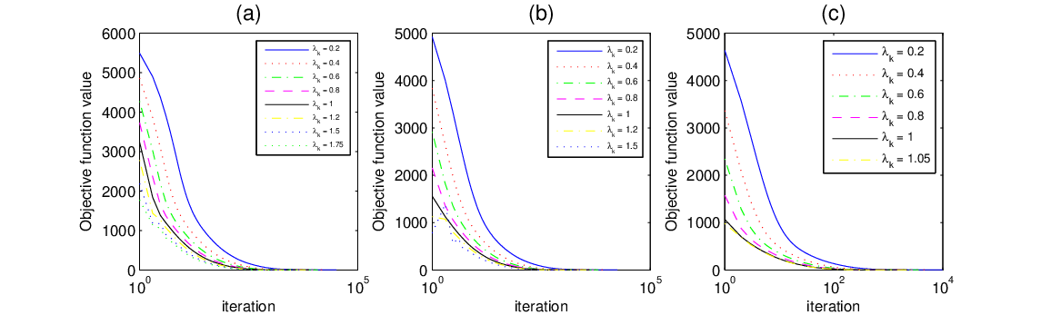
Refer to caption
Figure 1: The objective function value against the number of iterations for the LASSO problem. (a) γk=12​L\gamma_{k}=\frac{1}{2L}, (b) γk=1L\gamma_{k}=\frac{1}{L} and (c) γk=1.9L\gamma_{k}=\frac{1.9}{L}.
Refer to caption
Figure 2: The recovered sparse signal versus the true kk-sparse signal.

6 Conclusions

In this paper, we proposed a new convergence analysis of the variable metric forward-backward splitting algorithm (1.7) with extended relaxation parameters. Based on the averaged operator Jγk​Uk​A​(I−γk​Uk​B)J_{\gamma_{k}U_{k}A}(I-\gamma_{k}U_{k}B) and the firmly nonexpansive Jγk​Uk​AJ_{\gamma_{k}U_{k}A} on the Hilbert spaces HUk−1H_{U_{k}^{-1}}, we proved the weak convergence of this algorithm. Compared to existing work, we imposed a slightly weak condition on the relaxation parameters to ensure the convergence of the forward-backward splitting algorithm when using the variable metric and variable step sizes. Our results complemented and extended the corresponding results of Combettes and Yamada [8]. Furthermore, we obtained several general iterative algorithms for solving the variational inequality problem, the constrained convex minimization problem, and the split feasibility problem, respectively. These results generalized and improved the known results in the literature. Numerical experimental results on LASSO problem showed that the step size γk\gamma_{k} and relaxation parameter λk\lambda_{k} had much impact on the convergence speed of the proposed iterative algorithm. The larger the step size, the faster the algorithm converged. The over-relaxation parameter λk\lambda_{k} (λk>1\lambda_{k}>1) performed better than the under-relaxation parameter λk\lambda_{k} (λk≤1\lambda_{k}\leq 1).

Acknowledgement

This work was supported by the National Natural Science Foundations of China (11661056, 11771198, 11401293), the Postdoctoral Research Foundation of China (2015M571989) and the Postdoctoral Science Foundation of Jiangxi Province (2015KY51).

Conflict of interest

The authors declare no conflict of interest.

References

  • [1] P.L. Lions and B. Mercier. Splitting algorithms for the sum of two nonlinear operators. SIAM J. Numer. Anal., 16(6):964–979, 1979.
  • [2] George H.G. Chen and R.T. Rockafellar. Convergence rates in forward-backward splitting. SIAM J. Optim., 7(2):421–444, 1997.
  • [3] P. Tseng. A modified forward-backward splitting method for maximal monotone mappings. SIAM J. Control Optim., 38(2):431–446, 2000.
  • [4] P.L. Combettes. Solving monotone inclusions via compositions of nonexpansive averaged operators. Optimization, 53:475–504, 2004.
  • [5] G. Lopez, V. Martin-Marquez, F. Wang, and H.K. Xu. Forward-backward splitting method for accretive operators in banach spaces. Abstr. Appl. Anal., 2012(Article ID 109236):25 pages, 2012.
  • [6] C. Zong, Y.T. Tang, Y.J. Cho. Convergence analysis of an inexact three-operator splitting algorithm. Symmetry, 10:563, 2018.
  • [7] H.W. Jiao and F.H. Wang. On an iterative method for finding a zero to the sum of two maximal monotone operators. J. Appl. Math., 2014(414031):1–5, 2014.
  • [8] P.L. Combettes and I. Yamada. Compositions and convex combinations of averaged nonexpansive operators. J. Math. Anal. Appl., 425:55–70, 2015.
  • [9] H.H. Bauschke and P.L. Combettes. Convex Analysis and Motonone Operator Theory in Hilbert Spaces. Springer, London, second edition, 2017.
  • [10] A. Beck and M. Teboulle. A fast iterative shrinkage-thresholding algorithm for linear inverse problems. SIAM J. Imaging Sci., 2:183–202, 2009.
  • [11] A. Beck and M. Teboulle. Fast gradient-based algorithms for constrained total variation image denoising and deblurring problems. IEEE Trans. Image Process., 18(11):2419–2434, 2009.
  • [12] J.F. Cai, E.J. Candes, and Z. Shen. A singular value thresholding algorithm for matrix completion. SIAM J. Optim., 20:1956–1982, 2010.
  • [13] P.L. Combettes and V.R. Wajs. Signal recovery by proximal forward-backward splitting. Multiscale Model. Simul., 4:1168–1200, 2005.
  • [14] P. L. Combettes and J.C. Pesquet. Primal-dual splitting algorithm for solving inclusions with mixtures of composite, lipschitzian, and parallel-sum type monotone operators. Set-Valued Var. Anal., 20(2):307–330, 2012.
  • [15] B.C. Vũ. A splitting algorithm for dual monotone inclusions involving cocoercive operators. Adv. Comput. Math., 38:667–681, 2013.
  • [16] E. Esser, X. Zhang, and T. Chan. A general framework for a class of first order primal-dual algorithms for convex optimization in imaging science. SIAM J. Imaging Sci., 3(4):1015–1046, 2010.
  • [17] A. Chambolle and T. Pock. A first-order primal-dual algorithm for convex problems with applications to imaging. J. Math. Imaging Vision, 40(1):120–145, 2011.
  • [18] J.V. Burke and M.J. Qian. A variable metric proximal point algorithm for monotone operators. SIAM J. Control Optim., 37(2):353–375, 1998.
  • [19] L.A. Parente, P.A. Lotito, and M.V. Solodov. A class of inexact variable metric proximal point algorithms. SIAM J. Optim., 19(1):240–260, 2008.
  • [20] B.S. He and X.M. Yuan. Convergence analysis of primal-dual algorithms for a saddle-point problem: from contraction perspective. SIAM J. Imaging Sci., 5(1):119–149, 2012.
  • [21] B.C. Vũ. A variable metric extension of the forward-backward-forward algorithm for monotone operators. Numer. Funct. Anal. Optim., 34(9):1050–1065, 2013.
  • [22] J. Liang. Convergence rates of first-order operator splitting methods. PhD thesis, 2016.
  • [23] S. Bonettini, F. Porta, and V. Ruggiero. A variable metric forward-backward method with extrapolation. SIAM J. Sci. Comput., 38(4):A2558–A2584, 2016.
  • [24] P.A. Lotito, L.A. Parente, and M.V. Solodov. A class of variable metric decomposition methods for monotone variational inclusions. J. Convex Anal., 16:857–880, 2009.
  • [25] P.L. Combettes and B.C. Vũ. Variable metric forward-backward splitting with applications to monotone inclusions in duality. Optimization, 63(9):1289–1318, 2014.
  • [26] M. Simoes. On some aspects of inverse problems in image processing. PhD thesis, 2017.
  • [27] H.H. Bauschke and P.L. Combettes. Convex Analysis and Motonone Operator Theory in Hilbert Spaces. Springer, London, 2011.
  • [28] J.J. Moreau. Fonctions convexes duales et points proximaux dans un espace hilbertien. C. R. Acad. Sci., Paris Ser. A Math, 255:2897–2899, 1962.
  • [29] C. Byrne. A unified treatment of some iterative algorithms in signal processing and image reconstruction. Inverse Probl., 20(1):103–120, 2004.
  • [30] N. Ogura and I. Yamada. Non-strictly convex minimization over the fixed point set of the asymptotically shrinking nonexpansive mapping. Numer. Funct. Anal. Optim., 23:113–137, 2002.
  • [31] P.L. Combettes and V.R. Wajs. Variable metric quasi-fejer monotonicity. Nonlinear Anal., 78:17–31, 2013.
  • [32] Y. Censor and T. Elfving. A multiprojection algorithm using bregman projections in a product space. Numer. Algorithms, 8:221–239, 1994.
  • [33] H.K. Xu. A variable krasnoselskii-mann algorithm and the multiple-set split feasibility problem. Inverse Probl., 22:2021–2034, 2006.
  • [34] H.K. Xu. Iterative methods for the split feasibility problem in infinite dimensional hilbert spaces. Inverse Probl., 26:105018(17pp), 2010.
  • [35] Q. Yang and J. Zhao. Generalized km theorems and their applications. Inverse Probl., 22:833–844, 2006.
  • [36] H.K. Xu. Averaged mappings and the gradient-projection algorithm. J. Optim. Theory Appl., 150:360–378, 2011.
  • [37] R. Tibshirani. Regression shrinkage and selection via the LASSO. J. R. Stat. Soc. Ser. B Stat. Methodol., 58:267–288, 1996.