Acknowledgments

Continuum Kinetic Simulations of Plasma Sheaths and Instabilities

Petr Cagas

Dissertation submitted to the Faculty of the

Virginia Polytechnic Institute and State University

in partial fulfillment of the requirements for the degree of

Doctor of Philosophy

Aerospace Engineering

Bhuvana Srinivasan, Chair

Colin S. Adams

Wayne A. Scales

Timothy Warburton

30 ${}^{\text{th}}$ July, 2018

Blacksburg, Virginia

Keywords: Plasma Sheath, Discontinuous Galerkin, Continuum Kinetic Method, Plasma Instabilities, Plasma-Material Interactions

Continuum Kinetic Simulations of Plasma Sheaths and Instabilities

Petr Cagas

(ABSTRACT)

A careful study of plasma-material interactions is essential to understand and improve the operation of devices where plasma contacts a wall such as plasma thrusters, fusion devices, spacecraft-environment interactions, to name a few. This work aims to advance our understanding of fundamental plasma processes pertaining to plasma-material interactions, sheath physics, and kinetic instabilities through theory and novel numerical simulations. Key contributions of this work include (i) novel continuum kinetic algorithms with novel boundary conditions that directly discretize the Vlasov/Boltzmann equation using the discontinuous Galerkin method, (ii) fundamental studies of plasma sheath physics with collisions, ionization, and physics-based wall emission, and (iii) theoretical and numerical studies of the linear growth and nonlinear saturation of the kinetic Weibel instability, including its role in plasma sheaths.

The continuum kinetic algorithm has been shown to compare well with theoretical predictions of Landau damping of Langmuir waves and the two-stream instability. Benchmarks are also performed using the electromagnetic Weibel instability and excellent agreement is found between theory and simulation. The role of the electric field is significant during nonlinear saturation of the Weibel instability, something that was not noted in previous studies of the Weibel instability. For some plasma parameters, the electric field energy can approach magnitudes of the magnetic field energy during the nonlinear phase of the Weibel instability.

A significant focus is put on understanding plasma sheath physics which is essential for studying plasma-material interactions. Initial simulations are performed using a baseline collisionless kinetic model to match classical sheath theory and the Bohm criterion. Following this, a collision operator and volumetric physics-based source terms are introduced and effects of heat flux are briefly discussed. Novel boundary conditions are developed and included in a general manner with the continuum kinetic algorithm for bounded plasma simulations. A physics-based wall emission model based on first principles from quantum mechanics is self-consistently implemented and demonstrated to significantly impact sheath physics. These are the first continuum kinetic simulations using self-consistent, wall emission boundary conditions with broad applicability across a variety of regimes.

This research was supported by the Air Force Office of Scientific Research under grant number FA9550-15-1-0193.

The author acknowledges Advanced Research Computing at Virginia Tech for providing computational resources and technical support that have contributed to the results reported within this work. URL: http://www.arc.vt.edu

Continuum Kinetic Simulations of Plasma Sheaths and Instabilities

Petr Cagas

(GENERAL AUDIENCE ABSTRACT)

An understanding of plasma physics is vital for problems on a wide range of scales: from large astrophysical scales relevant to the formation of intergalactic magnetic fields, to scales relevant to solar wind and space weather, which poses a significant risk to Earth’s power grid, to design of fusion devices, which have the potential to meet terrestrial energy needs perpetually, and electric space propulsion for human deep space exploration. This work aims to further our fundamental understanding of plasma dynamics for applications with bounded plasmas. A comprehensive understanding of theory coupled with high-fidelity numerical simulations of fundamental plasma processes is necessary, this then can be used to improve improve the operation of plasma devices.

There are two main thrusts of this work. The first thrust involves advancing the state-of-the-art in numerical modeling. Presently, numerical simulations in plasma physics are typically performed either using kinetic models such as particle-in-cell, where individual particles are tracked through a phase-space grid, or using fluid models, where reductions are performed from kinetic physics to arrive at continuum models that can be solved using well-developed numerical methods. The novelty of the numerical modeling is the ability to perform a complete kinetic calculation using a continuum description and evolving a complete distribution function in phase-space, thus resolving kinetic physics with continuum numerics.

The second thrust, which is the main focus of this work, aims to advance our fundamental understanding of plasma-wall interactions as applicable to real engineering problems. The continuum kinetic numerical simulations are used to study plasma-material interactions and their effects on plasma sheaths. Plasma sheaths are regions of positive space charge formed everywhere that a plasma comes into contact with a solid surface; the charge inequality is created because mobile electrons can quickly exit the domain. A local electric field is self-consistently created which accelerates ions and retards electrons so the ion and electron fluxes are equalized. Even though sheath physics occurs on micro-scales, sheaths can have global consequences. The electric field accelerates ions towards the wall which can cause erosion of the material. Another consequence of plasma-wall interaction is the emission of electrons. Emitted electrons are accelerated back into the domain and can contribute to anomalous transport. The novel numerical method coupled with a unique implementation of electron emission from the wall is used to study plasma-wall interactions.

While motivated by Hall thrusters, the applicability of the algorithms developed here extends to a number of other disciplines such as semiconductors, fusion research, and spacecraft-environment interactions.

To my wife Kristýna and parents Kamila and Pavel

Acknowledgments

I consider myself extremely lucky to have many great people contributing to this work. The least I can do is to thank them all here.

First of all, I need to thank Dr. Kateřina Falk for pushing me out of my comfort zone and enabling all of this. I will be forever grateful to her for putting me in touch with my adviser and mentor, Professor Bhuvana Srinivasan.

And I could not have hoped for a better adviser. I think that her philosophy, that students need to be actively seeking help but then get all they want, works great for me. Her mentoring style resulted in me having a poster at APS DPP conference three months after joining the group. One of the things I will remember the most will be our evening discussions in front of the white-board in our office, which always reminded me why I love Physics. The only downside is that I was unable to grasp a concept of “sending email to the adviser to schedule a meeting” other students keep talking about.

And it still gets better because I did not have just one but two great advisers. Shortly after joining the group at VT, I met Dr. Ammar Hakim through a teleconference and he quickly became my second adviser in all but official title. When I first met him in person, he introduced himself to me and my colleagues as the person whom I was going to hate soon. Did not happen yet, though he got close when we were discussing color maps… Since my first week, we have been in contact on a daily basis discussing not just physics and programming but also politics and mad Richard Stallman. Ammar is also the reason why I ended up working on software engineering projects like making Conda builds of a code written mostly in Lua, compiled with LuaJIT, and relying heavily on automatically generated C code from Maxima.

Listening to other students, one can reach a conclusion that the sole purpose of the Graduate Committee is to make students cry during various meetings. My meetings were quite different because I always got an impression that the Committee members are genuinely interested in my work. What is more, I was interacting with them beyond the mandatory meetings. I was meeting Professor Colin Adams every Friday at our plasma physics Journal Club, which he organized. Using the expertise of Professor Wayne Scales about plasma waves resulted in him being a co-author of one of our publications. And last but not least, Professor Timothy Warburton provided a lot of valuable advice about the numerical aspects and his discontinuous Galerkin course has been in many aspects the best class I have ever taken.

Of course, I cannot forget my parents Kamila and Pavel who always supported me as much as they could. They made my growing up worriless, nurtured my curiosity, and shaped a great deal of who I am today. They only, for some mysterious reason, did not want me to pursue my musical talents but more on that later. When I was offered the opportunity to come to the States for the Ph.D., they gave me their unconditional support even though it must have been difficult for them. Without this support and the head start I got, I would never be able to achieve any of this work whatever my skills might be.

There are many other great people at VT who helped me stay steadily on top of all the necessary administrative requirements and were always very friendly to me. I would like to namely thank Rachel Hall Smith, Amy Burchett, Kelsey Wall, Jama Green, Cory Thompson, and Erin Wilson.

During my time at VT, many brilliant fellow students made their imprint on me. On the professional level, no other student had a bigger influence than Jimmy Juno. His report from a summer internship at PPPL helped me immensely to jump-start my research with Gkeyll. Since then, he has been always willing to discuss anything I needed help with (quite often it was the US comic book culture). When I joined the research group at VT, there were two other graduate students, Colin Glesner and Yang Song. I do not think I was suffering particularly bad from the culture shock but Colin Glesner was probably the one who helped me the most with the problems I had. Yang became the person sitting next to me in our office and that resulted in an interesting special relativity phenomenon. On many occasions, our casual office conversation ended after we realized it was suddenly many hours later and it was time to go home. As a senior grad student, Yang helped me professionally but also significantly broadened my cultural views. I have participated in the recruitment of Robert Masti, the Chair of our Beer Committee. After he joined our group, it did not take long to get to know him better and, nowadays, I like to think about him as ’murican brother. Special thanks also go to Jimmy and Chirag Rathod for reading this work and providing valuable comments. The rest of my group members which I did not name specifically, I would like to thank about staying cool with me during our group meeting. I hope they know my comments were always motivated by just the best intentions.

I also made some friends outside the department. Ashley Gates and Loren Brown became such good friends that we eventually moved right next to them. The process of moving was not simple and they went to great lengths to help us. A very special place belongs to Kiaya and Matthew Vincent who forced on us (without any pressure) one of the kittens they were fostering. Since then, our furry monster Binks walks over us at night, bites everything that sticks out over the edge of our bed, and preferentially sits on pages with some of my notes or derivations. Long story short, I have never regretted our decision to adopt him.

It is often said that grad students should have something to do apart from research in order to keep their sanity. I fell in love with Jethro Tull and that motivated me to start playing the flute.¹¹ 1 For people knowing me for a long time, this is probably the most surprising piece of information in this whole work. Originally, I was trying to learn just on my own using the Flute for Dummies book but then I met Ms. Elizabeth Crone from the Virginia Tech’s School of Performing Arts. With her, my learning pace drastically improved and I started discovering a world I barely knew there is. But more importantly, she made me smile every week. I vividly remember walking from one lesson smiling to myself even though our work was just rejected from the Physical Review Letters.

No, I did not forget about my wife, Kristýna.²² 2 http://phdcomics.com/comics/archive.php?comicid=870 One thing, I will say about her, is that she likes to make long-term plans. And still, she dropped everything and in three months went with me through the admission process, which usually takes foreigners at least a year. The fact that she was accepted to VT as well is one of the most amazing things that ever happened to me. She loves me, stays with me, and supports me as much as I need anywhere we are. Her I thank the most.

Chapter 1 Introduction

All models are wrong, but some are useful.

George E. P. Box

In the past few decades, numerical simulations have undergone rapid development and established themselves firmly as the third pillar of physics along with theory and experiment. To develop high-fidelity, carefully benchmarked numerical simulations, models need to be built from the bottom up, with each part tested rigorously.

This is especially important for complex problems requiring rich physics. One such example is the Hall thruster. These electrostatic plasma thrusters have been known for many decades and have been successfully flown on spacecraft; however, there are still gaps in our understanding of the underlying physics. Presently there are no global models with truly predictive capabilities because details of the electron transport inside the Hall thruster channel are not fully understood. This challenge extends to plasma devices and applications beyond Hall thrusters as well, where microscale physics can significantly affect macroscale phenomena and the subtle interplay remains an open research question.

The aim of this project is to leverage recent progress made in mathematics and software engineering to develop a new, self-consistent, physically-relevant model to advance our fundamental understanding of plasma physics for a number of applications. As a result, this work constitutes a complementary blend of physics, mathematics, and software engineering.

1.1 Plasma and Hall Thrusters

Hall thrusters (HT; also called Stationary Plasma Thrusters or deceivingly Hall Effect Thrusters¹¹ 1 When a linear conductor is put into magnetic field perpendicular to current flowing inside, Lorentz force deflects the flow and eventually leads to charging of its edges. Created electric field then accelerates particles in the opposite direction, effectively countering the effect of the magnetic field. This is called the Hall effect and, since magnetic field plays a crucial role in Hall thrusters, Hall effect needs to be avoided; this is the reason why Hall thrusters are circular rather than linear (Boeuf, 2017).) are a type of electric propulsion which was invented in the 1960s and first flown on the Soviet satellite Meteor-18 on 29 December 1971 (Morozov, 2003). Meteor-18 was a $15\text{\,}\mathrm{t}$ satellite and the HT, developed at the Kurchatov Institute of Atomic Energy, managed to lift the spacecraft by $15\text{\,}\mathrm{k}\mathrm{m}$ in a week, orient it, and maintain the orbital altitude. In the following years, Soviets and later Russians launched many more satellites with HT on board, while in the U.S., the development focused on an alternative electric propulsion concept: gridded ion thrusters. Hall thrusters were first used in Europe and the States in the 1990s.

Nowadays, HTs are still mainly used for altitude keeping, but are also considered as a type of propulsion for deep space journeys. In other words, they are used for purposes where classical chemical propulsion is lacking. While chemical propulsion is essential for high thrust missions, like launches into orbit, it presents serious constrains for traveling beyond Mars. An unavoidable problem for most propulsion concepts²² 2 Concepts like solar sails or experimental work like White et al. (2016) are not discussed in this work. is the need to accelerate the remaining propellant together with the useful payload. This is demonstrated by the ideal rocket equation,

\displaystyle\Delta v=c_{e}\mathrm{ln}\,\left(\frac{m_{0}}{m_{f}}\right),

(1.1)

where $\Delta v$ is the measure of an impulse needed for the mission, $c_{e}$ is the effective exhaust velocity, $m_{0}$ and $m_{f}$ are the initial and final masses of the spacecraft, respectively. Instead of the exhaust velocity, it is common to use specific impulse, $I_{sp}=c_{e}/g_{0}$ , where $g_{0}$ is Earth’s gravitational acceleration, which can be seen as a measure of fuel efficiency. The mass ratio then follows

\displaystyle\frac{m_{0}}{m_{f}}=\exp\left(\frac{\Delta v}{I_{sp}g_{0}}\right).

For example, a mission defined by $\Delta v=$11\,186\text{\,}\mathrm{m}\,\mathrm{s}^{-1}$$ (Earth escape $\Delta v$ ) and a propulsion system with $I_{sp}\approx$400\text{\,}\mathrm{s}$$ , which is a reasonable $I_{sp}$ for chemical propulsion, has the mass ratio around 18. The ratio gets even worse for more extreme missions. Getting $10\text{\,}\mathrm{k}\mathrm{g}$ of useful payload to the nearest star from the Sun (around 5 light years) in $5000\text{\,}\mathrm{y}\mathrm{e}\mathrm{a}\mathrm{r}\mathrm{s}$ using a propulsion system with $I_{SP}=$500\text{\,}\mathrm{s}$$ requires fuel which is on the order of the Earth mass ( $5.972\text{\times}{10}^{24}\text{\,}\mathrm{k}\mathrm{g}$ (Luzum et al., 2011)). Clearly, the mass ratio can be improved by increasing specific impulse, $I_{sp}$ . For chemical propulsion, the source of the energy are chemical bonds in the propellant. This energy is used to increase the enthalpy of the propellant which is subsequently converted into kinetic energy with a nozzle. Therefore, the specific impulse of chemical propulsion is limited, unless a radically new propellant is found. On the other hand, electrostatic propulsion³³ 3 Other types of the electric propulsion (e.g., arc-jets and resistojets) heat the propellant electrically and then follow same principles like the chemical propulsion. Electromagnetic propulsion concepts use the Lorentz force. However, these are not considered for this work. uses an electrostatic field to accelerate ionized propellant; therefore, the exhaust velocity is variable and can be calculated with

\displaystyle c_{e}=\sqrt{\frac{2q\phi}{m}},

where $q$ and $m$ are the propellant charge and mass, and $\phi$ is the applied electrostatic potential. In theory, the propellant could be accelerated to an indiscriminately high velocity. However, new constraints posed by electric propulsion, due to needing a power source, increase the overall mass of the system and prohibit an unlimited acceleration. Despite the aforementioned limitation, up to ten-fold higher $I_{sp}$ of electric propulsion systems allows them to maintain a better fuel efficiency compared to chemical propulsion.

Hall thrusters span a wide part of the propulsion parameter space. Currently, their power ranges from $100\text{\,}\mathrm{W}$ to $30\text{\,}\mathrm{k}\mathrm{W}$ , across a variety of sizes, with $I_{sp}$ up to $3000\text{\,}\mathrm{s}$ , and thrust between mN and N (Boeuf, 2017). Additional concepts, like nested HTs or arrays of HTs are constitute current research (Hall et al., 2017), as the amount of available power on satellites increases.

The basic principle of HTs is simple. Neutral gas gets ionized and is then accelerated by an electrostatic field. However, maintaining the external electric field is challenging due to the complexity of the plasma⁴⁴ 4 It is not without interest, that the name “plasma” was first used by Langmuir around 1927 because it reminded him how blood plasma (electron fluid) carries corpuscles (ions). created inside.

In popular literature, plasma is referred to as a fourth state of matter, obtained when electrons leave their atoms. This classification is, however, questionable since the ionization ratio can vary and there is no clear distinction between plasma and neutral gas, like it is with the other states of matter. A proper definition is more complicated:

Plasma is a quasi-neutral mixture of electrons, ions, and neutral atoms and molecules in various quantum states which exhibit collective behavior.

Particularly, the last point of the definition is very important. The electrons in a plasma have much higher mobility that the other species due to their low mass (in the simplest hydrogen plasma, the mass ratio between electrons and ions is $\approx$ 1836) and can rearrange themselves to shield an external electric field. Considering a simplified case of a 1D hydrogen plasma with a potential $\phi$ , Poisson’s equation gives

\displaystyle\nabla^{2}\phi=-\frac{q_{i}n_{i}-q_{e}n_{e}}{\varepsilon_{0}},

(1.2)

where $n_{e}$ and $n_{i}$ are electron and ion number densities and $\varepsilon_{0}$ is the vacuum permitivity. It can be assumed that on time-scales relevant to electrons, ions retain the density unperturbed by the electric field, i.e., $n_{i}=n_{0}$ . The particle distribution function of electrons is (see Chapter 2 for more details on distribution functions)

\displaystyle f_{e}(x,\,v_{x})=A\exp\left(-\frac{\frac{1}{2}m_{e}v_{x}^{2}+q_{e}\phi}{T_{e}}\right),

(1.3)

where $A$ is some normalization constant and $T_{e}$ is the electron temperature (in eV). Integrating Eq. (1.3) over $v_{x}$ leads to

\displaystyle n_{e}(x)=n_{0}\exp\left(-\frac{q_{e}\phi(x)}{T_{e}}\right).

(1.4)

Substitution into the Poisson’s equation (Eq. 1.2) gives

\displaystyle\frac{d^{2}\phi}{dx^{2}}=\frac{\mathrm{e}n_{0}}{\varepsilon_{0}}\left[\exp\left(-\frac{q_{e}\phi}{T_{e}}\right)-1\right].

The small argument Taylor series expansion is then used to obtain

\displaystyle\frac{d^{2}\phi}{dx^{2}}=\frac{q_{e}n_{0}}{\varepsilon_{0}}\frac{q_{e}\phi}{T_{e}}.

The solution to this differential equation is

\displaystyle\phi=\phi_{0}\exp\left(-\frac{|x|}{\lambda_{D}}\right),

where

\displaystyle\lambda_{D}=\sqrt{\frac{\varepsilon_{0}T_{e}}{n_{e}q_{e}^{2}}}

(1.5)

is a characteristic scale length called the Debye length. For a special case of a particle source with charge $q$ , the potential as a function of the distance $r$ follows

\displaystyle\phi(r)=\frac{1}{4\pi\varepsilon_{0}}\frac{q}{r}\exp\left(-\frac{r}{\lambda_{D}}\right).

This brings an important insight. In a plasma, electrons collectively rearrange themselves so the potential caused by a test particle is shielded and drops exponentially with a scale length of $\lambda_{D}$ , rather than as $\sim\frac{1}{r}$ . Getting back to the definition, quasi-neutrality can now be better described. In a plasma, the sum of the charges over a region much bigger than the volume corresponding to the Debye length is zero.

Therefore, an electric field cannot be simply used to accelerate particles in plasma, because electrons would simply rearrange themselves to shield the external field. There are a couple of solutions. Gridded ion thrusters, which were mentioned at the beginning, have a (sometimes called screening) grid, which is adjacent to the region where the plasma is generated, extracting ions. These ions are then accelerated by an electric field formed between the extractor grid and additional accelerator grid. The accelerating electric field, therefore, lies entirely outside of the plasma.

Hall thrusters implement a different approach. The plasma is located within an annulus with radial magnetic field formed by inner and outer magnetic coils and a magnetic circuit. The radial magnetic field decreases the mobility of electrons which follow the axial field. Consequently, the axial electric field does not get shielded even though it lies directly in the plasma region.

Even though HTs clearly work and have been flown in the real space environments, many of their aspects are not yet fully understood. Boeuf (2017) lists these three main reasons:

1.

The magnetic barrier perpendicular to the cathode-anode flow can be subject to a variety of instabilities which can significantly decrease the electron confinement.
2.

Electron interactions with the wall result in electron emissions which alter electron transport and plasma in general.
3.

Neutral gas needs to by highly ionized for good extraction. Ionization also introduces additional oscillatory modes like the breathing mode.

A wide range of numerical simulations exist for HTs, however, first principles computations to self-consistently evolve all aspects of a Hall thruster have yet to be performed. A common practice is to implement empirically-determined estimates of electron mobility inside the channel into the simulation (Koo and Boyd, 2006).

1.2 Plasma Simulations

There are two classical approaches to plasma simulation: particle methods and fluid methods.

The first approach directly evolves positions and velocities using equations of motion with electromagnetic forces. A natural way to obtain the forces is to apply the principle of superposition on interactions between the individual particles. For example in an electrostatic case, the interactions are given by the Coulomb force,

\displaystyle\bm{F}_{AB}=\frac{1}{4\pi\varepsilon_{0}}\frac{q_{A}q_{B}}{r_{AB}^{3}}\bm{r}_{AB}.

(1.6)

The infinite range of electromagnetic forces requires all the particle pairs to be accounted for; which makes for an expensive algorithm, $\mathcal{O}(N^{2})$ , where $N$ is the number of particles. A more efficient method is to interpolate all the particles on a mesh of grid points and calculate the electromagnetic forces on the mesh using Poisson’s equation and Ampere’s law. The forces are then interpolated back onto particle positions in neighboring grid cells. In comparison to the naive approach, this algorithm significantly decreases the computational cost to $\mathcal{O}(N\mathrm{log}N)$ . The strength of this method is that no assumptions about the particle dynamics are made and, therefore, a wide variety of kinetic phenomena is intrinsically included in the system. This makes particle methods particularly well suited for simulation of weakly collisional plasmas where particle distributions are far from the equilibrium.

On the other hand, particle methods theoretically require simulating unfeasible amount of particles.⁵⁵ 5 Munroe (2014) provides a charming description of the magnitude of the numbers involve. One mol of a gas at standard condition has a volume of $22.4\text{\,}\mathrm{d}\mathrm{m}^{3}$ , which is an imaginable amount. Such a volume contains the Avogadro’s number, $\mathrm{N}_{A}=6.022\times 10^{23}$ , of particles. Munroe (2014) asks a question, “How big would a mol of moles be?”, by which he means the Avogadro’s number of moles. He estimates that the amount would cover the Earth surface up to couple tens of kilometers or form a compact body of a size of the Moon. Instead, individual particles are grouped into a fewer number of “macro-particles,” which decreases computational cost but also introduces statistical noise. The noise can be decreased by increasing the number of “macro-particles,” however, the signal-to-noise ratio improves only as $\sqrt{N}$ , where $N$ is the number of particles per grid cell, which makes this an inefficient proposition.

In a situation where temporal and spatial scales of gyromotion⁶⁶ 6 Circular motion of charged particles around the magnetic field lines. are much shorter than the scale of interest, the system can be reduced by integrating over one velocity component. This approach is called gyro-kinetics.

The system of equations can be reduced even more by integration over the two remaining velocity components, which leads to the fluid description of the plasma. In the fluid model, the individual particle positions and velocities are lost and only the macroscopic quantities like density, $n$ or bulk velocity, $\bm{u}$ , are resolved. These are resolved by evolving the conservation equations; for example the continuity equation (see Sec. 2.3 for more information),

\displaystyle\frac{\partial n}{\partial t}+\nabla\cdot(n\bm{u})=0.

Fluid models are excellent tools for macroscopic plasma simulation, because they are usually a couple of orders of magnitude faster than kinetic models and are not affected by statistical noise. However, any kinetic effects that may be potentially relevant for a given situation need to be artificially included.

This work focuses on an alternative approach – a continuum kinetic method which relies on directly discretizing the Vlasov equation (see Chapter 2 for more details),

\displaystyle\frac{\partial f}{\partial t}+\bm{v}\cdot\nabla_{\bm{x}}f+\frac{q}{m}\left(\bm{E}+\bm{v}\times\bm{B}\right)\cdot\nabla_{\bm{v}}f=0,

where $f$ is the particle distribution. Having a similar mathematical form as other conservation equations, the same approach can be used to solve it, e.g., finite-elements methods. However, since the distribution function $f$ is directly discretized, no assumptions over the individual particle velocities are necessary. In other words, continuum kinetic methods provide noise-free solutions with kinetic effects intrinsically included in the system.

1.3 Objectives

The goal of this work is to build and test model pieces necessary to create a truly predictive Hall thruster model and provide a better understanding of plasma-material interactions. The model is intended to be applicable to a variety of plasma configurations. The objectives can be further specified as

1.

Develop a continuum kinetic framework to study plasma sheath physics and benchmark this framework to studies of plasma instabilities.
2.

Increase the fidelity of classical sheath simulations by accounting for additional physics brought about through appropriate collision operators and ionization.
3.

Understand plasma-material interactions in Hall thrusters by developing a secondary electron emission boundary condition based on phenomenological models to study its effect on sheaths. Particularly test possible changes to the shape of the sheath potential based on the emission and collisions. Also, an understanding of secondary electron emission (SEE) using a kinetic model can provide insight into fluid boundary conditions to appropriately model SEE.

1.4 Notes on Conventions Used

The International System of Units (SI; Système international d’unités) is used throughout the work with the exception of temperature, which is given in terms of energy, i.e., it is assumed to by multiplied by the Boltzmann constant, $k_{\mathrm{B}}=$1.380\,648\,52(79)\text{\times}{10}^{-23}\text{\,}\mathrm{J}\mathrm{/}\mathrm{K}$$ (Mohr et al., 2016). What is more, it is common in plasma physics to use electron-volts as a unit of energy instead of Joules, $1\text{\,}\mathrm{e}\mathrm{V}$=$1.602\,176\,62\text{\times}{10}^{-19}\text{\,}\mathrm{J}$ .

Einstein’s summation convention is used for the tensor indices. For example, if $\mathbf{a}=\left(a_{1},a_{2},a_{3}\right)$ and $\mathbf{b}=\left(b_{1},b_{2},b_{3}\right)$ ,

\displaystyle a_{i}b_{i}=\sum_{i}^{3}a_{i}b_{i}=a_{1}b_{1}+a_{2}b_{2}+a_{3}b_{3}.

Another good example is with the Levi-Civita symbol, $\varepsilon_{ijk}$ ,

\displaystyle\varepsilon_{1jk}a_{j}b_{k}=a_{2}b_{3}-a_{3}b_{2}.

1.5 Notes on the Simulations

The numerical development, simulations, and post-processing in this work are performed using the Gkeyll framework and this work has contributed to core development of Gkeyll.⁷⁷ 7 http://gkeyll.readthedocs.io/en/latest/ Gkeyll 2.0 is used as the simulation tool of choice for this work.

In order to provide the maximum reproducibility of the presented results, all simulation initialization files are available for the reader together with the details of some postprocessing techniques. Gkeyll 2.0 build is available in the Anaconda cloud and can be conveniently installed using the conda package manager⁸⁸ 8 Installing Gkeyll 2.0 through conda most likely results in suboptimal performance, however, it is useful for experimentation on a new machine. Production level run should use properly built code utilizing local message parsing interface (MPI).

⬇

1 conda install -c gkyl gkyl

Assuming Anaconda is already in the PATH, the simulations can then be run, for example with

⬇

1 gkyl two-stream.lua

Chapter 2 Numerical Model and Implementation

An approximate answer to the right problem is worth a good deal more than an exact answer to an approximate problem.

John Turkey

This chapter describes kinetic plasma equations; both the analytic derivation of the governing Vlasov/Boltzmann equations and its numerical discretization. The fluid approximation is discussed as well.

2.1 Kinetic Plasma Equation

The word kinetic originates from the ancient Greek kinein which means to move. Nowadays, Merriam-Webster dictionary defines it as of or relating to the motion of material bodies and the forces and energy associated therewith. In physics, kinetic means that the motions of individual particles or macro-particles are taken into account and no assumption on the velocity distribution is done a priori.

2.1.1 Klimontovich Equation

Nicholson (1983) starts the derivation of the full kinetic theory with a definition of a density of a single particle, $i$ ,

\displaystyle N_{i}(t,\bm{x},\bm{v})=\delta\big(\bm{x}-\bm{X}_{i}(t)\big)\delta\big(\bm{v}-\bm{V}_{i}(t)\big),

where $\delta$ is the Dirac delta function and $\bm{X}$ and $\bm{V}$ are the Lagrangian coordinates of the particle. Note that, even though the function is nonzero only at the position of the particle, it is defined over the whole phase space, i.e., the 6-dimensional space which is a combination of the 3-dimensional configuration space (parameterized with $\bm{x}$ ) and 3-dimensional velocity space (parameterized by $\bm{v}$ ). In other words, the location in phase space provides not only the information about the physical position but also the vector of velocity. Consequently, the units of $N$ are $\mathrm{m}^{-6}\mathrm{s}^{3}$ rather than $\mathrm{m}^{-3}$ used for the classical density.

The extension for multiple particles is then obtained as a summation over the individual densities

\displaystyle N_{s}(t,\bm{x},\bm{v})=\sum_{i}\delta\big(\bm{x}-\bm{X}_{i}(t)\big)\delta\big(\bm{v}-\bm{V}_{i}(t)\big).

(2.1)

From now on, the index $s$ will denote the type of the particles, i.e., electrons, ions, etc.

The description of this distribution is not of particular interest. For the purposes of the kinetic theory, the information about the evolution of the system based on the current state is more intriguing. Therefore, we proceed with taking the time derivative of Eq. (2.1),

\displaystyle\begin{aligned} \frac{\partial N_{s}(t,\bm{x},\bm{v})}{\partial t}=&-\sum_{i}\bm{\dot{X}}_{i}\cdot\nabla_{\bm{x}}\delta\big(\bm{x}-\bm{X}_{i}(t)\big)\delta\big(\bm{v}-\bm{V}_{i}(t)\big)\\ &-\sum_{i}\bm{\dot{V}}_{i}\cdot\nabla_{\bm{v}}\delta\big(\bm{x}-\bm{X}_{i}(t)\big)\delta\big(\bm{v}-\bm{V}_{i}(t)\big),\end{aligned}

(2.2)

where $\nabla_{\bm{x}}=(\partial_{x},\partial_{y},\partial_{z})$ and $\nabla_{\bm{v}}=(\partial_{v_{x}},\partial_{v_{y}},\partial_{v_{z}})$ .

Up until this point, the whole description was purely mathematical. Now it is required to include physics; specifically the relation

\displaystyle\bm{\dot{X}}_{i}(t)=\bm{V}_{i}(t)

(2.3)

and the Lorentz force equation

\displaystyle m_{s}\bm{\dot{V}}_{i}=q_{s}\bm{E}^{m}\big(t,\bm{X}_{i}(t)\big)+q_{s}\bm{V}_{i}(t)\times\bm{B}^{m}\big(t,\bm{X}_{i}(t)\big),

(2.4)

where $m_{s}$ and $q_{s}$ are mass and charge respectively of particle $s$ . $\bm{E}^{m}$ and $\bm{B}^{m}$ represent microscopic electric and magnetic fields from other particles (fields from the particle itself are neglected) together with the external macroscopic fields. The microscopic fields satisfy Maxwell’s equations,

$\displaystyle\nabla\cdot\bm{E}^{m}(t,\bm{x})$	$\displaystyle=\frac{\rho^{m}(t,\bm{x})}{\varepsilon_{0}},$	(2.5)
$\displaystyle\nabla\cdot\bm{B}^{m}(t,\bm{x})$	$\displaystyle=0,$	(2.6)
$\displaystyle\nabla\times\bm{E}^{m}(t,\bm{x})$	$\displaystyle=-\frac{\partial\bm{B}^{m}(t,\bm{x})}{\partial t},$	(2.7)
$\displaystyle\nabla\times\bm{B}^{m}(t,\bm{x})$	$\displaystyle=\mu_{0}\bm{j}^{m}(t,\bm{x})+\mu_{0}\varepsilon_{0}\frac{\partial\bm{E}^{m}(t,\bm{x})}{\partial t},$	(2.8)

where $\rho^{m}$ is microscopic charge density

\displaystyle\rho^{m}(t,\bm{x})=\sum_{s}q_{s}\int N_{s}(\bm{x},\bm{v},t)\,d\bm{v}

and $\bm{j}^{m}$ is microscopic current density (surface density, $[j]=$\mathrm{A}\,\mathrm{m}^{-2}$$ )

\displaystyle\bm{j}^{m}(t,\bm{x})=\sum_{s}q_{s}\int\bm{v}N_{s}(\bm{x},\bm{v},t)\,d\bm{v}.

Substituting Eq. (2.3) and Eq. (2.4) into the evolution equation (Eq. 2.2) gives

	$\displaystyle\frac{\partial N_{s}(t,\bm{x},\bm{v})}{\partial t}=$	$\displaystyle-\sum_{i}\bm{V}_{i}\cdot\nabla_{\bm{x}}\delta\big(\bm{x}-\bm{X}_{i}(t)\big)\delta\big(\bm{v}-\bm{V}_{i}(t)\big)$
		$\displaystyle-\sum_{i}\frac{q_{s}}{m_{s}}\left[\bm{E}^{m}\big(t,\bm{X}_{i}(t)\big)+\bm{V}_{i}(t)\times\bm{B}^{m}\big(t,\bm{X}_{i}(t)\big)\right]\cdot\nabla_{\bm{v}}\delta\big(\bm{x}-\bm{X}_{i}(t)\big)\delta\big(\bm{v}-\bm{V}_{i}(t)\big).$

Using the property of the Dirac delta function, $a\delta(a-b)=b\delta(a-b)$ , $\bm{X}$ and $\bm{V}$ can be replaced with $\bm{x}$ and $\bm{v}$ and then the order of the summations and the gradients can be switched,

	$\displaystyle\frac{\partial N_{s}(t,\bm{x},\bm{v})}{\partial t}=$	$\displaystyle-\bm{v}\cdot\nabla_{\bm{x}}\sum_{i}\delta\big(\bm{x}-\bm{X}_{i}(t)\big)\delta\big(\bm{v}-\bm{V}_{i}(t)\big)$
		$\displaystyle-\frac{q_{s}}{m_{s}}\left[\bm{E}^{m}\big(t,\bm{x}\big)+\bm{v}\times\bm{B}^{m}\big(t,\bm{x}\big)\right]\cdot\nabla_{\bm{v}}\sum_{i}\delta\big(\bm{x}-\bm{X}_{i}(t)\big)\delta\big(\bm{v}-\bm{V}_{i}(t)\big).$

Finally, density Eq. (2.1) can be back-substituted to obtain the Klimontovich equation,

\displaystyle\frac{\partial N_{s}(t,\bm{x},\bm{v})}{\partial t}+\bm{v}\cdot\nabla_{\bm{x}}N_{s}+\frac{q_{s}}{m_{s}}\left(\bm{E}^{m}+\bm{v}\times\bm{B}^{m}\right)\cdot\nabla_{\bm{v}}N_{s}=0.

(2.9)

Knowing the initial positions, $\bm{X}_{i}(t=0)$ , and velocities, $\bm{V}_{i}(t=0)$ , of all the particles, the Klimontovich equation (Eq. 2.9) together with Maxwell’s equations provides the full, exact description of the evolution of the plasma.

2.1.2 Vlasov/Boltzmann Equation

While the Klimontovich equation (Eq. 2.9) captures the discrete nature of individual particles exactly, the collection of Dirac Delta functions is not well suited for practical use. Therefore, we introduce a new smooth distribution function $f_{s}(t,\bm{x},\bm{v})$ , which is defined as

\displaystyle f_{s}(\bm{x},\bm{v},t):=\left\langle N_{s}(\bm{x},\bm{v},t)\right\rangle,

where $\langle\cdot\rangle$ denotes the ensemble average, i.e., an average over the all possible microstates realizing the given macro-state. This new distribution is the key variable of the continuum kinetic method and represents the phase space particle density integrated over the small volume $\Delta\bm{x}\Delta\bm{v}$ with center at $(\bm{x},\bm{v})$ . Analogously to the distribution $f$ , the ensemble averages can be defined for the fields as $\bm{E}:=\langle\bm{E}^{m}\rangle$ and $\bm{B}:=\langle\bm{B}^{m}\rangle$ .

When the ensemble averages are substituted into the Klimontovich equation (Eq. 2.9), the Boltzmann equation is obtained,

\displaystyle\frac{\partial f_{s}}{\partial t}+\bm{v}\cdot\nabla_{\bm{x}}f_{s}+\frac{q_{s}}{m_{s}}\left(\bm{E}+\bm{v}\times\bm{B}\right)\cdot\nabla_{\bm{v}}f_{s}=\underbracket{-\frac{q_{s}}{m_{s}}\big\langle\left(\delta\bm{E}+\bm{v}\times\delta\bm{B}\right)\cdot\nabla_{\bm{v}}\delta N_{s}\big\rangle}_{\sum\left(\frac{\delta f_{s}}{\delta t}\right)},

(2.10)

where the residuals are defined as

	$\displaystyle\delta N_{s}(\bm{x},\bm{v},t)$	$\displaystyle=N_{s}(\bm{x},\bm{v},t)-f_{s}(\bm{x},\bm{v},t),$
	$\displaystyle\delta\bm{E}(\bm{x},\bm{v},t)$	$\displaystyle=\bm{E}^{m}(\bm{x},\bm{v},t)-\bm{E}(\bm{x},\bm{v},t),$

and

\displaystyle\delta\bm{B}(\bm{x},\bm{v},t)=\bm{B}^{m}(\bm{x},\bm{v},t)-\bm{B}(\bm{x},\bm{v},t).

Note that in this form, the Boltzmann equation (Eq. 2.10) is exact and the term on the right-hand-side of the equation captures the intrinsically discrete effects, such as collisions, but also effects like photo-ionization.

In a regime where discrete particle effects are negligible, Eq. (2.10) is reduced to the Vlasov equation, which is the center-piece of this work,

\displaystyle\frac{\partial f_{s}}{\partial t}+\bm{v}\cdot\nabla_{\bm{x}}f_{s}+\frac{q_{s}}{m_{s}}\left(\bm{E}+\bm{v}\times\bm{B}\right)\cdot\nabla_{\bm{v}}f_{s}=0.

(2.11)

It is worth noting that the Vlasov equation (Eq. 2.11) is not relativistic. The relativistic extension can be obtained by adding appropriate Lorentz factors, $\gamma$ ,

\displaystyle\frac{\partial f_{s}}{\partial t}+\nabla_{\bm{x}}\cdot\left(\frac{\bm{p}}{m_{s}\gamma}f_{s}\right)+\nabla_{\bm{p}}\cdot\left[q_{s}\left(\bm{E}+\frac{\bm{p}}{m_{s}\gamma}\times\bm{B}\right)f_{s}\right]=0,

(2.12)

where

\displaystyle\gamma=\frac{1}{\sqrt{1-\bm{p}^{2}/m_{s}^{2}c^{2}}}.

This work neglects relativistic effects.

2.1.3 Particle Distribution Function

An insight into what the distribution function represents is key to understanding many figures presented in this work. Configuration space plots are much more common in the scientific literature than phase space plots, hence a more in-depth discussion of distribution functions and phase space is warranted.

First, let us illustrate the behavior of the distribution function in phase space on a toy problem of collision-less neutral gas bouncing in a bounded domain, which is depicted in Fig. 2.1. The top left panel captures the initial condition – a collection of particles distributed around $x=0$ with a bulk (average) velocity of $u_{x}=1$ . Since the vast majority of particles have a positive velocity¹¹ 1 The thermal spread of particles follows the Gauss distribution so there are technically some particles with negative velocity, however, in this case the distribution has $\sigma=0.1$ . The region of negative velocities is farther than $10\,\sigma$ from the bulk velocity and is, therefore, negligible. the particles will propagate to the right (positive $x$ ). However, due to the thermal velocity spread, the distribution also becomes skewed. When the particles reach the wall at the right edge of the domain they are elastically reflected, i.e., the magnitude of the velocity is conserved but the sign (direction) is flipped. Noting that the normalized bulk velocity is 1 and the domain size is 10, it should be expected that exactly at $t=20$ the center of the distribution returns to the original position, which is seen in the bottom right panel of Fig. 2.1.

Refer to caption — Figure 2.1: Demonstration of the evolution of the particle distribution function in 2D phase space (1X1V). The top left panel captures the initial collection of particles with center at $x=0$ and with velocities thermally spread around $u_{x}=1$ . The other panels show evolution and elastic reflections from the walls at the edges of the domain. At the $t=20$ (bottom right panel) the center of the distribution returns to the original position. [Simulation input file: C.1]

Sometimes, it can be advantageous to integrate out the kinetic information in order get the macroscopic quantities -- moments of the distribution. The moments have the physical meaning of density, flux, energy, etc.²² 2 The distribution function used in this work is not multiplied by the mass and, therefore, the moments give the number density and flux rather than the mass density and momentum. The particle number density is obtained as the zeroth moment,

\displaystyle n(\bm{x})=\int_{\mathcal{V}}f(\bm{x},\bm{v})\,d\bm{v},

(2.13)

where the integration is performed over the entire velocity space, ${\mathcal{V}}$ . The first moment gives the particle flux,

\displaystyle n(\bm{x})\bm{u}(\bm{x})=\int_{\mathcal{V}}\bm{v}f(\bm{x},\bm{v})\,d\bm{v}.

(2.14)

Note that the moment gives the conserved variable, flux, rather than the primitive variable, bulk velocity. In order to obtain the primitive variables, the division by density is required,

\displaystyle\bm{u}(\bm{x})=\frac{\int_{\mathcal{V}}\bm{v}f(\bm{x},\bm{v})\,d\bm{v}}{\int_{\mathcal{V}}f(\bm{x},\bm{v})\,d\bm{v}}.

Note the similarity of the moment calculation to definition of an average value in statistical math; the average value of a variable $a$ with a probability distribution $p(a)$ is calculated as $\langle a\rangle=\int ap(a)\,da$ . However, while a probability is normalized to 1 and the distribution function here is normalized to $n$ .³³ 3 While this choice is common, there are works which normalize particle velocity distribution to 1 as well.

Finally, the second moment can be scaled to provide energy per unit mass. It can either be calculated as a scalar value of the total energy or as the energy tensor,

	$\displaystyle\mathcal{E}(\bm{x})$	$\displaystyle=\frac{1}{2}m\int_{\mathcal{V}}\|\bm{v}\|^{2}f(\bm{x},\bm{v})\,d\bm{v},$		(2.15)
	$\displaystyle\bm{\mathcal{E}}(\bm{x})$	$\displaystyle=\frac{1}{2}m\int_{\mathcal{V}}\bm{vv}f(\bm{x},\bm{v})\,d\bm{v},$		(2.16)

where $\bm{vv}$ is a dyadic tensor. The connection between the expressions is then $\mathcal{E}=\mathrm{Trace}(\bm{\mathcal{E}})$ .

While discussing the distribution functions, it is worth mentioning one which stands out in particular -- the Maxwellian distribution. Many textbooks provide the following derivation,⁴⁴ 4 This derivation is, apart from its simplicity, also of a historical interest because it is the argument originally given by Maxwell (1890). which assumes that the probability $f_{1D}(v_{x})dv_{x}$ , i.e. the probability of finding the particle in the interval $\langle v_{x},\,v_{x}+dv_{x}\rangle$ , is independent of $v_{y}$ and $v_{z}$ . Then

\displaystyle f(v_{x},v_{y},v_{z})dv_{x}dv_{y}dv_{z}=nf_{x}(v_{x})f_{y}(v_{y})f_{z}(v_{z})dv_{x}dv_{y}dv_{z}.

(2.17)

In a situation with no external forces, there is no preferred velocity direction and, therefore, the distribution must depend on the velocity only through its magnitude, $v_{x}^{2}+v_{y}^{2}+v_{z}^{2}$ . That means that

\displaystyle nf_{x}(v_{x})f_{y}(v_{y})f_{z}(v_{z})=f(v_{x},v_{y},v_{z})=F(v_{x}^{2}+v_{y}^{2}+v_{z}^{2}),

where $F$ is some unknown function. Solving the equation gives

\displaystyle f_{x}(v_{x})=A\exp(Bv_{x}^{2}),\quad f(v_{x},v_{y},v_{z})=nA^{3}\exp\big(B(v_{x}^{2}+v_{y}^{2}+v_{z}^{2})\big).

Then we can use the definitions of the moments to tie the integration constants $A$ and $B$ with the macroscopic physical quantities:

\displaystyle n=\int f\,d\bm{v}=\int nA^{3}\exp\big(-B(v_{x}^{2}+v_{y}^{2}+v_{z}^{2})\big)\,d\bm{v}\quad\Rightarrow\quad A=\sqrt{\frac{B}{\pi}}.

From the definition of the thermal velocity:⁵⁵ 5 The thermal velocity can be tied to the temperature through the Equipartition theorem, $NT/2=0.5mv_{th}^{2}$ , where $N$ is the number of degrees of freedom. It is worth noting, that this definition is not unique. For example, Chen (1985) ties thermal velocity and temperature for $N=1$ as $mv_{th}^{2}=2T$ , with gives Maxwellian distribution proportional to $\exp(-v_{x}^{2}/v_{th}^{2})$ . The advantage of the definition used in this work is (apart from satisfying the Equipartition theorem) that the Maxwellian distribution has the mathematical form of the normal distribution with thermal velocity being the variance, $\sigma$ .

\displaystyle v_{th}^{2}=\frac{1}{n}\int\bm{v}^{2}f\,d\bm{v}=\int(v_{x}^{2}+v_{y}^{2}+v_{z}^{2})\sqrt{\frac{B}{\pi}}^{3}\exp\big(-B(v_{x}^{2}+v_{y}^{2}+v_{z}^{2})\big)\,d\bm{v}\quad\Rightarrow\quad B=\frac{1}{2v_{th}^{2}}.

All together, we get the Maxwellian distribution of particles with zero bulk velocity,

\displaystyle f(v_{x},v_{y},v_{z})=\frac{n}{\sqrt{2\pi v_{th}^{2}}^{3}}\exp\left(-\frac{v_{x}^{2}+v_{y}^{2}+v_{z}^{2}}{2v_{th}^{2}}\right).

(2.18)

For the nonzero bulk velocity, $\bm{u}=(u_{x},u_{y},u_{z})$ ,

\displaystyle f(v_{x},v_{y},v_{z})=\frac{n}{\sqrt{2\pi v_{th}^{2}}^{3}}\exp\left(-\frac{(v_{x}-u_{x})^{2}+(v_{y}-u_{y})^{2}+(v_{z}-u_{z})^{2}}{2v_{th}^{2}}\right).

(2.19)

However, phenomena such as inter-particle collisions would lead to the breakdown of the assumption of independent velocity components. The first satisfactory derivation was performed by Boltzmann using his H-theorem. While a brief description is provided here, the full process is available in Chapters 3 and 4 of Chapman and Cowling (1970). The derivation is based on more detailed description of collisions.

First we define the $H$ -function,

\displaystyle H:=\int f\mathrm{ln}f\,d\bm{v},

(2.20)

and its derivative,

\displaystyle\frac{\partial H}{\partial t}=\int(1+\mathrm{ln}f)\frac{\partial f}{\partial t}\,d\bm{v}.

(2.21)

In the absence of external forces ( $\bm{F}=0$ ) and for uniform plasma ( $\nabla_{\bm{x}}f=0$ ), the time derivative of the distribution function is given only through collisions. The process of a binary collision can be seen as a removal of particles from phase space at velocities $\bm{v}_{1}$ and $\bm{v}_{2}$ and a creation of “new” particles at $\bm{v}_{1}^{\prime}$ and $\bm{v}_{2}^{\prime}$ . During the process the amount of “lost” particles is

\displaystyle f(\bm{v}_{1})f(\bm{v}_{2})w_{12}\alpha_{12}d\bm{e}^{\prime}d\bm{v}_{1}d\bm{v}_{2}d\bm{r}dt.

Symmetrically,

\displaystyle f(\bm{v}_{1}^{\prime})f(\bm{v}_{2}^{\prime})w_{12}\alpha_{12}d\bm{e}^{\prime}d\bm{v}_{1}d\bm{v}_{2}d\bm{r}dt

particles are “created”. The total amounts are found through integration over the whole velocity space. $w_{12}$ is the magnitude of the relative velocity, $\bm{w}_{12}=w_{12}\bm{e}=\bm{v}_{2}-\bm{v}_{1}$ and $\alpha_{12}$ is the geometric factor describing the collision (Chapman and Cowling, 1970). The collision term in Eq. (2.10) can then be described as

\displaystyle\left(\frac{\delta f}{\delta t}\right)=\iint\left[f(\bm{v}^{\prime})f(\bm{v}_{1}^{\prime})-f(\bm{v})f(\bm{v}_{1})\right]w_{12}\alpha_{12}\,d\bm{e}^{\prime}d\bm{v}_{1},

(2.22)

and we can substitute into Eq. (2.21),

\displaystyle\frac{\partial H}{\partial t}=\iiint\left[1+\mathrm{ln}f(\bm{v})\right]\left[f(\bm{v}^{\prime})f(\bm{v}_{1}^{\prime})-f(\bm{v})f(\bm{v}_{1})\right]w_{12}\alpha_{12}\,d\bm{e}^{\prime}d\bm{v}_{1}d\bm{v}.

The collision integrals have an interesting property – since we require $d\bm{e}^{\prime}d\bm{v}_{1}d\bm{v}_{2}=d\bm{e}d\bm{v}_{1}^{\prime}d\bm{v}_{2}^{\prime}$ , variables of integration can be interchanged, giving

\displaystyle\iiint\phi(\bm{v}_{1})f(\bm{v}_{1}^{\prime})f(\bm{v}_{2}^{\prime})w_{12}\alpha_{12}\,d\bm{e}^{\prime}d\bm{v}_{1}d\bm{v}_{2}=\iiint\phi(\bm{v}_{1})f(\bm{v}_{1}^{\prime})f(\bm{v}_{2}^{\prime})w_{12}\alpha_{12}\,d\bm{e}d\bm{v}_{1}^{\prime}d\bm{v}_{2}^{\prime},

where $\phi$ is a test function. This corresponds to integration over all the inverse processes. Since the forward and inverse binary collisions uniquely match, we can now interchange all the variables (Chapman and Cowling, 1970),

\displaystyle\iiint\phi(\bm{v}_{1})f(\bm{v}_{1}^{\prime})f(\bm{v}_{2}^{\prime})w_{12}\alpha_{12}\,d\bm{e}^{\prime}d\bm{v}_{1}d\bm{v}_{2}=\iiint\phi(\bm{v}_{1}^{\prime})f(\bm{v}_{1})f(\bm{v}_{2})w_{12}\alpha_{12}\,d\bm{e}^{\prime}d\bm{v}_{1}d\bm{v}_{2}.

(2.23)

Adopting the shorter notation, e.g., $f(\bm{v}_{1}^{\prime})=f_{1}^{\prime}$ , the time derivative of the $H$ -function can be rewritten as

	$\displaystyle\frac{\partial H}{\partial t}$	$\displaystyle=\frac{1}{4}\iiint\left(1+\mathrm{ln}f+1+\mathrm{ln}f_{1}-1-\mathrm{ln}f^{\prime}-1-\mathrm{ln}f_{1}^{\prime}\right)\left(f^{\prime}f_{1}^{\prime}-ff_{1}\right)w_{12}\alpha_{12}\,d\bm{e}^{\prime}d\bm{v}_{1}d\bm{v}$
		$\displaystyle=\frac{1}{4}\iiint\mathrm{ln}(ff_{1}/f^{\prime}f_{1}^{\prime})\left(f^{\prime}f_{1}^{\prime}-ff_{1}\right)w_{12}\alpha_{12}\,d\bm{e}^{\prime}d\bm{v}_{1}d\bm{v}.$

Noticing that $\mathrm{ln}(ff_{1}/f^{\prime}f_{1}^{\prime})\left(f^{\prime}f_{1}^{\prime}-ff_{1}\right)\leq 0$ , we immediately obtain the Boltzmann $H$ -theorem,

\displaystyle\frac{\partial H}{\partial t}\leq 0.

(2.24)

What is more, $H$ is bounded below because $H=-\infty$ only if the integral diverges. The minimal state must be given by

\displaystyle f^{\prime}f_{1}^{\prime}-ff_{1}=0.

(2.25)

This result is also called the Principle of absolute balancing and was introduced by Maxwell in 1867. Taking the logarithm of Eq. (2.25), $\mathrm{ln}f^{\prime}+\mathrm{ln}f_{1}^{\prime}-\mathrm{ln}f-\mathrm{ln}f_{1}=0$ shows that $\mathrm{ln}f$ is a summation invariant, i.e. a quantity which sum over all the particles is unaltered by the collisions. Another examples of summation invariants are

\displaystyle\psi^{(1)}=1,\quad\bm{\psi}^{(2)}=m\bm{v},\quad\psi^{(3)}=\frac{1}{2}mv^{2}.

(2.26)

They correspond to the conservation of particles, momentum, and energy, respectively, during the elastic collisions. Any linear combination of summation invariants is a summation invariant as well. What is more, every summation invariant can be described as a linear combination of the three invariants above (Chapman and Cowling, 1970).⁶⁶ 6 Each collision is fully defined by six relations for six variables (twice three velocity components), but two of them, like the two polar angles of the line of centers at collision, are disposable. Therefore, four relations (conservation of momentum and energy) should fully describe the encounter. In other words, $\mathrm{ln}f$ can be expressed as

	$\displaystyle\mathrm{ln}f$	$\displaystyle=\sum_{i}\alpha^{(i)}\psi^{(i)}$
		$\displaystyle=\alpha^{(1)}+m\left(\alpha_{x}^{(2)}v_{x}+\alpha_{y}^{(2)}v_{y}+\alpha_{z}^{(2)}v_{z}\right)+\frac{1}{2}m\left(v_{x}^{2}+v_{y}^{2}+v_{z}^{2}\right)$
		$\displaystyle=\underbracket{\alpha^{(1)}-\left(\frac{\alpha_{x}^{(2)}}{\alpha^{(3)}}\right)^{2}-\left(\frac{\alpha_{x}^{(2)}}{\alpha^{(3)}}\right)^{2}-\left(\frac{\alpha_{x}^{(2)}}{\alpha^{(3)}}\right)^{2}}_{\mathrm{ln}A}-$
		$\displaystyle~~~-\underbracket{\frac{1}{2}\alpha^{(3)}m}_{B}\Bigg[\bigg(v_{x}-\underbracket{\frac{\alpha_{x}^{(2)}}{\alpha^{(3)}}}_{u_{x}}\bigg)^{2}+\bigg(v_{y}-\underbracket{\frac{\alpha_{y}^{(2)}}{\alpha^{(3)}}}_{u_{y}}\bigg)^{2}+\bigg(v_{z}-\underbracket{\frac{\alpha_{z}^{(2)}}{\alpha^{(3)}}}_{u_{z}}\bigg)^{2}\Bigg]$
	$\displaystyle f$	$\displaystyle=A\exp\big(-B\left[(v_{x}-u_{x})^{2}+(v_{y}-u_{y})^{2}+(v_{z}-u_{z})^{2}\right]\big),$

where the constants $A$ and $B$ are obtained the same way as in the discussion above.

To sum up, the derivation using $H$ -theorem and Principle of balancing, not only shows the form of Maxwellian distribution without assuming the independence of velocities but also demonstrates that any non-equilibrium mixture of particles relaxes towards it in time through collisions!

2.2 Discontinuous Galerkin Continuum Kinetic Model

Now that the governing equation is defined, it needs to be discretized for computer simulations. However, the Vlasov equation (Eq. 2.11) is not sufficient on its own because it only describes the evolution of a single species. Multiple species are coupled together using fields and collisions and, in order to self-consistently evolve the fields, additional equations are required. It is either Poisson’s equation,

\displaystyle\nabla^{2}\phi=-\frac{\rho_{c}}{\varepsilon_{0}},

(2.27)

for electrostatic cases or Maxwell’s equations,

	$\displaystyle\frac{\partial\bm{B}}{\partial t}+\nabla\times\bm{E}$	$\displaystyle=0,$		(2.28)
	$\displaystyle\varepsilon_{0}\mu_{0}\frac{\partial\bm{E}}{\partial t}-\nabla\times\bm{B}$	$\displaystyle=-\mu_{0}\bm{j},$		(2.29)

for electromagnetic problems. In Poisson’s equation, $\phi$ is the electrostatic potential, $\rho_{c}=\sum_{s}q_{s}n_{s}$ is the charge density, and $\varepsilon_{0}$ is the vacuum permitivity. The electric field, which needs to be fed into the Vlasov equation (Eq. 2.11), is then by definition $\bm{E}=-\nabla\phi$ . In Maxwell’s equations, $\mu_{0}$ is the vacuum permeability and $\bm{j}=\sum_{s}q_{s}n_{s}u_{s}$ is the current density.

This section describes the construction of the discrete Vlasov-Maxwell system and its implementation into the Gkeyll⁷⁷ 7 http://gkeyll.readthedocs.io simulation framework (Juno et al., 2018). While traditional methods like finite difference method (FDM) or finite volume method (FVM) can be used, the discontinuous Galerkin (DG) method (Reed and Hill, 1973; Cockburn and Shu, 2001) is the choice for Gkeyll. DG belongs to the family of finite-elements methods (FEM), known for high-order accuracy and ability to handle complex geometries; however, they also possess some traits typical for finite-volume methods like data locality and the possibility to use limiters. Increasing the order of the polynomial approximation provides a sub-cell accuracy in a similar manner as grid refinement, but usually at a fraction of the cost (Hesthaven and Warburton, 2007), and data locality allows for efficient parallelization. Merging these traits together makes DG a powerful tool for high-performance computing. Furthermore, certain DG methods allow conservation of energy and with suitable modifications, positivity and entropy decay. Most FV methods do not possess these properties.

2.2.1 Discrete Vlasov Equation

While it makes sense from the physics point of view to distinguish between the position, $\bm{x}$ , and the velocity, $\bm{v}$ , for the purpose of deriving the discrete form of the Vlasov equation (Eq. 2.11), it is advantageous to rewrite it as function of a single phase-space variable, $\bm{z}$ ,⁸⁸ 8 It might not be obvious how the Vlasov equation (Eq. 2.11) can be written in the conservative form because the Lorentz force is a function of $\bm{v}$ . However, since $\left(\bm{v}\times\bm{B}\right)_{i}=\varepsilon_{ijk}v_{j}B_{k}$ , where $\varepsilon_{ijk}$ is the Levi-Civita symbol, $\frac{\partial\left(\bm{v}\times\bm{B}\right)_{i}f}{\partial v_{i}}=\frac{\partial\varepsilon_{ijk}v_{j}B_{k}f}{\partial v_{i}}=\varepsilon_{ijk}v_{j}B_{k}\frac{\partial f}{\partial v_{i}}=\left(\bm{v}\times\bm{B}\right)_{i}\frac{\partial f}{\partial v_{i}}.$

\displaystyle\frac{\partial f}{\partial t}+\nabla_{\bm{z}}\cdot(\bm{\alpha}f)=0,

(2.30)

where

\displaystyle\nabla_{\bm{z}}=\left(\nabla_{\bm{x}},\nabla_{\bm{v}}\right),

and

\displaystyle\bm{\alpha}=\left(\bm{v},\,\frac{q}{m}\left(\bm{E}+\bm{v}\times\bm{B}\right)\right).

For clarity, index $s$ denoting species is omitted in the derivation.

Using the DG method, the exact distribution function, $f(t,\bm{z})$ , is discretized by a piecewise polynomial from the space

\displaystyle\mathcal{S}_{h}^{p}:=\left\{\psi:\psi|_{K^{j}}\in\mathcal{P}^{p},\,\forall K^{j}\in\mathcal{T}\right\},

(2.31)

where $K^{j},j=1,\ldots,N_{c}$ are the $N_{c}$ cells of the phase space $\mathcal{T}$ . In a 1D case, $\mathcal{P}^{p}$ is the space of the polynomials with the polynomial order at most $p$ ; see the subsection 2.2.3 for details and for the definition of $\mathcal{P}^{p}$ for higher dimensions. The global solution is then defined using the direct sum

\displaystyle f(t,\bm{z})\approx f_{h}(t,\bm{z})=\bigoplus_{j=1}^{N_{c}}f_{h}^{j}(t,\bm{z}).

(2.32)

There are generally two ways to describe the approximate solution, $f_{h}^{j}(t,\bm{z})$ . The distribution function is discretized either using the modal expression,

\displaystyle f_{h}^{j}(t,\bm{z}):=\sum_{n=0}^{N_{p}-1}\widehat{f}^{j}_{n}(t)\psi_{n}(\bm{z}),\quad\bm{z}\in K^{j},\psi_{n}\in\mathcal{S}_{h}^{p},

(2.33)

where $N_{p}$ is the number of basis functions, or the nodal expression,

\displaystyle f_{h}^{j}(t,\bm{z}):=\sum_{n=0}^{N_{p}-1}f_{n}(t,\bm{z}_{n}^{j})l^{j}_{n}(\bm{z}),\quad\bm{z}\in K^{j},

(2.34)

where $l^{j}_{n}(\bm{z})$ is the Lagrange interpolation polynomial. In 1D they can be simply defined as

\displaystyle l^{j}_{n}(x):=\prod_{\begin{subarray}{c}0\leq m\leq p\\ m\neq n\end{subarray}}\frac{x-x_{m}^{j}}{x_{n}^{j}-x_{m}^{j}},

(2.35)

i.e., polynomial that is 1 at the $n$ -node and 0 at every other node $m$ . An example for three nodes ( $p=2$ ; $x_{0}=-1$ , $x_{1}=0$ , and $x_{2}=1$ ) is in Fig. 2.2. The corresponding polynomials are

\displaystyle l_{0}(x)=x(x-1)/2,\quad l_{1}(x)=(1-x)(1+x),\quad l_{2}(x)=x(x+1)/2.

Figure 2.2: Example of Lagrange polynomials for three nodes at -1, 0, and 1. Note that the polynomials are 1 at their corresponding node and zero at the other nodes. Still, they are defined over the whole interval.

A good way to understand the difference between modal and nodal description is to look at how to describe a straight line, $f(x)=ax+b$ . We can either define the modes, $a$ and $b$ , or set values at two nodes, $f(x_{0,1})$ . However, it is important to note that these two descriptions are equivalent and can be connected with the Vandermonde matrix, $\mathcal{V}_{mn}$ ,

\displaystyle\mathcal{V}^{j}_{mn}\widehat{f}^{j}_{n}=f_{m}(\bm{z}^{j}_{m}),\quad\mathcal{V}^{j}_{mn}=\psi_{n}(\bm{z}^{j}_{m}).

(2.36)

Still, the two descriptions lead to different algorithms. This is one of the big differences between Gkeyll 1.0, which uses the nodal description, and the modal Gkeyll 2.0.

To solve the governing equation then means finding the $N_{p}$ unknowns in each cell, $K^{j}$ , that represent either nodal values of the solution or its expansion coefficients. In order to do this, the approximate solution $f_{h}$ is required to satisfy the PDE (Eq. 2.30) in the weak sense,

\displaystyle\frac{\partial f_{h}^{j}}{\partial t}+\nabla_{\bm{z}}\cdot(\bm{\alpha}^{j}_{h}f_{h}^{j})\circeq 0.

(2.37)

This means that the equality holds when the expression is multiplied by a test function, $\psi_{t}$ ,⁹⁹ 9 The special choice of using basis functions as test functions separates Galerkin methods from other finite-element methods. and integrated over the cell,

\displaystyle\int_{K^{j}}\left[\frac{\partial f_{h}^{j}(t,\bm{z})}{\partial t}+\nabla_{\bm{z}}\cdot\left(\bm{\alpha}_{h}^{j}(\bm{z})f_{h}^{j}(t,\bm{z})\right)\right]\psi_{t}(\bm{z})\,d\bm{z}=0,\quad\psi_{t}\in\mathcal{S}_{h}^{p},\quad t=0,\dots,N_{p}-1.

This give $N_{p}$ equations for $N_{p}$ unknowns. Using the integration per partes, the second term can be split,

	$\displaystyle\int_{K^{j}}\nabla_{\bm{z}}\cdot\left(\bm{\alpha}_{h}^{j}(\bm{z})f_{h}^{j}(t,\bm{z})\right)\psi_{t}(\bm{z})\,d\bm{z}=$	$\displaystyle\oint_{\partial K^{j}}\bm{\alpha}_{h}^{j}(\bm{z})f_{h}^{j}(t,\bm{z})\psi_{t}(\bm{z})\cdot d\bm{A}$
		$\displaystyle-\int_{K^{j}}\left(\bm{\alpha}_{h}^{j}(\bm{z})f_{h}^{j}(t,\bm{z})\right)\cdot\nabla_{\bm{z}}\psi_{t}(\bm{z})\,d\bm{z},$

where $d\bm{A}=\bm{n}dA$ is the differential area element pointing out of the $\partial K^{j}$ surface.¹⁰¹⁰ 10 Note that the surface term is a generalization of the more common 1D form of the integration per partes, $\int_{a}^{b}u^{\prime}vdx=\left[uv\right]_{a}^{b}-\int_{a}^{b}uv^{\prime}dx,$ which uses the Gauss theorem. The equation than takes the form

\displaystyle\int_{K^{j}}\left[\frac{\partial f_{h}^{j}(t,\bm{z})}{\partial t}\psi_{t}(\bm{z})-\left(\bm{\alpha}_{h}^{j}(\bm{z})f_{h}^{j}(t,\bm{z})\right)\cdot\nabla_{\bm{z}}\psi_{t}(\bm{z})\right]\,d\bm{z}=-\oint_{\partial K^{j}}\bm{\alpha}_{h}^{j}(\bm{z})f_{h}^{j}(t,\bm{z})\psi_{t}(\bm{z})\cdot d\bm{A}.

However, since the solution $f_{h}$ is piecewise polynomial, it is multiply defined at the interface $\partial K^{j}$ and a single solution, $\bm{F}^{j}$ , must be chosen. This solution, known as the numerical flux, is generally a function of the solution at both sides,

\displaystyle\bm{F}^{j}=\bm{F}^{j}(\bm{\alpha}_{h}^{j-}f_{h}^{j-},\bm{\alpha}_{h}^{j+}f_{h}^{j+}),

where the $\pm$ notation indicates the evaluation just inside (-) or outside (+) of the interface. There are many options for the flux function. Gkeyll uses penalty fluxes defined as

\displaystyle\bm{n}\cdot\bm{F}^{j}(\bm{\alpha}_{h}^{j-}f_{h}^{j-},\bm{\alpha}_{h}^{j+}f_{h}^{j+})=\frac{1}{2}\bm{n}\cdot(\bm{\alpha}_{h}^{j-}f_{h}^{j-}+\bm{\alpha}_{h}^{j+}f_{h}^{j+})-\frac{A}{2}(f_{h}^{j+}-f_{h}^{j-}).

(2.38)

Gkeyll 1.0 implements the Lax-Friedrichs flux function for which $A=\mathrm{max}(|\bm{n}\cdot\bm{\alpha}_{h}^{j+}|,|\bm{n}\cdot\bm{\alpha}_{h}^{j-}|)$ , which leads to an up-winding scheme. This requires the values at the interface, which are readily available in a nodal DG algorithm, but can be expensive to calculate in a modal DG. Instead, in Gkeyll 2.0 the maximal characteristic “speed” is used in each direction (Juno and Hakim, 2018). Note the “speed” has units of m/s only for the configuration space directions. For the velocity directions, it has the units of acceleration.

Together, this gives the weak form of the governing equation,

\displaystyle\int_{K^{j}}\left[\frac{\partial f_{h}^{j}(t,\bm{z})}{\partial t}\psi_{t}(\bm{z})-\left(\bm{\alpha}_{h}^{j}(\bm{z})f_{h}^{j}(t,\bm{z})\right)\cdot\nabla_{\bm{z}}\psi_{t}(\bm{z})\right]\,d\bm{v}=-\oint_{\partial K^{j}}\bm{F}^{j}(t,\bm{z})\psi_{t}(\bm{z})\cdot d\bm{A}.

(2.39)

Now we can substitute for the distribution function,¹¹¹¹ 11 Einstein’s summation convention is used here, e.g., $f_{n}\psi_{n}=\sum_{n=0}^{N_{p}-1}f_{n}\psi_{n}$ .

	$\displaystyle\int_{K^{j}}\frac{\partial\widehat{f}_{n}^{j}(t)}{\partial t}\psi_{n}(\bm{z})\psi_{t}(\bm{z})\,d\bm{z}$	$\displaystyle=\int_{K^{j}}\widehat{f}_{m}^{j}(t)\psi_{m}(\bm{z})\bm{\alpha}_{h}^{j}(\bm{z})\cdot\nabla_{\bm{z}}\psi_{t}(\bm{z})\,d\bm{z}-\oint_{\partial K^{j}}\bm{F}^{j}(t,\bm{z})\psi_{t}(\bm{z})\cdot d\bm{A},$
	$\displaystyle\frac{\partial\widehat{f}_{n}^{j}(t)}{\partial t}\underbracket{\int_{K^{j}}\psi_{n}(\bm{z})\psi_{t}(\bm{z})\,d\bm{z}}_{\mathcal{M}^{j}_{nt}}$	$\displaystyle=\widehat{f}_{m}^{j}(t)\int_{K^{j}}\bm{\alpha}_{h}^{j}(\bm{z})\cdot\psi_{m}(\bm{z})\nabla_{\bm{z}}\psi_{t}(\bm{z})\,d\bm{z}-\oint_{\partial K^{j}}\bm{F}^{j}(t,\bm{z})\psi_{t}(\bm{z})\cdot d\bm{A}.$

The matrix $\mathcal{M}^{j}_{nt}=\int_{K^{j}}\psi_{n}\psi_{t}\,d\bm{z}$ is called the mass matrix. Now we can finally rearrange the equation to usable form,

\displaystyle\frac{\partial\widehat{f}_{n}^{j}(t)}{\partial t}=\left(\mathcal{M}^{j}_{nt}\right)^{-1}\Big[\underbracket{\widehat{f}_{m}^{j}(t)\int_{K^{j}}\bm{\alpha}_{h}^{j}(\bm{z})\cdot\big(\psi_{m}(\bm{z})\nabla_{\bm{z}}\psi_{t}(\bm{z})\big)\,d\bm{z}}_{\text{volume term}}-\underbracket{\oint_{\partial K^{j}}\bm{F}^{j}(t,\bm{z})\psi_{t}(\bm{z})\cdot d\bm{A}}_{\text{surface term}}\Big].

(2.40)

The next question is how to evaluate the integrals. Since the basis functions inside the integrals are polynomials, quadratures can be used to calculate the integrals exactly. In general, quadratures replace the definite integral from -1 to 1 with the weighted sum of the nodal values. In 1D:

\displaystyle\int_{-1}^{1}f(\eta)\,d\eta\approx\sum_{i=1}^{N_{q}}w_{i}f(\eta_{i}),\quad f\in\mathcal{P}^{p^{\prime}}.

(2.41)

For the Gauss-Legendre (GL) quadrature, the equality is exact for $p^{\prime}\leq 2N_{q}-1$ , i.e.,

\displaystyle\int_{-1}^{1}f(\eta)\,d\eta=\sum_{i=1}^{N_{q}}w_{i}f(\eta_{i}),\quad f\in\mathcal{P}^{p^{\prime}},\quad p^{\prime}\leq 2N_{q}-1.

However, in the DG algorithm (Eq. 2.40) the integrals are the product of basis functions. So, in order to calculate the mass matrix exactly, we need at least $(2p+1)/2$ quadrature points. The weights and nodes for the (GL) quadrature are listed in the Table 2.1. The generalization to higher dimensions is done using the tensor product. For example in 2D:

\displaystyle\int_{-1}^{1}\int_{-1}^{1}f(\eta_{x},\eta_{y})\,d\eta_{x}d\eta_{y}\approx\sum_{i=1}^{N_{q}}\sum_{j=1}^{N_{q}}w_{i}w_{j}f(\eta_{x,i},\eta_{y,j}),\quad f\in\mathcal{P}^{p^{\prime}},

where $w_{i,j}$ are the 1D weights and $\eta_{x,i}$ and $\eta_{y,j}$ are the 1D abscissas.

Table 2.1: Weights and nodes for the Gauss-Legendre quadrature (Eq. 2.41). The nodes (abscissas) are the roots of the Legendre polynomial

P_{N_{q}}(\eta)

and the weights

w_{i}=2/[(1-\eta_{i}^{2})(P_{N_{q}}^{\prime}(\eta_{i}))^{2}]

(Abramowitz and Stegun, 1985).

$N_{q}$	$\eta_{i}$	$w_{i}$
1	0	2
2	$\pm\frac{1}{\sqrt{3}}$	1
3	0	$\frac{8}{9}$
3	$\pm\sqrt{\frac{3}{5}}$	$\frac{5}{9}$
4	$\pm\sqrt{\frac{3}{7}-\frac{2}{7}\sqrt{\frac{6}{5}}}$	$\frac{18+\sqrt{30}}{36}$
4	$\pm\sqrt{\frac{3}{7}+\frac{2}{7}\sqrt{\frac{6}{5}}}$	$\frac{18-\sqrt{30}}{36}$
5	0	$\frac{128}{225}$
	$\pm\frac{1}{3}\sqrt{5-2\sqrt{\frac{10}{7}}}$	$\frac{322+13\sqrt{70}}{900}$
	$\pm\frac{1}{3}\sqrt{5+2\sqrt{\frac{10}{7}}}$	$\frac{322-13\sqrt{70}}{900}$

The exact integration gets even more computationally demanding for the volume term (Eq. 2.40) where we have the product of three basis functions (due to multiplication with force terms) instead of just two. However, after splitting the unknowns into the expansion coefficients (functions of just time) and the basis functions (functions of just position) the integrals do not change in time and, therefore, can be precomputed. Typically, such matrices are evaluated at the beginning of the simulation and then the matrix multiplication is performed during the run-time. But Juno and Hakim (2018) go one step further. Their algorithm utilizes computer algebra systems like Maxima or Mathematica to evaluate the integrals exactly and then directly generate the computational kernels with expanded matrix multiplication. This entirely removes the need to compute quadratures during run-time.¹²¹² 12 At least for the volume and surface terms of the Vlasov equation (Eq. 2.39). Other parts of the model like collisions or boundary conditions might still require an exact integration which cannot be precomputed.

Finally, we need to address the integration variables and the integration bounds. While the integrals in Eq. (2.40) are performed over the physical coordinates, the quadratures are defined on $I=[-1,1]^{d}$ . Therefore, the integrals need to be correctly transformed. Starting with the mass matrix, we get

\displaystyle\begin{aligned} \mathcal{M}^{j}_{nt}&=\int_{K^{j}}\psi_{n}(\bm{z})\psi_{t}(\bm{z})\,d\bm{z},\\ &=\int_{I}\psi_{n}\big(\bm{z}^{j}(\bm{\eta})\big)\psi_{t}\big(\bm{z}^{j}(\bm{\eta})\big)\,\left|\frac{d\bm{z}^{j}}{d\bm{\eta}}\right|d\bm{\eta},\\ &=\int_{I}\widehat{\psi}_{n}(\bm{\eta})\widehat{\psi}_{t}(\bm{\eta})\,\left|\frac{d\bm{z}^{j}}{d\bm{\eta}}\right|d\bm{\eta}\end{aligned}

(2.42)

where

\displaystyle\left|\frac{d\bm{z}^{j}}{d\bm{\eta}}\right|=\left|\begin{matrix}\frac{\partial x^{j}}{\partial\eta_{x}}&\frac{\partial x^{j}}{\partial\eta_{y}}&\cdots\\ \frac{\partial y^{j}}{\partial\eta_{x}}&\frac{\partial y^{j}}{\partial\eta_{y}}&\cdots\\ \vdots&\vdots&\ddots\end{matrix}\right|

is the Jacobian of the transformation. Note that on uniform Cartesian meshes, the transformation is, for example for $x$ , given as

\displaystyle x^{j}(\eta_{x})=\eta_{x}\frac{\Delta x}{2}+x_{c}^{j},

where $\Delta x$ is the uniform cell dimension and $x_{c}^{j}$ is the position of the center of cell $j$ . All the cross-terms are zero. The Jacobian then simplifies to

\displaystyle\left|\frac{d\bm{z}^{j}}{d\bm{\eta}}\right|=\frac{1}{2^{d}}\prod_{i=1}^{d}\Delta z_{i}

Then, for the mass matrix, we can write

\displaystyle\begin{aligned} \mathcal{M}^{j}_{nt}&=\int_{I}\widehat{\psi}_{n}(\bm{\eta})\widehat{\psi_{t}}(\bm{\eta})\,\left|\frac{d\bm{z}^{j}}{d\bm{\eta}}\right|d\bm{\eta}\\ &=\frac{\prod_{i=1}^{d}\Delta z_{i}}{2^{d}}\int_{I}\widehat{\psi}_{n}(\bm{\eta})\widehat{\psi_{t}}(\bm{\eta})\,d\bm{\eta}\\ &=\frac{\prod_{i=1}^{d}\Delta z_{i}}{2^{d}}\widehat{\mathcal{M}}_{nt}\end{aligned}

(2.43)

For clarity, we split the volume term,

\displaystyle\int_{K^{j}}\left[\bm{v}\cdot\big(\psi_{m}(\bm{z})\nabla_{\bm{x}}\psi_{t}(\bm{z})\big)+\frac{q}{m}\big(\bm{E}_{h}^{j}(t,\bm{x})+\bm{v}\times\bm{B}_{h}^{j}(t,\bm{x})\big)\cdot\big(\psi_{m}(\bm{z})\nabla_{\bm{v}}\psi_{t}(\bm{z})\big)\right]\,d\bm{z}

and then replace $\bm{v}^{j}$ by $\bm{v}-\bm{v}_{c}^{j}+\bm{v}_{c}^{j}$ . Focusing only on the first part and again assuming Cartesian mesh, we get

\displaystyle\begin{aligned} \int_{K^{j}}\bm{v}\cdot\big(\psi_{m}(\bm{z})\nabla_{\bm{x}}\psi_{t}(\bm{z})\big)\,d\bm{z}=&\int_{K^{j}}\big(\bm{v}-\bm{v}_{c}^{j}+\bm{v}_{c}^{j}\big)\cdot\big(\psi_{m}(\bm{z})\nabla_{\bm{x}}\psi_{t}(\bm{z})\big)\,d\bm{z},\\ =&\int_{K^{j}}\big(\bm{v}-\bm{v}_{c}^{j}\big)\cdot\big(\psi_{m}(\bm{z})\nabla_{\bm{x}}\psi_{t}(\bm{z})\big)\,d\bm{z}\\ &+\bm{v}_{c}^{j}\cdot\int_{K^{j}}\big(\psi_{m}(\bm{z})\nabla_{\bm{x}}\psi_{t}(\bm{z})\big)\,d\bm{z},\\ =&\sum_{i=1}^{3}\int_{I}\frac{\eta_{i+3}\Delta v_{i+3}}{2}\frac{\partial\widehat{\psi}_{t}(\bm{\eta})}{\partial\eta_{i}}\frac{2}{\Delta v_{i+3}}\widehat{\psi}_{m}(\bm{\eta})\,\left|\frac{d\bm{z}^{j}}{d\bm{\eta}}\right|d\bm{\eta}\\ &+\sum_{i=1}^{3}(v_{c}^{j})_{i}\int_{I}\frac{\partial\widehat{\psi}_{t}(\bm{\eta})}{\partial\eta_{i}}\frac{2}{\Delta v_{i+3}}\widehat{\psi}_{m}(\bm{\eta})\,\left|\frac{d\bm{z}^{j}}{d\bm{\eta}}\right|d\bm{\eta},\\ =&\frac{\prod_{i=1}^{d}\Delta z_{i}}{2^{d}}\Big[\int_{I}\bm{\eta}_{\bm{v}}\cdot\big(\nabla_{\bm{\eta}_{x}}\widehat{\psi}_{t}(\bm{\eta})\big)\widehat{\psi}_{m}(\bm{\eta})\,d\bm{\eta}\\ &+\frac{2\bm{v}_{c}^{j}}{\Delta\bm{v}}\cdot\int_{I}\big(\nabla_{\bm{\eta}_{x}}\widehat{\psi}_{t}(\bm{\eta})\big)\widehat{\psi}_{m}(\bm{\eta})\,d\bm{\eta}\Big],\end{aligned}

(2.44)

where we used index notation for clarity. Note that the same factor appears in front of this integral as it does in front of the mass matrix. The second part with the Lorentz force behaves in similar manner after the $\bm{E}_{h}$ and $\bm{B}_{h}$ are expanded into configuration space basis functions.

2.2.2 Discrete Maxwell’s Equations

Unlike the Vlasov equation (Eq. 2.11) Maxwell’s equations are only defined in the configuration space, $\Omega$ , so the polynomial space needs to be contracted,

\displaystyle\mathcal{X}_{h}^{p}:=\mathcal{S}_{h}^{p}\backslash\Omega.

(2.45)

Apart from that, Faraday’s (Eq. 2.28) and Ampère’s (Eq. 2.29) laws can be rewritten in the weak form in a similar manner to the derivation above;

\displaystyle\int_{\Omega_{j}}\frac{\partial\bm{B}_{h}^{j}(t,\bm{x})}{\partial t}\varphi_{t}(\bm{x})\,d\bm{x}=\oint_{\partial\Omega_{j}}\left(\bm{E}^{*}_{h}(t,\bm{x})\varphi_{t}^{-}(\bm{x})\right)\times d\bm{A}-\int_{\Omega_{j}}\bm{E}_{h}^{j}(t,\bm{x})\times\nabla_{\bm{x}}\varphi_{t}(\bm{x})\,d\bm{x}

(2.46)

and

	$\displaystyle\varepsilon_{0}\mu_{0}\int_{\Omega_{j}}\frac{\partial\bm{E}_{h}^{j}(t,\bm{x})}{\partial t}\varphi_{t}(\bm{x})\,d\bm{x}=$	$\displaystyle\oint_{\partial\Omega_{j}}\left(\bm{B}^{*}_{h}(t,\bm{x})\varphi^{-}_{t}(\bm{x})\right)\times d\bm{A}+\int_{\Omega_{j}}\bm{B}_{h}^{j}(t,\bm{x})\times\nabla_{\bm{x}}\varphi_{t}(\bm{x})\,d\bm{x}$
		$\displaystyle-\mu_{0}\int_{\Omega_{j}}\bm{j}_{h}^{j}(t,\bm{x})\varphi_{t}(\bm{x})\,d\bm{x},$		(2.47)

where $\varphi_{t}(\bm{x})\in\mathcal{X}_{h}^{p}$ is a test function. Similar to the discretization of the Vlasov equation, $\bm{E}_{h}$ and $\bm{B}_{h}$ are not defined at the cell interfaces. Juno et al. (2018) consider two options for the flux function – central fluxes and upwind fluxes. The central are simply defined as

\displaystyle\begin{aligned} \bm{E}_{h}^{*}&=\llbracket\bm{E_{h}}\rrbracket,\\ \bm{B}_{h}^{*}&=\llbracket\bm{B_{h}}\rrbracket,\end{aligned}

(2.48)

where $\llbracket\cdot\rrbracket$ is the averaging operator, $\llbracket g\rrbracket=(g^{+}+g^{-})/2$ . Upwind fluxes in the local face coordinate system¹³¹³ 13 The direction 1 is perpendicular to the interface and 2 and 3 are tangential to it. Note that since the $\bm{E}_{h}$ and $\bm{B}_{h}$ appear in the vector product with the normal to the interface, only the components 2 and 3 are needed. are

\displaystyle\begin{aligned} E_{h,2}^{*}&=\llbracket E_{h,2}\rrbracket-\mathrm{c}\{B_{h,3}\},\\ E_{h,3}^{*}&=\llbracket E_{h,3}\rrbracket+\mathrm{c}\{B_{h,2}\},\\ B_{h,2}^{*}&=\llbracket B_{h,2}\rrbracket+\{E_{h,3}\}/\mathrm{c},\\ B_{h,3}^{*}&=\llbracket B_{h,3}\rrbracket-\{E_{h,2}\}/\mathrm{c},\end{aligned}

(2.49)

where $\mathrm{c}$ is the speed of light, and $\{\cdot\}$ is the jump operator, $\{g\}=(g^{+}-g^{-})/2$ , (Juno et al., 2018). While the central fluxes are required for the Vlasov-Maxwell scheme to conserve energy exactly (see Sec. 2.2.4), their usage can lead to numerical instabilities (Hesthaven and Warburton, 2004). Therefore, only the upwind fluxes are used through this work.

Note that evolving the fields with discrete Faraday’s (Eq. 2.46) and and Ampère’s (Eq. 2.47) laws does not enforce either Gauss law, $\nabla\cdot\bm{E}=\rho_{c}/\varepsilon_{0},$ nor the $\nabla\cdot\bm{B}=0$ condition. This can lead to errors, which need to be cleaned, for example, with perfectly-hyperbolic cleaning methods (Munz et al., 2000). The methods work well for the $\nabla\cdot\bm{B}$ cleaning but are problematic for the electric field because the divergence errors in $\bm{E}$ need to be self-consistently fixed in both the Vlasov as well as Maxwell solvers. $\nabla\cdot\bm{E}$ error cleaning is a topic of current research for continuum kinetic methods. However, Juno et al. (2018) looked into the evolution of $\nabla\cdot\bm{E}-\rho_{c}/\varepsilon_{0}$ in Gkeyll simulations and came to the conclusion that the correction is not required for most problems. Still, it is important that $\nabla\cdot\bm{E}$ errors are not introduced by inconsistent initial conditions. See Sec. 3.1.2 for an example of a simulation with initial conditions violating Gauss law.

2.2.3 Choice of the Basis Functions and the Polynomial Space

The choice of the basis functions, $\widehat{\psi}_{n}$ and $\widehat{\varphi}_{n}$ , is crucial for the numerical method. As it was discussed above (Eq. 2.40), the DG algorithm requires inverting the mass matrix. Its condition number can therefore be used as a good metric to assess the choice of base.

Let us start with the intuitive choice – monomials,

\displaystyle\widehat{\psi}_{k}(\eta)

\displaystyle=\eta^{k},\quad\forall k=0,...,p,\quad\eta\in[-1,1].

(2.50)

For example, for $p=4$ we get the following mass matrix and condition number,

\displaystyle\widehat{\mathcal{M}}_{kl}=\int_{-1}^{1}\eta^{k}\eta^{l}\,d\eta=\begin{pmatrix}2&0&\frac{2}{3}&0&\frac{2}{5}\\ 0&\frac{2}{3}&0&\frac{2}{5}&0\\ \frac{2}{3}&0&\frac{2}{5}&0&\frac{2}{7}\\ 0&\frac{2}{5}&0&\frac{2}{7}&0\\ \frac{2}{5}&0&\frac{2}{7}&0&\frac{2}{9}\end{pmatrix},\quad\kappa^{\infty}(\widehat{\mathcal{M}})=\frac{8211}{16}.

The logarithm of condition number gives an estimate of how many digits are lost in solving the linear system. For this case, $\mathrm{log}_{10}(8211/16)\approx 2.7$ . The plot for $p=1,...,10$ is in Fig. 2.3. Note that as the polynomial order approaches 10 the loss in precision becomes comparable to the single float point number precision. This is particularly important for simulations running on Graphical Processing Units (GPUs) which typically run much faster with just single precision.

Figure 2.3: Logarithm of the condition number for mass matrices of the monomial basis,

\widehat{\psi}_{k}(\eta)=\eta^{k}

, and the orthogonal basis constructed from it using GS orthogonalization. The logarithm provides an estimate of digits lost in solving the linear system.

The conditioning can be improved by constructing an orthonormal basis. First we need to define the inner product,

\displaystyle\langle f,g\rangle=\int_{-1}^{1}f(\eta)g(\eta)\,d\eta,

(2.51)

and then we can use the Gram-Schmidt orthogonalization to construct an orthogonal basis. By orthogonalization of the monomials, we obtain:¹⁴¹⁴ 14 Note that these polynomials are similar to the Legendre polynomials, which are typically defined using the recursion, $P_{0}(\eta)=1,\quad P_{1}(\eta)=\eta,$ $(n+1)P_{n+1}(\eta)=(2n+1)\eta P_{n}(\eta)-nP_{n-1}(\eta).$ However, there is a difference in the normalization – the Legendre polynomials are normalized so they are equal to $\pm 1$ at the edges of $[-1,1]$ , which is not the case for the polynomials obtained simply using the GS orthogonalization.

	$\displaystyle\widehat{\psi}_{0}^{OG}(\eta)$	$\displaystyle=1$
	$\displaystyle\widehat{\psi}_{1}^{OG}(\eta)$	$\displaystyle=\eta$
	$\displaystyle\widehat{\psi}_{2}^{OG}(\eta)$	$\displaystyle=\frac{3\eta^{2}-1}{3}$
	$\displaystyle\widehat{\psi}_{3}^{OG}(\eta)$	$\displaystyle=\frac{\eta(5\eta^{2}-3)}{5}$
	$\displaystyle\widehat{\psi}_{4}^{OG}(\eta)$	$\displaystyle=\frac{35\eta^{4}-30\eta^{2}+3}{35}$

Fig. 2.3 shows the significant improvement in the condition number. However, we can go one step further and construct the orthonormal basis using

\displaystyle\widehat{\psi}_{k}^{ON}(\eta)=\frac{\widehat{\psi}_{k}^{OG}}{\sqrt{\langle\widehat{\psi}_{k}^{OG},\widehat{\psi}_{k}^{OG}\rangle}},

(2.52)

which gives:

	$\displaystyle\widehat{\psi}_{0}^{ON}(\eta)$	$\displaystyle=\frac{1}{\sqrt{2}}$
	$\displaystyle\widehat{\psi}_{1}^{ON}(\eta)$	$\displaystyle=\frac{\sqrt{3}\eta}{\sqrt{2}}$
	$\displaystyle\widehat{\psi}_{2}^{ON}(\eta)$	$\displaystyle=\frac{\sqrt{5}(3\eta^{2}-1)}{\sqrt{2}^{3}}$
	$\displaystyle\widehat{\psi}_{3}^{ON}(\eta)$	$\displaystyle=\frac{\sqrt{7}\eta(5\eta^{2}-3)}{\sqrt{2}^{3}}$
	$\displaystyle\widehat{\psi}_{4}^{ON}(\eta)$	$\displaystyle=\frac{3(35\eta^{4}-30\eta^{2}+3)}{\sqrt{2}^{7}}$

Having the orthonormal basis by definition not only guarantees the condition number of 1 but also allows for efficient pre-generation of computational kernels. The efficiency comes from the fact the the matrices constructed with the orthonormal basis are generally sparse. This is particularly important with the precomputed machine-generated code discussed in Sec. 2.2. As are the integrals precalculated, expanded matrix multiplications can be limited only to non-zero elements, which significantly decreases the computational costs.

An interesting insight is obtained by plotting the basis on the $[-1,1]$ interval (see Fig. 2.4). While monomials start merging for higher polynomial orders, the orthonormal basis is clearly more linearly independent and provides “better coverage” of the space.

Figure 2.4: Comparison of the monomial basis (left) and the orthonormal basis constructed out of it using the GS orthonormalization (right). While monomials start merging for higher polynomial orders, the orthonormal basis is clearly more linearly independent and provides “better coverage” of the space.

Finally, the generalization of the polynomial space $\mathcal{S}_{h}^{p}$ to higher dimensions needs to be discussed. The standard approach on a Cartesian mesh is to use the tensor product of the 1D polynomials. For example for a 2D simulation with one configuration space component, $\eta_{x}$ , and one velocity component, $\eta_{v_{x}}$ , we can construct the space as

\displaystyle\mathcal{S}_{h}^{p}:=\spn_{0<k,l<p}\{\eta_{x}^{k}\eta_{v_{x}}^{l}\}.

(2.53)

However, we need to keep in mind that the number of degrees of freedom grows for the tensor product as $(p+1)^{d}$ , where $d$ is the number of dimensions (see Table 2.2). This exponential scaling is commonly known as the “curse of dimensionality”. It is particularly problematic for the continuum kinetic method, considering it requires discretizing up to six dimension, and makes the tensor product difficult to use.

Table 2.2: Number of degree of freedom for the tensor product Lagrange polynomial space,

(p+1)^{d}

, where

p

is the polynomial order and

d

is the number of dimensions.

$d/p$	1	2	3	4	5	6	7
2	4	9	16	25	36	49	64
3	8	27	64	125	216	343	512
4	16	81	256	625	1 296	2 401	4 096
5	32	343	1 024	3 125	7 776	16 807	32 768
6	64	729	4 096	15 625	46 656	117 649	262 144

For that reason, Gkeyll implements two reduced sets. The first one is the Serendipity polynomial space, which is constructed from the tensor product space by removing terms with “super-linear” order bigger than $p$ . The “super-linear” order of a term is calculated by adding the order of each indeterminate bigger than 1, i.e., the polynomial order of $\eta_{x}^{3}\eta_{v_{x}}\eta_{v_{y}}^{2}$ is 5. The 1X1V second order polynomial space can be then defined as

\displaystyle\mathcal{S}_{h}^{2}:=\spn\{1,\,\eta_{x},\,\eta_{v_{x}},\,\eta_{x}\eta_{v_{x}},\,\eta_{x}^{2},\,\eta_{v_{x}}^{2},\,\eta_{x}^{2}\eta_{v_{x}},\,\eta_{x}\eta_{v_{x}}^{2},\,\hbox to0.0pt{\raisebox{2.84906pt}{{\color[rgb]{0,0,0}\rule{24.17488pt}{0.5pt}}}\hss}\eta_{x}^{2}\eta_{v_{x}}^{2}\}.

Still, nodal Serendipity retains the number of degrees of freedom at the faces of each cell (Arnold and Awanou, 2011).¹⁵¹⁵ 15 Note that this is true only for the Cartesian grids (structured quadrilaterals). The total number of degrees of freedom is

\displaystyle N_{p}=\sum_{i=0}^{\mathrm{min}(d,p/2)}2^{n-i}\binom{d}{i}\binom{p-i}{i},

(2.54)

which gives $N_{p}=8$ for $p=2$ and 1X1V (Juno et al., 2018). While this is not a big difference in comparison to the nine degrees of freedom of the tensor product, the scaling is much better for higher polynomial orders and dimensions (see Table 2.3).

Table 2.3: Number of degree of freedom for the Serendipity polynomial space,

\sum_{i=0}^{\mathrm{min}(d,p/2)}2^{n-i}\binom{d}{i}\binom{p-i}{i}

, where

p

is the polynomial order and

d

is the number of dimensions.

$d/p$	1	2	3	4	5	6	7
2	4	8	12	17	23	30	38
3	8	20	32	50	74	105	144
4	16	48	80	136	216	328	480
5	32	112	192	352	592	952	1 472
6	64	256	448	880	1 552	2 624	4 256

Apart from the Serendipity polynomial space, Gkeyll 2.0 also implements even less computationally expensive space – maximal order space. Again, for 1X1V:

\displaystyle\mathcal{S}_{h}^{p}=\spn_{0<k+l<p}\{\eta_{x}^{k}\eta_{v_{x}}^{l}\}.

(2.55)

After the polynomial space is chosen, the 1D process listed above can be generalized to obtain an orthonormal basis set. For the 1X1V example, the inner product needs to be redefined,

\displaystyle\langle f,g\rangle=\int_{-1}^{1}\int_{-1}^{1}f(\eta_{x},\eta_{v_{x}})g(\eta_{x},\eta_{v_{x}})\,d\eta_{x}d\eta_{v_{x}}.

Then, the $p=2$ 1X1V Serendipity basis¹⁶¹⁶ 16 This particular basis set is used for many simulations through this work. implemented in Gkeyll 2.0 can be calculated using the GS orthogonalization and subsequent normalization,

\displaystyle\begin{aligned} \widehat{\psi}_{0}(\eta_{x},\eta_{v_{x}})&=\frac{1}{2}\\ \widehat{\psi}_{1}(\eta_{x},\eta_{v_{x}})&=\frac{\sqrt{3}\eta_{x}}{2}\\ \widehat{\psi}_{2}(\eta_{x},\eta_{v_{x}})&=\frac{\sqrt{3}\eta_{v_{x}}}{2}\\ \widehat{\psi}_{3}(\eta_{x},\eta_{v_{x}})&=\frac{3\eta_{x}\eta_{v_{x}}}{2}\\ \widehat{\psi}_{4}(\eta_{x},\eta_{v_{x}})&=\frac{\sqrt{5}(3\eta_{x}^{2}-1)}{4}\\ \widehat{\psi}_{5}(\eta_{x},\eta_{v_{x}})&=\frac{\sqrt{5}(3\eta_{v_{x}}^{2}-1)}{4}\\ \widehat{\psi}_{6}(\eta_{x},\eta_{v_{x}})&=\frac{\sqrt{15}(3\eta_{x}^{2}-1)\eta_{v_{x}}}{4}\\ \widehat{\psi}_{7}(\eta_{x},\eta_{v_{x}})&=\frac{\sqrt{15}\eta_{x}(3\eta_{v_{x}}^{2}-1)}{4}\\ \end{aligned}

(2.56)

2.2.4 Conservation Properties

The conservation properties of the discretized Vlasov-Maxwell system can now be assessed. Here, only the propositions are listed with brief comments and the reader is referred to Juno et al. (2018) for the rigorous proofs.

Proposition 1.

The Vlasov-Maxwell discrete scheme conserves the total number of particles.

Proof.

Eq. (2.40) holds for all the test functions, $\psi_{t}$ . The volume integral vanishes for special choice of $\psi_{t}$ and the surface integral is symmetric with the respect to the cell interface. ∎

Proposition 2.

The phase-space incompressibility holds for the discrete system.

\displaystyle\nabla_{\mathrm{z}}\cdot\bm{\alpha}_{h}=0

(2.57)

Proposition 3.

Electromagnetic energy is conserved exactly for central fluxes and bounded for upwind fluxes

\displaystyle\sum_{j}\frac{d}{dt}\int_{\Omega_{j}}\left(\frac{\varepsilon_{0}}{2}|\bm{E}_{h}|^{2}+\frac{1}{2\mu_{0}}|\bm{B}_{h}|^{2}\right)\,d\bm{x}\leq-\sum_{i}\int_{\Omega_{j}}\bm{j}_{h}\cdot\bm{E}_{h}\,d\bm{x}

(2.58)

Proposition 4.

If $|\bm{v}|^{2}\in\mathcal{S}_{h}^{p}$ , Vlasov-Maxwell scheme conserves energy exactly for central fluxes,

\displaystyle\frac{d}{dt}\sum_{j}\sum_{s}\int_{K^{j}}\frac{1}{2}m_{s}|\bm{v}|^{2}f_{h,s}\,d\bm{z}+\frac{d}{dt}\sum_{j}\int_{\Omega_{j}}\left(\frac{\varepsilon_{0}}{2}|\bm{E}_{h}|^{2}+\frac{1}{2\mu_{0}}|\bm{B}_{h}|^{2}\right)\,d\bm{x}=0.

(2.59)

In Remark 2, (Juno et al., 2018) point out that at least piecewise quadratic basis functions are required for $|\bm{v}|^{2}\in\mathcal{S}_{h}^{p}$ . However, they add that $|\bm{v}|^{2}$ can be projected on linear basis set and the scheme will then conserve the projected energy.

Note that the scheme does not conserve the momentum. However, the error is often negligible (Juno et al., 2018).

Proposition 5.

The scheme grows the discrete entropy monotonically, assuming $f_{h}$ remains positive definite

\displaystyle\sum_{j}\frac{d}{dt}\int_{K^{j}}-f_{h}\mathrm{ln}(f_{h})\,d\bm{z}\geq 0.

(2.60)

2.2.5 Time-stepping

The discussion in the previous sections leads to the construction of the governing equation in the following form (Eq. 2.40)

\displaystyle\frac{\partial f}{\partial t}=\mathcal{L}(f,t),

where $\mathcal{L}$ is the DG spatial discretization operator on the right-hand-side of the equation. In order to discretize this equation in time and evolve the solution, Gkeyll uses the Strong Stability Preserving (SSP) Runge-Kutta (RK) schemes (Shu, 2002; Durran, 2010), which we describe in terms of the first-order Euler update,¹⁷¹⁷ 17 This description accurately captures the core structure of Gkeyll 2.0 where the internal parts are written in terms of the single forward Euler steps and the outer control loops calls them with time steps and coefficients appropriate for each RK method.

\displaystyle\mathcal{F}(f,t)=f+\Delta t\mathcal{L}(f,t).

The second order SSP-RK:

\displaystyle\begin{aligned} f^{(1)}&=\mathcal{F}\left(f^{n},t^{n}\right),\\ f^{n+1}&=\frac{1}{2}f^{n}+\frac{1}{2}\mathcal{F}\left(f^{(1)},t^{n}+\Delta t\right).\end{aligned}

(2.61)

The third order SSP-RK:

\displaystyle\begin{aligned} f^{(1)}&=\mathcal{F}\left(f^{n},t^{n}\right),\\ f^{(2)}&=\frac{3}{4}f^{n}+\frac{1}{4}\mathcal{F}\left(f^{(1)},t^{n}+\Delta t\right),\\ f^{n+1}&=\frac{1}{3}f^{n}+\frac{2}{3}\mathcal{F}\left(f^{(2)},t^{n}+\Delta t/2\right).\end{aligned}

(2.62)

The four stage third order SSP-RK:

\displaystyle\begin{aligned} f^{(1)}&=\mathcal{F}\left(f^{n},t^{n}\right),\\ f^{(2)}&=\frac{1}{2}f^{(1)}+\frac{1}{2}\mathcal{F}\left(f^{(1)},t^{n}+\Delta t/2\right),\\ f^{(3)}&=\frac{2}{3}f^{n}+\frac{1}{6}f^{(2)}+\frac{1}{6}\mathcal{F}\left(f^{(2)},t^{n}+\Delta t\right),\\ f^{n+1}&=\frac{1}{2}f^{(3)}+\frac{1}{2}\mathcal{F}\left(f^{(3)},t^{n}+\Delta t/2\right).\end{aligned}

(2.63)

The difference in between the three stage and four stage RK3 is in their stability condition know as the Courant-Friedrich-Lewy (CFL) condition. Juno and Hakim (2018) defines the condition using so called CFL frequency,

\displaystyle\omega_{i}=\frac{\alpha_{i}}{\Delta z_{i}},\quad i=1,\ldots,d.

Note that the “velocity” has the physical meaning of velocity only for the first three phase space dimensions (configuration space) and, for the Vlasov-Maxwell problems, it is always the speed of light. The other three “velocities” correspond to the acceleration in the velocity space caused by the Lorentz force (Eq. 2.4). With the CFL frequency, we can write the CFL condition as

\displaystyle\Delta t(2p+1)\sum_{i=1}^{d}\omega_{i}\leq CFL,

(2.64)

where the $CFL$ on the right-hand-side represents the so-called CFL number. It is 1.0 for the three stage RK3 and 2.0 for the four stage RK3. In other words, the four stage method is stable for twice as big time steps in comparison to the three stage RK3. Therefore, even though the four stage method requires $33\%$ more work, it allows for roughly $1.5\times$ increase in the computation speed.

Finally, it is worth noting that in practice, it is common to add a safety margin to the CFL numbers and run the three stage RK3 with the CFL number of 0.9 and four stage with the CFL number of 1.8. In most of the simulations in this work, the four stage RK3 is used.

2.2.6 Moment Calculation

As a final point of the discrete Vlasov-Maxwell section, the numerical integration of the moment of the distribution function needs to be addressed. Since either the charge density, $\rho_{c}=q_{s}\int_{\mathcal{V}}f_{s}d\bm{v}$ , or the current density, $\bm{j}=q_{s}\int\bm{v}f_{s}d\bm{v}$ , are required as the sources of the Poisson’s (Eq. 2.27) or Ampère’s (Eq. 2.29) equations respectively, the moments are required each RK step. Therefore, they need to be evaluated both efficiently and precisely.

Starting with the number density, Eq. (2.13) needs to be rewritten in the discrete weak sense,

\displaystyle n_{h}^{i}(t,\bm{x})\circeq\sum_{j}\int_{\mathcal{V}_{ij}}f_{h}^{ij}(t,\bm{x},\bm{v})\,d\bm{v},

where the integral is performed over the velocity space of cell $ij$ ; the general cell index is split into the configuration space index, $i$ and the velocity space index, $j$ . Expanding the density and the distribution function together with the definition of the weak equality leads to

\displaystyle\widehat{n}_{n}^{i}(t)\int_{\Omega^{i}}\varphi_{n}(\bm{x})\varphi_{t}(\bm{x})\,d\bm{x}=\sum_{j}\widehat{f}_{m}^{ij}(t)\int_{K^{ij}}\psi_{m}(\bm{x},\bm{v})\varphi_{t}(\bm{x})\,d\bm{x}d\bm{v}.

Note that the number density, $n$ , is expanded in terms of the same basis functions as $\bm{E}$ and $\bm{B}$ . As the next step, the integral is converted to the logical space, similar to Sec. 2.2.1,

\displaystyle\widehat{n}_{n}^{i}(t)\int_{I_{x}}\widehat{\varphi}_{n}(\bm{\eta}_{\bm{x}})\widehat{\varphi}_{t}(\bm{\eta}_{\bm{x}})\,\left|\frac{d\bm{x}^{i}}{d\bm{\eta}_{\bm{x}}}\right|d\bm{\eta}_{\bm{x}}=\sum_{j}\widehat{f}_{m}^{ij}(t)\int_{I_{p}}\widehat{\psi}_{m}(\bm{\eta}_{\bm{x}},\bm{\eta}_{\bm{v}})\widehat{\varphi}_{t}(\bm{\eta}_{\bm{x}})\,\left|\frac{d\bm{x}^{i}}{d\bm{\eta}_{\bm{x}}}\right|\left|\frac{d\bm{v}^{j}}{d\bm{\eta}_{\bm{v}}}\right|d\bm{\eta}_{\bm{x}}d\bm{\eta}_{\bm{v}},

where we need to distinguish between the configuration space unit cube $I_{x}$ and the phase space hyper cube $I_{p}$ . Assuming Cartesian mesh and orthonormal basis function set, $\varphi$ , defined in Sec. 2.2.3, the expression simplifies into

\displaystyle\widehat{n}_{n}^{i}(t)=\frac{\prod_{i=1}^{d_{v}}\Delta v_{i}}{2^{d_{v}}}\sum_{j}\widehat{\mathcal{A}}_{mn}^{0}\widehat{f}_{m}^{ij}(t),

(2.65)

where $\widehat{\mathcal{A}}_{mt}^{0}$ is so-called zeroth order matrix,

\displaystyle\widehat{\mathcal{A}}_{mn}^{0}=\int_{I_{p}}\widehat{\psi}_{m}(\bm{\eta}_{\bm{x}},\bm{\eta}_{\bm{v}})\widehat{\varphi}_{n}(\bm{\eta}_{\bm{x}})\,d\bm{\eta}_{\bm{x}}d\bm{\eta}_{\bm{v}}.

Note that $\widehat{\mathcal{A}}_{mt}^{0}$ can be easily pre-computed.

The situation for the first moment is analogous to the volume term in Sec. 2.2.1,

\displaystyle(n\bm{u})_{h}^{i}(t,\bm{x})\circeq\sum_{j}\int_{\mathcal{V}^{ij}}\bm{v}f_{h}^{ij}(t,\bm{x},\bm{v})\,d\bm{v},

where $\bm{v}$ can be again replaced by $\bm{v}+\bm{v}_{c}^{j}-\bm{v}_{c}^{j}$ ,

	$\displaystyle(n\bm{u})_{h}^{i}(t,\bm{x})$	$\displaystyle\circeq\sum_{j}\int_{\mathcal{V}^{ij}}\left(\bm{v}+\bm{v}_{c}^{j}-\bm{v}_{c}^{j}\right)f_{h}^{ij}(t,\bm{x},\bm{v})\,d\bm{v},$
		$\displaystyle\circeq\sum_{j}\int_{\mathcal{V}^{ij}}\left(\bm{v}-\bm{v}_{c}^{j}\right)f_{h}^{ij}(t,\bm{x},\bm{v})\,d\bm{v}+\sum_{j}\bm{v}_{c}^{j}\int_{K_{ij}}f_{h}^{ij}(t,\bm{x},\bm{v})\,d\bm{v}.$

The first moment can be then expressed as

\displaystyle\widehat{n\bm{u}}_{n}^{i}(t)=\frac{\prod_{i=1}^{d_{v}}\Delta v_{i}}{2^{d_{v}}}\left(\frac{\Delta\bm{v}}{2}\sum_{j}\widehat{\bm{\mathcal{A}}}_{mn}^{1}\widehat{f}_{m}^{ij}(t)+\sum_{j}\bm{v}_{c}^{j}\widehat{\mathcal{A}}_{mn}^{0}\widehat{f}_{m}^{ij}(t)\right),

(2.66)

where there is point-wise product between $\Delta\bm{v}$ and the tensor $\widehat{\bm{\mathcal{A}}}_{mn}^{1}$ ,

\displaystyle\widehat{\bm{\mathcal{A}}}_{mn}^{1}=\int_{I_{p}}\bm{\eta}_{\bm{v}}\widehat{\psi}_{m}(\bm{\eta}_{\bm{x}},\bm{\eta}_{\bm{v}})\widehat{\varphi}_{n}(\bm{\eta}_{\bm{x}})\,d\bm{\eta}_{\bm{x}}d\bm{\eta}_{\bm{v}}.

2.3 Five-moment Two-fluid Model

Even though the fluid simulations are not the focus of this work, they are at times used for comparison. Their derivation also nicely rounds up the discussion about the distribution function and the Vlasov equation (Eq. 2.11).

In Section 2.1.3, it was shown that taking the moments of the distribution function leads to the macroscopic conserved quantities. Similarly, taking the moments of the Vlasov equation gives the fluid conservation equations.

Starting with the zeroth moment,

\displaystyle\int_{\mathcal{V}}\Big(\underbracket{\frac{\partial f_{s}}{\partial t}}_{I}+\underbracket{\bm{v}\cdot\nabla_{\bm{x}}f_{s}}_{II}+\underbracket{\frac{q_{s}}{m_{s}}\left(\bm{E}+\bm{v}\times\bm{B}\right)\cdot\nabla_{\bm{v}}f_{s}}_{III}\Big)\,d\bm{v}=0,

we can evaluate the three terms individually.

Since the distribution function is assumed to be continuous in both velocity space and time, the order of integration and time derivation in the first term can be switched,

\displaystyle\int_{\mathcal{V}}\frac{\partial f_{s}}{\partial t}\,d\bm{v}=\frac{\partial}{\partial t}\int_{\mathcal{V}}f_{s}\,d\bm{v}=\frac{\partial n_{s}}{\partial t}.

The velocity and position are treated as independent variables, therefore, $v$ can be moved into the differential operator,

\displaystyle\int_{\mathcal{V}}\bm{v}\cdot\nabla_{\bm{x}}f_{s}\,d\bm{v}=\int_{\mathcal{V}}\nabla_{\bm{x}}\cdot(\bm{v}f_{s})\,d\bm{v}=\nabla_{\bm{x}}\cdot\int_{\mathcal{V}}\bm{v}f_{s}\,d\bm{v}=\nabla_{\bm{x}}\cdot n_{s}\bm{u}_{s}.

Finally, as it was discussed in Sec. 2.2.1, the Lorentz force can be included in the differential operator as well,

	$\displaystyle\int_{\mathcal{V}}\left(\bm{E}+\bm{v}\times\bm{B}\right)\cdot\nabla_{\bm{v}}f_{s}\,d\bm{v}$	$\displaystyle=\int_{\mathcal{V}}\nabla_{\bm{v}}\cdot\left(\bm{E}+\bm{v}\times\bm{B}\right)f_{s}\,d\bm{v}$
		$\displaystyle=\int_{\partial\mathcal{V}}\left(\bm{E}+\bm{v}\times\bm{B}\right)f_{s}\cdot d\bm{A}\stackrel{{\scriptstyle\lim_{v\rightarrow\infty}f_{s}=0}}{{=}}0.$

When the terms are put together, the zeroth moment of the Vlasov equation (Eq. 2.11) leads to the well known continuity equation,

\displaystyle\frac{\partial n_{s}}{\partial t}+\nabla_{\bm{x}}\cdot n_{s}\bm{u}_{s}=0.

(2.67)

Taking the first moment of the Vlasov equation gives

\displaystyle\int_{\mathcal{V}}\Big(\underbracket{\bm{v}\frac{\partial f_{s}}{\partial t}}_{I}+\underbracket{\bm{v}\left(\bm{v}\cdot\nabla_{\bm{x}}f_{s}\right)}_{II}+\underbracket{\bm{v}\frac{q_{s}}{m_{s}}\left(\bm{E}+\bm{v}\times\bm{B}\right)\cdot\nabla_{\bm{v}}f_{s}}_{III}\Big)\,d\bm{v}=0

Similar to the zeroth moment, the first term can be evaluated as

\displaystyle\int_{\mathcal{V}}\bm{v}\frac{\partial f_{s}}{\partial t}\,d\bm{v}=\frac{\partial}{\partial t}\int_{\mathcal{V}}\bm{v}f_{s}\,d\bm{v}=\frac{\partial n_{s}\bm{u}_{s}}{\partial t}.

The second term gives

\displaystyle\int_{\mathcal{V}}\bm{v}\left(\bm{v}\cdot\nabla_{\bm{x}}f_{s}\right)\,d\bm{v}=\int_{\mathcal{V}}\bm{v}\nabla_{\bm{x}}\cdot(\bm{v}f_{s})\,d\bm{v}=\nabla_{\bm{x}}\cdot\int_{\mathcal{V}}(\bm{v}\bm{v}f_{s})\,d\bm{v}=\nabla_{\bm{x}}\cdot(n_{s}\langle\bm{v}\bm{v}\rangle),

where the $\langle\cdot\rangle$ denotes the average value and $\bm{v}\bm{v}$ is a dyadic tensor. Now we can split the velocity into the bulk velocity, $\bm{u}$ , and the thermal component, $\bm{v}_{th}=\bm{v}-\bm{u}$ . Note that $\langle\bm{v}\rangle=\langle\bm{u}+\bm{v}_{th}\rangle=\langle\bm{u}\rangle+\langle\bm{v}_{th}\rangle=\bm{u}$ . Analogously,

\displaystyle\nabla_{\bm{x}}\cdot(n_{s}\langle\bm{v}\bm{v}\rangle)=\nabla_{\bm{x}}\cdot(n_{s}\bm{u}_{s}\bm{u}_{s})+\underbrace{2\nabla_{\bm{x}}\cdot(n_{s}\bm{u}_{s}\langle\bm{v}_{th,s}\rangle)}_{0}+\nabla_{\bm{x}}\cdot(n_{s}\langle\bm{v}_{th,s}\bm{v}_{th,s}\rangle).

After multiplying with the mass, the last part of the expression can be identified as the pressure tensor, $\bm{P}=m_{s}n_{s}\langle\bm{v}_{th,s}\bm{v}_{th,s}\rangle$ . The third term requires us to use the vector identity $\nabla\cdot(\bm{AB})=(\nabla\cdot\bm{A})\bm{B}+(\bm{A}\cdot\nabla)\bm{B}$ ,

	$\displaystyle\int_{\mathcal{V}}\bm{v}\frac{q_{s}}{m_{s}}\left(\bm{E}+\bm{v}\times\bm{B}\right)\cdot\nabla_{\bm{v}}f_{s}\,d\bm{v}=$	$\displaystyle\int_{\mathcal{V}}\bm{v}\frac{q_{s}}{m_{s}}\nabla_{\bm{v}}\cdot\left[\left(\bm{E}+\bm{v}\times\bm{B}\right)f_{s}\right]\,d\bm{v}$
	$\displaystyle=$	$\displaystyle\int_{\mathcal{V}}\nabla_{\bm{v}}\cdot\left[\bm{v}\frac{q_{s}}{m_{s}}\left(\bm{E}+\bm{v}\times\bm{B}\right)f_{s}\right]\,d\bm{v}$
		$\displaystyle-\int_{\mathcal{V}}\left[\frac{q_{s}}{m_{s}}\left(\bm{E}+\bm{v}\times\bm{B}\right)f_{s}\cdot\nabla_{\bm{v}}\right]\bm{v}\,d\bm{v}$
	$\displaystyle=$	$\displaystyle\int_{\partial\mathcal{V}}\left[\bm{v}\frac{q_{s}}{m_{s}}\left(\bm{E}+\bm{v}\times\bm{B}\right)f_{s}\right]\cdot d\bm{A}$
		$\displaystyle-\int_{\mathcal{V}}\frac{q_{s}}{m_{s}}\left(\bm{E}+\bm{v}\times\bm{B}\right)f_{s}\,d\bm{v}$
	$\displaystyle=$	$\displaystyle-\frac{q_{s}n_{s}}{m_{s}}\left(\bm{E}+\bm{u}_{s}\times\bm{B}\right)$

When everything is put together and multiplied by the mass, we obtain the law of conservation of momentum,

\displaystyle m_{s}\frac{\partial n_{s}\bm{u}_{s}}{\partial t}+\nabla_{\bm{x}}\cdot\left(m_{s}n_{s}\bm{u}_{s}\bm{u}_{s}+\bm{P}\right)=q_{s}n_{s}\left(\bm{E}+\bm{u}_{s}\times\bm{B}\right).

(2.68)

Careful examination of the first two conservation equations leads to an interesting observation – evolution equation for a moment of the distribution function depends on a higher moment. E.g., the evolution of density (Eq. 2.67) depends on the flux and the evolution of flux depends on the energy (Eq. 2.15), etc. Therefore, in order to be useful, the system of the equations needs to be truncated, which introduces additional approximation into the system. On the other hand, the fact that the equations are 3D instead of 6D, makes solving the system significantly less expensive (even though it consists of more equations).

The fluid model used for comparisons to kinetics in this work, the two-fluid five-moment model,¹⁸¹⁸ 18 The electron and ion equations are solved separately rather than merged into a single fluid as it is in the case of Magneto-hydrodynamic (MHD) models. The name “five moment” is in my opinion a bit misleading. It refers to the five equations – conservation of density, three equations for the conservation of momentum, and the conservation of energy – and not to taking five moments. is described by Hakim et al. (2006). Assuming no heat flow and a scalar fluid pressure, the model is defined as

\displaystyle\begin{aligned} \frac{\partial n}{\partial t}+\frac{\partial}{\partial x_{j}}\left(nu_{j}\right)&=0,\\ m\frac{\partial nu_{k}}{\partial t}+\frac{\partial}{\partial x_{j}}\left(p\delta_{kj}+mnu_{k}u_{j}\right)&=nq\left(E_{k}+\varepsilon_{kij}u_{i}B_{j}\right),\\ \frac{\partial\mathcal{E}}{\partial t}+\frac{\partial}{\partial x_{j}}\left(u_{j}p+u_{j}\mathcal{E}\right)&=qnu_{j}E_{j},\end{aligned}

(2.69)

where $\mathcal{E}=\frac{p}{\gamma-1}+\frac{1}{2}mnu_{i}u_{i}$ and $\gamma=\frac{5}{3}$ .

Chapter 3 Benchmarks & Plasma Instabilities

The first principle is that you must not fool yourself and you are the easiest person to fool.

Richard Feynman

Even though it is quite common to apply a new model directly onto the problem of interest, it is essential to rigorously test it first. In the ideal case, testing is done by comparison to exact solutions during code verification and later by validating the simulation with experimental results (Oberkampf and Roy, 2010). However, in plasma physics, both exact analytical solutions and suitable experimental results are rare. Therefore, it is quite common to test the simulation on a set of benchmark problems. These are, typically, simple and well understood plasma waves and instabilities. In this chapter, we take a look at the Landau damping of the Langmuir waves and the two-stream instability.

3.1 Landau Damping

Landau damping is responsible for collisionless wave energy dissipation in plasmas. During the process, electromagnetic wave interacts with the particles, altering their velocity distribution. Landau damping is, therefore, an intrinsically kinetic process, which makes a good benchmark for any kinetic code.

Propagating electromagnetic wave interacts with particles in plasma by accelerating the ones moving at lower velocities than its phase velocity, $v_{ph}$ , and slowing the faster ones; wave loses energy from the first interaction and gains energy from the later. Since the particles in equilibrium plasma follow the Maxwellian distribution (see Sec. 2.1.3),

\displaystyle f_{M}(v_{x})=\frac{1}{\sqrt{2\pi v_{th}^{2}}}\exp\left(-\frac{v_{x}^{2}}{2v_{th}^{2}}\right),

there are always more particles with lower velocity (in the absolute value sense; see Fig. 3.1). Therefore, the number of particles getting accelerated is always higher than the number of particles getting slowed and the total electromagnetic energy of the wave is decreasing. This results in “flattening” of the distribution function around the wave phase velocity.

Figure 3.1: Ilustration of the Landau damping. A wave with phase velocity

v_{ph}=2v_{th}

is interacting with an equilibrium particle distribution (blue) which results in the “flattening” of the distribution around the phase velocity (orange).

3.1.1 Linear Theory

The Vlasov equation (Eq. 2.11) has no exact analytical solution, which makes it difficult to compare simulation results with theory. Therefore, it is usually simplified using the linear theory. The key idea of the linear theory is to expand all variables into the equilibrium terms and perturbations, neglecting higher order terms (HOT),

\displaystyle f=f_{0}+f_{1}+\text{HOT}.

This approach can be then used to show the Landau damping quantitatively in the dispersion relation of 1D electrostatic Langmuir waves. In this case, electrons are govern by the 1D Vlasov equation,

\displaystyle\frac{\partial f_{e}}{\partial t}+v_{x}\partial_{x}f_{e}+\frac{q_{e}}{m_{e}}E_{x}\partial_{v_{x}}f_{e}=0,

(3.1)

and ions are assumed stationary. Noting that the equilibrium part is not a function of time and position, the equation simplifies to¹¹ 1 $E_{x,1}\partial_{v_{x}}f_{1}$ is a second order term and is, therefore, neglected.

\displaystyle\frac{\partial f_{e,1}}{\partial t}+v_{x}\partial_{x}f_{e,1}+\frac{q_{e}}{m_{e}}E_{x,1}\partial_{v_{x}}f_{e,0}=0.

Using the Fourier series, all the perturbations are assumed to be in the form of $f_{1}\propto\exp\big(i(kx-\omega t)\big)$ , where $k$ is a wave-number and $\omega$ is frequency, which allows to replace the derivatives with algebraic terms,

\displaystyle-i\omega f_{e,1}+ikv_{x}f_{e,1}+\frac{q_{e}}{m_{e}}E_{x}\partial_{v_{x}}f_{e,0}=0\quad\Rightarrow\quad f_{e,1}=-i\frac{q_{e}E_{x,1}}{m_{e}}\frac{\partial_{v_{x}}f_{e,0}}{\omega-kv_{x}}.

This distribution function perturbation is then substituted into the linearized Poisson’s equation (Eq. 2.27),²² 2 Written in terms of the electric field.

\displaystyle\begin{aligned} ik\varepsilon_{0}E_{x,1}&=q_{i}n_{i,0}+q_{e}n_{e,0}+q_{e}n_{e,1},\\ &=q_{e}\int_{\mathcal{V}}f_{e,1}\,d\bm{v},\\ &=-i\frac{q_{e}^{2}E_{x,1}}{m_{e}}\int_{\mathcal{V}}\frac{\partial_{v_{x}}f_{e,0}}{\omega-kv_{x}}\,d\bm{v},\end{aligned}

(3.2)

where we assume that the ions are stationary and not perturbed, $n_{i,1}=0$ , the equilibrium plasma is quasi-neutral, $q_{i}n_{i,0}+q_{e}n_{e,0}=0$ , and the perturbation of the density is the zeroth moment of the perturbation of the distribution function (Eq. 2.13), $n_{e,1}=\int_{\mathcal{V}}f_{e,1}\,d\bm{v}$ . Since only electrons are evolved, the electron subscript, $e$ , will be omitted from now for clarity.

Eq. (3.2) represents a form of a dispersion relation. Initial conditions of the system can be defined with $f_{0}$ and then the only remaining unknowns are $k$ and $\omega$ .³³ 3 The electric field cancels out. In other words, the dispersion relation is an equation describing which modes of an initial perturbation, $f_{1}$ , satisfy the plasma equations in a system defined by initial conditions $f_{0}$ . However, Eq. (3.2) needs to be further simplified for the practical use.

Assuming the distribution function can be factorized, the 3D integral can be rewritten,

\displaystyle\int\frac{\partial_{v_{x}}f_{0}}{\omega-kv_{x}}\,d\bm{v}=n\int_{-\infty}^{\infty}\frac{\partial_{v_{x}}f_{x,0}}{\omega-kv_{x}}\,dv_{x}\underbracket{\int_{-\infty}^{\infty}f_{y,0}\,dv_{y}}_{=1}\underbracket{\int_{-\infty}^{\infty}f_{z,0}\,dv_{z}}_{=1}.

The dispersion relation (Eq. 3.2) then simplifies to⁴⁴ 4 The sign flip is due to the reversed order in the denominator.

\displaystyle 1=\frac{1}{k^{2}}\underbracket{\frac{nq^{2}}{m\varepsilon_{0}}}_{\omega_{pe}^{2}}\int_{-\infty}^{\infty}\frac{\partial_{v_{x}}f_{x,0}}{v_{x}-\omega/k}\,dv_{x},

(3.3)

where $\omega_{pe}$ is the plasma oscillation frequency.

However, the integral in Eq. (3.3) is not straightforward to evaluate analytically. Even thought $v_{x}$ is real and $\omega$ is, typically, imaginary,⁵⁵ 5 Assuming $\omega=\omega_{r}+i\gamma$ , all variables are $\propto\exp\big(i(kx-\omega t)\big)=\exp\big(i(kx-\omega_{r}t)\big)\exp\big(\gamma t\big)$ . Therefore, the real part of the frequency describes the oscillatory behavior while the imaginary component corresponds to either damping or growth. the singularity $v_{x}=\omega/k$ affects the solution. Landau was the first to point out this integral needs to be treated as a contour integral in the complex $v_{x}$ plane (Dawson, 1961). A standard approach is to use the residue theorem,

\displaystyle\int_{C_{1}}\frac{\partial_{v_{x}}f_{x,0}}{v_{x}-\omega/k}dv_{x}+\int_{C_{2}}\frac{\partial_{v_{x}}f_{x,0}}{v_{x}-\omega/k}\,dv_{x}=2\pi iR(\omega/k),

where $C_{1}$ and $C_{2}$ are integration curves depicted in Fig. 3.2, and $R(\omega/k)$ is the residuum. However, this cannot be applied because

\displaystyle\lim_{v_{x}\to\pm i\infty}\exp\left(-\frac{v_{x}^{2}}{2v_{th}^{2}}\right)\neq 0

and the integral over $C_{2}$ does not vanish. The only options are the numerical integration, which will be discussed at the end of this section, or tables for the Maxwellian distribution, for example Fried and Conte (1961).

An approximate solution can be found for a special case of weak growth/damping and a wave phase velocity much bigger than the thermal velocity of the distribution, $v_{ph}\gg v_{th}$ . Eq. (3.3) then becomes

\displaystyle 1=\frac{\omega_{pe}^{2}}{k^{2}}\left(PV\int_{-\infty}^{\infty}\frac{\partial_{v_{x}}f_{x,0}}{v_{x}-\omega/k}\,dv_{x}+i\pi\left.\partial_{v_{x}}f_{x,0}\right|_{v_{x}=\omega/k}\right),

(3.4)

where $PV$ stands for the Cauchy principal value. Since $v_{ph}\gg v_{th}$ , both $f_{x,0}(v_{ph})$ and $\partial_{v_{x}}f_{x,0}|_{v_{ph}}$ are small,

	$\displaystyle PV\int_{-\infty}^{\infty}\frac{\partial_{v_{x}}f_{x,0}}{v_{x}-\omega/k}\,dv_{x}$	$\displaystyle\approx\int_{-\infty}^{\infty}\frac{\partial_{v_{x}}f_{x,0}}{v_{x}-v_{ph}}\,dv_{x}$
		$\displaystyle=\left[\frac{f_{x,0}}{v_{x}-v_{ph}}\right]_{-\infty}^{\infty}-\int_{-\infty}^{\infty}\frac{-f_{x,0}}{(v_{x}-v_{ph})^{2}}\,dv_{x}$
		$\displaystyle=\int_{-\infty}^{\infty}\frac{f_{x,0}}{(v_{x}-v_{ph})^{2}}\,dv_{x},$

where the integration per partes is performed. Noting the definition of an average $\langle g(x)\rangle=\int f(x)g(x)dx$ , the real part of the dispersion relation Eq. (3.4) becomes

	$\displaystyle 1$	$\displaystyle=\frac{\omega_{pe}^{2}}{k^{2}}\left\langle(v_{x}-v_{ph})^{-2}\right\rangle=\frac{\omega_{pe}^{2}}{k^{2}}\left\langle v_{ph}^{-2}\left(1-\frac{v_{x}}{v_{ph}}\right)^{-2}\right\rangle=\frac{\omega_{pe}^{2}}{k^{2}}\left\langle v_{ph}^{-2}\left(1+\frac{2v_{x}}{v_{ph}}+\frac{3v_{x}^{2}}{v_{ph}^{2}}+\ldots\right)\right\rangle$
		$\displaystyle\approx\frac{\omega_{pe}^{2}}{k^{2}}v_{ph}^{-2}\left(1+\frac{3\left\langle v_{x}^{2}\right\rangle}{v_{ph}^{2}}\right)$

Using the Equipartition theorem, $\frac{1}{2}m_{e}\left\langle v_{x}^{2}\right\rangle=\frac{1}{2}\mathrm{k}_{B}T_{e}$ ,

\displaystyle\omega_{r}^{2}=\omega_{pe}^{2}+\frac{\omega_{pe}^{2}}{\omega_{r}^{2}}\frac{3\mathrm{k}_{B}T_{e}}{m_{e}}k^{2},

(3.5)

which is consistent with the fluid theory results of the electrostatic electron waves (Chen, 1985).

If the thermal correction is small, i.e., $\omega_{r}\approx\omega_{ph}$ , real and imaginary terms can be simply combined,

\displaystyle\omega=\omega_{pe}\left(1+i\frac{\pi}{2}\frac{\omega_{pe}^{2}}{k^{2}}\left[\frac{\partial f_{x,0}}{\partial v_{x}}\right]_{v_{x}=v_{ph}}\right).

(3.6)

Evaluating the derivative term gives for the imaginary part

\displaystyle\mathrm{Im}\left(\frac{\omega}{\omega_{pe}}\right)=\frac{\gamma}{\omega_{pe}}=-0.22\sqrt{\pi}\left(\frac{\omega_{pe}}{kv_{th}}\right)^{3}\exp\left(-\frac{1}{2k^{2}\lambda_{D}^{2}}\right).

(3.7)

As mentioned above, if the condition $v_{ph}\gg v_{th}$ is not satisfied, the numerical integration is required. First, it is useful to rewrite the dispersion relation (Eq. 3.3) in terms of the plasma dispersion function, $Z(\zeta)$ ,

\displaystyle Z(\zeta)=\frac{1}{\sqrt{\pi}}\int_{-\infty}^{\infty}\frac{\exp(-x^{2})}{x-\zeta}\,dx.

(3.8)

Or more precisely, in terms of its derivative⁶⁶ 6 Note that $\partial_{\zeta}(x-\zeta)^{-1}=-(x-\zeta)^{-2}\partial_{\zeta}(-\zeta)=(x-\zeta)^{-2}$ .

	$\displaystyle Z^{\prime}(\zeta)=\frac{\partial Z(\zeta)}{\partial\zeta}$	$\displaystyle=\frac{1}{\sqrt{\pi}}\int_{-\infty}^{\infty}\frac{\exp(-x^{2})}{(x-\zeta)^{2}}\,dx,$
		$\displaystyle=-\frac{2}{\sqrt{\pi}}\int_{-\infty}^{\infty}\frac{x\exp(-x^{2})}{x-\zeta}\,dx,$

where the integration per partes is performed in the last step. A useful trick of adding and subtracting $\zeta$ can be used to tie the functions together,⁷⁷ 7 Note that $\int_{-\infty}^{\infty}\exp(-x^{2})=\sqrt{\pi}$ .

\displaystyle\begin{aligned} Z^{\prime}(\zeta)&=-\frac{2}{\sqrt{\pi}}\int_{-\infty}^{\infty}\frac{(x+\zeta-\zeta)\exp(-x^{2})}{x-\zeta}\,dx,\\ &=-\frac{2}{\sqrt{\pi}}\int_{-\infty}^{\infty}\frac{(x-\zeta)\exp(-x^{2})}{x-\zeta}\,dx-\frac{2\zeta}{\sqrt{\pi}}\int_{-\infty}^{\infty}\frac{\exp(-x^{2})}{x-\zeta}\,dx,\\ &=-2\big(1+\zeta Z(\zeta)\big).\end{aligned}

(3.9)

Substituting the derivative of the Maxwellian distribution function,

\displaystyle\partial_{v_{x}}f_{x,0}=\frac{1}{\sqrt{2\pi v_{th}^{2}}}\left(-\frac{2v_{x}}{2v_{th}^{2}}\right)\exp\left(-\frac{v_{x}^{2}}{2v_{th}^{2}}\right),

into the dispersion relation (Eq. 3.3) gives

\displaystyle 1+\frac{\omega_{pe}^{2}}{k^{2}}\frac{1}{\sqrt{2v_{th}^{2}}}\frac{2}{\sqrt{\pi}}\int_{-\infty}^{\infty}\frac{\frac{v_{x}}{2v_{th}^{2}}\exp\left(-\frac{v_{x}^{2}}{2v_{th}^{2}}\right)}{v_{x}-\omega/k}\,dx=0,

or, in terms of the substitution variables $s_{1}=v_{x}/\sqrt{2v_{th}^{2}}$ and $s_{2}=\omega/k/\sqrt{2v_{th}^{2}}$ ,⁸⁸ 8 Note that $ds_{1}=dx/\sqrt{2v_{th}^{2}}$ .

\displaystyle 1+\frac{\omega_{pe}^{2}}{k^{2}}\frac{1}{2v_{th}^{2}}\frac{2}{\sqrt{\pi}}\int_{-\infty}^{\infty}\frac{s_{1}\exp(s_{1}^{2})}{s_{1}-s_{2}}\,ds_{1}=0.

The Langmuir wave dispersion relation in terms of $Z$ is then⁹⁹ 9 Note that $\frac{\omega_{pe}^{2}}{v_{th}^{2}}=\frac{n_{e}q_{e}^{2}}{m_{e}v_{th}^{2}\epsilon_{0}}=\frac{n_{e}q_{e}^{2}}{T_{e}\epsilon_{0}}=\frac{1}{\lambda_{D}^{2}}$

\displaystyle 1-\frac{1}{2k^{2}\lambda_{D}^{2}}Z^{\prime}\left(\frac{\omega/k}{\sqrt{2v_{th}^{2}}}\right)=0.

(3.10)

The next step is to find the roots. However, since the $\omega$ is imaginary, a good initial guess is required. A useful way to obtain it is to visualize the dispersion relation as a function of complex $\omega$ and plot the zero contours of the real and imaginary parts, see Fig. 3.5. The crossings of the contours then correspond to the roots of the dispersion relation. However, they can also be simply numerical artifacts. In order to exclude these, it is useful to add the plot of the absolute value of the dispersion relation with values less than a set constant masked out. Another benefit of this approach, apart from obtaining the initial guesses, is to get a better picture of the distribution of the roots. The remaining question is how evaluate the plasma dispersion function, for example in Python. Fortunately, there is a useful relation (Huba, 2004) tying it to the error function, which is included in most of the postprocessing tools,

\displaystyle Z(\zeta)=i\sqrt{\pi}\exp(-\zeta^{2})\big(1+\mathrm{erf}(i\zeta)\big).

Then in Python:

⬇

1 import numpy as np

2 import scipy.special as spc

4 def Z(zeta):

5 return 1j * np.sqrt(np.pi) * np.exp(-zeta**2) * (1 + spc.erf(1j*zeta))

6 def derZ(zeta):

7 return -2*(1 + zeta*Z(zeta))

With the initial guess, the exact solution of the dispersion relation Eq. (3.10) can be found, for example, using the Newton’s method. For this method, the function and its derivative are required,

\displaystyle F(\omega)=1-\frac{1}{2k^{2}\lambda_{D}^{2}}Z^{\prime}\left(\frac{\omega/k}{\sqrt{2v_{th}^{2}}}\right),\quad\frac{\partial F(\omega)}{\partial\omega}=-\frac{1}{2\sqrt{2}k^{3}\lambda_{D}^{2}v_{th}}Z^{\prime\prime}\left(\frac{\omega/k}{\sqrt{2v_{th}^{2}}}\right),

(3.11)

where

\displaystyle Z^{\prime\prime}(\zeta)=-2\big(Z(\zeta)+\zeta Z^{\prime}(\zeta)\big).

3.1.2 Numerical Simulation

This subsection is focused on the Gkeyll tests of Landau damping. As it is the case for the rest of this work, a second order modal Serendipity basis is used.

One option for initializing these simulations is to create uniform electron and ion populations with Maxwellian velocity distributions and an electric field following:

\displaystyle E_{x,1}(t=0)=A\frac{q_{e}n_{e}}{k\varepsilon_{0}}\sin(kx),

where $A$ is the amplitude of the initial wave. The diagnostic variable, used to assess the damping, is the electric field squared, summed over the whole domain, $E_{x}^{2}$ , which is proportional to the electric field energy. A reasonable expectation on the evolution is that periodic electron oscillations are superimposed on the decaying exponential. However, the results in Fig. 3.3 look different.

Figure 3.3: Landau damped electric field energy,

E_{x}^{2}

with an unphysical initial condition – only electric field with a periodic perturbation,

Aq_{e}n_{e}/(k\varepsilon_{0})\sin(kx)

. Note that the evolution does not follow the expected profile of periodic plasma oscillations superimposed on the decaying exponential.

The reason for this is, that the initial conditions violate the Gauss law (Eq. 2.5). To fix this, we need to match the derivative of $E_{x,1}(t=0)$ with respect to $x$ to the initial charge density,

\displaystyle\rho_{c}(t=0)=Aq_{e}n_{e}\cos(kx).

This can be simply implemented in the Gkeyll input file:

⬇

61 -- Gkyl --------------------------------------------------------------

62 -- Landau damping of Langmuir waves ----------------------------------

63 local Plasma = require "App.PlasmaOnCartGrid"

65 -- Parameters

With the fixed initial conditions, the simulation (full listing in C.2) produces the expected results; see Fig. 3.6. The figure also shows the exponential fit (green dashed line) to the envelope. The fitting points of the envelope were calculated as local maxima (marked with orange points in Fig. 3.6). It is important to note that the fit was performed correctly as an exponential fit to data rather than a linear fit to the logarithm. The latter option is mathematically questionable and generally overestimates the effects of the machine precision errors. One also needs to be careful about the factor of two since the linear theory gives the growth or damping of just $E$ but $E^{2}$ is used for the fitting. Therefore, it is convenient to define the fitting function as $a\exp(2\gamma t)$ . This can be easily done using the Python’s scipy.optimize.curve_fit¹⁰¹⁰ 10 https://docs.scipy.org/doc/scipy/reference/generated/scipy.optimize.curve_fit.html function.

⬇

1 import numpy as np

2 import scipy.optimize as opt

3 import matplotlib.pyplot as plt

5 def exp2(x, a, b):

6 return a*np.exp(2*b*x)

8 params, covariance = opt.curve_fit(exp2, t, E2, p0=(1.4, -0.15))

9 plt.plot(t, exp2(t, *params))

Figure 3.4: Landau damped electric field energy (blue line) from a simulation with physical initial condition – electric field has a periodic perturbation,

Aq_{e}n_{e}/(k\varepsilon_{0})\sin(kx)

, and the electron density is calculated to satisfy the Gauss law (Eq. 2.5).

k\lambda_{D}

for this simulation is 0.5. The green dashed line is the exponential fit to the envelope. [Simulation input file: C.2]

As it was described above, it is useful to plot the dispersion relation (Eq. 3.10) in order to obtain the initial guess for the root finding and to get a better idea about the roots. The plot is in Fig. 3.5. The figure clearly shows two roots for $\omega_{r}\approx\pm 1.4\,\omega_{pe}$ which correspond to the left and right propagating Langmuir waves. For both of these modes $\gamma\approx-0.15\,\omega_{pe}<0$ signifies the Landau damping.

Using either of these initial guesses, the Newton-Raphson root finding algorithm¹¹¹¹ 11 For example scipy.optimize.newton https://docs.scipy.org/doc/scipy/reference/generated/scipy.optimize.newton.html with the functions in Eq. (3.11) gives for the set parameters the linear theory prediction of

\displaystyle\omega/\omega_{pe}=1.4157-0.1534i

The comparison of the growth rates obtained from the linear theory and the growth rates obtained from the simulations is in Fig. 3.6. Note that the numerical model is solving the full Vlasov equation (Eq. 2.11) while the theory is a linear approximation. Therefore, the differences on the order of $1\%$ are not surprising.

Figure 3.6: The comparison of the Landau damping rates from the linear theory (Eq. 3.10) and the rates fitted to the simulation results. The rates are plotted on top of each other in the top panel and while their difference is in the bottom panel.

3.1.3 Energy Transfer and Field-particle Correlation

For the comparison with the linear theory, the amplitude of the Langmuir wave needs to be small ( $A=1\times 10^{-4}$ is used for the demonstration in the previous subsection). Otherwise, the nonlinear Landau damping might dominate the process. However, the goal of this subsection is to investigate the energy transfer between the particles and fields (waves) and, therefore, the amplitude needs to be increased. Fig. 3.7 shows the initial and final conditions for the Langmuir wave simulation with the amplitude of $10^{-1}$ . Note, that with such an amplitude, the correction on the initial density to match the electric field becomes clearly visible (left panel of Fig. 3.7).

The wave-particle interaction is governed by the force term in the Vlasov equation,

\displaystyle\frac{\partial f}{\partial t}+\underbracket{v_{x}\partial_{x}f}_{\begin{subarray}{c}\text{ballistic}\\ \text{term}\end{subarray}}+\underbracket{\frac{q}{m}E_{x}\partial_{v_{x}}f}_{\text{force term}}=0.

However, the force term is responsible for both the secular energy transfer connected with damping and the oscillatory energy transfer. What is more, the latter is typically dominant (see Fig. 3.8a). It is the periodic energy transfer connected with the damped linear motion of the waves (Howes et al., 2017). One way to recover the signature of the underlying secular energy transfer between particles and fields is to integrate the results over the whole spatial domain; see the flattening of the distribution exactly at the predicted location in Fig. 3.8b).

Figure 3.8: Velocity profiles of the distribution function in the Langmuir wave simulation. The left panel (a) shows the cut at the middle of the domain,

f_{e}(x=0,v_{x})

, while the right panel (b) shows the average over

x

\langle f_{e}(x,v_{x})\rangle_{x}

. The green dashed lines show the theoretical location, where the flattening should occur,

v_{x}=(\omega_{pe}^{2}+\frac{3}{2}k^{2}v_{th}^{2})/k

(Chen, 1985). Note that the cut (a) corresponds exactly to Fig. 3.7 while the average (b) clearly shows the flattening.

To illustrate this, we multiply the 1D electrostatic Vlasov equation (Eq. 3.1) by $\frac{1}{2}mv_{x}^{2}$ and integrate over the full domain,

\displaystyle\underbracket{\frac{\partial}{\partial t}\iint\frac{1}{2}mv_{x}^{2}f\,dv_{x}dx}_{\text{I}}+\underbracket{\int\partial_{x}\left(\int\frac{1}{2}mv_{x}^{3}f\,dv_{x}\right)dx}_{\text{II}}+\underbracket{\int E_{x}\int\frac{1}{2}qv^{2}\partial_{v_{x}}f\,dvdx}_{\text{III}}=0.

The first term represents the change of the microscopic kinetic energy of the particles,

\displaystyle W:=\int_{-L/2}^{L/2}\int_{-\infty}^{\infty}\frac{1}{2}mv_{x}^{2}f\,dv_{x}dx.

The second (ballistic) term is the perfect differential in $x$ , and, therefore, disappears on periodic domains or when the distribution function approaches zero at infinity. The third (force) term can be integrated per partes,

\displaystyle\int E\int\frac{1}{2}qv^{2}\partial_{v_{x}}f\,dvdx=-\int E_{x}\int qvf\,dvdx=-\int jE\,dx.

Then using the electrostatic Ampere-Maxwell law we get

\displaystyle\varepsilon_{0}\frac{\partial E_{x}}{\partial t}=-jE_{x}\quad\Rightarrow\quad\frac{\partial}{\partial t}\left(\varepsilon_{0}\frac{E_{x}^{2}}{2}\right)=-jE_{x}.

Putting everything together we see that in the integral sense the energy is conserved between the fields and particles,

\displaystyle\frac{\partial}{\partial t}\left(\int\varepsilon_{0}\frac{E_{x}^{2}}{2}\,dx+W\right)=0.

(3.12)

However, global integrations are neither precise nor always possible. For example in the astrophysical plasma applications, where the energy transfer is important for understanding of the turbulence in the heliosphere (Howes et al., 2017), the experimental data come from spacecrafts and, therefore, represent only single-point measurements. In the computational plasma simulations, the whole spatial profile is available, however, the energy transfer might be localized in phase space and this information is lost during the integration. Klein and Howes (2016) address this problem by introducing a novel diagnostic techniques – the field-particle correlation (FPC). FPC is then discussed in greater detail by Howes et al. (2017) and Klein (2017).

We can take a closer look on the energy balance by splitting the distribution function into the equilibrium part¹²¹² 12 That is the Maxwellian distribution as it is shown in the subsection 2.1.3. and the rest,

\displaystyle f(t,x,v_{x})=f_{M}(v_{x})+\delta f(t,x,v_{x}).

Note that, while this approach seems similar to the linear theory, no assumption is made about the relative magnitudes of the parts. Then,

\displaystyle\frac{\partial W}{\partial t}=-\frac{1}{2}m\iint v^{2}\Big(\underbracket{v\partial_{x}\delta f}_{\text{I}}+\underbracket{\frac{q}{m}E_{x}\partial_{v_{x}}f_{M}}_{\text{II}}+\underbracket{\frac{q}{m}E_{x}\partial_{v_{x}}\delta f}_{\text{III}}\Big)\,dvdx.

The first term is still the perfect differential and disappears. The difference is in the force term. Since the equilibrium part (II) is not a function of $x$ , it can be rearranged into the form of perfect differential and it disappears as well. What is more, $v_{x}^{2}\partial_{v_{x}}f_{M}$ is an odd function and evaluates to zero through the integration. Only the non-equilibrium term contributes to the wave-particle interaction.

Noticing that, Klein and Howes (2016) define the single point field-particle correlation function, which is the direct measure of the energy transfer, as

\displaystyle C(t,v_{x},N):=-\frac{qv_{x}^{2}}{2}\frac{1}{N\Delta t}\sum_{i=0}^{N}\frac{\partial\delta f(t+i\Delta t,x_{0},v_{x})}{\partial v_{x}}E_{x}(t+i\Delta t,x_{0}),

(3.13)

where the $\Delta t$ is the time interval between the individual frames. At this point, it is worth stressing out that the continuum kinetic methods are well suited for the application of the FPC. When applied with methods affected by the statistical noise, for example PIC, calculating the gradient of the distribution function might cause problems. What is more, the DG version of the continuum kinetic method provides a high order gradient. The time evolution of the distribution function and its gradient are in Fig. 3.9. Both are for fixed $x_{0}k/2\pi=0.25$ , where there is the maximum of the initial electric field.

The key part of FPC is the time averaging; the $N$ needs to be chosen, so the $N\Delta t$ corresponds to the oscillatory period. An example of different averaging intervals is in Fig. 3.10. The first row shows the $C$ directly with the color-coded $N$ . Note that the profiles change drastically as the $N$ increases but asymptotes as the interval approaches the oscillation period. The second row shows the integral of the FPC function, $\int_{0}^{t}C(\tau)\,d\tau$ , i.e., the total accumulated energy. Here the difference between the FPC for the resonant and non-resonant velocities becomes clear. While there is no net transfer for $v_{x}/v_{th,e}=1.00$ , there is a clear signature of the electric field damping at the resonant velocity (the positive sign represents the energy being transferred from the field to particles). A full Python script highlighting the usage of FPC to create Fig. 3.10 is available in D.1.

Finally, Fig. 3.11 shows the full velocity profile of FPC at $x_{0}k/2\pi=0.25$ and with $N=50$ . Each single frame is outputted once per $1/\omega_{pe}$ , i.e., the FPC is averaged over the interval of $50/\omega_{pe}$ . The highlighted energy transfers happen exactly around the predicted velocity, $v_{x}=(\omega_{pe}^{2}+\frac{3}{2}k^{2}v_{th}^{2})/k$ . What is more, the change in the direction of the transfer is a clear indication of a resonant process, which is captured only in the kinetic theory (Klein and Howes, 2016). Damping processes and instabilities captured just by the fluid theory, for example the two stream instability discussed in the next subsection, has different FPC signature.

3.2 Two-stream Instability

The two-stream instability is a classical textbook problem (see Chen (1985) Chapter 6.6) where the kinetic energy of the two counter-streaming electron beams is converted into the electric field energy.

Here, it serves as another benchmark problem and as a stepping stone for the more complex Weibel instability in the next chapter.

3.2.1 Linear Theory

The linear theory derivation follows similar steps as in Sec. 3.1.1 with the exception of the equilibrium distribution function. Here, it consists of two populations with bulk velocities $\pm u$ ,

\displaystyle f_{x,0}=\frac{1}{2}\frac{1}{\sqrt{2\pi v_{th}^{2}}}\exp\left(-\frac{(v_{x}+u)^{2}}{2v_{th}^{2}}\right)+\frac{1}{2}\frac{1}{\sqrt{2\pi v_{th}^{2}}}\exp\left(-\frac{(v_{x}-u)^{2}}{2v_{th}^{2}}\right).

Note the factors $\frac{1}{2}$ which ensure that the integrated density is still $n_{e}$ . The derivative is then

\displaystyle\partial_{v_{x}}f_{x,0}=\frac{1}{2}\frac{1}{\sqrt{2\pi v_{th}^{2}}}\left[\left(-\frac{2(v_{x}+u)}{2v_{th}^{2}}\right)\exp\left(-\frac{(v_{x}+u)^{2}}{2v_{th}^{2}}\right)+\left(-\frac{2(v_{x}-u)}{2v_{th}^{2}}\right)\exp\left(-\frac{(v_{x}-u)^{2}}{2v_{th}^{2}}\right)\right].

Consequently, the dispersion relation,

\displaystyle 1+\frac{1}{2}\frac{\omega_{pe}^{2}}{k^{2}}\frac{1}{\sqrt{2v_{th}^{2}}}\frac{2}{\sqrt{\pi}}\int_{-\infty}^{\infty}\frac{\frac{v_{x}-u}{2v_{th}^{2}}\exp\left(-\frac{(v_{x}-u)^{2}}{2v_{th}^{2}}\right)+\frac{v_{x}+u}{2v_{th}^{2}}\exp\left(-\frac{(v_{x}+u)^{2}}{2v_{th}^{2}}\right)}{v_{x}-\omega/k}\,dx=0,

requires a modified substitution $s_{1}=(v_{x}\pm u)/\sqrt{2v_{th}^{2}}$ and $s_{2}=(\omega/k\pm u)/\sqrt{2v_{th}^{2}}$ .

The final dispersion relation in terms of the plasma dispersion function is

\displaystyle 1-\frac{1}{4k^{2}\lambda_{D}^{2}}\left[Z^{\prime}\left(\frac{\omega/k-u}{\sqrt{2v_{th}^{2}}}\right)+Z^{\prime}\left(\frac{\omega/k+u}{\sqrt{2v_{th}^{2}}}\right)\right]=0.

(3.14)

3.2.2 Numerical Simulation

The full listing of the baseline two-stream simulation is available in C.3. It is initialized with two electrons beams with density $n_{e}=0.5$ , bulk velocity $u_{e}=\pm 1.0$ , and the thermal velocity $v_{th,e}=0.2$ in the dimensionless units; see the top left panel of Fig. 3.12 for the plot of the distribution function. Fig. 3.12 also includes the overview of the distribution function evolution. Note that the distribution function remains without noticeable changes for the majority of the simulation run and then change rapidly together with the exponential growth of the instability. It also captures the decrease of the beam kinetic energy (the bulk shifts to lower $|v_{x}|$ in the phase space plots) as it is transformed into electromagnetic energy.

The evolution of the integrated $E_{x}^{2}$ , which is a proxy for the electric field energy, is captured in Fig. 3.13; the linear plot in the top panel and the semi-logarithmic plot in the bottom one. It demonstrates a couple of key points.

Firstly, as it was mentioned in the Landau damping section, it is important to fit an exponential function to linear data rather than a straight line to a logarithm of the data. Simulations typically capture other modes which are quickly damped (see the roots in Fig. 3.15) but could cause fluctuations at the beginning of a simulation. As seen in Fig. 3.13 for $0<t\omega_{pe}<15$ , these fluctuations can be exaggerated by the logarithm.

Figure 3.13: Evolution of the electric field energy proxy,

E_{x}^{2}

in the two-stream simulation; both the linear (top) and semi-logarithmic (bottom) plots. The blue lines represent the simulation data and the orange are the “best” exponential fit obtained using the sweeping fitting which maximizes the

R^{2}

(Eq. 3.15). The green background denotes the “best” fitting interval. [Simulation input file: C.3]

Secondly, there is the question of the fitting interval. The exponential growth prediction is not valid in the non-linear regime. However, there is no clear boundary between the regimes. A common approach is to select the fitting interval by inspection, which causes issues with the reproducibility of the obtained results. What is more, seemingly negligible change of the interval can result in surprisingly different growth rate (see below).

In order to obtain reasonable and reproducible data, the sweeping fitting is used here. The exponential fit is performed on a continuously increasing interval and the best fit is uniquely chosen based on the coefficient of determination, $R^{2}$ , which is obtained as follows,

\displaystyle R^{2}:=1-\frac{SS_{res}}{SS_{tot}}=1-\frac{\sum_{i}\big(y_{i}-y(x_{i})\big)^{2}}{\sum_{i}(y_{i}-\overline{y})^{2}},

(3.15)

where $\overline{y}=\frac{1}{n}\sum_{i=1}^{n}y_{i}$ . Particularly for this problem, $y(x_{i})=a\,\mathrm{exp}(2\gamma x_{i})$ . The green shaded area in Fig. 3.13 shows the fitting region with the highest $R^{2}$ for this particular problem. The sweeping fit can be, for example, performed using the following code:

⬇

1 import numpy as np

2 import scipy.optimize as opt

3 import postgkyl as pg

5 data = pg.GData(’two-stream_fieldEnergy_’)

6 t = data.peakGrid()[0]

7 Ex2 = data.peakValues()[..., 0]

8 def exp2(x, a, b):

9 return a*np.exp(2*b*x)

10 bestN = 0.0

11 bestParams = (1.0, 0.3)

12 bestR2 = 0.0

14 for n in range(100, 7000):

15 xn = t[:n]

16 yn = Ex2[:n]

17 params, cov = opt.curve_fit(exp2, xn, yn, bestParams)

18 residual = yn - exp2(xn, *params)

19 ssRes = np.sum(residual**2)

20 ssTot = np.sum((yn - np.mean(yn))**2)

21 R2 = 1 - ssRes/ssTot

22 if R2 > bestR2:

23 bestR2 = R2

24 bestParams = params

25 bestN = n

As a counter-example, the fitting region in Fig. 3.14 is chosen by inspection. It results in $\gamma/\omega_{pe}=2.86$ instead of $\gamma/\omega_{pe}=3.20$ obtained from the sweeping fit, which is approximately $10\%$ difference.

Figure 3.14: The same energy evolution as in Fig. 3.13 with the difference of the fitting region being selected by inspection rather than by sweeping fit. It results in

\approx 10\%

difference in the obtained growth rate. [Simulation input file: C.3]

Now that the fitting procedure has been specified, the simulation results can be compared to the theory. Similar to Landau damping section we start with plotting the dispersion relation (Eq. 3.14). Fig. 3.15 clearly shows the single purely growing mode ( $\omega_{r}=0.0$ ) of the electron two-stream instability. Apart from the growing mode, there is wide range of damped oscillatory modes that are partially responsible for the initial oscillation of energy (see Fig. 3.13).

The comparison of the linear theory growth predictions from the dispersion relation (Eq. 3.14) and the growth rates obtained by fitting the simulation data is in Fig. 3.16. The results show a good match within $0.3\%$ for this range of $k\lambda_{D}$ .

Figure 3.16: Comparison of the two-stream instability growth rates obtained from the linear theory (Eq. 3.14) and from the simulations (top) for the range of

k\lambda_{D}

values. The bottom plot shows the relative error is less than

0.3\%

3.2.3 Velocity Space Resolution

The two-stream instability is an interesting problem for the velocity space convergence test. The input file used in the previous discussion [C.3] is modified to run with 8, 16, 32, 64, 128, and 256 velocity cells. Note that 32 velocity cells were used for the comparison with the linear theory and provided a good match. Fig. 3.17 shows the comparison of the distribution function at $t\omega_{pe}=50.0$ (analogous to the last panel in Fig. 3.12).

Increasing the velocity resolution clearly improves the problems with negative values of the distribution function around the sharp gradients.¹³¹³ 13 It is worth noting that even though the negative values of distribution function are clearly nonphysical, they do not result in a crash of the simulation. This is different from fluid simulations where the negative density produces complex sound speed, $\sqrt{p/\rho}$ , breaking the run. In order to quantify the convergence, Fig. 3.18 shows the the electric field growths. Perhaps surprisingly, the results for just 16 velocity cells appear to be on top the higher resolution data for the linear growth phase. The fitted values of $\gamma$ are in Tab. 3.1.

Figure 3.18: Comparison of the integrated electric field energy growth in during two-stream instability for different velocity space resolutions,

N_{v}

– 8, 16, 32, 64, 128, and 256 cells.

Table 3.1: Comparison of the two-stream instability growth rates,

\gamma

, for

k=0.5

and

v_{th}=0.2

[C.3] based on the velocity space resolution,

N_{v}

$N_{v}$	8	16	32	64	128	256
$\gamma/\omega_{pe}$	0.2776	0.3193	0.3201	0.3199	0.3199	0.3199

Finally, it should be stressed that the profiles match for $N_{v}\geq 16$ only during the linear growth phase but show significant discrepancies in the non-linear part (note the logarithmic scale in Fig. 3.18). Therefore, for example for studies of the non-linear phase, higher velocity cell resolution is required.

3.3 Additional Tests

The electromagnetic benchmark with the Weibel instability ended up with previously unreported findings and is discussed in more detail in the next chapter.

For additional benchmarking, the reader is referred to Juno et al. (2018) where the authors provide studies of electrostatic shocks and Orszag-Tang vortex.

Chapter 4 Weibel Instability

This quote was taken out of context.

Randall Munroe

The Weibel instability¹¹ 1 Note that especially in the regime when drift velocities are larger than thermal velocities, this instability is also referred to as the current filamentation instability (CFI). (WI) (Fried, 1959; Weibel, 1959) has been studied as a leading mechanism for the origin and growth of magnetic fields for a number of laboratory (Califano et al., 1997; Okada and Ogawa, 2007; Silva et al., 2002; Fox et al., 2013) and astrophysical plasma (Lazar et al., 2009; Ghizzo et al., 2017) applications. WI can generate a large magnetic field from no initial field and can amplify a small existing one by many orders of magnitude. Hence, the WI has generated a significant amount of interest in the laboratory and astrophysics communities in recent years and a comprehensive study of the growth and nonlinear saturation of the WI is critical to estimate the saturated magnetic field magnitudes that may be achieved.

Originally, our study of WI was meant as an electromagnetic benchmark, since both Landau damping of Langmuir waves and the two-stream instability are electrostatic problems. However, while simulations of hot plasma confirm the dominant role of the magnetic trapping during the saturation (Davidson et al., 1972), simulations of colder beams show new results in which an electrostatic potential develops and plays a critical role in saturating the WI along with the magnetic potential²² 2 Note that in this context, the magnetic potential does not refer to the vector potential, $\bm{A}$ , but rather to the integral of the magnetic part of the Lorentz force, $\int q\left(\bm{v}\times\bm{B}\right)_{x}\,dx$ . (Cagas et al., 2017b).

Furthermore, the WI is directly relevant to the plasma sheaths discussed in the next chapter (Tang, 2011).

4.1 Description of the Instability

Here we describe the physics behind WI using two counter-streaming electron beams, similar to the two-stream instability (Sec. 3.2). In order to excite the two-stream instability, the initial perturbation of the unstable equilibrium must be parallel to the beam bulk velocities of the two populations. For WI, the perturbation is required in the perpendicular direction. The situation is depicted in Fig. 4.1. Initially, the two electron populations are counter-streaming along the $y$ -axis with the bulk velocities $\pm u_{y}$ . Note that the $\pm$ is used to label these two populations through out this chapter.³³ 3 In the figures, the ‘+’ population is depicted in blue and the ‘-’ population in orange. With constant uniform density along the $x$ -axis, the currents match perfectly and there are no net currents in the domain. However, when the system is perturbed by magnetic field $B_{z}$ , the magnetic part of the Lorentz force (Eq. 2.4), $q\bm{v}\times\bm{B}$ , starts accelerating the beams in opposite directions. As a result, the beams start filamenting and the currents no longer cancel each other. Due to this effect, we refer to the magnetic part of the Lorentz force as the filamentation force, $F_{f}^{\pm}$ . Net currents along the $y$ -axis then create a magnetic field with the same orientation as $B_{z}$ (Eq. 2.29) and the cycle repeats. This positive feedback loop is the reason for the exponential growth of the magnetic field.

It is worth noting that the initial perturbation does not need to be applied to the magnetic field. Perturbing the density or bulk velocity of one population would result in the net currents that self-consistently create the magnetic field.

As continuum kinetic simulations are noise-free, a perturbation initialized purely in the perpendicular direction remains perpendicular. This allows us to focus the analysis on a single isolated type of instability but does not reflect the real situation where the perturbations are combined, i.e., the two-stream instability growing together with WI.⁴⁴ 4 Later in this Chapter, a secondary two-stream-like instability is discussed which growths together with WI. This secondary instability is a direct consequence of the flows introduced by the Lorentz force; in other words, it is a consequence of WI. The two-stream instability mentioned in this paragraph is an additional electrostatic instability, which would require a perturbation along the $y$ -direction. The analysis of their interplay is discussed, for example, by Lazar et al. (2009) and is also a topic of current research in the Gkeyll collaboration.

Finally, it is important to point out that the description of the instability using counter-streaming beams is equivalent to the original Weibel (1959) description for a population with anisotropic temperature. Fig. 4.2 shows the initial conditions of the simulations described in Sec. 4.3. All three cases are initialized with Maxwellian beams, however, in the case with the highest temperature (Fig. 4.2a), the beams merge together to form a single anisotropic population.

4.2 Linear Theory

In the previous electrostatic cases (Sec. 3.1.1 and Sec. 3.2.1), the Vlasov equation (Eq. 2.11) is linearized and combined with Poisson’s equation (Eq. 2.27). Here, in order to capture electromagnetic effects, Eq. (2.11) is combined with the linearized Ampère’s (Eq. 2.29) law,⁵⁵ 5 By definition, $\nabla\times\bm{B}_{1}=i\begin{pmatrix}k_{y}B_{z,1}-k_{z}B_{y,1}\\ k_{z}B_{x,1}-k_{x}B_{z,1}\\ k_{x}B_{y,1}-k_{y}B_{x,1}\end{pmatrix}.$ Assuming $\bm{B}_{1}=(0,0,B_{z,1})$ and $\bm{k}=(k_{x},0,0)$ , we can limit the discussion only to the $y$ -component.

\displaystyle-ik_{x}B_{z,1}=\mu_{0}q\left(\int v_{y}f_{1}^{+}\,d\bm{v}+\int v_{y}f_{1}^{-}\,d\bm{v}\right)-\frac{i\omega}{c^{2}}E_{y,1}.

(4.1)

Elimination of the fields⁶⁶ 6 This requires a few algebraic steps and tricks. The full process is in the Appendix B. from Eq. (4.1) gives the following kinetic dispersion relation,

\displaystyle\frac{1}{2}-\frac{\omega_{pe}^{2}}{c^{2}k_{x}^{2}}\left[\zeta Z(\zeta)\left(1+\frac{u_{y}^{2}}{v_{th}^{2}}\right)+\frac{u_{y}^{2}}{v_{th}^{2}}\right]-\frac{v_{th}^{2}}{c^{2}}\zeta^{2}=0,

(4.2)

where

\displaystyle\zeta=\frac{\omega/k_{x}}{\sqrt{2v_{th}^{2}}}.

In order to compare with the literature, the cold fluid limit can be calculated using the asymptotic expansion of $Z(\zeta)$ for large $\zeta$ , $|\zeta|\gg 1$ (Huba, 2004),

\displaystyle Z(\zeta)=i\sqrt{\pi}\sigma\exp(-\zeta^{2})-\zeta^{-1}\left(1+\frac{1}{2\zeta^{2}}+\frac{3}{4\zeta^{4}}+\frac{15}{8\zeta^{6}}+\ldots\right),\quad\sigma=\begin{cases}0&\gamma>|\omega_{r}|^{-1}\\ 1&|\gamma|<|\omega_{r}|^{-1}\\ 2&\gamma<-|\omega_{r}|^{-1}\end{cases}.

Neglecting HOT gives

	$\displaystyle\frac{1}{2}-\frac{\omega_{pe}^{2}}{c^{2}k_{x}^{2}}\left[\zeta\left(i\sqrt{\pi}\exp(-\zeta^{2})-\frac{1}{\zeta}-\frac{1}{2\zeta^{2}}\right)\left(1+\frac{u_{y}^{2}}{v_{th}^{2}}\right)+\frac{u_{y}^{2}}{v_{th}^{2}}\right]-\frac{v_{th}^{2}}{c^{2}}\zeta^{2}$	$\displaystyle\approx 0,$
	$\displaystyle\frac{1}{2}-\frac{\omega_{pe}^{2}}{c^{2}k_{x}^{2}}\left(-1-\frac{u_{y}^{2}}{v_{th}^{2}}-\frac{2v_{th}^{2}}{2\omega^{2}/k_{x}^{2}}-\frac{2u_{y}^{2}v_{th}^{2}}{2v_{th}^{2}\omega^{2}/k_{x}^{2}}+\frac{u_{y}^{2}}{v_{th}^{2}}\right)-\frac{\omega^{2}/k_{x}^{2}}{2c^{2}}$	$\displaystyle\approx 0.$

Finally, rearranging the terms leads to

\displaystyle\frac{\omega^{4}}{2\omega_{pe}^{2}k_{x}^{2}c^{2}}-\left(\frac{1}{2\omega_{pe}^{2}}-\frac{1}{c^{2}k_{x}^{2}}\right)\omega^{2}-\frac{u_{y}^{2}}{c^{2}}\approx 0,

(4.3)

which corresponds exactly to the Eq. 12 in Califano et al. (1997).

4.3 Numerical Simulations

Following the discussion in Sec. 4.1, the WI can be captured in a 1X2V continuum kinetic simulation where we resolve $x$ and evolve the $v_{x}$ and $v_{y}$ velocity components. The situation corresponds to Fig. 4.1. The full listing of one of the simulations used in this chapter is in Appendix C.4. As shown in Fig. 4.2, the the simulations are run with three different initial thermal velocities, while the other parameters (density, bulk velocity, and the initial perturbation) are kept the same. The first case uses $v_{th}=u_{y}$ , which is relevant to the classical WI configuration, while the other two feature distinct electron streams with $v_{th}<u_{y}$ .

The initial uniform but unstable equilibrium is disrupted with a perturbation in $B_{z}$ , given by

\displaystyle B_{z}(x)=A\sin(k_{x}x),

while all the other quantities are uniform in $x$ . The $A$ used in this work is $10^{-4}$ . $E_{x}$ , $E_{y}$ , $E_{z}$ , $B_{x}$ , and $B_{y}$ are all initialized to zero. The configuration space is chosen to be periodic, spanning from 0 to $2\pi/k_{x}$ , therefore, a single period of the initial perturbation is captured.

4.3.1 Linear Growth

Plots of the kinetic dispersion relation (Eq. 4.2) in Fig. 4.3 are reminiscent of the two-stream instability dispersion (Fig. 3.15).

Similar to Sec. 3.2.2, a “sweeping fit” is required to obtain growth rates from the simulation data in a reproducible way. The fits are in Fig. 4.4, Fig. 4.5, and Fig. 4.6. The extracted growth rates are plotted as a green dots on top of the dispersion relation plots (Fig. 4.3) and also listed in Tab. 4.1. In order to compare the rates to the theory quantitatively, the Newton-Raphson root finding algorithm is used again. For that we require the derivatives,

	$\displaystyle F(\omega)=\frac{1}{2}-\frac{\omega_{pe}^{2}}{c^{2}k_{x}^{2}}\left[\zeta(\omega)Z\big(\zeta(\omega)\big)\left(1+\frac{u_{y}^{2}}{v_{th}^{2}}\right)+\frac{u_{y}^{2}}{v_{th}^{2}}\right]-\frac{v_{th}^{2}}{c^{2}}\zeta^{2}(\omega),$
	$\displaystyle\frac{\partial F(\omega)}{\partial\omega}=-\frac{\omega_{pe}^{2}}{\sqrt{2}v_{th}c^{2}k_{x}^{3}}\left(1+\frac{u_{y}^{2}}{v_{th}^{2}}\right)\left[Z\big(\zeta(\omega)\big)+\zeta(\omega)Z^{\prime}\big(\zeta(\omega)\big)\right]-\frac{2v_{th}\zeta(\omega)}{\sqrt{2}v_{th}c^{2}k_{x}}.$

Tab. 4.1 summarizes the simulation growth rates and the theoretical predictions for $k=0.4$ and $v_{th}/c=0.15$ , $0.09$ , and $0.03$ . Note that the discrepancy between the simulation and theory is much bigger in comparison to Landau damping and the two-stream instability. The explanation for this is offered at the end of this Chapter in Sec. 4.3.3.

Table 4.1: Comparison of the WI growth rates,

\gamma

, for

k=0.4

and

v_{th}/c=0.15

0.09

, and

0.03

[C.4]. Theoretical values are calculated with the Newton method from Eq. (4.2) while the simulation results are obtained using the “sweeping fit”.

$v_{th}/c$	0.15	0.09	0.03
$\gamma_{sim}/\omega_{pe}$	0.0278	0.0402	0.0529
$\gamma_{theor}/\omega_{pe}$	0.0322	0.0436	0.0553

Figure 4.4: Linear and semi-logarithmic plots of the magnetic field energy proxy,

B_{z}^{2}

, evolution during WI (high temperature;

v_{th}/c=0.15

). Figures show the simulation data together with the best result of the “sweeping fit”. The region of the best fit is highlighted with green shading. In the nonlinear phase, the energy maxima are highlighted with pink dots.

Figure 4.5: Linear and semi-logarithmic plots of the magnetic field energy proxy,

B_{z}^{2}

, evolution during WI (intermediate temperature;

v_{th}/c=0.09

). Figures show the simulation data together with the best result of the “sweeping fit”. The region of the best fit is highlighted with green shading.

Figure 4.6: Linear and semi-logarithmic plots of the magnetic field energy proxy,

B_{z}^{2}

, evolution during WI (low temperature;

v_{th}/c=0.03

). Figures show the simulation data (blue) together with the best result of the “sweeping fit” (orange). The region of the best fit is highlighted with green shading. [Simulation input file: C.4]

4.3.2 Nonlinear Saturation

In order to understand the saturation, it is necessary to discuss the evolution of the WI in more detail. Fig. 4.1 in Sec. 4.3 shows the effects of the filamentation force on each beam; ‘+’ population is accelerated in positive $x$ -direction and ‘-’ population in the negative. However, this is only true in the region where $B_{z}<0$ . Fig. 4.7 extends the description to the region with $B_{z}>0$ . In this complete picture,⁷⁷ 7 Note that the domain is periodic. the effects of the filamentation force result in particles with $u_{y}<0$ building up with one part of the domain and particles with $u_{y}>0$ in the other part.

The filamentation is eventually stopped when the particles become trapped in the potential wells that form and the instability saturates. This trapping can be seen in the periodic behavior of the nonlinear phase of the instability (Fig. 4.4). After the local maxima are found (pink dots in Fig. 4.4), the frequency can be estimated as

\displaystyle\frac{\omega}{\omega_{pe}}\approx\frac{2\pi}{176}\approx 0.036.

This compares well to the theoretical magnetic bounce frequency (Davidson et al., 1972)

\displaystyle\frac{\omega_{B}}{\omega_{pe}}=\sqrt{k\frac{q}{m}u_{y}B_{z}}\approx 0.035,

(4.4)

when the values of $k=0.4$ , $u_{y}=0.15$ , and $B_{z}=0.02$ are used. Note that this calculation provides only an estimate, because it is, for example, unclear what $B_{z}$ and $u_{y}$ to use as these are functions of $x$ . Still, the close agreement with Davidson et al. (1972) provides an indication that magnetic trapping is the primary mechanism for WI saturation in this regime.

The spatio-temporal evolution is summarized in Fig. 4.8. The top panel is a copy of Fig. 4.4 to provide a context for time. The depicted density is the total density in the simulation, i.e., the sum of both populations, and does not provide particular insight. Note that the magnetic field follows the initialized profile (Fig. 4.7) during the evolution.

The low temperature case (see Fig. 4.2c and Fig. 4.6) behaves differently. While the magnetic field energy in Fig. 4.4 saturates and oscillates with the magnetic bounce frequency, the energy in the low temperature case (Fig. 4.6) undergoes the saturation in two steps. The profile flattens around $t\omega_{pe}\approx 130$ and then begins growing again. Corresponding to this two step saturation is also the growth of higher modes in the Fourier spectra⁸⁸ 8 There are many online resources for the Fourier transformation; I would recommend the scipy.fftpack tutorial https://docs.scipy.org/doc/scipy/reference/tutorial/fftpack.html. Note, however, that unlike in this reference, the spectra presented here are not normalized. Instead, absolute values corresponding to the real frequencies are plotted (the zero frequency is disregarded as well). (see Fig. 4.9). Note the negligible contribution of the higher modes in the high temperature case. These results suggest additional processes beyond magnetic trapping.

The nonlinear phase magnetic energy for the lower temperature case (Fig. 4.6) consists of small oscillations superimposed over the lower frequency signal, in contrast to the magnetic bounce frequency of Fig. 4.4. This is confirmed by a temporal Fourier transformation of the energy (Fig. 4.10) for $t\omega_{pe}>200$ . The first peak, roughly for frequency $\omega/\omega_{pe}\approx 0.06$ , corresponds well with the bounce frequency (Eq. 4.4). But more interestingly, there is also a strong signal around the plasma oscillation frequency (responsible for the fine structure in Fig. 4.6), which possibly suggests an effect of the electric field.

Figure 4.10: Magnetic field energy evolution in the nonlinear phase (

t\omega_{pe}>200

) for the low temperature case (

v_{th}/c=0.15

). Top panel shows the detail of Fig. 4.6 for the relevant time interval. The bottom panel shows the corresponding Fourier transformation (absolute value) normalized to the plasma frequency.

As mentioned previously, calculating the number density simply as the moment of the distribution (Eq. 2.13) gives the total density, which does not provide any particularly interesting insight in this case (note that the change from the initial uniform density in Fig. 4.8 is on the order of 0.3%). For the next step, it is necessary to divide the distribution function into the ‘+’ and ‘-’ populations. This allows for study of individual densities and enables calculating the average Lorentz force acting on each population. A careful method needs to be constructed to separate the populations. Taking a lineout along $v_{y}=0$ , i.e., defining the ‘+’ populations as $f(x,v_{x},v_{y}>0)$ , does not work because the tail of the population extends into the $v_{y}<0$ domain as the particles slow down (see Fig. 4.11), significantly distorting the results. Another option is to initialize the simulation with two distribution functions rather than one. However, this increases the computational cost as the Vlasov equation (Eq. 2.40) needs to be solved twice. What is more, as the populations can undergo mixing, they should be defined by the current state rather than the initial conditions. Alternatively, a third option can be used. First, the $x-v_{y}$ profile is obtained by integrating the distribution over $v_{x}$ ,⁹⁹ 9 This is common practice for phase space data in order to limit the number of dimensions. $\int f(x,v_{x},v_{y})\,dv_{x}$ . Then, 1D slices for each $x$ can be fit to a double Maxwellian,

\displaystyle f(v_{y})=\frac{n_{1}}{\sqrt{2\pi v_{th,1}^{2}}}\exp\left(-\frac{(v_{y}-u_{1})^{2}}{2v_{th,1}^{2}}\right)+\frac{n_{2}}{\sqrt{2\pi v_{th,2}^{2}}}\exp\left(-\frac{(v_{y}-u_{2})^{2}}{2v_{th,2}^{2}}\right),

and the boundary between he populations is selected as the $v_{y}$ between the $u_{1}$ and $u_{2}$ for which the $f(v_{y})$ has the minimum.¹⁰¹⁰ 10 Note that this process is only guaranteed to work for the discrete beam case. While the fitting works for the high temperature case as well, the distribution function does not necessarily have a minimum in $(u_{1},u_{2})$ . Then the moments can be calculated using only a subset of $v_{y}$ space which provides the densities and velocities for the two populations separately. Fig. 4.11 shows the boundary for the distribution function at $t\omega_{pe}=90$ and the corresponding densities of the ‘ $\pm$ ’ populations.

With information about the moments of the individual populations, we can take a closer look at the nonlinear saturation process for the low temperature case ( $v_{th}/c=0.03$ ). A detailed picture, capturing a subset of Fig. 4.6 limited to $70<t\omega_{pe}<150$ , is in Fig. 4.12. As usual, the top panel contains the energy evolution in order to provide the time reference. However, unlike in the previous figures, it also includes the evolution of the electric field energy proxy, $\int E_{x}^{2}\,dx$ , which is negligible in the higher temperature cases. Note that the electric field energy peaks at the first saturation point of the magnetic field energy. Panels (b) and (c) show the electric, $E_{x}$ , and magnetic, $B_{z}$ , field profiles, respectively. Their maximal magnitudes are comparable but, while the magnetic field roughly keeps the initialized profile, the electric field is located at the “boundaries” between the two populations (see Fig. 4.11). The panel (d) shows just the sign of the $x$ -component of the averaged total force acting on the ‘+’ population, i.e., $F_{x}(x)=q(E_{x}+u_{y}^{+}B_{z})$ . The effects of the force are then reflected in panel (e) which shows the bulk $x$ -velocity profile. Panel (f) illustrates the filamentation of the density, which is initially uniform in $x$ and is later limited to half of the domain. Finally, panel (g) shows the evolution of the bulk $y$ velocity, $u_{y}^{+}$ . Note that, similar to the two-stream instability, the velocity is decreasing (in the regions with particles) as the kinetic energy is converted into the magnetic field energy during the course of the instability.

The first part of the evolution corresponds exactly to the description in Fig. 4.7. Due to $B_{z}$ and $u_{y}$ the filamentation force, $F_{f}^{+}=qu_{y}^{+}B_{z}$ , forms and is positive for $x\in\left(0.5\frac{2\pi}{k_{x}},\,\frac{2\pi}{k_{x}}\right)$ and negative in the other half. This force accelerates particles along the $x$ direction, causing the filamentation of the density and, consequently, the increase of the net currents in the domain and the growth of the magnetic field. In the high temperature case, this occurs until the vast majority of particles are trapped in their respective magnetic potential wells. However, in this case, there is an additional effect, as the previous analysis suggests. The strong currents at the “boundaries” between the two populations ( $xk_{x}/2\pi=0.25$ and 0.75) are the source of the $E_{x}$ . The orientation of $E_{x}$ is such that it decreases the flows, and it eventually grows enough to dominate the filamentation force (Fig. 4.12d). The “filamentation flow” then quickly stops (Fig. 4.12e) and the growth of $B_{z}$ saturates. However, without the currents the $E_{x}$ decays at the boundary and the instability restarts. Note that right after the saturation, the electric field does not just stop the flow but reverses it in some small regions, resulting in a slight decrease of the magnetic field energy while also halting the instability growth.

A closer look at the growth of the electric field (Fig. 4.13) reveals an interesting fact. Preceding the first saturation, there is a significant increase in the growth rate of $E_{x}$ . One possible explanation of this enhancement is a secondary instability.

Figure 4.13: Growth of the electric field energy proxy in the low temperature case (

v_{th}/c=0.03

). Note the significant increase in the growth rate immediately preceding the first saturation. The green background marks the fitting region; the red background denotes the region where a two-stream-like instability can potentially growth (see Fig. 4.14 for more details).

The generated electric field lies in the $x$ -direction and so do the counter-streaming velocities $u_{x}^{\pm}$ ; therefore, the two-stream or two-stream-like instability, discussed in Sec. 3.2, is a potential candidate for the secondary instability. Focusing on $xk_{x}/2\pi=0.25$ , corresponding to a maximum of $B_{z}$ , a time evolution of the counter-streaming velocities can be obtained (see Fig. 4.14). The velocities are then substituted into the dispersion relation (Eq. 3.14). The regions where the drift velocities, $u_{x}^{\pm}$ , are high enough for the two-stream instability to grow are marked in red in both Fig. 4.13 and Fig. 4.14. The first red region is in good agreement with the region of the enhanced electric field growth.

Figure 4.14: Detailed look at the

u_{x}^{\pm}

counter-streaming velocities at

xk_{x}/2\pi=0.25

, where there is the maximum of

B_{z}

. The red-marked area where a two-stream instability can grow based on the dispersion relation Eq. (3.14). Note that for this

x

, the density becomes more filamented when

u_{x}^{-}>0

and

u_{x}^{+}<0

(see Fig. 4.12) and the magnetic field growths. When the particles stream in the opposite direction, the magnetic field decreases.

In summation, the simulations confirm magnetic trapping as the main mechanism for the saturation in the high temperature case. However, in the cold beam case, the self-consistently generated electric field plays a significant role in saturating the instability (Cagas et al., 2017b). Its explosive growth is potentially connected with a secondary two-stream-like instability. Based on the kinetic dispersion relation, the two-stream instability has suitable growing modes in the regions of maximum magnetic field. The electric field saturates the instability before the magnetic trapping becomes dominant and also alters the evolution in the nonlinear regime.

4.3.3 Phase-space and Temperature Evolution

To round up the chapter, we briefly discuss the phase space evolution of the distribution function and address the discrepancy in the growth rates. Fig. 4.15 depicts the distribution function at three times for the low temperature case ( $v_{th}/c=0.03$ ). In order to visualize the 3D distribution, $f(x,v_{x},v_{y})$ is integrated over $v_{y}$ and $v_{x}$ to show the $x-v_{x}$ (left column) and $x-v_{y}$ (middle column) profiles separately.¹¹¹¹ 11 In Fig. 4.2, a similar technique is used to visualize the $v_{x}-v_{y}$ profiles. The first row shows the initial conditions with only the thermal spread of the $x$ -velocities and the $\pm u_{y}$ bulk velocities in the $y$ -direction (see Fig. 4.2c for the complementary $v_{x}-v_{y}$ profile). The second row captures the solution at $t\omega_{pe}=114$ , which is approximately the end of linear growth phase (based on the “sweeping fit”; see Fig. 4.12). The beams slow down in the $y$ -direction, as the kinetic energy is converted into the magnetic field energy, and the filamentation force is accelerating particles along $x$ . Finally, the bottom row shows the last frame of the simulation run, where the kinetic energy is depleted and the system settles into a stable equilibrium disturbed only by electron oscillations.

The right column in Fig. 4.15 shows 1D slices of the distribution function integrated over $v_{y}$ and averaged over $x$ , i.e., the average $v_{x}$ profile of the distribution. As the instability progresses this profile becomes wider; the temperature increases. This temperature increase is noticeable even during the “linear growth phase” (the green region in Fig. 4.6). Detailed comparison of the distribution functions is in Fig. 4.16. Fitting the Maxwellian distribution¹²¹² 12 The temperature has a meaning only as the width or more precisely the variance, $\sigma$ , of the Maxwellian distribution. (light gray lines in Fig. 4.16) reveals the temperature increase from $v_{th}/c=0.0300$ to $v_{th}/c=0.0534$ . This has an important consequence for the growth rate. As is established in Sec. 4.2, the growth rate of WI decreases with the temperature. If we compare the growth rate obtained from the simulation (Fig. 4.6) with the linear theory predictions for the initial conditions and the end of the “linear growth” interval, we get:

	$\displaystyle\gamma_{theory}(v_{th}/c=0.0300)$	$\displaystyle=0.05533\,\omega_{pe}$
	$\displaystyle\gamma_{simulation}$	$\displaystyle=0.05296\,\omega_{pe}$
	$\displaystyle\gamma_{theory}(v_{th}/c=0.0534)$	$\displaystyle=0.05122\,\omega_{pe}$

The growth rate obtained from the simulation is close to the average of the two theoretical predictions, which very well explains the discrepancy seen in Fig. 4.3.

Figure 4.16: Temperature evolution of the linear phase of WI where the 1D

v_{x}

profiles from Fig. 4.15 for

t\omega_{pe}=0

and

114

are plotted over each other. The profiles are on top of the Maxwellian fits (light gray) used to obtain the thermal velocities.

Chapter 5 Bounded Plasma Simulations

This quote is often falsely attributed to Mark Twain.

Randall Munroe

Interactions between plasma and solid surfaces are the center-piece of this work. This chapter starts with the discussion of the classical plasma sheath, first in the collision-less regime and then with collisions and ionization. The last part deals with plasma-material interactions (PMI).

5.1 Classical Plasma Sheaths

When plasma is contained by walls, the boundaries behave as sinks. Electrons, as the lightest species in a plasma, are quickly absorbed into the wall, which leads to the creation of a typically positive space charge region called plasma sheath (Robertson, 2013). The charge then gives rise to a potential barrier, which works to equalize fluxes to the wall. Even though sheath physics has been studied since early the works of Langmuir (1923), some processes remain to be fully understood. Additionally, despite the relatively small width of the sheath region, which is typically on the order of a Debye length,

\displaystyle\lambda_{D}=\sqrt{\frac{\varepsilon_{0}T_{e}}{n_{e}q_{e}^{2}}},

sheaths play an important role in particle, momentum, energy, and heat transfers and surface erosion, which can, in turn, have global effects on the plasma. Furthermore, field-accelerated ions and hot electrons are known to cause an emission from the solid surface that can further alter the system. Therefore, the sheath must be self-consistently included and resolved in numerical simulations to resolve bounded plasmas. This significantly affects the computational cost of simulations, because the scale length of the system is usually several orders of magnitude higher than the Debye length. Usually, the effect of the sheath is mimicked with “sheath boundary conditions”, often constructed from very simple flux balance arguments or making assumptions like cold ions and no surface effects (Loizu et al., 2012). Hence, first-principle simulations of the sheath are needed to both validate and further develop the simple models as well as to understand the global kinetic effects of sheaths on the bulk plasma.

5.1.1 Brief Introduction to the Plasma Sheath Theory

In order to derive the plasma sheath equations, we start with rather strong assumptions (Chen, 1985). First of all, with the two-scale description of Langmuir (1923), the domain is divided into the quasi-neutral part where $n_{e}=n_{i}=n_{0}$ and the non-neutral sheath with monotonically decreasing potential, $\phi$ . The cold ions are assumed to enter the sheath region with a non-zero velocity $u_{i,0}$ . Then, from the conservation equations,

\displaystyle\underbracket{n_{0}u_{i,0}=n_{i}(x)u_{i}(x)}_{\text{Conservation of mass}},\quad\underbracket{\frac{1}{2}m_{i}u_{i,0}^{2}=\frac{1}{2}m_{i}u_{i}(x)^{2}+q_{i}\phi(x)}_{\text{Conservation of energy}},

we get

\displaystyle n_{i}(x)=n_{0}\left(1-\frac{2q_{i}\phi(x)}{m_{i}u_{i,0}^{2}}\right)^{-\frac{1}{2}},

(5.1)

for $x$ inside the sheath. Inertia of the electrons is neglected and they are assumed to instantly follow the electric field,¹¹ 1 This assumption is known as the Boltzmann electrons.

\displaystyle n_{e}(x)=n_{0}\exp\left(-\frac{q_{e}\phi}{T_{e}}\right).

(5.2)

These results are substituted into Poisson’s equation (Eq. 2.27),

\displaystyle\frac{\partial^{2}\phi(x)}{\partial x^{2}}=-\frac{n_{e}(x)q_{e}+n_{i}(x)q_{i}}{\varepsilon_{0}}=-\frac{n_{0}}{\varepsilon_{0}}\left[q_{e}\exp\left(-\frac{q_{e}\phi}{T_{e}}\right)+q_{i}\left(1-\frac{2q_{i}\phi(x)}{m_{i}u_{i,0}^{2}}\right)^{-\frac{1}{2}}\right].

(5.3)

The following substitution,

\displaystyle\chi:=\frac{q_{e}\phi}{T_{e}},\quad\xi:=\frac{x}{\lambda_{D}}=x\sqrt{\frac{n_{0}q_{e}^{2}}{\varepsilon_{0}T_{e}}},\quad M:=\frac{u_{i,0}}{\sqrt{ZT_{e}/m_{i}}},

then simplifies Eq. (5.3) into²² 2 Note that $\frac{\partial^{2}\chi}{\partial\xi^{2}}=\frac{\partial}{\partial\xi}\frac{\partial\chi}{\partial\xi}=\frac{\partial}{\partial\xi}\left(\frac{\partial\chi}{\partial x}\frac{\partial x}{\partial\xi}\right)=\frac{\partial}{\partial x}\left(\frac{\partial\chi}{\partial x}\frac{\partial x}{\partial\xi}\right)\frac{\partial x}{\partial\xi}=\frac{\partial^{2}\chi}{\partial x^{2}}\left(\frac{\partial x}{\partial\xi}\right)^{2}.$

\displaystyle\frac{\partial^{2}\chi}{\partial\xi^{2}}=Z\left(1+\frac{2\chi}{M^{2}}\right)^{-\frac{1}{2}}-\exp(-\chi),

(5.4)

where $q_{i}=-Zq_{e}$ . Eq. (5.4) needs to be integrated twice to obtain usable profiles. First, the equation is multiplied by $\partial\chi/\partial\xi$ and then integrated from zero to $\xi$ ,

	$\displaystyle\int_{0}^{\xi}\frac{\partial^{2}\chi}{\partial\xi^{\prime 2}}\frac{\partial\chi}{\partial\xi^{\prime}}\,d\xi^{\prime}=\int_{0}^{\xi}Z\left(1+\frac{2\chi}{M^{2}}\right)^{-\frac{1}{2}}\frac{\partial\chi}{\partial\xi^{\prime}}\,d\xi^{\prime}-\int_{0}^{\xi}\exp(-\chi)\frac{\partial\chi}{\partial\xi^{\prime}}\,d\xi^{\prime},$
	$\displaystyle\frac{1}{2}\left[\left(\frac{\partial\chi}{\partial\xi^{\prime}}\right)^{2}\right]_{0}^{\xi}=ZM^{2}\left[\left(1+\frac{2\chi}{M^{2}}\right)^{\frac{1}{2}}\right]_{0}^{\xi}+\left[\exp(-\chi)\right]_{0}^{\xi}.$

Since $\xi=0$ is at the boundary between the sheath and quasi-neutral plasma, a natural choice for the potential is $\chi(\xi=0):=0$ . The assumption of no net fields in the quasi-neutral plasma leads to $\partial\chi/\partial\xi^{\prime}|_{\xi=0}:=0$ . The equation then simplifies to

\displaystyle\frac{1}{2}\left.\left(\frac{\partial\chi}{\partial\xi^{\prime}}\right)^{2}\right|_{\xi}=ZM^{2}\left[\left(1+\frac{2\chi}{M^{2}}\right)^{\frac{1}{2}}-1\right]+\exp(-\chi)-1.

(5.5)

Unfortunately, the second integration cannot be done analytically. However, Eq. (5.5) can still provide very interesting insight. The left-hand-side of Eq. (5.5) is positive for all $\xi$ and so must be the right-hand-side. Using the Taylor series expansion for $\chi\ll 1$ gives

	$\displaystyle ZM^{2}\left[1+\frac{\chi}{M^{2}}-\frac{1}{2}\frac{\chi^{2}}{M^{4}}+\ldots-1\right]+1-\chi+\frac{1}{2}\chi^{2}+\ldots-1\geq 0$
	$\displaystyle\frac{1}{2}Z\chi^{2}\left(1-\frac{1}{M^{2}}\right)\geq 0.$

The inequality is satisfied for $M^{2}>1$ . Back-substituting for $M$ , finally gives the well known Bohm sheath criterion (Bohm, 1949),

\displaystyle u_{i,0}\geq u_{B}=\sqrt{\frac{ZT_{e}}{m_{i}}}.

(5.6)

Surprisingly, even with the assumptions mentioned above, the Bohm criterion applies to conditions beyond these assumptions, with errors within 20-30% (Bohm, 1949).

The Bohm criterion requires ions to be accelerated in the presheath to the speed of ion acoustic waves (Riemann, 1991). The underlining physical reason is illustrated in Fig. 5.1. As the ions are accelerated towards the wall, the ion density decreases. However, if the ions entering the sheath are not fast enough, $M<1$ , they undergo relatively high acceleration and the density drops significantly. For $M<1$ , the density becomes smaller that the electron density, which would produce a potential with opposite sign, making shielding impossible (Riemann, 1991).

Figure 5.1: Normalized electron (Eq. 5.2) and ion (Eq. 5.1) densities as a function of

\chi=q_{e}\phi/T_{e}

. The ion density is shown for three values of

M=u_{i,0}/\sqrt{ZT_{e}/m_{i}}

. The region of negative space charge between 0 and 0.4

q\phi/T

is would prevent the shielding.

The kinetic version of the criterion, relaxing the constrains on both electron and ion distributions, was first formulated by Boyd and Thompson (1959) and later extended by Riemann (1991). Lieberman and Lichtenberg (2005) provide it in the following form,

\displaystyle-\frac{q_{e}}{m_{i}}\int_{0}^{\infty}\frac{1}{v^{2}}f_{i}(v)\,dv\leq\left.\frac{\partial n_{e}}{\partial\phi}\right|_{\phi=0},

(5.7)

where $v=|v_{x}|$ . Substituting in the relation for Boltzmann electrons (Eq. 5.2) and the distribution function for the cold ions, $f(x,v)=n_{i}(x)\delta\big(v-u_{i}(x)\big)$ , we get

\displaystyle-\frac{q_{e}}{m_{i}}\frac{n_{i}(x)}{u_{i}(x)^{2}}\leq-\frac{q_{e}}{T_{e}}n_{e}(x).

Noting the $n_{e}=n_{i}$ at the sheath edge, we recover the original Bohm criterion (for singly charged ions).³³ 3 Keep in mind that $q_{e}<0$ .

This so-called “kinetic Bohm criterion” is discussed and generalized in several papers (Allen, 1976; Bissell and Johnson, 1987; Riemann, 1991; Riemann, 1995; Fernsler et al., 2005; Riemann, 2006) and its applicability on different plasma distribution functions is further discussed by Baalrud and Hegna (2011); Riemann (2012), and Baalrud and Hegna (2012).

Baalrud et al. (2015) present an alternative approach based on the fluid moment hierarchy. They emphasize, that the concept of a sheath edge in Langmuir’s description is connected strictly to the charge density and therefore should be independent of the plasma model.⁴⁴ 4 An example of a description dependent on plasma model is the Child-Langmuir formula for the space-charge-limited current, $j=\frac{4}{9}\sqrt{\frac{2|q_{e}|}{m_{i}}}\frac{\varepsilon_{0}|\phi_{w}|^{\frac{3}{2}}}{d^{2}},$ where $\phi_{w}$ is the potential at the wall and $d$ is the sheath width Instead, the authors suggest identifying the sheath edge using a threshold for the normalized charge density $\bar{\rho}_{c}=(n_{i}-n_{e})/n_{i}$ . However, in a real situation where $\lambda_{D}/L\neq 0$ this transition is not abrupt, hence, arbitrary values must be chosen. By taking the expansion of $\rho$ with respect to $\phi$ , the quantitative form of the sheath condition is derived,

\displaystyle\left|\frac{\partial n_{i}}{\partial x}\right|\leq\left|\frac{\partial n_{e}}{\partial x}\right|.

(5.8)

From the steady-state conservation of mass, $\nabla_{x}(n_{s}u_{s})=S_{s}$ , where $S_{s}$ is a source or sink term,⁵⁵ 5 $S_{s}$ comes from the integration of the RHS of Eq. (2.10), $S_{s}=\int(\delta f_{s}/\delta t)\,d\bm{v}$ . we get

\displaystyle\frac{\partial n_{s}}{\partial x}=-\frac{n_{s}}{u_{s}}\frac{\partial u_{s}}{\partial x}+S_{s}.

Substituting the result into Eq. (5.8), Baalrud et al. (2015) obtain an alternative version of the Bohm criterion,

\displaystyle u_{i,0}\geq\sqrt{\frac{T_{e}+T_{i}-m_{e}u_{e}^{2}}{m_{i}}}.

(5.9)

5.1.2 Baseline Numerical Simulations

In this section, the simplest continuum kinetic simulations are presented to demonstrate the above-described features of the plasma sheath theory. These results were also published by Cagas et al. (2017a).

Unlike in the previous chapters, the simulations are run with SI units,⁶⁶ 6 SI units are required for the plasma material interactions, which are often based on empirical data; see Sec. 5.5.2 for more details. but the result are still presented in normalized form. For the first set of simulations (full listing is available in C.5), we set $n_{i,0}=n_{e,0}=$1\text{\times}{10}^{17}\text{\,}\mathrm{m}^{-3}$$ and $T_{e}=10\,T_{i}=$10\text{\,}\mathrm{e}\mathrm{V}$$ . This gives following plasma parameters,

	$\displaystyle v_{th,e0}$	$\displaystyle=\sqrt{\frac{T_{e}}{m_{e}}}\approx$1.33\text{\times}{10}^{6}\text{\,}\mathrm{m}\mathrm{s}^{-1}$$
	$\displaystyle v_{th,i0}$	$\displaystyle=\sqrt{\frac{T_{i}}{m_{i}}}\approx$9.79\text{\times}{10}^{3}\text{\,}\mathrm{m}\mathrm{s}^{-1}$$
	$\displaystyle u_{B}$	$\displaystyle=\sqrt{\frac{T_{e}}{m_{i}}}\approx$3.09\text{\times}{10}^{4}\text{\,}\mathrm{m}\mathrm{s}^{-1}$$
	$\displaystyle\omega_{pe}$	$\displaystyle=\sqrt{\frac{n_{e}q_{e}^{2}}{\varepsilon_{0}m_{e}}}\approx$1.78\text{\times}{10}^{10}\text{\,}\mathrm{s}^{-1}$$
	$\displaystyle\lambda_{D}$	$\displaystyle=\sqrt{\frac{\varepsilon_{0}T_{e}}{n_{e}q_{e}^{2}}}\approx$7.43\text{\times}{10}^{-5}\text{\,}\mathrm{m}$$

Fig. 5.2 shows the initial and final distribution functions of electrons and ions. The simulation is initialized with Maxwellian distributions for both species with the thermal velocities listed above and no drifts. For electrons, the velocity space is set to span $\langle-6v_{th,e0},\,6v_{th,e0}\rangle$ . Since the ions undergo acceleration, their velocity space is chosen as $\langle-6u_{B},\,6u_{B}\rangle$ ⁷⁷ 7 This is probably unnecessarily conservative. rather than $\langle-6v_{th,i0},\,6v_{th,i0}\rangle$ . The configuration space spans from $\pm 128\,\lambda_{D}$ and ends with ideally absorbing walls on both sides, i.e., the distribution is set to zero at the boundary.⁸⁸ 8 Technically, only the part incoming from the wall should be set to zero but since Gkeyll uses upwinding fluxes (Sec. 2.2.1), the outgoing part of the ghost cell does not play any role.

The white lines in Fig. 5.2d mark the Bohm velocity (Eq. 5.6) in terms of the ion thermal velocity. Note that the ion distribution self-consistently evolves so they reach the Bohm velocity, $u_{B}$ , a few Debye lengths from the wall. On the other hand, the electron distribution function (Fig. 5.2c) is repulsed from the wall by the sheath electric field. There is negligible electron density right next to the walls and we also see the temperature decrease due to decompression cooling (Tang, 2011) (narrowing of the distribution). The electron distribution function is notably affected by oscillations which will be addressed later.

The temporal evolution from the initial conditions to $t\omega_{pe}=1000$ is in Fig. 5.3. From top to bottom, it shows the electron (a) and ion (b) densities, the sheath electric field (c), ion bulk velocity (d), and the electron thermal velocity⁹⁹ 9 As was mentioned above, the definition of the thermal velocity and temperature in general is questionable for non-Maxwellian distributions. Here, the thermal velocity is calculated using the moments $n$ , $nu$ , and $\mathcal{E}$ (Eq. 2.13, 2.14, and 2.15) as $v_{th}=\sqrt{(2\mathcal{E}/m-(nu)^{2}/n)/n}.$ (d). The figure captures $28\,\lambda_{D}$ near the left wall of the simulation; therefore the minus velocity and electric field are pointing towards the wall.

There are a few things to point out in Fig. 5.3. Firstly, the vertical blocks (for each horizontal axis location) do not correspond to individual time-steps but rather to the output frames. In this particular case, each block represents $10/\omega_{pe}$ ; the first one captures the initial conditions. The simulation uses a hydrogen plasma, i.e., ions are 1836 $\times$ heavier than electrons. The ion temperature is also set to be 10 times lower than electron temperature. Therefore, the electrons react much faster than ions and their density drops to almost zero in the first few Debye lengths within the first recorded frame. The currents then act as a source of electric field (Fig. 5.3c) limiting the outflow of electrons. The ion population naturally reacts to this field as well but due to higher inertia, it takes a few tenths of plasma oscillation periods to develop ion velocity directed to the wall (Fig. 5.3d) to eventually reach the Bohm velocity (Eq. 5.6), marked by the green dashed contour in Fig. 5.3d. Note that as the ion supersonic flow develops, the electron and ion fluxes start equalizing and the electric field magnitude decreases resulting in a narrower region of non-zero field. As the electrons leave the domain, they undergo the decompression cooling (Tang, 2011) which is captured in Fig. 5.3e.

Finally, there is the question of the oscillations noticeable in all the electron variables and in the electric field. Such oscillations are reported in the literature; for example, Lieberman and Lichtenberg (2005) report oscillations of the electrostatic potential during numerical simulations. In order to diagnose the signal, we can construct a dispersion diagram, i.e., the relation between the frequencies and wavelengths. It is done by performing the Fourier transformation twice. The spatio-temporal $E(t,x)$ is first transformed into $E^{\prime}(\omega,x)$ and then then $E^{\prime\prime}(\omega,k)$ . The result, normalized to $\omega_{pe}$ and $\lambda_{D}$ , is in Fig. 5.4. The figure shows the logarithm of the data which exaggerates the noise. Over-plotted are theoretical dispersion relations for Langmuir waves (Eq. 3.5), $\omega^{2}=\omega_{pe}^{2}+\frac{3}{2}v_{th}^{2}k^{2}$ , for the initial thermal velocity and half of it. The green line, corresponding to the lower temperature near the wall, fits the data well.¹⁰¹⁰ 10 Sadly the lines are making the profile harder to see. It suggests that the observed oscillations are Langmuir waves launched into the system by the system rapidly adjusting to physical state from the initial uniform conditions. There are two ways to minimize the effects of these waves. Additional damping mechanisms (see Sec. 5.2) can be included to diminish the waves in time and the simulation can be initialized with approximate initial conditions to reduce the excitation.

5.1.3 Approximate Initialization

Initializing the simulation with an approximate solution decreases the rapid excitation of the electron Langmuir waves at the beginning of a run. Robertson (2013) describes a simplified ODE model based on the assumptions of mono-energetic ions, Boltzmann electrons, and uniform ionization source, $S$ , over the whole domain. The validity of the last assumption is arguable, because the ionization rate should depend on the electron number density (Meier and Shumlak, 2012), which changes significantly in the sheath region and is generally decreasing in the presheath; however, that is not important for this purpose. The model here only serves to provide an initial guess and the simulation then relaxes using the full kinetic equations.

The Robertson (2013) model consists of the three ordinary differential equations (ODE) and uses the following normalization, $\tilde{x}=x/\lambda_{D}$ , $\tilde{\phi}=|q_{e}|\phi/T_{e}$ , $\tilde{u}_{i}=u_{i}/u_{B}$ , $\tilde{E}=|q_{e}|E\lambda_{D}/T_{e}$ , $\tilde{S}=S\lambda_{D}/(n_{0}u_{B})$ , $\tilde{n}_{i}=n_{i}/n_{0}$ , $\tilde{n}_{e}=n_{e}/n_{0}$ , and the collisional momentum transfer $\tilde{\nu}_{c}=\lambda_{D}\nu_{c}/u_{B}$ . The momentum equation then becomes

\displaystyle\frac{d\tilde{u}_{i}(\tilde{x})}{d\tilde{x}}=\frac{\tilde{E}(\tilde{x})}{\tilde{u}_{i}(\tilde{x})}-\frac{\tilde{S}}{\tilde{n}_{i}(\tilde{x})}-\tilde{\nu}_{c}=\frac{\tilde{E}(\tilde{x})}{\tilde{u}_{i}(\tilde{x})}-\frac{\tilde{u}(\tilde{x})}{\tilde{x}}-\tilde{\nu}_{c},

(5.10)

where we use $\tilde{j}=\tilde{S}\tilde{x}$ .¹¹¹¹ 11 Coming from the continuity equation for uniform source, $\frac{\partial}{\partial x}(nu)=S\quad\Rightarrow\quad nu=Sx.$ The Poisson equation is

\displaystyle\frac{d\tilde{E}(x)}{d\tilde{x}}=\tilde{n}_{i}(\tilde{x})-\tilde{n}_{e}(\tilde{x})=\frac{\tilde{S}\tilde{x}}{\tilde{u}_{i}(\tilde{x})}-\exp\big(\tilde{\phi}(\tilde{x})\big),

(5.11)

and, to close the system, we need

\displaystyle\frac{d\tilde{\phi}(\tilde{x})}{d\tilde{x}}=-\tilde{E}(\tilde{x}).

(5.12)

The system diverges for $x\rightarrow 0$ , therefore, the integration starts at $\Delta x$ . The initial conditions are then $\tilde{u}_{i0}=\tilde{S}\Delta\tilde{x}$ , $\tilde{E}_{0}=2\tilde{S}^{2}\Delta\tilde{x}$ , and $\tilde{\phi}_{0}=-\tilde{S}^{2}(\Delta\tilde{x})^{2}$ .

Disregarding the collisional transfer, the system can be numerically solved, for example, using Python’s odeint module:¹²¹² 12 https://docs.scipy.org/doc/scipy/reference/generated/scipy.integrate.odeint.html

⬇

1 import numpy as np from scipy.integrate import odeint

3 L = 128

4 numX = 128

5 dx = L/numX

6 S = 0.54 / L

7 def robertson(y, x, S):

8 phi, E, u = y

9 dydx = [-E, S*x/u - np.exp(phi), E/u - u/x]

10 return dydx

11 y0 = [-S**2*dx**2, 2*S**2*dx, S*dx/(np.exp(-S**2*dx**2)+2*S**2)]

12 x = np.linspace(dx, L, numX)

14 sol = odeint(robertson, y0, x, args=(S,))

Profiles obtained from the model are shown in Fig. 5.5. Note that since only $u$ , $\phi$ , and $E$ are evolved, the densities are calculated using $\tilde{n}_{i}=\tilde{S}\tilde{x}/\tilde{u}(\tilde{x})$ and $\tilde{n}_{e}=\exp(\tilde{\phi})$ .

Figure 5.5: Electron and ion densities, resulting electric field, and ion bulk velocity profiles calculated using the Robertson (2013) ODE sheath model. Note the velocity is reaching the Bohm velocity around

8\,\lambda_{D}

from the wall.

After the profiles are precomputed, they can be stored and used for the initialization of the electron and ion distribution functions and the electric field. In Fig. 5.6, we compare two electron distribution functions after $t\omega_{pe}=100$ initialized with uniform and approximate initial conditions. Note that even though the wave excited at the beginning of the simulation is still present in both cases, it is more pronounced in the case initialized with the uniform densities and zero fields (see the highlighted part of the distribution functions in Fig. 5.6). Note that as the simulations are captured early in time in order to clearly capture the waves, density and temperature profiles are quite different. While the left plot is initialized with $n_{e}=$1\text{\times}{10}^{17}\text{\,}\mathrm{m}^{-3}$$ everywhere, the density in the right plot has this value only in the middle and is decreasing towards both walls, as it is shown in Fig. 5.5.

5.2 Collisions and Ionization

The discussion in Sec. 5.1 focused on the sheath edge resulting in derivation of the Bohm criterion (Eq. 5.6). The baseline simulation (Fig. 5.3) confirms the concept that ions are accelerated to the Bohm velocity several Debye lengths from the wall. However, as there are no sources, plasma is depleting and a steady-state is never reached. In order to reach a steady-state, collisions and particle sources need to be added.

This is confirmed by analysis done by Riemann (1991). He uses the same normalized equations as in Sec. 5.1.1 but applies them to the presheath instead of the sheath edge. This results in the following inequality,

\displaystyle\frac{\partial e}{\partial\xi}-\frac{\partial\chi}{\partial\xi}<\frac{1}{\tilde{j}_{i}}\frac{\partial\tilde{j}_{i}}{\partial\xi},

(5.13)

where $\tilde{j}_{i}$ is the normalized ion current, $\tilde{j}_{i}=\sqrt{m_{i}/2T_{e}}/n_{0}j_{i}$ , and $e$ is the normalized energy, $e=\frac{1}{2}m_{i}u_{i}^{2}/T_{e}$ . This inequality is satisfied if either ion density increases approaching the wall, $\partial\tilde{j}_{i}/\partial\xi>0$ , or ions experience friction, $\partial e/\partial\xi<\partial\chi/\partial\xi$ . In other words, for a steady-state sheath, collisions and/or ionization are required in the presheath.

5.2.1 Collisions

To balance the loss of high-energy electrons to the walls, collisions must be included to replenish the electron tails if steady-state is to be achieved. These collisions, however, should be infrequent enough that the collisional mean-free-path is much longer than the sheath width, allowing for proper simulation of collisionless sheaths. This work uses a simple Bhatnagar-Gross-Krook (BGK) operator (Bhatnagar et al., 1954)

\displaystyle S_{coll,s}=\nu_{\text{coll},s}\left(f_{M,s}-f_{s}\right),

(5.14)

where $f_{M,s}$ is a Maxwellian distribution function constructed using the first three moments of $f_{s}$ and $\nu_{coll,s}$ is the collision frequency.

The form of the BGK operator is the direct consequence of the discussion in Sec. 2.1.3 where we show that a collection of particles naturally relaxes towards the Maxwellian distribution. Note that because the Maxwellian distribution is constructed from the first three moments of $f_{s}$ , total density, momentum, and energy are conserved.

Benchmarking the BGK Operator

A simple benchmark can be performed by allowing a non-Maxwellian distribution to relax to a Maxwellian using a collision operator. In the absence of fields and for distributions that are uniform in $x$ , the Boltzmann equation (Eq. 2.10) simplifies to

\displaystyle\frac{\partial f_{s}}{\partial t}=\nu_{\text{coll},s}\left(f_{M,s}-f_{s}\right).

Fig. 5.7 plots the particle distribution as a function of velocity and time. The initial distribution is defined as

\displaystyle f(v_{x})=\begin{cases}1/3,&|v_{x}|\leq 1.5\,v_{th}\\ 0,&|v_{x}|>1.5\,v_{th}\end{cases}

The initial number density is therefore 1.0, bulk velocity is zero, and the square of the thermal velocity is 0.75.¹³¹³ 13 $\int_{-1.5}^{1.5}v_{x}^{2}/3\,dv_{x}=0.75$ In the bottom two panels, there are evolutions of integrated first moment and the thermal part of the second moment, i.e., number density and $nv_{th}^{2}$ ; the latter is a proxy for thermal energy. Both moments are steadily dropping even though they are supposed to be constant. To understand why, we need to take a closer look at how the operator is implemented in the code.

Each time step, the distribution function moments are calculated using the process described in Sec. 2.2.6. This calculation is exact. The error associated with the moment conservation is because the Maxwellian distribution (Eq. 2.19), which is constructed from the calculated moments, must be expanded in terms of the basis function. As the distribution is an exponential function, the expansion into a polynomial basis always results in an error.¹⁴¹⁴ 14 It is possible to use exponential functions as a basis but they are not used in Gkeyll and will not be discussed in this work. See, for example, Stolz and Macnae (1998) or Weniger and Steinborn (1983). In other words, if we construct a Maxwellian, expand it into a polynomial basis, and recalculate the moments, the final moments do not match the original values. There is a possibility to adjust the constructed Maxwellian distribution so its moments match the original ones. This is a current topic of research in the Gkeyll collaboration and will be published in the near future.

Fig. 5.8 provides a closer look into the initial (blue) and final (green) lineouts of the distribution function, i.e., distribution as a function of only velocity for fixed $x$ . To better assess the effect of the BGK operator, Maxwellian distribution (Eq. 2.19) constructed from the initial parameters ( $n=1.0$ , $u=0.0$ , and $v_{th}^{2}=0.75$ ) is included as well (orange line below the green one).

Figure 5.8: Comparison of lineouts of initially square and relaxed distribution functions (blue and green respectively). Maxwellian distribution (Eq. 2.19) constructed from the initial parameters (

n=1.0

u=0.0

, and

v_{th}^{2}=0.75

) is included as well (orange).

The Vlasov code coupled with the BGK operator is also benchmarked to the Sod (1978) shock tube problem. Simulations are run with classical parameters on the left and right side of the discontinuity (Tab. 5.1).

Table 5.1: Initial parameters for the Sod (1978) shock tube.

	$n$	$u$	$p=nv_{th}^{2}$
Left	1.0	0.0	1.0
Right	0.125	0.0	0.1

Note that for a 1X1V Vlasov simulation, pressure is given as $p=nv_{th}^{2}$ ; therefore, effective $\gamma=c_{p}/c_{v}$ is 3.¹⁵¹⁵ 15 $p/(\gamma-1)=\frac{1}{2}nv_{th}^{2}$ A fluid description intrinsically assumes a Maxwellian distribution of particles, which corresponds to a BGK operator with $\nu_{\text{coll}}\rightarrow\infty$ ; in a kinetic code, the collisionality can be set arbitrarily. In this case, the collision frequency is defined through Knudsen number, $\mathit{Kn}=\lambda_{\text{mfp}}/L$ , where $\lambda_{\text{mfp}}$ is the mean-free-path. Collision frequency is then $\nu_{\text{coll}}=v_{\text{th},L}/\mathit{Kn}$ . A set of simulations with different $\mathit{Kn}$ is shown in Fig. 5.9 together with the exact solutions of the Euler equations in black. For relatively high Knudsen number, i.e., low collisionality, the solution is closer to a combination of two rarefaction waves. For high collisionality, the kinetic solution matches the Euler prediction very well. Furthermore, fluid simulations of a shock tube typically suffer from Gibbs phenomena (oscillations on both sides of the shock) resulting in the need to use artificial viscosity, filters, or limiters. Interestingly, natural damping in the kinetic model removes these features automatically and we see only a minor undershoot in bulk velocity (Fig. 5.9b) and temperature (Fig. 5.9d).

Figure 5.9: Density (a), bulk velocity (b), pressure (c), and temperature (d) profiles for Sod (1978) shock tube at

t=0.15

. Plotted are three cases with varying Knudsen number,

Kn=\lambda_{\text{mfp}}/L

together with exact Euler solution (black).

The kinetic model also provides an interesting insight into shock behavior through phase space plots. The evolution is captured in Fig. 5.10. The top left frame shows the initial conditions; it is clear that the left part of the domain contains a population which is both much denser and hotter. Without any collisions, the evolution would look similar to the bounce example (Fig. 2.1) in Sec. 2.1.3; due to different speeds the whole population would start “tilting”. In this case, however, the BGK operator is continuously pushing the distribution towards a Maxwellian and the shock and contact discontinuity form on the right-hand-side of the domain. The rarefaction wave on the left-hand-side can be clearly explained as a “lack” of high speed left-propagating particles as they are not replenished from the colder right-hand-side. Full listing of this case is available in the appendix [C.6].

Collision Frequency

In the previous examples, the collision frequency, $\nu_{\text{coll}}$ , is set manually¹⁶¹⁶ 16 By setting the collFreq keyword of the collision object for each species. and is constant in both time and space. This is useful for benchmarking, however, for physics-relevant simulations, the collision frequency must change together with plasma. For that, Gkeyll implements the Shi (2017) formula

\displaystyle\nu_{\text{coll},s}=\frac{q_{s}^{4}}{6\sqrt{2}\pi^{3/2}\varepsilon_{0}^{2}m_{s}^{2}}\frac{n_{s}}{v_{th,s}^{3}}\mathrm{ln}(\Lambda),

(5.15)

where $\mathrm{ln}(\Lambda)$ is the Coulomb logarithm (Braginskii, 1965),¹⁷¹⁷ 17 The formula comes from Braginskii (1965) which is in cgs units. For that reason, number density must be converted from m^-3 to cm^-3.

\displaystyle\mathrm{ln}(\Lambda)=\begin{cases}23.4-1.15\,\mathrm{log}(n\times 10^{-6})+3.45\,\mathrm{log}\,T,&T<$50\text{\,}\mathrm{e}\mathrm{V}$\\ 25.3-2.3\,\mathrm{log}(n\times 10^{-6})+3.45\,\mathrm{log}\,T,&T>$50\text{\,}\mathrm{e}\mathrm{V}$\end{cases}

Cross-species Collisions

Until this point, the BGK operator included collisions between the same species only. For collisions between different species, which would introduce drag into system, the operator needs to be extended. Greene (1973) provides the following system for electrons and ions,

\displaystyle\begin{aligned} S_{e}&=\nu_{\text{coll},ee}(f_{M,e}-f_{e})+\nu_{\text{coll},ei}(f_{M,te}-f_{e}),\\ S_{i}&=\nu_{\text{coll},ii}(f_{M,i}-f_{i})+\nu_{\text{coll},ie}(f_{M,ti}-f_{i}),\end{aligned}

(5.16)

where $\nu_{\text{coll},ee}\sim\nu_{\text{coll},ei}$ and $\nu_{\text{coll},ei}$ and $\nu_{\text{coll},ie}$ differ by mass ratio to capture the fact that ions are only weakly affected by collisions with electrons.

The “cross-Maxwellians” $f_{M,te}$ and $f_{M,ti}$ are defined using the following combined moments,

	$\displaystyle n_{te}=$	$\displaystyle n_{e},\quad n_{ti}=n_{i},$
	$\displaystyle\bm{u}_{te}=$	$\displaystyle\frac{1}{2}(\bm{u}_{e}+\bm{u}_{i})-\frac{1}{2}\beta(\bm{u}_{e}-\bm{u}_{i}),$
	$\displaystyle\bm{u}_{ti}=$	$\displaystyle\frac{1}{2}(\bm{u}_{i}+\bm{u}_{e})-\frac{1}{2}\beta(\bm{u}_{i}-\bm{u}_{e}),$
	$\displaystyle T_{te}=$	$\displaystyle\frac{m_{e}T_{i}+m_{i}Te}{m_{i}+m_{e}}-\beta\frac{m_{e}}{m_{i}+m_{e}}(T_{e}-T_{i})+\frac{1}{6}(1-\beta^{2})\frac{m_{e}m_{i}}{m_{i}+m_{e}}(\bm{u}_{e}-\bm{u}_{i})^{2}+$
		$\displaystyle\frac{1}{12}(1+\beta)^{2}\frac{m_{i}-m_{e}}{m_{e}+m_{i}}m_{e}(\bm{u}_{e}-\bm{u}_{i})^{2},$
	$\displaystyle T_{ti}=$	$\displaystyle\frac{m_{e}T_{i}+m_{i}Te}{m_{i}+m_{e}}-\beta\frac{m_{e}}{m_{i}+m_{e}}(T_{i}-T_{e})+\frac{1}{6}(1-\beta^{2})\frac{m_{e}m_{i}}{m_{i}+m_{e}}(\bm{u}_{e}-\bm{u}_{i})^{2}+$
		$\displaystyle\frac{1}{12}(1+\beta)^{2}\frac{m_{e}-m_{i}}{m_{e}+m_{i}}m_{e}(\bm{u}_{e}-\bm{u}_{i})^{2},$

where $\beta$ is arbitrary (Greene, 1973). It should be pointed out that the “cross-moments” are symmetric and, therefore, could be used for arbitrary species. However, the calculation of “cross-temperatures” does not guarantee positive values and can easily result in a crash of the simulation. This typically happens when applying the contribution of lighter species onto heavier ones, e.g., contribution from electron to ions. While using the cross-species collision terms with Gkeyll, these contributions are usually ignored due to the assumption that there is negligible impact of these collisions on the heavier species.

A demonstration of the BGK operator with cross collision terms is in Fig. 5.11, which shows interaction of relatively cold particle population with non-zero bulk velocity reacting with a warmer population. Within a few collision periods, the populations reach an equilibrium state.

Collisional Sheath Simulations

Classical sheath theory (Sec. 5.1.1) assumes the sheath itself is collision-less; however, as it was mentioned above, collisions are required to replenish high energy tail as particles are lost to wall. Therefore, it is common to apply collisions only in the presheath. Here instead, the BGK operator is applied on the full domain with a collision frequency from Eq. (5.14). This approach naturally decreases the collisionality in the sheath as the number density drops significantly.

A common argument against this approach is that collisions in the sheath thermalize electrons which should be non-Maxwellian there; the next example shows that it is not the case. The simulation uses the same set of Hall thruster relevant SI parameters as in Sec. 5.1.2. That, however, results in a presheath collision frequency on the order of $1\text{\times}{10}^{6}\text{\,}\mathrm{s}^{-1}$ . The frequency corresponds to a mean free path of $30\text{\,}\mathrm{c}\mathrm{m}$ (Boeuf, 2017), which is much bigger than the simulation domain. Therefore the domain would need to be significantly increased in order to capture the presheath thermalization, resulting in much higher computational cost. Alternatively, the collision frequency can be artificially increased to demonstrate the effect. Interestingly, with the collision frequency increased by a factor of 1000 with respect to the Braginskii (1965) formula (Eq. 5.14), the sheath distribution function retains the typical non-Maxwellian profile. The results are captured in Fig. 5.12, which shows velocity profiles of electron distribution function $\lambda_{D}/6$ from the right wall. Solid lines mark the case with the BGK operator while dashed lines capture simulation results from Sec. 5.1.2, i.e., without any collisions. For distribution functions in the sheath, we see the depletion of electrons with velocities $|v_{x}|>\sqrt{q_{e}\phi/m_{e}}$ as these are not reflected by the potential, $\phi$ , and are lost to the wall. Near the right wall, the depletion is in negative (leftward) velocities. We clearly see this effect in both collisional and collisionless cases at $t\omega_{pe}=50$ (blue lines) with the green line marking the critical velocities.¹⁸¹⁸ 18 Note that the plot is semilogarithmic, i.e., exponential Maxwellian distribution looks like a quadratic function. At $t\omega_{pe}=100$ (orange lines), which is higher than the transition time in this simulations, both cases show significant discrepancies. In the collisionless case (dashed) the depleted tail “propagates” through the domain until it reaches the other side. The depletion of positive velocities for orange dashed line is, therefore, an effect of the opposite wall. In the collisional case, the tail gets replenished in the presheath and right side of the distribution function remains Maxwellian, with minimal differences with respect to the solution at $t\omega_{pe}=50$ .

Figure 5.12: Comparison of electron distribution function lineouts at

\lambda_{D}/6

from the right wall. Figure captures both collisional (solid lines) and collisionless (dashed lines) cases together with critical velocities

\sqrt{q_{e}\phi/m_{e}}

corresponding to the electric field from the collisional case at

t\omega_{pe}=50

. While leftward propagating particles are depleted for both cases, distribution tail gets replenished in the presheath with the BGK operator.

5.2.2 Particle Source

Collision terms, discussed in the previous section, are not sources as they conserve number of particles and energy. Therefore, additional particle sources need to be included to replenish those lost to the wall.

Our first attempts to replenish the particles focused on forcing inflow Maxwellian distribution directly tied to the outflow from the domain. This resulted in a source sheath at the inflow and positive feedback caused simulations to crash. Hence, we switched to volumetric source terms, more specifically electron impact ionization,

\displaystyle e^{-}+n\rightarrow i^{+}+2e^{-}-E_{\text{ion}},

which can easily be written in terms of particle distributions,

\displaystyle\begin{aligned} S_{\text{ion},e}&=f_{n}(\bm{x},\bm{v})\int_{\mathcal{V}}\sigma(|\bm{v}-\bm{v}^{\prime}|)|\bm{v}-\bm{v}^{\prime}|f_{e}(\bm{x},\bm{v}^{\prime})\,d\bm{v}^{\prime},\\ S_{\text{ion},i}&=f_{n}(\bm{x},\bm{v})\int_{\mathcal{V}}\sigma(|\bm{v}-\bm{v}^{\prime}|)|\bm{v}-\bm{v}^{\prime}|f_{e}(\bm{x},\bm{v}^{\prime})\,d\bm{v}^{\prime},\\ S_{\text{ion},n}&=-f_{n}(\bm{x},\bm{v})\int_{\mathcal{V}}\sigma(|\bm{v}-\bm{v}^{\prime}|)|\bm{v}-\bm{v}^{\prime}|f_{e}(\bm{x},\bm{v}^{\prime})\,d\bm{v}^{\prime},\end{aligned}

(5.17)

where $\sigma(|\textbf{v}-\textbf{v}^{\prime}|)$ is the ionization differential cross-section with units of m². Typically, the electron thermal velocity is much higher than the neutral thermal velocity. With this assumption, $|\bm{v}^{\prime}|\gg|\bm{v}|$ , Eq. (5.17) can be simplified to,

\displaystyle S_{\text{ion},ei}\approx f_{n}(\bm{x},\bm{v})\int_{\mathcal{V}}\sigma(|\bm{v}^{\prime}|)|\bm{v}^{\prime}|f_{e}(\bm{x},\bm{v}^{\prime})\,d\bm{v}^{\prime},

which makes the implementation much simpler.

Differential ionization cross-sections can be calculated, for example, from the Binary-Encounter-Bethe (BEB) model (Kim and Rudd, 1994),

\displaystyle\sigma_{\text{BEB}}(n,T)=\frac{4\pi a_{0}^{2}N(R/B)^{2}}{t+(t+1)/n}\left[\frac{Q\mathrm{ln}\,t}{2}\left(1-\frac{1}{t^{2}}\right)+(2-Q)\left(1-\frac{1}{t}-\frac{\mathrm{ln}\,t}{t+1}\right)\right]

(5.18)

where $t=T/B$ , $a_{0}=$0.529\,18\text{\times}{10}^{-10}\text{\,}\mathrm{m}$$ is the Bohr radius, and $R=$13.6057\text{\,}\mathrm{e}\mathrm{V}$$ is the hydrogen ionization energy. $B$ [eV], $U$ [eV], $N$ , and $Q$ are constants varying for each atom or molecule and can be found at the National Institute of Standards and Technology (NIST) web page.¹⁹¹⁹ 19 https://www.nist.gov/pml/electron-impact-cross-sections-ionization-and-excitation-database Note that temperature is given in eV as in the rest of this work. Kim and Rudd (1994) show a good agreement between the BEB model and experimental data form units to thousands of eV.

At this point, everything is available to compute the integral. However, calculation of the integrals during run-time could be computationally expensive. This can be alleviated by precomputing the integrals in the same manner as boundary conditions discussed in detail later in Sec. 5.5.2. Alternatively, as the ionization happens predominately in the presheath where particle distributions are close to Maxwellian, a fluid approach can be used,²⁰²⁰ 20 This is not the case for boundary conditions discussed later as the distributions at the wall can be significantly non-Maxwellian.

\displaystyle S_{\text{ion},ei}\approx f_{n}(\bm{x},\bm{v})\int_{\mathcal{V}}\sigma(|\bm{v}^{\prime}|)|\bm{v}^{\prime}|f_{e}(\bm{x},\bm{v}^{\prime})\,d\bm{v}^{\prime}=f_{n}(\bm{x},\bm{v})n_{e}\langle\sigma v_{e}\rangle.

Cagas et al. (2017a) uses a formula from Stangeby (2000),

\displaystyle\left\langle\sigma v_{e}\right\rangle=\frac{2u_{B}}{L}\left(\frac{\pi}{2}-1\right),

which sets the ionization term to approximately match outflow from the domain. Another option is to use a semi-empirical model to calculate $\langle\sigma v_{e}\rangle$ . Voronov (1997) provides a fitting formula for the average cross-section parameters for elements up to $Z=28$ ,²¹²¹ 21 Factor $10^{-6}$ , which is not included in Voronov (1997), is due to conversion from centimeters to meters.

\displaystyle\langle\sigma v_{e}\rangle=A\frac{1+P\sqrt{E_{\text{ion}}/T}}{X+E_{\text{ion}}/T}(E_{\text{ion}}/T)^{K}\exp(-E_{\text{ion}}/T)\times 10^{-6}\,\mathrm{m}^{3}\mathrm{s}^{-1}.

(5.19)

Together with the fitting parameters, Voronov (1997) give a usable energy range for all the atoms and ions. For example for hydrogen, Eq. (5.19) is usable for electron temperatures between $1\text{\,}\mathrm{e}\mathrm{V}$ to $2\text{\times}{10}^{4}\text{\,}\mathrm{e}\mathrm{V}$ .

Comparison of simulations from Sec. 5.1.2 and simulations including Voronov (1997) ionization are presented in Fig. 5.13. The depletion is improved by the ionization (after $1000/\omega_{pe}$ , density drops by 4% instead of previous 8%) but the simulation does not reach a steady-state. It is probably caused by the fine balance of the ionization term; the density change due to ionization is essentially $\partial n/\partial t\sim n$ . Therefore, if at any point during the simulation the ionization does not replenish the outflow, the density drops, which in turn decreases “efficiency” of the ionization. On the other hand, if the ionization produces more particles than those that leave the domain, the number density starts growing exponentially (assuming ample supply of neutrals). This balance might require an additional feedback loop and will be addressed in future work.

Figure 5.13: Comparison of relative electron and ion number densities with (solid lines) and without (dashed lines) Voronov (1997) ionization term.

Finally, it should be pointed out that equations in the same form as Eq. (5.17) can be used to capture recombination and charge exchange (Meier and Shumlak, 2012); the only difference is in respective cross-section functions.

5.3 Comparison of the Models and the Temperature Anisotropy

A significant portion of Cagas et al. (2017a) is dedicated to a comparison of the kinetic sheath model, described above, and the five-moment two-fluid model from Sec. 2.3. The kinetic simulations are extended to 1X2V (similar to Weibel simulations in Sec. 4.3), where one direction is parallel to the wall and the other is perpendicular, in order to capture the different evolution of parallel and perpendicular temperatures. An alternative approach to capture the temperature anisotropy is to solve a perpendicular temperature evolution equation,

\displaystyle\frac{\partial}{\partial t}\left(nT_{\perp}\right)+\frac{\partial}{\partial x}\left(u_{x}nT_{\perp}\right)=\nu n\left(T-T_{\perp}\right),

(5.20)

along with the Vlasov equation (Eq. 2.11). Eq. (5.20) describes the advection of the perpendicular temperature and its isotropization to the parallel temperature due to collisions. However, this approach is not used in this work. The particle source from Sec. 5.2.2 is implemented into the fluid model using the approach of Meier and Shumlak (2012).

To simulate ideally absorbing walls in the fluid model, Cagas et al. (2017a) use vacuum boundary conditions. This approach is analogous to kinetic simulations where the outgoing particle distribution function is set to zero. A comparisons of density, electric field, and bulk velocity profiles are in Fig. 5.14. With a proper Riemann solver, the fluid simulation with the vacuum boundary condition closely reproduces the kinetic solution. The set of simulations presented in this section is run with dimensionless units. The electron and ion populations are initialized with $T_{e}/T_{i}=1.0$ . Fig. 5.14 shows the solution at $t\omega_{pe}=200$ .

Figure 5.14: Comparison of electron and ion number densities (a), electric field (b), and ion bulk velocity (c) between kinetic (solid lines) and fluid (dashed lines) simulations in the region near an ideally absorbing wall. Vertical gray lines mark the crossing of the Bohm velocity (Eq. 5.9). Violet lines in the panel (a) mark the difference between electron and ion densities. Simulations are run with dimensionless units and initially the temperatures of the electrons and ions are set to

T_{e}/T_{i}=1

. Solution is shown at

t\omega_{pe}=200

Fig. 5.14 captures the crossing of the Bohm velocity (Eq. 5.9), which is marked with vertical gray lines (solid for kinetic and dashed for fluid results). The panel (a) also shows the absolute difference between the electron and ion number densities normalized to the initial uniform density. It is interesting to note that as the electric field extends into the presheath and so does the difference in the number densities, which is proportional to the charge density. There is no clear boundary between a quasi-neutral presheath and non-neutral sheath as it is described in the two-scale theory. Therefore, practical use of the sheath edge definition Eq. (5.8) for noise-free continuum simulations requires setting an arbitrary threshold, e.g., to 1% or 10% as in Cagas et al. (2017a). For reference, at the distance where solutions cross the Bohm velocity, the charge inequality is equal to 2.3% for the kinetic code and 2.9% for the fluid code.

The density, velocity, and electric field profiles in Fig. 5.14 agree remarkably well between the two models. However, there are discrepancies in temperatures; see Fig. 5.15. As the five-moment fluid model uses a scalar pressure closure, it captures only a single scalar temperature²²²² 22 Temperature is calculated as $v_{th,s}^{2}=(\gamma-1)\left(\frac{\mathcal{E}_{s}}{m_{s}n_{s}}-\frac{1}{2}m_{s}u_{s}^{2}\right).$ Note that Gkeyll also includes a ten-moment fluid model with full pressure tensor but it is not used for this work. while the 1X2V kinetic code evolves the parallel ( $v_{thx}$ ) and perpendicular ( $v_{thy}$ ) velocities and, as a result, both parallel and perpendicular temperatures. As mentioned in Sec. 5.1.2, particles leaving the domain through the wall undergo decompression cooling in the direction parallel to the wall (Tang, 2011). The parallel temperature is then equalized with the perpendicular temperature through collisions. It is observed that this effect is more apparent for electrons (Fig. 5.15a) due to their higher collision frequency with respect to ions (Fig. 5.15b). The ion temperature (Fig. 5.15b) is in good agreement between continuum kinetic and fluid simulations (isotropic fluid temperature lies in between the ion parallel and perpendicular temperatures). However, the electron temperature has more significant differences between the kinetic and fluid results. In the presheath, the kinetic parallel and perpendicular temperatures are equal to each other but lower in comparison to the fluid result.

Figure 5.15: Continuation of Fig. 5.14 showing a comparison of temperature profiles in the sheath region between the 1X2V kinetic model (solid and dot-dashed lines) and the five-moment two-fluid model (dashed lines). The upper panel (a) captures electron temperatures while the bottom panel (b) shows ion temperatures. Vertical gray lines mark the crossing of the Bohm velocity (Eq. 5.9). Simulations are run with dimensionless units and initially

T_{e}/T_{i}=1

. Solution is shown at

t\omega_{pe}=200

In Sec. 2.1.3, the first three distribution function moments are discussed (density, momentum, and energy). However, in order to explain the discrepancy in the electron temperatures (Fig. 5.15b), higher moments are required. The second moment of the Vlasov equation (Eq. 2.11) leads to the energy conservation equation,

\displaystyle\frac{\partial\mathcal{E}}{\partial t}+\frac{1}{2}\frac{\partial\mathcal{Q}_{iik}}{\partial x_{k}}=nq\bm{u}\cdot\bm{E},

(5.21)

where

\displaystyle\mathcal{E}=\frac{3}{2}p+\frac{1}{2}mn\bm{u}^{2}

is the particle energy and the third moment of the particle distribution function

\displaystyle\mathcal{Q}_{ijk}=m\int_{\mathcal{V}}v_{i}v_{j}v_{k}f\,d\bm{v}.

is the heat flux tensor. A contraction of $\mathcal{Q}_{ijk}$ gives the particle energy-flux density and can be expanded as follows,

\displaystyle\frac{1}{2}\mathcal{Q}_{iix}=\underbracket{q_{x}+u_{x}\Pi_{xx}}_{\text{non-ideal}}+\underbracket{\frac{5}{2}pu_{x}+\frac{1}{2}mnu_{x}^{3}}_{\text{ideal}},

(5.22)

where $\Pi_{xx}$ is the parallel component of the stress tensor, $p$ is the pressure, and

\displaystyle q_{x}=\frac{1}{2}m\int_{-\infty}^{\infty}\int_{0}^{\infty}\left(w_{x}^{2}+v_{\perp}^{2}\right)w_{x}f(v_{x},v_{\perp})2\pi v_{\perp}\,dv_{\perp}dv_{x}

(5.23)

is the heat flux vector in the plasma frame ( $w_{x}=v_{x}-u_{x}$ ). Individual terms of Eq. (5.22) are plotted in Fig. 5.16 for the electrons. The parts of the tensor responsible for the decompression cooling (red lines) are the dominant terms and are in good agreement between the kinetic and fluid models. The five-moment fluid model used here does not capture the kinetic physics of the heat flux vector and the stress tensor. The stress tensor (green line only visible at the wall) is, in this case, negligible. The heat flux vector (orange line) is also negligible in the bulk plasma where the distribution function is thermalized by collisions; however, becomes significant within $50\,\lambda_{D}$ from the wall and explains the differences in electron temperature between the kinetic and fluid results (Cagas et al., 2017a).

Figure 5.16: Individual terms of the expanded heat flux (Eq. 5.22). Heat flux vector in the plasma frame,

q

, and stress tensor are only available in the continuum kinetic simulations (marked as ck). Simulations are evolved from initial conditions for 100

/\omega_{pe}

Cagas et al. (2017a) also extend the comparison of the kinetic and fluid models to several different temperatures ratios. Fig. 5.17 captures the second moment of the ion distribution (flux) at the wall (a), sheath width determined based on reaching of the Bohm velocity (Eq. 5.9) (b), and the potential drop over the sheath region for the initial electron to ion temperature ratios of 0.1, 0.2, 0.5, 1.0, 2.0, 5.0, and 10.0.

Figure 5.17: Comparison of the kinetic and fluid models based on the electron to ion temperature ratios. From top to bottom, the figure captures the second moment of the ion distribution (flux) at the wall (a), sheath width determined based on reaching of the Bohm velocity (Eq. 5.9) (b), and the potential drop over the sheath region. Solution is shown at

t\omega_{pe}=200

As discussed in Chapter 4, temperature anisotropy can lead to a growth of the Weibel instability. This growth was reported by Tang (2011) using a particle-in-cell (PIC) code. The results are reproduced here using the continuum kinetic code; see Fig. 5.18. Similar to the PIC code, the simulation is initialized with uniform initial conditions and uses no collision operators. Fig. 5.18 captures the growth of the integrated magnetic field energy (violet), which grows by roughly 8 orders of magnitude before the saturation, and the temperatures in the last cell next to the wall. In the 1X2V simulation, the two resolved velocity components are perpendicular to the wall ( $v_{x}$ ) and parallel to the wall ( $v_{y}$ ). The magnetic field grows in the $z$ -direction, which is the other direction parallel to the wall. Note that the saturation of the instability, which in this case occurs around $t\omega_{pe}=1\,300$ , results in a decrease of the temperature anisotropy.

Figure 5.18: The growth of the integrated magnetic field energy (violet) due to the Weibel instability originating from temperate anisotropy in the plasma sheath (blue and orange lines). Note that the magnetic field energy grows by approximately eight orders of magnitude.

Growth of the Weibel instability and effects of initial temperature, collisions, and preexisting magnetic fields will be the topics of a future study.

5.4 Magnetized Sheaths

Magnetic field can significantly alter plasma behavior near a wall. When the field is parallel to the wall, which is relevant for tokamaks but also for the magnetic field that self-consistently develops from a temperature anisotropy as discussed in Sec. 5.3, the cross-field mobility of particles decreases and the plasma is confined.

Fig. 5.20 shows temporal evolution of a simulation similar to the one depicted in Fig. 5.3. The difference is in the inclusion of magnetic field, $B_{z}=$0.02\text{\,}\mathrm{T}$$ ,²³²³ 23 Similar to the other plasma parameters, the magnitude of the magnetic field is relevant for Hall thrusters (Robertson, 2013). parallel to the wall. The initial parameters correspond to plasma $\beta=0.001$ , where

\displaystyle\beta=\frac{n_{e}T_{e}}{B^{2}/(2\mu_{0})}.

(5.24)

That means that the plasma is strongly magnetized. Consequently, the simulation needs to be extended from 1X1V to 1X2V in order to capture effects of the Lorentz force.

The early time plasma sheath formation in Fig. 5.20 is similar to the unmagnetized case in Fig. 5.3. However, as the thermal flux to the absorbing wall increases, the Lorentz force starts confining the plasma, thus limiting the electron outflow. As a result the sheath electric field and potential decrease. Without the field accelerating the ions from the center of the domain, the fast electrons leave the domain and are not replaced. Around $t\omega_{pe}=500$ , the ion bulk velocity is below the Bohm velocity everywhere in the domain.

The absence of the classical sheath for $\beta=0.001$ in Fig. 5.20 raises a question of the critical magnetic field. The previous simulation is, therefore, repeated with magnetic fields $B_{z}=$0.01\text{\,}\mathrm{T}$$ and $0.005\text{\,}\mathrm{T}$ , which correspond to $\beta=0.004$ and $0.016$ . The results are in Fig. 5.21; the case with $\beta=0.004$ behaves similar to the $\beta=0.001$ case with the sheath, in this case, disappearing for $t\omega_{pe}>1000$ . For $\beta=0.016$ , plasma sheath forms and does not disappear as the simulation stabilizes; however, the sheath width is still much narrower in comparison to the unmagnetized case Fig. 5.3d.

The oscillations of potential in Fig. 5.20b are caused by the Langmuir waves discussed in Sec. 5.1.2.

Figure 5.21: Comparison of sheath widths (a), determined based on the crossing of the Bohm velocity, and potential differences between the wall and the center of the domain (b) based on plasma beta.

5.5 Plasma-Material Interaction

In the previous sections, the wall is treated as an ideal absorber. In reality, the situation is more complicated as the incident electrons can be reflected back, they can penetrate the material and then being rediffused with lower energy, or the electrons originally in the material can gain energy and be released into the plasma. The latter process, known as secondary electron emission (SEE), can occur either through direct transfer of the kinetic energy of the impacting particle (Furman and Pivi, 2002) or through a change in its internal energy state (Bronold et al., 2018). While the source of the first type of SEE can be both electrons and ions, the second type requires distinct internal energy levels. Bronold et al. (2018) provide an example of helium ions colliding with a dielectric wall. As an ion approaches the wall, an electron from the surface can tunnel into ion shell energy levels directly neutralizing it and releasing Auger electron.²⁴²⁴ 24 Auger electrons are electrons coming from a material that gains energy from an additional electron transferring to a lower energy level. This energy might be enough for the first electron to leave the material. Interestingly, energy of Auger electrons is, therefore, dependent on the internal structure of the material and is not a function of incoming energy. For this reason, they typically appear at the same energy in spectra. Alternatively, the electron from the wall can tunnel into a metastable state, releasing an Auger electron later through deexcitation.

SEE is critical for devices like Hall thrusters (Dunaevsky et al., 2003) and tokamak walls (Takamura et al., 2004) and needs to be rigorously modeled. Previous work of Sydorenko and Smolyakov (2004) and Sydorenko et al. (2006) show that the electron distribution function in Hall thrusters is, due to the SEE, strongly anisotropic and depletes at high energies, warranting the kinetic approach. Further discussion of effects of the shape of the distribution function on the wall electron flux and the electron temperature are presented by Kaganovich et al. (2007). The authors also report that SEE may carry a considerable portion of the cross-field electron current. Campanell et al. (2012) study conditions for sheath instability due to SEE and “weakly confined electrons” at the boundary of the loss cone. Recently, Campanell and Umansky (2017) report fundamental changes, for example reversal of the plasma sheath potential, in cases where the emission gain exceeds unity.

Typically, kinetic simulations of SEE couple the Particle-in-Cell model of plasmas with Monte Carlo description of solutions with a wall, which can be computationally expensive. Alternatively, Campanell and Umansky (2017) use a simplified continuum kinetic model. The goal of this section is to design a plasma-material interaction (PMI) model with both computationally efficient physics-based approach.

5.5.1 General Boundary Conditions

For a general case, the distribution function coming out of the wall, $f_{\text{out}}$ is defined as integral of the incoming distribution function, $f_{\text{in}}$ and the reflection function, $R$ ,

\displaystyle f_{\text{out}}(t,\,\bm{x}=\bm{x}_{\text{wall}},\,\bm{v})=\int_{\mathcal{V}_{\text{in}}}R(\bm{v},\,\bm{v}^{\prime})f_{\text{in}}(t,\,\bm{x}=\bm{x}_{\text{wall}},\,\bm{v}^{\prime})\,d\bm{v}^{\prime},\quad\forall\bm{v}\in\mathcal{V}_{\text{out}}

(5.25)

where the integration is over half of the velocity space limited to the incoming velocities, $\mathcal{V}_{\text{in}}$ , and the relation is defined only for the outgoing velocities from $\mathcal{V}_{\text{out}}$ .²⁵²⁵ 25 Note that with upwind fluxes, only the outgoing velocities are needed to construct a boundary condition. For clarity, the $t$ dependence will be dropped from now on. Even though Eq. (5.25) is defined only at the edge of the domain, it is implemented in Gkeyll by setting the distribution function, $f_{\text{out}}$ , in the ghost cell layer based on the distribution function, $f_{\text{in}}$ , in the skin cell layer. Therefore, the superscript cell index $j$ , used in the Sec. 2.2, is switched for $g$ and $s$ indexing the ghost layer and skin layer, respectively. Eq. (5.25) is then discretized as follows,

\displaystyle f_{h}^{g}(\bm{x}_{\text{wall}},\,\bm{v})=\sum_{s}\int_{\mathcal{V}_{\text{in}}^{s}}R^{gs}(\bm{v},\,\bm{v}^{\prime})f_{h}^{s}(\bm{x}_{\text{wall}},\,\bm{v}^{\prime})\,d\bm{v}^{\prime},

where the summation is only over cells $s$ and the integration is limited to incoming velocities within them. Therefore, the summation typically does not include all the cells.

Next, distribution functions are expanded onto basis functions. However, unlike in Eq. (2.33), basis functions are reduced by one dimension to surface basis functions $\varsigma$ . Assuming without loss of generality that the boundary lies in the $x$ -direction, the distributions are expressed as

\displaystyle f_{h}^{g}(\bm{x},\,\bm{v})|_{x=x_{\text{wall}}}=\sum_{k}\widehat{f}_{k}^{g}\varsigma_{k}(y,z,\bm{v}),\quad f_{h}^{s}(\bm{x},\,\bm{v}^{\prime})|_{x=x_{\text{wall}}}=\sum_{l}\widehat{f}_{l}^{s}\varsigma_{l}(y,z,\bm{v}^{\prime}),

which gives the equality Eq. (5.25) in the discrete weak sense,

\displaystyle\sum_{k}\widehat{f}_{k}^{g}\varsigma_{k}(y,z,\bm{v})\circeq\sum_{s}\sum_{l}\widehat{f}_{l}^{s}\int_{\mathcal{V}_{\text{in}}^{s}}R_{x}^{gs}(\bm{v},\,\bm{v}^{\prime})\varsigma_{l}(y,z,\bm{v}^{\prime})\,d\bm{v}^{\prime}.

The full equality is

\sum_{k}\widehat{f}_{k}^{g}\int_{\partial_{x}K^{g}}\varsigma_{k}(y,z,\bm{v})\varsigma_{t}(y,z,\bm{v})\,dydzd\bm{v}=\\ =\sum_{s}\sum_{l}\widehat{f}_{l}^{s}\int_{\partial_{x}K^{s}}\int_{\mathcal{V}_{\text{in}}^{s}}R_{x}^{gs}(\bm{v},\,\bm{v}^{\prime})\varsigma_{l}(y,z,\bm{v}^{\prime})\varsigma_{t}(y,z,\bm{v})\,d\bm{v}^{\prime}dydzd\bm{v}.

(5.26)

As before, Eq. (5.26) needs to transformed into logical space,

\sum_{k}\widehat{f}_{k}^{g}\int_{\partial_{x}I_{p}}\hat{\varsigma}_{k}(\eta_{y},\eta_{z},\bm{\eta}_{\bm{v}})\hat{\varsigma}_{t}(\eta_{y},\eta_{z},\bm{\eta}_{\bm{v}})\,d\eta_{y}d\eta_{z}d\bm{\eta}_{\bm{v}}=\\ =\frac{\prod_{i=1}^{d_{v}}\Delta v_{i}}{2^{d_{v}}}\sum_{s}\sum_{l}\widehat{f}_{l}^{s}\int_{\partial_{x}I_{p}}\int_{I_{v}}R_{x}^{gs}\big(\bm{v}^{g}(\bm{\eta}_{\bm{v}}),\,\bm{v}^{s}(\bm{\eta}_{\bm{v}}^{\prime})\big)\hat{\varsigma}_{l}(\eta_{y},\eta_{z},\bm{\eta}_{\bm{v}}^{\prime})\hat{\varsigma}_{t}(\eta_{y},\eta_{z},\bm{\eta}_{\bm{v}})\,d\bm{\eta}_{\bm{v}}^{\prime}d\eta_{y}d\eta_{z}d\bm{\eta}_{\bm{v}}.

Similar to the volume basis functions, orthonormal surface basis can be constructed and the relation simplifies to

\displaystyle\widehat{f}_{k}^{g}=\frac{\prod_{i=1}^{d_{v}}\Delta v_{i}}{2^{d_{v}}}\sum_{s,l}\widehat{f}_{l}^{s}\int_{\partial_{x}I_{p}}\int_{I_{v}}R_{x}^{gs}\big(\bm{v}^{g}(\bm{\eta}_{\bm{v}}),\,\bm{v}^{s}(\bm{\eta}_{\bm{v}}^{\prime})\big)\hat{\varsigma}_{l}(\eta_{y},\eta_{z},\bm{\eta}_{\bm{v}}^{\prime})\hat{\varsigma}_{k}(\eta_{y},\eta_{z},\bm{\eta}_{\bm{v}})\,d\bm{\eta}_{\bm{v}}^{\prime}d\eta_{y}d\eta_{z}d\bm{\eta}_{\bm{v}}.

(5.27)

However, since $R^{gs}\big(\bm{v}^{g}(\bm{\eta}_{\bm{v}}),\,\bm{v}^{s}(\bm{\eta}_{\bm{v}}^{\prime})\big)$ can have a complex dependence on $\bm{v}$ and $\bm{v}^{\prime}$ , the integral on the right-hand-side of Eq. (5.27) cannot be generally precomputed in the logical space. Instead, there are three possible options:

1.

The integral can be solved analytically.

Tensor $\mathcal{R}_{x,lk}^{gs}$ ,

\displaystyle\mathcal{R}_{x,lk}^{gs}=\int_{\partial_{x}I_{p}}\int_{I_{v}}R_{x}^{gs}\big(\bm{v}^{g}(\bm{\eta}_{\bm{v}}),\,\bm{v}^{s}(\bm{\eta}_{\bm{v}}^{\prime})\big)\hat{\varsigma}_{l}(\eta_{y},\eta_{z},\bm{\eta}_{\bm{v}}^{\prime})\hat{\varsigma}_{k}(\eta_{y},\eta_{z},\bm{\eta}_{\bm{v}})\,d\bm{\eta}_{\bm{v}}^{\prime}d\eta_{y}d\eta_{z}d\bm{\eta}_{\bm{v}},

is precomputed and stored.

3.

The integral is solved directly during run-time using Gauss-Legendre quadrature.

Naturally, the first option is the best case scenario but is also rare. The second option reduces the operations performed during run-time to

\displaystyle\widehat{f}_{k}^{g}=\frac{\prod_{i=1}^{d_{v}}\Delta v_{i}}{2^{d_{v}}}\sum_{s,l}R_{x,lk}^{gs}\widehat{f}_{l}^{s},

however, it requires storing significant amounts of data; $N_{p}\times N_{p}$ for all the $gs$ combinations. The third option does not require any storage but computing the quadrature might easily become the bottleneck of the whole simulation.

Finally, it should be mentioned that Eq. (5.26) does not represent the boundary condition implementation in Gkeyll. We use the fact that the distribution function in the ghost layer is used only to calculate the numerical flux. Therefore, we can use previously defined basis functions $\widehat{\psi}$ , with $\eta_{x}$ in the ghost cell and $-\eta_{x}$ in the skin cell, instead of $\widehat{\varsigma}$ . In other words,

\widehat{f}_{k}^{g}=\frac{\prod_{i=1}^{d_{v}}\Delta v_{i}}{2^{d_{v}}}\sum_{s,l}\widehat{f}_{l}^{s}\int_{I_{p}}\int_{I_{v}}R_{x}^{gs}\big(\bm{v}^{g}(\bm{\eta}_{\bm{v}}),\,\bm{v}^{s}(\bm{\eta}_{\bm{v}}^{\prime})\big)\\ \widehat{\psi}_{l}(-\eta_{x},\eta_{y},\eta_{z},\bm{\eta}_{\bm{v}}^{\prime})\widehat{\psi}_{k}(\eta_{x},\eta_{y},\eta_{z},\bm{\eta}_{\bm{v}})\,d\bm{\eta}_{\bm{v}}^{\prime}d\eta_{x}d\eta_{y}d\eta_{z}d\bm{\eta}_{\bm{v}}.

(5.28)

5.5.2 Special Cases of the Reflection Function

In this part we explore several special cases of the reflection function, $R$ , spanning from simple black hole boundary conditions to complex models based on quantum mechanics.

Special Case: Black Hole

While the name might sound like a joke, it actually very well describes what this boundary condition does. Setting the reflection function to zero, $R(\bm{v},\,\bm{v}^{\prime}):=0$ , simulates a perfectly absorbing wall. This simple boundary condition is successfully used throughout Sec. 5.1.2 and by Cagas et al. (2017a) to replicate classical sheath physics.

Special Case: Specular Reflection

The next step is specular reflection, i.e., the reflection conserving both energy and momentum. The reflection function is given simply as

\displaystyle R_{x}(\bm{v},\bm{v}^{\prime})=\delta(v_{x}+v_{x}^{\prime})\delta(v_{y}-v_{y}^{\prime})\delta(v_{z}-v_{z}^{\prime}).

(5.29)

Applying this to Eq. (5.25) gives the expected result,

	$\displaystyle f_{\text{out}}(v_{x},v_{y},v_{z})$	$\displaystyle=\iiint_{\mathcal{V}^{\text{in}}}\delta(v_{x}+v_{x}^{\prime})\delta(v_{y}-v_{y}^{\prime})\delta(v_{z}-v_{z}^{\prime})f_{\text{in}}(v_{x}^{\prime},v_{y}^{\prime},v_{z}^{\prime})\,dv_{x}^{\prime}dv_{y}^{\prime}dv_{z}^{\prime},$
		$\displaystyle=f_{\text{in}}(-v_{x},v_{y},v_{z}).$

In the discrete case, a specular reflection function is limited only to the cell with “opposite $x$ -velocity’’, symbolically denoted with Kronecker delta,²⁶²⁶ 26 Note there is a difference between the Kronecker delta $\delta_{ij}$ (with indices) and the Dirac delta function, $\delta(x)$ .

\displaystyle R_{x}^{gs}(\bm{v},\bm{v}^{\prime})=\delta_{g(-s)}\delta(v_{x}+v_{x}^{\prime})\delta(v_{y}-v_{y}^{\prime})\delta(v_{z}-v_{z}^{\prime}).

(5.30)

Substituting this into Eq. (5.28) yields

\displaystyle\widehat{f}_{k}^{g}=\sum_{l}\widehat{f}_{l}^{-s}\int_{I_{p}}\widehat{\psi}_{l}(-\eta_{x},\eta_{y},\eta_{z},-\eta_{v_{x}},\eta_{v_{y}},\eta_{v_{z}})\widehat{\psi}_{k}(\eta_{x},\eta_{y},\eta_{z},\eta_{v_{x}},\eta_{v_{y}},\eta_{v_{z}})\,d\bm{\eta}_{\bm{x}}d\bm{\eta}_{\bm{v}}.

(5.31)

Specifically, using the 1X1V basis Eq. (2.56),

	$\displaystyle\mathcal{R}_{kl}=\int_{I_{p}}\widehat{\psi}_{l}(-\eta_{x},-\eta_{v_{x}})\widehat{\psi}_{k}(\eta_{x},\eta_{v_{x}})\,d\eta_{x}d\eta_{v_{x}},$
	$\displaystyle=\begin{pmatrix}1&0&0&0&0&0&0&0\\ 0&-1&0&0&0&0&0&0\\ 0&0&-1&0&0&0&0&0\\ 0&0&0&1&0&0&0&0\\ 0&0&0&0&1&0&0&0\\ 0&0&0&0&0&1&0&0\\ 0&0&0&0&0&0&-1&0\\ 0&0&0&0&0&0&0&-1\end{pmatrix}.$

Precisely this boundary condition is implemented in the example at the beginning of this work (Fig. 2.1), where a “gas bouncing between two walls” is used to demonstrate phase space figures. There, the $\mathcal{R}_{kl}$ listed above is used to construct ghost cell distribution function from the skin cell.

The billiard ball boundary condition can be used to save computation time for symmetric problems, for example plasma sheaths in Sec. 5.1.2. Note that unlike for the neutral gas simulation, the distribution function boundary condition discussed above must be complemented with boundary conditions for fields.

For field boundary conditions the same trick is applied as before, i.e.,

\displaystyle\widehat{E}_{i,k}^{g}=\sum_{l}\widehat{E}_{i,l}^{s}\int_{I_{c}}\widehat{\varphi}_{l}(-\eta_{x},\eta_{y},\eta_{z})\widehat{\varphi}_{k}(\eta_{x},\eta_{y},\eta_{z})\,d\bm{\eta}_{\bm{x}},

together with the appropriate physics-based boundary conditions. Specifically, for sheath simulations that use symmetry so that one boundary represents the center of the presheath, we require zero normal for the electric field and zero tangent for the magnetic field. This gives:²⁷²⁷ 27 Still assuming the wall in in the $x$ -direction.

	$\displaystyle\widehat{E}_{x,k}^{g}$	$\displaystyle=-\sum_{l}\widehat{E}_{x,l}^{s}\int_{I_{c}}\widehat{\varphi}_{l}(-\eta_{x},\eta_{y},\eta_{z})\widehat{\varphi}_{k}(\eta_{x},\eta_{y},\eta_{z})\,d\bm{\eta}_{\bm{x}},$
	$\displaystyle\widehat{E}_{yz,k}^{g}$	$\displaystyle=\sum_{l}\widehat{E}_{yz,l}^{s}\int_{I_{c}}\widehat{\varphi}_{l}(-\eta_{x},\eta_{y},\eta_{z})\widehat{\varphi}_{k}(\eta_{x},\eta_{y},\eta_{z})\,d\bm{\eta}_{\bm{x}},$
	$\displaystyle\widehat{B}_{x,k}^{g}$	$\displaystyle=\sum_{l}\widehat{B}_{x,l}^{s}\int_{I_{c}}\widehat{\varphi}_{l}(-\eta_{x},\eta_{y},\eta_{z})\widehat{\varphi}_{k}(\eta_{x},\eta_{y},\eta_{z})\,d\bm{\eta}_{\bm{x}},$
	$\displaystyle\widehat{B}_{yz,k}^{g}$	$\displaystyle=-\sum_{l}\widehat{B}_{yz,l}^{s}\int_{I_{c}}\widehat{\varphi}_{l}(-\eta_{x},\eta_{y},\eta_{z})\widehat{\varphi}_{k}(\eta_{x},\eta_{y},\eta_{z})\,d\bm{\eta}_{\bm{x}}.$

A comparison of simulations using two absorbing wall boundaries from Sec. 5.1.2 with half domain simulations that use a specular boundary condition at the left edge to capture the symmetries is in Fig. 5.22. Values of the distribution functions are directly subtracted. The figure shows only the right half of the full domain simulation to allow direct calculation of the difference. Since there are regions where the distribution function is close to zero, the difference is normalized to the maximal value of the distribution. The relative difference on the order of $10^{-13}$ gives a confidence in the implementation of the boundary condition.

Special Case: Furman and Pivi (2002) Model

While the specular reflection has many uses, it does not accurately describe the plasma wall interaction and we need to look to literature for more complex models. One such example is a phenomenological model by Furman and Pivi (2002), which uses analytical descriptions for three distinct populations of electron emission -- elastically reflected electrons, rediffused electrons, and true-secondary electrons.²⁸²⁸ 28 In this case, only the true-secondary electrons excited with kinetic energy of incoming population are taken into account. It must be pointed out that the model assumes that the secondary electrons are produced by a mono-energetic (cold) beam of incoming electrons. For each incident beam with current $I_{\text{in}}$ , the model defines energetic distribution of electron yield, $\gamma=I_{\text{out}}/I_{\text{in}}$ ,

\displaystyle\frac{\partial\gamma}{\partial E}=\frac{\partial\gamma_{e}}{\partial E}+\frac{\partial\gamma_{r}}{\partial E}+\frac{\partial\gamma_{ts}}{\partial E},

(5.32)

where $\gamma_{e}$ , $\gamma_{r}$ , and $\gamma_{ts}$ correspond to the three aforementioned populations. For each population, an analytical profile is determined based on underlining physical properties and experimental data.

The first described group consists of primary electrons semi-elastically reflected from the material surface. Since they are assumed not to lose any energy or only a small amount, the model describes this population by a narrow half-Gaussian centered around the incoming energy. Note that since the secondary electrons cannot have higher energy than the incident ones (unless the material gains additional energy, for example by heating), the distribution is limited by the incoming energy. Contribution of the reflected electrons is given as,

	$\displaystyle\frac{\partial\gamma_{e}}{\partial E}(E,E^{\prime}\mu^{\prime})=\theta(E)\theta(E^{\prime}-E)\,\gamma_{e0}(E^{\prime})\left[1+e_{1}\left(1-\mu^{\prime e_{2}}\right)\right]\frac{2\exp\big(-(E-E^{\prime})^{2}/2\sigma_{e}^{2}\big)}{\sqrt{2\pi}\sigma_{e}\mathrm{erf}\left(E^{\prime}/\sqrt{2}\sigma_{e}\right)},$		(5.33)
	$\displaystyle\gamma_{e0}(E^{\prime})=P_{1,e}(\infty)+\left[\hat{P}_{1,e}-P_{1,e}(\infty)\right]\exp\left[\left(\|E^{\prime}-\hat{E}_{e}\|/W\right)^{p}/p\right],$

where $\theta()$ is the Heaviside step function ensuring that the incoming energy is higher than the outgoing. $e_{1}$ , $e_{2}$ , $\sigma_{e}$ , $P_{1,e}(\infty)$ , $\hat{P}_{1,e}$ , $W$ , $\hat{E}_{e}$ , and $p$ are fitting parameters. $\mu$ and $\mu^{\prime}$ are direction cosines for the outgoing and incoming angles, respectively.

The rest of the incident electrons are assumed to penetrate the material. As they interact with the material, they lose energy. Part of them eventually go through the material potential barrier and return to the plasma. These so-called rediffused electrons can have a range of energies between zero and the incident energy. Furman and Pivi (2002) describe them with

	$\displaystyle\frac{\partial\gamma_{r}}{\partial E}(E,E,\mu^{\prime})=\theta(E)\theta(E^{\prime}-E)\gamma_{r0}(E^{\prime})\left[1+r_{1}\left(1-\mu^{\prime r_{2}}\right)\right]\frac{(q+1)E^{q}}{E^{\prime q+1}},$		(5.34)
	$\displaystyle\gamma_{r0}(E^{\prime})=P_{1,r}(\infty)\left[1-\exp\big(-(E^{\prime}/E_{r})^{r}\big)\right],$

where $r_{1}$ , $r_{2}$ , $q$ , $P_{1,r}(\infty)$ , and $E_{r}$ are fitting constants.

Finally, the last part consists of the true-secondary electrons from the material. Since the energy of the primary beam is transferred to the secondary electrons through a cascade, their distribution peaks at lower energy. However, unlike the back-scattered and rediffused electrons, single incoming electron can produce many secondaries. Therefore, their description is the most complicated one,

	$\displaystyle\frac{\partial\gamma_{ts}}{\partial E}(E,E,\mu^{\prime})=\sum_{n=1}^{M}\frac{nP_{n,ts}(E^{\prime},\mu^{\prime})(E/\epsilon_{n})^{p_{n}-1}\exp(-E/\epsilon_{n})}{\epsilon_{n}\Gamma(p_{n})P(np_{n},E^{\prime}/\epsilon_{n})}P\big((n-1)p_{n},(E^{\prime}-E)\epsilon_{n}\big),$		(5.35)
	$\displaystyle P_{n,ts}(E^{\prime},\mu^{\prime})=\binom{M}{n}\left(\frac{\hat{\gamma}(\mu^{\prime})D\left[E^{\prime}/\hat{E}(\mu^{\prime})\right]}{M}\right)^{n}\left(1-\frac{\hat{\gamma}(\mu^{\prime})D\left[E^{\prime}/\hat{E}(\mu^{\prime})\right]}{M}\right)^{M-n},$
	$\displaystyle\hat{\gamma}(\mu^{\prime})=\hat{\gamma}_{ts}\left[1+t_{1}\left(1-\mu^{\prime t_{2}}\right)\right],\quad\hat{E}(\mu^{\prime})=\hat{E}_{ts}\left[1+t_{3}\left(1-\mu^{\prime t_{4}}\right)\right],$
	$\displaystyle D(x)=\frac{sx}{s-1+x^{s}},$

where $t_{1}$ , $t_{2}$ , $t_{3}$ , $t_{4}$ , $p_{n}$ , $\epsilon_{n}$ , $\hat{\gamma}_{ts}$ , $\hat{E}_{ts}$ and $s$ are fitting variables. $\Gamma(\cdot)$ is the gamma function and $P(\cdot,\cdot)$ is the normalized incomplete gamma function.²⁹²⁹ 29 $P(0,x)=1$ Note that the summation in Eq. (5.35) should theoretically go to infinity, but error from limiting it to $M=10$ is negligible (Furman and Pivi, 2002).

Profiles of Eq. (5.33), Eq. (5.34), and Eq. (5.35) with the parameters from Tab. I and Tab. II of Furman and Pivi (2002) are in Fig. 5.23. This figure is constructed for a single $200\text{\,}\mathrm{e}\mathrm{V}$ electron beam. Integrating the area under the curves of individual populations, we get the total gains $\gamma_{e}=0.1241$ for back-scattered electrons, $\gamma_{r}=0.7350$ for rediffused, and $\gamma_{ts}=1.1283$ for true-secondary electrons. Note that $\gamma_{e}+\gamma_{r}<1$ is required. For this case, $\gamma_{ts}>1$ but the total kinetic energy of particles is decreased.

Figure 5.23: The energetic distribution of the three particle populations emitted by single

200\text{\,}\mathrm{e}\mathrm{V}

electron mono-energetic beam with normal incidence. Based on the phenomenological model fits by Furman and Pivi (2002).

In the Furman and Pivi (2002) model, the $\partial\gamma/\partial E$ is used as a step to obtain emission probabilities for Monte-Carlo SEE codes. However, we note that since

\displaystyle\int_{0}^{\infty}\frac{\partial\gamma}{\partial E}\,dE=\gamma(E^{\prime}),

$\partial\gamma/\partial E^{\prime}(E,E^{\prime},\mu)$ resembles the reflection function for the continuum kinetic code. The dependence on the outgoing angle is the only part missing. Experimental measurements show that the dependence is a cosine function for the true-secondary electrons (Bruining, 1954), i.e., the incoming and outgoing angles are completely uncorrelated. While this is not quite true for the other two populations, Furman and Pivi (2002) make this assumption as well. With this, the model can be used as a reflection function described above,

\displaystyle f_{\text{out}}(E,\mu)=\int_{0}^{1}\int_{0}^{\infty}\mu\frac{\partial\gamma}{\partial E}(E,E^{\prime},\mu^{\prime})f_{\text{in}}(E^{\prime},\mu^{\prime})\,dE^{\prime}d\mu^{\prime}.

The integral can be seen as a “summation” over all the incoming cold beams to extend the mono-energetic formulation to a thermal population. Finally, for this distribution function to be useful for Gkeyll simulations, it needs to be correctly transformed from energetic units, typical for surface physics, to phase space velocity coordinates. Noting that

\displaystyle\frac{\partial\gamma}{\partial v_{x}}=\frac{\partial\gamma}{\partial E}\frac{\partial E}{\partial v_{x}}=\frac{\partial\gamma}{\partial E}mv_{x},

we can write in 1D

\displaystyle f_{\text{out}}(v_{x})=\int\mu(v_{x})\frac{\partial\gamma}{\partial E}\big(E(v_{x}),E(v_{x}^{\prime}),\mu(v^{\prime})\big)mv_{x}f_{\text{in}}(v_{x}^{\prime})\,dv_{x}^{\prime}.

(5.36)

The reflection function can be tested on a Maxwellian distribution function. Fig. 5.24 shows the results with colors of the populations corresponding to Fig. 5.23. At first glance, it might be surprising that the reflected electrons contribute the most, even though their gain in Fig. 5.23 is the smallest. The reason for this is, that Fig. 5.23 describes a case where incoming particles have enough energy to penetrate the material. However, as the energy decreases, back-scattered electrons become dominant. This is exactly the case for electron populations with temperatures on the order of an electron volt with bulk velocity comparable to thermal velocity.

Figure 5.24: Application of the reflection function from Furman and Pivi (2002) on Maxwellian distribution function. Violet line represents simulated incoming distribution function at the right wall and blue, orange, and green are distributions of the reflected populations (colors correspond to Fig. 5.23).

Fig. 5.25 provides further insight into the individual secondary populations based on the incoming beam energy. Fig. 5.25 extends Fig. 5.23 to include multiple incoming beam energies, i.e., the $y$ -axis of Fig. 5.25 corresponds to $x$ -axis of Fig. 5.23. However, since the outgoing energies are limited by the incoming energy, the $y$ -axis of Fig. 5.25 is normalized to the incoming energy for better visualization. Analogously, the values of $\partial\gamma/\partial E$ are multiplied by $E^{\prime}$ to allow for comparison of magnitudes.³⁰³⁰ 30 Since $\int_{0}^{E^{\prime}}(\partial\gamma/\partial E)\,dE=\gamma(E^{\prime})$ , normalization $(\partial\gamma/\partial E)E^{\prime}$ allows to compare the individual energy distributions. Note that theoretically $\partial\gamma/\partial E\rightarrow\infty$ for $E^{\prime}\rightarrow 0$ . This reveals a gradually decreasing contribution of the true-secondary emission, while rediffused electrons remain steady for a larger range of energies before they drop for $E^{\prime}<$20\text{\,}\mathrm{e}\mathrm{V}$$ . On the other hand, as the incoming energy decreases, the backscattered electron population becomes more significant which corresponds to Fig. 5.24

Finally, it should be pointed out that even though the model is mathematically sound for incoming energies all the way to zero, the values at the lower energy range, which are crucial as described above, are from an extrapolation of higher energy beam data. Therefore, for simulating $\sim$10\text{\,}\mathrm{e}\mathrm{V}$$ electron distributions in contact with a wall, a different model specifically tailored for these energies might be preferred. Another obstacle of the model is its dependency on a significant number of fitting parameters which do not necessarily correspond to physical quantities. Authors provide the values of these parameters only for copper and stainless steel, which are not particularly useful materials for Hall thrusters nor plasma-facing parts of fusion devices.

Special Case: Bronold and Fehske (2015) Model

Bronold and Fehske (2015) present a model for electron absorption by a dielectric wall. It has several advantages over the Furman and Pivi (2002) model. It is tailored for dielectrics which are more relevant for Hall thrusters, it includes fewer parameters that are physical like electron affinity, and it is based on first principles from quantum mechanics. On the other hand, Bronold and Fehske (2015) discuss their model’s relevance only up to incoming energies comparable to the electron band gap $E_{g}\sim$10\text{\,}\mathrm{e}\mathrm{V}$$ ( $E_{g}=$7.8\text{\,}\mathrm{e}\mathrm{V}$$ for MgO used for examples here).

Bronold and Fehske (2015) directly define the reflection function,

\displaystyle R(E,\mu,E^{\prime},\mu^{\prime})=\underbracket{R(E^{\prime},\mu^{\prime})\delta(E-E^{\prime})\delta(\mu-\mu^{\prime})}_{\text{backscattered}}+\underbracket{\delta R(E,\mu,E^{\prime},\mu^{\prime})}_{\text{rediffused}}.

(5.37)

Note that the model assumes specular reflection for the back-scattered electrons, i.e., the energy and angles are conserved with variable probability $R(E^{\prime},\mu^{\prime})$ , which is a function only of the incoming properties. It is given as $R(E^{\prime},\mu^{\prime})=1-\mathcal{T}(E^{\prime},\mu^{\prime})$ , where $\mathcal{T}(E^{\prime},\mu^{\prime})$ is the probability of a quantum-mechanical reflection,

\displaystyle\mathcal{T}(E^{\prime},\mu^{\prime})=\frac{4\overline{m}_{e}kp}{(\overline{m}_{e}k+p)^{2}},\quad k=\sqrt{E^{\prime}-\chi}\mu^{\prime},\quad p=\sqrt{\overline{m}_{e}E^{\prime}}\nu^{\prime},

where $\overline{m}_{e}$ is the relative mass of a conduction band electron and $\chi$ is the electron affinity of the dielectric. $k$ and $p$ are components of momentum perpendicular to the wall where $\nu$ is the cosine angle inside the wall. $\nu$ is connected with $\mu$ through conservation of energy and lateral momentum,

\displaystyle 1-\nu^{\prime 2}=\frac{E^{\prime}-\chi}{\overline{m}_{e}E^{\prime}}(1-\mu^{\prime 2}).

(5.38)

The probability of reflection, $R(E^{\prime},\mu^{\prime})$ is captured in Fig. 5.26, showing several interesting regions. First of all, there is a region of $R(E^{\prime},\mu^{\prime})=1$ in the left part. Electrons there have lower energy than the electron affinity of the material, cannot penetrate the potential barrier and are all reflected. The second interesting region is in the bottom right. As a direct consequence of the conservation of energy and lateral momentum (Eq. 5.38), there is a critical angle given as $\mu_{c}=\sqrt{1-\overline{m}_{e}E^{\prime}/(E^{\prime}-\chi)}$ . Particles entering under this angle have the momentum vector perpendicular to the surface after penetrating the material; particles that hit the wall with $\mu^{\prime}<\mu_{c}$ are reflected.³¹³¹ 31 This is very similar to critical angle coming from the Snell’s law of light refraction. Note that particles with $\mu^{\prime}>\mu_{c}$ and $E^{\prime}>$2\text{\,}\mathrm{e}\mathrm{V}$$ generally do penetrate the material and would be lost from the plasma if back-scattering was the only effect taken into account. They can, however, return to the plasma through rediffusion.

Description of rediffusion in Bronold et al. (2018) is much more complicated in comparison to back-scattered electrons,

\displaystyle\delta R(E,\mu,E^{\prime},\mu^{\prime})=\frac{\partial\nu}{\partial\mu}\mathcal{T}(E^{\prime},\mu^{\prime})\rho(E)\mathcal{B}(E,\mu,E^{\prime},\mu^{\prime})\mathcal{T}(E,\mu)\theta\big(\mu-\sqrt{1-\overline{m}_{e}}\big),

(5.39)

where $\rho(E)=\sqrt{\overline{m}_{e}^{3}E}/2(2\pi)^{3}$ is the conduction band density of states and

\displaystyle\mathcal{B}(E,\mu,E^{\prime},\mu^{\prime})=\frac{Q(E,\mu,E^{\prime},\mu^{\prime})}{\int_{0}^{1}\int_{0}^{E^{\prime}}\rho(E)Q(E,\mu,E^{\prime},\mu^{\prime})\,dEd\mu}

is the probability of rediffusion. $Q(E,\mu,E^{\prime},\mu^{\prime})$ is given by a recursive relation summed over the back-scattering events inside the material. Note the Heaviside step function in Eq. (5.39); the limiting $\mu$ is marked by the blue line in Fig. 5.26. The population with cosine angles above this line can return to the domain after penetrating the material, significantly influencing Eq. (5.37). True-secondary electrons excited by incoming electrons with energies considered here ( $<$10\text{\,}\mathrm{e}\mathrm{V}$$ ) are neglected in this model.³²³² 32 Bronold et al. (2018) discuss true-secondary electrons excited with energy coming change of internal energy levels of incoming ions; these effects are neglected in this work.

The Bronold and Fehske (2015) model can be implemented into the simulation in the same manner as the Furman and Pivi (2002) model. However, Bronold and Fehske (2015) provide an interesting discussion later in the paper. All the relations above are derived for ideally flat walls without any defects. To address effects of real walls, the authors modify the relations based on Smith et al. (1998) by adding terms with parameter $C$ , which is proportional to the density scattering centers. With $C=1$ and $C=2$ the results match experimental data very well (see Fig. 3 in Bronold and Fehske (2015); results are much better than for $C=0$ ). What is more, with increasing $C$ , the effects of $\delta R(E,\mu,E^{\prime},\mu^{\prime})$ become less important. This presents an interesting opportunity to develop reasonably accurate and computational inexpensive boundary conditions by neglecting the rediffusion and using the roughness-modified formula for the probability of a quantum-mechanical reflection (Eq. (13) in Bronold and Fehske (2015)),

\displaystyle\overline{\mathcal{T}}(E^{\prime},\mu^{\prime})=\frac{\mathcal{T}(E^{\prime},\mu^{\prime})}{1+C/\mu^{\prime}}-\frac{C/\mu^{\prime}}{1+C/\mu^{\prime}}\int_{\mu_{c}}^{1}\mathcal{T}(E^{\prime},\mu^{\prime\prime})\,d\mu^{\prime\prime}.

(5.40)

Calculating these integrals for the reflection function of each particle would still be quite expensive. However, as emphasized before, the energies and angles need to be treated as coordinates and the integrals can be precomputed.

The whole process can be performed as follows. We define the reflection function as

\displaystyle R(E,\mu,E^{\prime},\mu^{\prime})=\left(1-\frac{\mathcal{T}(E^{\prime},\mu^{\prime})}{1+C/\mu^{\prime}}-\frac{C/\mu^{\prime}}{1+C/\mu^{\prime}}\int_{\mu_{c}}^{1}\mathcal{T}(E^{\prime},\mu^{\prime\prime})\,d\mu^{\prime\prime}\right)\delta(E-E^{\prime})\delta(\mu-\mu^{\prime}),

(5.41)

and describe $E$ and $\mu$ in terms of $\bm{v}$ and $\bm{v}^{\prime}$ . Eq. (5.40) is then substituted into the general formula in Eq. (5.26) and the integration over $\bm{v}^{\prime}$ is performed, which is made simple by the Dirac delta functions. The rest of the integrals are precomputed numerically,

\mathcal{R}_{x,kl}^{g}=\int_{I_{p}}\left(1-\frac{\mathcal{T}\big(E^{g}(\bm{\eta}_{\bm{v}}),\mu^{g}(\bm{\eta}_{\bm{v}})\big)}{1+C/\mu^{g}(\bm{\eta}_{\bm{v}})}-\frac{C/\mu^{g}(\bm{\eta}_{\bm{v}})}{1+C/\mu^{g}(\bm{\eta}_{\bm{v}})}\int_{\mu_{c}^{g}(\bm{\eta}_{\bm{v}})}^{1}\mathcal{T}(E^{g}(\bm{\eta}_{\bm{v}}),\mu^{\prime\prime})\,d\mu^{\prime\prime}\right)\times\\ \widehat{\psi}_{l}(-\eta_{x},\eta_{y},\eta_{z},-\eta_{v_{x}},\eta_{v_{y}},\eta_{v_{z}})\widehat{\psi}_{k}(\eta_{x},\eta_{y},\eta_{z},\eta_{v_{x}},\eta_{v_{y}},\eta_{v_{z}})\,d\eta_{x}d\eta_{y}d\eta_{z}d\eta_{v_{x}}d\eta_{v_{y}}d\eta_{v_{z}}.

(5.42)

The reflection function, $R$ , calculated with $\overline{\mathcal{T}}$ then significantly alters Fig. 5.26. The modified version is in Fig. 5.27. Particularly noticeable is the absence of regions with absolute reflection in the bottom-right sector (higher energies and oblique angles).

Due to the complexity of $R$ , the advances used to create DG kernels and calculate moments cannot be used here and the boundary condition needs to be precomputed for each cell. What is more, as seen in Fig. 5.26, $R=1$ for low energies and then quickly drops. Therefore, it is important to be careful with constructing the velocity mesh. The electron mesh used for previous simulations extends from $-6\,v_{th,e}$ to $6\,v_{th,e}$ and uses 32 cells. This puts the sharp transition at $E^{\prime}=\chi$ inside the second cell (counting from center). As the polynomial approximation is not suited for such sharp transitions, projection of $R$ onto this mesh results in significant overshoot; see blue line in Fig. 5.28. However, noting the strong ability of th DG method to handle discontinuities and sharp gradients between the cells, the velocity mesh can be tailored for the purposes of the boundary condition. As seen by the orange line in Fig. 5.26, tailoring the mesh eliminates the overshoot at $v_{x}\approx 0.5\,v_{th}$ .

Figure 5.28: Example of projecting the reflection function given by Eq. (5.41) onto the simulation mesh. The same mesh is used as with previous simulations (blue line) resulting in an overshoot at

E=\chi

. Orange line shows the result for mesh specifically tailored for material-based boundary conditions eliminating the overshoot at

v_{x}\approx 0.5\,v_{th}

Similar to other key components of Gkeyll 2.0 this boundary condition can be precomputed and written as automatically generated code with expanded matrix multiplications. However, because it changes based on the wall material and needs to be calculated for each cell, it is stored as an external Lua file. Following is an example of a file for a second-order 1X1V simulation, i.e., with 8 basis functions in each cell. The snipped defines each mode of the outgoing distribution function, fout, in the cell with the index 1 as a linear combination of up to eight incoming modes, fin. Note that since the coefficients are precomputed and the matrix multiplication is expanded, the actual multiplication can be limited only to the non-zero terms, saving computational time.

⬇

1 if idx[1] == 1 then

2 fout[1] = 0.539057*fin[1] + 0.0000199555*fin[3] + 0.000000000000000194289*fin[5] - 0.000000501891*fin[6] - 0.00000000000000907781*fin[7]

3 fout[2] = -0.539057*fin[2] - 0.0000199555*fin[4] + 0.000000501865*fin[8]

4 fout[3] = -0.0000199555*fin[1] - 0.539057*fin[3] + 0.00000000000000909169*fin[5] - 0.0000178584*fin[6] - 0.000000000000401656*fin[7] + 0.00000000000000000245809*fin[8]

5 fout[4] = 0.0000199555*fin[2] + 0.539057*fin[4] + 0.0000178573*fin[8]

6 fout[5] = 0.000000000000000194289*fin[1] - 0.00000000000000909169*fin[3] + 0.539057*fin[5] + 0.000000000000448913*fin[6] + 0.0000199555*fin[7]

7 fout[6] = -0.000000501891*fin[1] + 0.0000178584*fin[3] + 0.000000000000448913*fin[5] + 0.539057*fin[6] - 0.0000000000191165*fin[7]

8 fout[7] = 0.00000000000000907781*fin[1] - 0.000000000000401656*fin[3] - 0.0000199555*fin[5] + 0.0000000000191165*fin[6] - 0.539057*fin[7] - 0.0000000000000000020854*fin[8]

9 fout[8] = 0.000000501865*fin[2] + 0.00000000000000000245809*fin[3] - 0.0000178573*fin[4] - 0.0000000000000000020854*fin[7] - 0.539057*fin[8]

10 elseif ...

The Mathematica script to create this whole file is listed in D.2.³³³³ 33 Typically, Maxima is the tool of choice in the Gkeyll team; however, I was unable to get it compute higher dimensions integrals which need to be calculated numerically and do not have analytical solution. Mathematica handles it without much trouble.

A possibly unexpected consequence of the dielectric boundary condition implementation of Eq. (5.41) is additional cleaning of the initial Langmuir wave. This is caused by a smaller electron flux to the wall as part of the electrons directly returns to the domain. As a result, the initial relaxation of the system is less abrupt which decreases the amplitude of the waves. Fig. 5.29 shows clear profiles of both electron and ion distribution functions (snapshot at $t\omega_{pe}=500$ ). Note that no collisions were used in this simulation.

It is difficult to observe additional boundary condition features from Fig. 5.29. Therefore, Fig. 5.30 shows direct comparison (absolute difference in the electron and ion distribution functions) of the simulation with the dielectric boundary condition with the case that uses ideally absorbing walls, i.e., the black hole boundary condition. Analogous to Fig. 5.29, the solution is captured at $t\omega_{pe}=500$ giving the simulations reasonable time to evolve from the same initial conditions (Sec. 5.1.3). Immediately noticeable is the periodic sign-changing structure resulting from the absence of Langmuir waves in the case with ideally absorbing wall. What is more important, is the higher electron density at the wall. In the $v_{x}<0$ half of the velocity domain, we even see the acceleration of emitted particles from the sheath electric field. The ion distribution (Fig. 5.30b) shows that ions reach lower velocities at the same distance from the wall in comparison to the case with absorbing wall.

Plots of electron and ion densities, ion bulk velocity, electron and ion temperatures, and electric fields are provided in Fig. 5.31. Simulation with the dielectric boundary condition shows roughly doubled electron density right next to the wall. Returning electrons are also decreasing the overall outflow from the domain resulting in significantly smaller electric field needed to equalize the electron and ion fluxes. The vertical dashed line in Fig. 5.31 marks the Bohm velocity crossing for both cases which can be considered as the sheath edge. Note that the differences between the solutions for the dielectric boundary condition and the ideally absorbing boundary condition are localized inside the sheath region. An exception are small differences in the presheath electric field are caused by Langmuir waves in the later case. As a result, ions have the same presheath acceleration profiles and reach the Bohm velocity at the same distance from the wall. The most significant difference is in the electron temperature (Fig. 5.31d); in the case with dielectric wall, the electron thermal velocity decrease in the sheath region is significantly smaller.

Figure 5.31: Comparison of profiles from sheath simulations with absorbing and dielectric boundary conditions. From top to bottom, panels show density, ion bulk velocity, temperature, and electric field. In all the panels, solid line marks simulations with dielectric boundary condition based on Eq. (5.41) while the dashed lines correspond to simulation with ideally absorbing wall. Vertical dashed line marks crossing of the Bohm velocity (Eq. 5.6). Data are captured at

t\omega_{pe}=500

. No collisions or ionization are used for these runs.

Similar to the discussion in Sec. 5.3, explanation of the temperature discrepancy requires higher moments of the distribution function. As the simulation used for Fig. 5.31 is limited to 1X1V, the third moment gives only a scalar value, instead of the full heat flux tensor,

\displaystyle q_{e}(x)=\frac{1}{2}m_{e}\int_{-\infty}^{\infty}v_{x}^{3}f_{e}(x,v_{x})\,dv_{x}.

Normalized profile of $q_{e}$ in the region near the wall is shown in Fig. 5.32a. Due to the $v_{x}^{3}$ term, the third moment is particularly sensitive to oscillations of the distribution function like the Langmuir waves discussed in Sec. 5.1.2. Therefore, the results in Fig. 5.32 are averaged over the full duration of the simulation, $\Delta t\omega_{pe}=1000$ .

Fig. 5.32a shows that the heat flux to the wall is higher for the case with the dielectric wall BC, which might seem to contradict the higher temperature shown in Fig. 5.31d. However, one needs to keep in mind that $q_{e}$ describes an energy flux, i.e., it includes the local particle density which is much higher for the case with the dielectric wall. The quantity plotted in Fig. 5.32a is normalized to the initial number density in the center of the domain so the result is dimensionless. Alternatively, the third moment can be normalized to the local number density, $q_{e}(x)/n_{e}(x)$ , thus removing the dependence; results then provide information about “temperature flux”. Fig. 5.32b shows the comparison of the “temperature fluxes” for both of the dielectric and absorbing cases. The lower flux in the dielectric case is in agreement with the higher electron temperature inside the sheath (see Fig. 5.31d).

Figure 5.32: Comparison of heat flux profiles from sheath simulations with absorbing and dielectric boundary conditions. The top panel (a) shows the third moment of the distribution function,

q_{e}=\frac{1}{2}m_{e}\int v_{x}^{3}f_{e}\,dv_{x}

, normalized to initial temperature and density, while the bottom panel (b) captures

q_{e}

normalized to local density,

n_{e}(x)

. The profiles are averaged over the whole course of the simulation,

\Delta t\omega_{pe}=1000

Chapter 6 Conclusions

Numerical algorithms are an important part of this work even though the main motivation of this work is physics, because the understanding of the underlying math is important for proper implementation of various physics modules. Therefore, a significant emphasis is placed on the description of the discontinuous Galerkin method and its implementation into the Gkeyll framework.¹¹ 1 http://gkeyll.readthedocs.io/en/latest/ More precisely, this work uses and contributes to a brand new code Gkeyll 2.0. The new version of the code is based on a modal DG implementation that features highly optimized machine-generated kernels producing several orders of magnitude speed-up compared to the previous version of the code. Gkeyll 2.0 also features an overhaul of input files using the new App system which allows for compact and easy-to-understand input files as seen in Appendix C. Therefore, results presented in this work are easy to reproduce.

In the spirit of the discussion from the Introduction, the numerical model is built from bottom up. Discontinuous Galerkin implementation (Cockburn and Shu, 2001) of the Vlasov equation (Eq. 2.11) is first tested on simple collisionless plasma simulations studying Landau damping of electron Langmuir waves and growth of two-stream instability as these text book problems are well suited for benchmarking. Growth and damping rates are extracted from the simulations using reproducible “sweeping fitting” and have good agreement to theoretical values predicted by linear theory. For the set parameters, growth rates of the two-stream instability are within 0.3% of the predicted values. The two-stream instability is also used to demonstrate that the numerical method can converge even for relatively coarse velocity resolutions.

The Weibel instability, discussed in Chapter 3, was originally meant as an electromagnetic benchmark as both Langmuir waves and two-stream instability are electrostatic in nature. However, discrepancies between the observed growth rates and the kinetic linear theory dispersion relation, which was derived for this work, warranted a more careful study. The discrepancy is explained by non-negligible increase in temperature even during the “linear growth” phase which is not captured in the linear theory. The analysis also confirmed magnetic trapping as the mechanism of nonlinear saturation in case of relatively warm electron beams. What is more, we have reported previously unpublished results on the role electric fields plays in saturation of the instability for colder beams (Cagas et al., 2017b). Our research of the Weibel instability also resulted in a follow-up study of the interplay the instability can have with the two-stream instability, which is being pursued within the Gkeyll collaboration.

Study of plasma-material interactions is focused on plasma sheaths. First of all, it is shown that even baseline collisionless simulations, initialized with uniform density, and with ideally absorbing walls self-consistently evolve the sheath profiles (Cagas et al., 2017a). Within a few plasma oscillation periods, ion population is accelerated to the Bohm velocity several Debye lengths from the wall as predicted by the sheath theory. Uniform initialization, however, results in excitation of Langmuir waves as shown by Fourier analysis. Excitation of these waves can be decreased by initializing simulations with approximate profiles obtained from a semi-empirical model. BGK collisions are added to repopulate high-energy electrons from the tail of the distribution that are lost to the wall. It is demonstrated that with local collision frequencies the collisional term does not thermalize the distribution inside a sheath region. Significant temperature anisotropy exists in a sheath, which can trigger the growth of the Weibel instability for certain plasma regimes.

Finally, a new way to form boundary conditions through general reflection functions is derived and implemented. The concept is proven by implementing a specular reflection boundary condition and then using it to reproduce symmetry of a sheath simulation with absorbing walls on both sides. After letting the simulations evolve for $1000/\omega_{pe}$ , maximal relative differences between the full-domain case with two walls and the half-domain case with reflecting boundary conditions is on the order or $10^{-13}$ . With confidence in the process, more complex reflection functions based on Furman and Pivi (2002) and Bronold and Fehske (2015) models are discussed. The Bronold and Fehske (2015) absorption model is then self-consistently implemented in a slightly approximated but efficient manner, showing significant impact even on the simplest case of a 1X1V sheath. With the Bronold and Fehske (2015) based boundary condition, electron density next to the wall is doubled and electric field magnitude is roughly 60% in comparison to the case with ideally absorbing walls.

References

Abramowitz and Stegun [1985] M. Abramowitz and I. Stegun. Handbook of mathematical functions. National Bureau of Standards Applied Mathematics Series, 55:589–626, 1985.
Allen [1976] J.E. Allen. A note on the generalized sheath criterion. Journal of Physics D: Applied Physics, 9(16):2331, 1976. doi: 10.1088/0022-3727/9/16/003.
Arnold and Awanou [2011] D.N. Arnold and G. Awanou. The Serendipity family of finite elements. Foundations of Computational Mathematics, 11(3):337–344, 2011.
Baalrud and Hegna [2011] S.D. Baalrud and C.C. Hegna. Determining the Bohm criterion in plasmas with two ion species. Physics of Plasmas, 18(2):023505, 2011. doi: 10.1063/1.3555533.
Baalrud and Hegna [2012] S.D. Baalrud and C.C. Hegna. Reply to comment on ‘Kinetic theory of the presheath and the Bohm criterion’. Plasma Sources Science and Technology, 21(6):068002, 2012.
Baalrud et al. [2015] S.D. Baalrud, B. Cheiner, B. Yee, M. Hopkins, and E. Barnat. Extensions and applications of the Bohm criterion. Plasma Phys. Control. Fusion, 57:044003, 2015. doi: 10.1088/0741-3335/57/4/044003.
Bhatnagar et al. [1954] P.L. Bhatnagar, E.P. Gross, and E. Krook. A model for collision processes in gases. I. Small amplitude processes in charged and neutral one-component systems. Physical review, 94(3):511, 1954.
Bissell and Johnson [1987] R.C. Bissell and P.C. Johnson. The solution of the plasma equation in plane parallel geometry with a Maxwellian source. Physics of Fluid, 30(3):779–786, 1987. doi: 10.1063/1.866328.
Boeuf [2017] J.-P. Boeuf. Tutorial: Physics and modeling of Hall thrusters. Journal of Applied Physics, 121(1):011101, 2017.
Bohm [1949] D. Bohm. The Characteristics of Electric Discharges in Magnetic Fields. MacGraw-Hill, New York, 1949.
Boyd and Thompson [1959] R.L.F. Boyd and J.B. Thompson. The operation of Langmuir probes in electro-negative plasmas. Proc. R. Soc. Lond. A, 252(1268):102–119, 1959.
Braginskii [1965] S.I. Braginskii. Transport processes in a plasma. Reviews of plasma physics, 1, 1965.
Bronold and Fehske [2015] F.X. Bronold and H. Fehske. Absorption of an electron by a dielectric wall. Physical review letters, 115(22):225001, 2015.
Bronold et al. [2018] F.X. Bronold, H. Fehske, M. Pamperin, and E. Thiessen. Electron kinetics at the plasma interface. The European Physical Journal D, 72(5):88, 2018.
Bruining [1954] H. Bruining. Physics and Applications of Secondary Electron Emission. McGraw-Hill Book Co., 1954.
Cagas et al. [2017a] P. Cagas, A. Hakim, J. Juno, and B. Srinivasan. Continuum kinetic and multi-fluid simulations of classical sheaths. Physics of Plasmas, 24(2):022118, 2017a.
Cagas et al. [2017b] P. Cagas, A. Hakim, W. Scales, and B. Srinivasan. Nonlinear saturation of the Weibel instability. Physics of Plasmas, 24(11):112116, 2017b.
Califano et al. [1997] F. Califano, F. Pegoraro, and S.V. Bulanov. Spatial structure and time evolution of the Weibel instability in collisionless inhomogeneous plasmas. Physical Review E, 56(1):1–7, July 1997.
Campanell and Umansky [2017] M.D. Campanell and M.V. Umansky. Are two plasma equilibrium states possible when the emission coefficient exceeds unity? Physics of Plasmas, 24(5):057101, 2017.
Campanell et al. [2012] M.D. Campanell, A.V. Khrabrov, and I.D. Kaganovich. General cause of sheath instability identified for low collisionality plasmas in devices with secondary electron emission. Phys. rev. let., 108(23):235001, 2012. doi: 10.1103/PhysRevLett.108.235001.
Chapman and Cowling [1970] S. Chapman and T.G. Cowling. The mathematical theory of non-uniform gases: an account of the kinetic theory of viscosity, thermal conduction and diffusion in gases. Cambridge university press, 1970.
Chen [1985] F.F. Chen. Introduction to plasma physics. Springer Science & Business Media, 1985.
Cockburn and Shu [2001] B. Cockburn and C.-W. Shu. Runge-Kutta discontinuous Galerkin methods for convection-dominated problems. Journal of scientific computing, 16(3):173–261, 2001.
Davidson et al. [1972] R.C. Davidson, D.A. Hammer, I. Haber, and C.E. Wagner. Nonlinear development of electromagnetic instabilities in anisotropic plasmas. The Physics of Fluids, 15(2):317–333, 1972.
Dawson [1961] J. Dawson. On Landau damping. The Physics of Fluids, 4(7):869–874, 1961.
Dunaevsky et al. [2003] A. Dunaevsky, Y. Raitses, and N.J. Fisch. Secondary electron emission from dielectric materials of a Hall thruster with segmented electrodes. Physics of Plasmas, 10(6):2574–2577, 2003. doi: 10.1063/1.1568344.
Durran [2010] D.R. Durran. Numerical methods for fluid dynamics: With applications to geophysics, volume 32. Springer Science & Business Media, 2010.
Fernsler et al. [2005] R.F. Fernsler, S.P. Slinker, and G. Joyce. Quasineutral plasma models. Physical Review E, 71(2):026401, 2005. doi: 10.1103/PhysRevE.71026401.
Fox et al. [2013] W. Fox, G. Fiksel, A. Bhattacharjee, P.-Y. Chang, K. Germaschewski, S.X. Hu, and P.M. Nilson. Filamentation instability of counterstreaming laser-driven plasmas. Physical review letters, 111(22):225002, 2013.
Fried [1959] B.D. Fried. On the mechanism for instability of transverse plasma waves. Technical report, DTIC Document, 1959.
Fried and Conte [1961] B.D. Fried and S.D. Conte. The plasma dispersion function: the Hilbert transform of the Gaussian. Academic Press, 1961.
Furman and Pivi [2002] M.A. Furman and M.T.F. Pivi. Probabilistic model for the simulation of secondary electron emission. Physical Review Special Topics-Accelerators and Beams, 5(12):124404, 2002.
Ghizzo et al. [2017] A. Ghizzo, M. Sarrat, and D. Del Sarto. Vlasov models for kinetic weibel-type instabilities. Journal of Plasma Physics, 83(1), 2017.
Greene [1973] J.M. Greene. Improved bhatnagar-gross-krook model of electron-ion collisions. The Physics of Fluids, 16, 1973.
Hakim et al. [2006] A. Hakim, J. Loverich, and U. Shumlak. A high resolution wave propagation scheme for ideal two-fluid plasma equations. Journal of Computational Physics, 219(1):418–442, 2006.
Hall et al. [2017] S.J. Hall, B. Jorns, A. Gallimore, and R.R. Hofer. Expanded thruster mass model incorporating nested Hall thrusters. In 53rd AIAA/SAE/ASEE Joint Propulsion Conference, page 4729, 2017.
Hesthaven and Warburton [2004] J.S. Hesthaven and T. Warburton. High-order nodal discontinuous Galerkin methods for the Maxwell eigenvalue problem. Philosophical Transactions of the Royal Society of London A: Mathematical, Physical and Engineering Sciences, 362(1816):493–524, 2004.
Hesthaven and Warburton [2007] J.S. Hesthaven and T. Warburton. Nodal discontinuous Galerkin methods: algorithms, analysis, and applications. Springer Science & Business Media, 2007.
Howes et al. [2017] G.G. Howes, K.G. Klein, and T.C. Li. Diagnosing collisionless energy transfer using field–particle correlations: Vlasov–Poisson plasmas. Journal of Plasma Physics, 83(1), 2017.
Huba [2004] J.D. Huba. NRL: Plasma formulary. Technical report, NAVAL RESEARCH LAB WASHINGTON DC BEAM PHYSICS BRANCH, 2004.
Juno and Hakim [2018] J. Juno and A. Hakim. Generating a quadrature and matrix-free discontinuous Galerkin algorithm for (plasma) kinetic equations. in preparation, 2018.
Juno et al. [2018] J. Juno, A. Hakim, J. TenBarge, E. Shi, and W. Dorland. Discontinuous galerkin algorithms for fully kinetic plasmas. Journal of Computational Physics, 353(Supplement C):110 – 147, 2018. ISSN 0021-9991. doi: https://doi.org/10.1016/j.jcp.2017.10.009. URL http://www.sciencedirect.com/science/article/pii/S0021999117307477.
Kaganovich et al. [2007] I.D. Kaganovich, Y. Raitses, D. Sydorenko, and A. Smolyakov. Kinetic effects in a Hall thruster discharge. Physics of Plasmas, 14(5):057104, 2007. doi: 10.1063/1.2709865.
Kim and Rudd [1994] Y.-K. Kim and M.E. Rudd. Binary-encounter-dipole model for electron-impact ionization. Phys. Rev. A, 50:3954–3967, Nov 1994. doi: 10.1103/PhysRevA.50.3954. URL http://link.aps.org/doi/10.1103/PhysRevA.50.3954.
Klein [2017] K.G. Klein. Characterizing fluid and kinetic instabilities using field-particle correlations on single-point time series. Physics of Plasmas, 24(5):055901, 2017.
Klein and Howes [2016] K.G. Klein and G.G. Howes. Measuring collisionless damping in heliospheric plasmas using field-particle correlations. The Astrophysical Journal Letters, 826(2):L30, 2016. URL https://arxiv.org/abs/1607.01738.
Koo and Boyd [2006] J.W. Koo and I.D. Boyd. Modeling of anomalous electron mobility in Hall thrusters. Physics of Plasmas, 13(3):033501, 2006.
Langmuir [1923] I. Langmuir. The effect of space charge and initial velocities on the potential distribution and thermionic current between parallel plane electrodes. Phys. Rev., 21:954, 1923. doi: 10.1103/PhysRev.21.419.
Lazar et al. [2009] M. Lazar, R. Schlickeiser, R. Wielebinski, and S. Poedts. Cosmological effects of Weibel-type instabilities. The Astrophysical Journal, 693(2):1133, 2009.
Lieberman and Lichtenberg [2005] M.A. Lieberman and A.J. Lichtenberg. Principles of plasma discharges and materials processing. John Wiley & Sons, 2005.
Loizu et al. [2012] J. Loizu, P. Ricci, F.D Halpern, and S. Jolliet. Boundary conditions for plasma fluid models at the magnetic presheath entrance. Physics of Plasmas, 19(12):122307, 2012.
Luzum et al. [2011] B. Luzum, N. Capitaine, A. Fienga, W. Folkner, T. Fukushima, J. Hilton, C. Hohenkerk, G. Krasinsky, G. Petit, E. Pitjeva, et al. The IAU 2009 system of astronomical constants: the report of the IAU working group on numerical standards for fundamental astronomy. Celestial Mechanics and Dynamical Astronomy, 110(4):293–304, 2011.
Maxwell [1890] J.C. Maxwell. The Scientific Papers of James Clerk Maxwell…, volume 2. University Press, 1890.
Meier and Shumlak [2012] E.T. Meier and U. Shumlak. A general nonlinear fluid model for reacting plasma-neutral mixtures. Physics of Plasmas, 19(7):072508, 2012.
Mohr et al. [2016] P.J. Mohr, D.B. Newell, and B. N. Taylor. CODATA recommended values of the fundamental physical constants: 2014. Journal of Physical and Chemical Reference Data, 45(4):043102, 2016.
Morozov [2003] A.I. Morozov. The conceptual development of stationary plasma thrusters. Plasma Physics Reports, 29(3):235–250, 2003.
Munroe [2014] R. Munroe. What If?: Serious Scientific Answers to Absurd Hypothetical Questions. Houghton Mifflin Harcourt, 2014.
Munz et al. [2000] C.-D. Munz, P. Omnes, R. Schneider, E. Sonnendrücker, and U. Voss. Divergence correction techniques for Maxwell solvers based on a hyperbolic model. Journal of Computational Physics, 161(2):484–511, 2000.
Nicholson [1983] D.R. Nicholson. Introduction to plasma theory. John Wiley and Sons, Inc., 1983. ISBN 0-471-09045-X.
Oberkampf and Roy [2010] W.L. Oberkampf and C.J. Roy. Verification and validation in scientific computing. Cambridge University Press, 2010.
Okada and Ogawa [2007] T. Okada and K. Ogawa. Saturated magnetic fields of Weibel instabilities in ultraintense laser-plasma interactions. Physics of plasmas, 14(7):072702, 2007.
Reed and Hill [1973] W.H. Reed and T.R. Hill. Triangular mesh methods for the neutron transport equation. Technical report, Los Alamos Scientific Lab., N. Mex.(USA), 1973.
Riemann [1991] K.-U. Riemann. The Bohm criterion and sheath formation. J. Phys. D: Appl. Phys., 24:493–518, 1991. doi: 10.1088/0022-3727/24/4/001.
Riemann [1995] K.-U. Riemann. The Bohm criterion and boundary conditions for a multicomponent system. Plasma Science, IEEE Transactions on, 23(4):709–716, 1995. doi: 10.1109/27.467993.
Riemann [2006] K.-U. Riemann. Plasma-sheath transition in the kinetic Tonks-Langmuir model. Physics of Plasmas (1994-present), 13(6):063508, 2006. doi: 10.1063/1.2209928.
Riemann [2012] K.-U. Riemann. Comment on ‘kinetic theory of the presheath and the Bohm criterion’. Plasma Sources Science and Technology, 21(6):68001–68003, 2012. doi: 10.1088/0963-0252/21/6/068001.
Robertson [2013] S. Robertson. Sheaths in laboratory and space plasmas. Plasma Phys. Control. Fusion, 55:93001, 2013. doi: 10.1088/0741-3335/55/9/093001.
Shi [2017] E.L. Shi. Gyrokinetic continuum simulation of turbulence in open-field-line plasmas. arXiv preprint arXiv:1708.07283, 2017.
Shu [2002] C.-W. Shu. A survey of strong stability preserving high order time discretizations. Collected lectures on the preservation of stability under discretization, 109:51–65, 2002.
Silva et al. [2002] L.O. Silva, R.A. Fonseca, J.W. Tonge, W.B. Mori, and J.M. Dawson. On the role of the purely transverse Weibel instability in fast ignitor scenarios. Physics of Plasmas, 9(6):2458–2461, 2002.
Smith et al. [1998] D.L. Smith, E.Y. Lee, and V. Narayanamurti. Ballistic electron emission microscopy for nonepitaxial metal/semiconductor interfaces. Physical review letters, 80(11):2433, 1998.
Sod [1978] G.A. Sod. A survey of several finite difference methods for systems of nonlinear hyperbolic conservation laws. Journal of computational physics, 27(1):1–31, 1978.
Stangeby [2000] P.C. Stangeby. The Plasma Boundary of Magnetic Fusion Devices. Institute of Physics Publishing, Bristol and Philadelphia, 2000. ISBN 0 7503 0559 2.
Stolz and Macnae [1998] E.M. Stolz and J. Macnae. Evaluating EM waveforms by singular-value decomposition of exponential basis functions. Geophysics, 63(1):64–74, 1998.
Sydorenko et al. [2006] D. Sydorenko, A. Smolyakov, I. Kaganovich, and Y. Raitses. Kinetic simulation of secondary electron emission effects in Hall thrusters. Phys. of Plas., 13(1):014501, 2006. doi: 10.1063/.2158698.
Sydorenko and Smolyakov [2004] D.Y. Sydorenko and A.I. Smolyakov. Simulation of secondary electron emission effects in a plasma slab in crossed electric and magnetic fields. In APS Meeting Abstracts, volume 1, 2004.
Takamura et al. [2004] S. Takamura, N. Ohno, M.Y. Ye, and T. Kuwabara. Space-charge limited current from plasma-facing material surface. Contributions to Plasma Physics, 44(1-3):126–137, 2004. doi: 10.1002/ctpp.200410017.
Tang [2011] X.Z. Tang. Kinetic magnetic dynamo in a sheath-limited high-temperature and low-density plasma. Plasma Physics and Controlled Fusion, 53(8):082002, 2011.
Voronov [1997] G.S. Voronov. A practical fit formula for ionization rate coefficients of atoms and ions by electron impact: Z= 1–28. Atomic Data and Nuclear Data Tables, 65(1):1–35, 1997.
Weibel [1959] E.S. Weibel. Spontaneously growing transverse waves in a plasma due to an anisotropic velocity distribution. Phys. Rev. Lett., 2:83–84, Feb 1959. doi: 10.1103/PhysRevLett.2.83. URL http://link.aps.org/doi/10.1103/PhysRevLett.2.83.
Weniger and Steinborn [1983] E.J. Weniger and E.O. Steinborn. The Fourier transforms of some exponential-type basis functions and their relevance to multicenter problems. The Journal of Chemical Physics, 78(10):6121–6132, 1983.
White et al. [2016] H. White, P. March, J. Lawrence, J. Vera, A. Sylvester, D. Brady, and P. Bailey. Measurement of impulsive thrust from a closed radio-frequency cavity in vacuum. Journal of Propulsion and Power, 2016.

Appendix A Postgkyl: Gkeyll Postprocessing Suite

There are two ways of constructing a software design. One way is to make it so simple that there are obviously no deficiencies. And the other way is to make it so complicated that there are no obvious deficiencies

C. A. R. Hoare

Having a good postprocessing and visualization package can make a life of a researcher much easier. While most people write specialized scripts for publication level figures, a tool to quickly probe simulation data, ideally directly from a command line terminal of a super-computer, is very valuable. Gkeyll 1.0 had a Python script called gkeplot which allowed for easy plotting together with features like DG interpolation. Its downside was that it was designed primary as a plotting script and, therefore, adding new features became a bit difficult. For example, one of the often used functions was to load time-evolution data from several hdf5 files, merge them, and save them as an ASCII file. Even though this feature was very useful, one can argue that it ideally should not be a part a plotting script. For those and other reasons, a decision has been made to create a new tool for Gkeyll 2.0 and Postgkyl has been started. This new tool has been redesigned from bottom up and is now based on a system of modular pieces which can be arbitrarily chain together for various postprocessing tasks. Postgkyl also adapts current trends, for example the perceptually uniform color maps.¹¹ 1 See https://bids.github.io/colormap/ for more details. Full documentation of Postgkyl is now part of the Gkeyll project website http://gkeyll.readthedocs.io/en/latest/.

A.1 Installation

Postgkyl is a Python package and can be cloned from its repository http://bitbucket.org/ammarhakim/postgkyl or can be directly installed from the Anaconda cloud with its conda package manager

⬇

1 conda install -c gkyl postgkyl

Note that the first case requires from user to manually install all the dependencies (numpy, scipy, matplotlib, click, and sympy) and correctly set $PYTHONPATH.²² 2 The $PYTHONPATH should point to the upper postgkyl directory. Installation through the conda package manager performs the required setup automatically.

A.2 Basic Terminal Functionality

Postgkyl’s terminal mode can be quickly used to probe simulation outputs and perform basic diagnostics. The call consists of the baseline script, pgkyl, followed by various commands. The baseline script also takes various flags, for example -f for specifying a Gkeyll output file, common -v for verbosity, but also flags for partial load of the files, which can be useful for high-dimensional distribution function data. At any point, --help can be used to produce a output similar to the following:

⬇

1 $ pgkyl --help

2 Usage: pgkyl [OPTIONS] COMMAND1 [ARGS]... [COMMAND2 [ARGS]...]...

4 Options:

5 -f, --filename TEXT Specify one or more files to work with.

6 -s, --savechain Save command chain for quick repetition.

7 --stack / --no-stack Turn the Postgkyl stack capabilities ON/OFF

8 -v, --verbose Turn on verbosity.

9 --version Print the version information.

10 --c0 TEXT Partial file load: 0th coord (either int or slice)

11 --c1 TEXT Partial file load: 1st coord (either int or slice)

12 --c2 TEXT Partial file load: 2nd coord (either int or slice)

13 --c3 TEXT Partial file load: 3rd coord (either int or slice)

14 --c4 TEXT Partial file load: 4th coord (either int or slice)

15 --c5 TEXT Partial file load: 5th coord (either int or slice)

16 -c, --comp TEXT Partial file load: comps (either int or slice)

17 --help Show this message and exit.

19 Commands:

20 abs Calculate absolute values of data

21 agyro Compute a measure of agyrotropy.

22 collect Collect data from the active datasets

23 dataset Select data sets(s)

24 euler Extract Euler (five-moment) primitive...

25 fft Calculate the Fast Fourier Transformartion

26 growth Fit e^(2x) to the data

27 info Print info of the current top of stack

28 integrate Integrate data over a specified axis or axes

29 interpolate Interpolate DG data on a uniform mesh

30 log Calculate natural log of data

31 mult Multiply data by a factor

32 norm Normalize data

33 plot Plot the data

34 pop Pop the data stack

35 pow Calculate power of data

36 runchain Run the saved command chain

37 select Subselect data set(s)

38 tenmoment Extract ten-moment primitive variables from...

39 write Write data into a file

One of the simpler but useful tasks is to load a data file and follow it up with the info command for printing information about data. The following examples uses two-stream instability data from Sec. 3.2 [C.3],

⬇

1 $ pgkyl -f two-stream64_elc_0.bp info

2 Dataset #0

3 - Time: 0.000000e+00

4 - Frame: 0

5 - Number of components: 8

6 - Number of dimensions: 2

7 - Grid type: uniform

8 - Dim 0: Num. cells: 64; Lower: -6.283185e+00; Upper: 6.283185e+00

9 - Dim 1: Num. cells: 64; Lower: -6.000000e+00; Upper: 6.000000e+00

10 - Maximum: 1.902326e+00 at (31, 26) component 0

11 - Minimum: -3.119872e-01 at (31, 38) component 2

Note the information about the number of components. That is how Postgkyl refers to the one extra dimension in Gkeyll data, which can represent many things like components of an electromagnetic field, expansion coefficients of DG data, or both. In this case, the simulation uses second order 1X1V modal Serendipity basis (Eq. 2.56) thus the eight components. It should be also pointed out that the --help can be called for a command rather than for the base script,

⬇

1 $ pgkyl info --help

2 Usage: pgkyl info [OPTIONS]

4 Print info of the current top of stack

6 Options:

7 -a, --allsets All data sets

8 --help Show this message and exit.

While getting information about output data is useful, probably the most common use of Postgkyl is to quickly plot simulation results. The following command produces a figure result shown in Fig. A.1

⬇

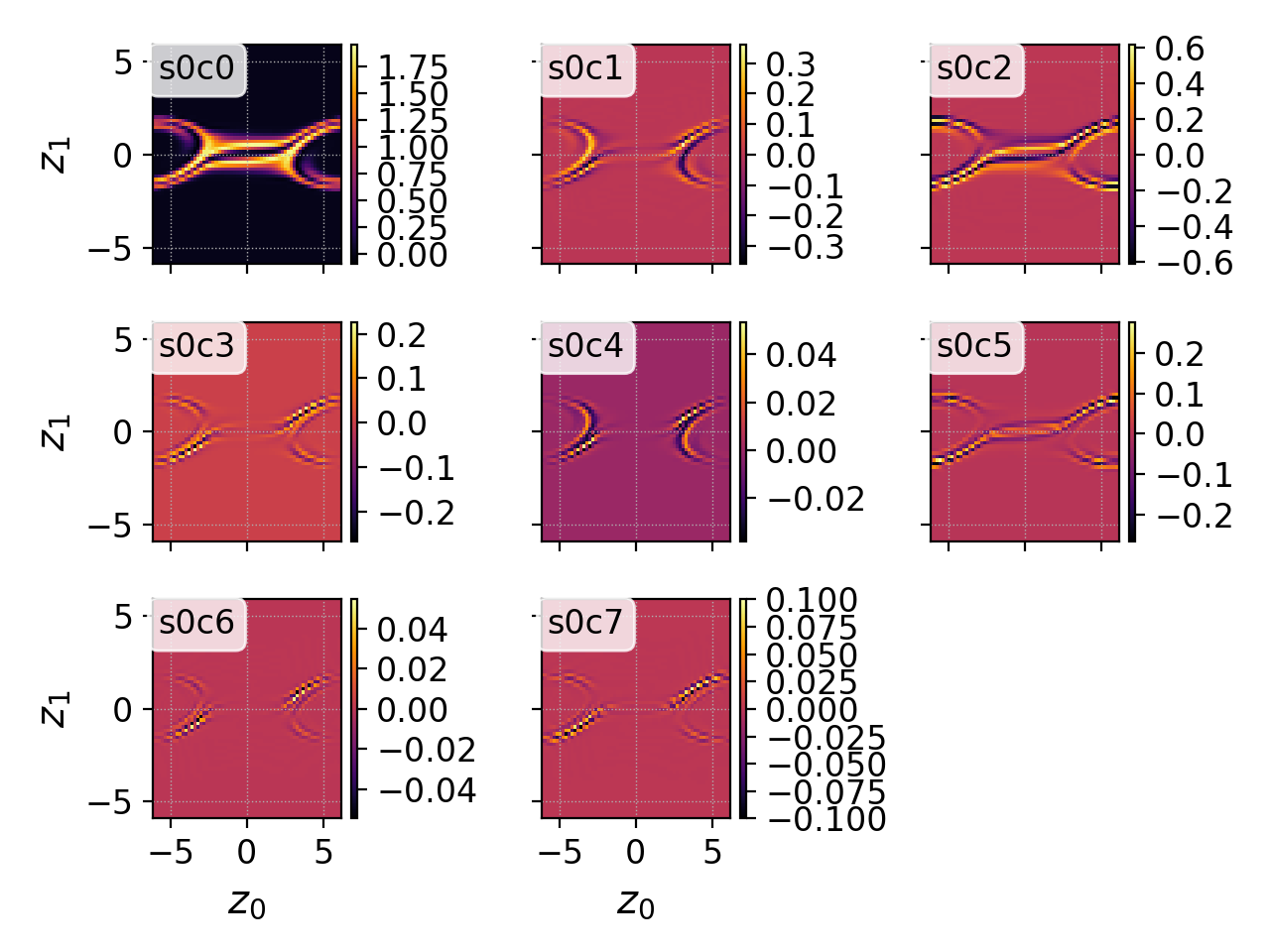
1 $ pgkyl -f two-stream64_elc_100.bp plot

By default, Postgkyl assumes that when plotting data with multiple components, user wants to compare them. Therefore, in this case, it outputs 2D plots for eight expansion coefficients for the basis from Eq. (2.56). Plotting just a single component can be achieved with the select command. Alternatively, Postgkyl can use the DG expansion coefficients to create uniform data with finer resolution using the interpolate command

⬇

1 $ pgkyl -f two-stream64_elc_100.bp interpolate -p2 -b ms plot

The result is in Fig. A.2. Note that the interpolate command is included before plot (more on that later) and has its own flags: -p for polynomial order and -b for basis.

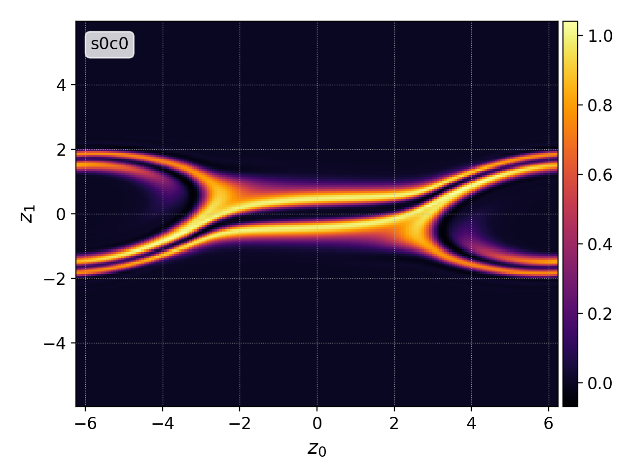
Note that the axis are by default labeled with neutral phase space coordinate $z_{i}$ . These labels are set at the beginning and are persistent through the Postgkyl command; therefore, if the initial data are 1X2V and the second component is integrated out for plotting (as it is the case for Weible instability in Sec. 4.3.3), Postgkyl will plot $z_{0}$ versus $z_{2}$ . Alternatively, labels can be manually set by plot flags

⬇

1 $ pgkyl -f two-stream64_elc_100.bp interpolate -p2 -b ms plot -x’$x$’ -y’$v_x$’

A.3 Terminal/Script Duality

Postgkyl is designed with the terminal/script duality in mind. This is important because even thought the majority of Postgkyl usage probably comes from terminal mode, it is common to carefully craft plotting scripts for publications³³ 3 For example, all the plotting scripts for this work are stored in Jupyter notebooks for each of the chapters. and these scripts are required to load data as well. Therefore, most of the Postgkyl functionality comes from Python functions, which are accessible from a Python script as well. The terminal commands are only click⁴⁴ 4 click is a useful Python package for handling command line inputs; http://click.pocoo.org/5/ wrappers for these functions. For example, data file loading

⬇

1 $ pgkyl -f two-stream64_elc_100.bp

can be exactly reproduced in a script with

⬇

1 import postgkyl as pg

2 data = pg.GData(’two-stream64_elc_100.bp’)

A.4 Chaining of Commands

The true strength of Postgkyl comes from the almost unlimited command chaining options, which is enabled by the click package mentioned above. In essence, the command chains are similar to Unix pipes, As data are pushed through series of commands, result of one command being feed to the next one. This feature has been already shown in this section, when the interpolate command was inserted before plot. This allows to build potentially complex diagnostics out of simple pieces, enhancing usefulness of each command.

For example, Postgkyl can be used to probe an evolution of the velocity profiles in the middle of the domain during the course of instability. A single lineout can be created with the select⁵⁵ 5 select is used to specify a coordinate and/or a component for lineout. For example, selecting component 1 and creating 1D data for $x=0$ (zeroth coordinate since Python is zero-index language)) is done with select --c0 0.0 --component 1. Note that when the coordinate flag is given integer instead of float-point number, lineout is done based on coordinate index rather than value. command. An example of this is in Fig. A.3.

Chaining of commands can become even more useful by loading multiple files at once with wild-card characters and then using the collect command, which stacks multiple data one after another, e.g., creates 2D data out of a set of 1D lineouts:

⬇

1 pgkyl -f ’two-stream64_elc_[0-9]*.bp’ interpolate -p2 -b ms select --c0 0.0 collect plot -x’$t$’ -y’$v_x$’

Note that for wild-card loading, the file name must be in quotes. The [0-9] wild-card stands for any single number; this is required to exclude diagnostic moment data like two-stream64_elc_M0_0.bp. The result of this command is in Fig. A.4, which provides quite a lot of insight into the instability. It captures the decrease of kinetic energy of the beams, as it is transformed into the electric field energy, and the nonlinear phase space mixing later in time.

With a simple change, Postgkyl can also integrate data along $x$ instead of selecting $x=0$ before stacking. As seen in Fig. A.5, this produces quite a different view.

With the same ease, Postgkyl can, for example, combine collect with fft to create spectrograms. There are no enforced limits for the chaining. This puts a responsibility on the user to make sure that the command chain is meaningful. For example, repeating the interpolate command results in an error because after the first command, data no longer have the valid form of DG expansion coefficients. As a final note, command chains can be made more compact and less readable by using only the shortest unique combination of starting letters for each command

⬇

1 pgkyl -f ’two-stream64_elc_[0-9]*.bp’ inter -p2 -b ms s --c0 0.0 c pl -x’$t$’ -y’$v_x$’

Appendix B Derivation of the Kinetic Weibel Instability Dispersion Relation

‘Obvious’ is the most dangerous word in mathematics.

E. T. Bell

This Appendix provides the comprehensive derivation of the kinetic Weibel instability dispersion relation Eq. (4.2).

B.1 Linearized Equations

Similar to the other instabilities, the derivation starts with the linearizion of the Vlasov equation (Eq. 2.11). However, the full Lorentz force (Eq. 2.4) must be taken into the account. Since $\bm{B}_{1}=(0,0,B_{z,1})$ and $\bm{k}=(k_{x},0,0)$ , we get

\displaystyle-i\omega f_{1}^{\pm}+iv_{x}k_{x}f_{1}^{\pm}+\frac{q}{m}\left[(E_{x,1}+v_{y}B_{z,1})\partial_{v_{x}}f_{0}^{\pm}+(E_{y,1}-v_{x}B_{z,1})\partial_{v_{y}}f_{0}^{\pm}\right]=0.

Then,¹¹ 1 Minus sign coming from moving $i$ to the numerator.

\displaystyle f_{1}^{\pm}=-\frac{iq}{m(\omega-v_{x}k_{x})}\left[(E_{x,1}+v_{y}B_{z,1})\partial_{v_{x}}f_{0}^{\pm}+(E_{y,1}-v_{x}B_{z,1})\partial_{v_{y}}f_{0}^{\pm}\right].

(B.1)

The Faraday’s law (Eq. 2.28),

\displaystyle i\begin{pmatrix}k_{y}E_{z,1}-k_{z}E_{y,1}\\ k_{z}E_{x,1}-k_{x}E_{z,1}\\ k_{x}E_{y,1}-k_{y}E_{x,1}\end{pmatrix}=i\omega\begin{pmatrix}B_{x,1}\\ B_{y,1}\\ B_{z,1}\end{pmatrix},

simplifies to

\displaystyle k_{x}E_{y,1}=\omega B_{z,1}.

(B.2)

Finally, as it is discussed in Sec. 4.2, linearizing the Ampere’s law (Eq. 2.29) gives

\displaystyle-ik_{x}B_{z,1}=\mu_{0}q\sum_{\pm}\left(\int v_{y}f_{1}^{\pm}\,d\bm{v}\right)-\frac{i\omega}{c^{2}}E_{y,1}.

(B.3)

B.2 Dispersion Relation

Substituting the perturbed distribution function (Eq. B.1) into Eq. (B.3) gives

\displaystyle-ik_{x}B_{z,1}=\mu_{0}\frac{-iq^{2}}{m}\sum_{\pm}\int v_{y}\frac{(E_{x,1}+v_{y}B_{z,1})\partial_{v_{x}}f_{0}^{\pm}+(E_{y,1}-v_{x}B_{z,1})\partial_{v_{y}}f_{0}^{\pm}}{\omega-v_{x}k_{x}}d\bm{v}-\frac{i\omega}{c^{2}}E_{y,1}.

The equation then can be simplified²² 2 Using $\omega_{pe}^{2}=nq^{2}/(\varepsilon_{0}m)$ and $c^{2}=1/(\varepsilon_{0}\mu_{0})$ . and slightly rearranged,

\displaystyle B_{z,1}=\frac{\omega_{pe}^{2}}{c^{2}k_{x}^{2}n}\sum_{\pm}\int\Big[\underbracket{\frac{v_{y}E_{x,1}\partial_{v_{x}}f_{0}^{\pm}}{\frac{\omega}{k_{x}}-v_{x}}}_{\text{I}}+\underbracket{\frac{v_{y}^{2}B_{z,1}\partial_{v_{x}}f_{0}^{\pm}}{\frac{\omega}{k_{x}}-v_{x}}}_{\text{II}}+\underbracket{\frac{v_{y}E_{y,1}\partial_{v_{y}}f_{0}^{\pm}}{\frac{\omega}{k_{x}}-v_{x}}}_{\text{III}}-\underbracket{\frac{v_{y}v_{x}B_{z,1}\partial_{v_{y}}f_{0}^{\pm}}{\frac{\omega}{k_{x}}-v_{x}}}_{\text{IV}}\Big]d\bm{v}+\frac{\omega}{c^{2}k_{x}}E_{y,1}.

(B.4)

Similar to Sec. 3.1.1, the distribution function can be factorized,

\displaystyle\int_{\mathcal{V}}f_{0}^{\pm}\,d\bm{v}=n\int_{-\infty}^{\infty}\int_{-\infty}^{\infty}f_{xy,0}^{\pm}\,dv_{x}dv_{y}\underbracket{\int_{-\infty}^{\infty}f_{z,0}\,dv_{z}}_{=1},

where $f_{xy,0}^{\pm}$ are assumed to be 2D Maxwellians,

\displaystyle f_{xy,0}^{\pm}=\frac{1}{2\pi v_{th}^{2}}\exp\left(-\frac{v_{x}^{2}+(v_{y}\pm u_{y})^{2}}{2v_{th}^{2}}\right).

The derivatives of the Maxwellians can be readily evaluated

	$\displaystyle\partial_{v_{x}}f_{xy,0}^{\pm}$	$\displaystyle=-\frac{v_{x}}{v_{th}^{2}}\frac{1}{2\pi v_{th}^{2}}\exp\left(-\frac{v_{x}^{2}+(v_{y}\pm u_{y})^{2}}{2v_{th}^{2}}\right),$		(B.5)
	$\displaystyle\partial_{v_{y}}f_{xy,0}^{\pm}$	$\displaystyle=-\frac{v_{y}\pm u_{y}}{v_{th}^{2}}\frac{1}{2\pi v_{th}^{2}}\exp\left(-\frac{v_{x}^{2}+(v_{y}\pm u_{y})^{2}}{2v_{th}^{2}}\right).$		(B.6)

The derivatives are then substituted into Eq. (B.4) and each term is assessed individually.

First Term

Splitting the integrals gives

\displaystyle\begin{aligned} \sum_{\pm}\int_{-\infty}^{\infty}\int_{-\infty}^{\infty}\frac{v_{y}E_{x,1}\partial_{v_{x}}f_{xy,0}^{\pm}}{\frac{\omega}{k_{x}}-v_{x}}\,dv_{x}dv_{y}=&-\sum_{\pm}\int_{-\infty}^{\infty}\int_{-\infty}^{\infty}\frac{v_{y}E_{x,1}\frac{v_{x}}{v_{th}^{2}}\frac{1}{2\pi v_{th}^{2}}\exp\left(-\frac{v_{x}^{2}+(v_{y}\pm u_{y})^{2}}{2v_{th}^{2}}\right)}{\frac{\omega}{k_{x}}-v_{x}}\,dv_{x}dv_{y},\\ =&-\frac{E_{x,1}}{\pi}\sum_{\pm}\int_{-\infty}^{\infty}\frac{\frac{v_{x}}{v_{th}^{2}}\exp\left(-\frac{v_{x}^{2}}{2v_{th}^{2}}\right)}{\frac{\omega}{k_{x}}-v_{x}}\,\frac{dv_{x}}{\sqrt{2v_{th}^{2}}}\times\\ &\int_{-\infty}^{\infty}v_{y}\exp\left(-\frac{(v_{y}\pm u_{y})^{2}}{2v_{th}^{2}}\right)\,\frac{dv_{y}}{\sqrt{2v_{th}^{2}}}.\end{aligned}

Now the $v_{y}$ before the exponential function in the second integral can be substituted with $v_{y}\pm u_{y}$ .³³ 3 The added terms cancel out because of the summation over the both populations, $\displaystyle\sum_{\pm}\int_{-\infty}^{\infty}(v_{y}\pm u_{y})\exp\left(-\frac{(v_{y}\pm u_{y})^{2}}{2v_{th}^{2}}\right)\,dv_{y}=$ $\displaystyle\sum_{\pm}\int_{-\infty}^{\infty}v_{y}\exp\left(-\frac{(v_{y}\pm u_{y})^{2}}{2v_{th}^{2}}\right)\,dv_{y}+$ $\displaystyle\underbracket{u_{y}\int_{-\infty}^{\infty}\exp\left(-\frac{(v_{y}+u_{y})^{2}}{2v_{th}^{2}}\right)\,dv_{y}-u_{y}\int_{-\infty}^{\infty}\exp\left(-\frac{(v_{y}-u_{y})^{2}}{2v_{th}^{2}}\right)\,dv_{y}}_{=0}.$ The integral is then calculated from an odd function of $v_{y}\pm u_{y}$ , which is defined for both $\pm\infty$ ,

\displaystyle\int_{-\infty}^{\infty}(v_{y}\pm u_{y})\exp\left(-\frac{(v_{y}\pm u_{y})^{2}}{2v_{th}^{2}}\right)\,d(v_{y}\pm u_{y})=0,

and, therefore, the entire first term is zero.

Second Term

Splitting the second term gives

\displaystyle\begin{aligned} \sum_{\pm}\int_{-\infty}^{\infty}\int_{-\infty}^{\infty}\frac{v_{y}^{2}B_{z,1}\partial_{v_{x}}f_{xy,0}^{\pm}}{\frac{\omega}{k_{x}}-v_{x}}\,dv_{x}dv_{y}=&-\sum_{\pm}\int_{-\infty}^{\infty}\int_{-\infty}^{\infty}\frac{v_{y}^{2}B_{z,1}\frac{v_{x}}{v_{th}^{2}}\frac{1}{2\pi v_{th}^{2}}\exp\left(-\frac{v_{x}^{2}+(v_{y}\pm u_{y})^{2}}{2v_{th}^{2}}\right)}{\frac{\omega}{k_{x}}-v_{x}}\,dv_{x}dv_{y},\\ =&-\frac{B_{z,1}}{\pi}\sum_{\pm}\int_{-\infty}^{\infty}\frac{\frac{v_{x}}{v_{th}^{2}}\exp\left(-\frac{v_{x}^{2}}{2v_{th}^{2}}\right)}{\frac{\omega}{k_{x}}-v_{x}}\frac{dv_{x}}{\sqrt{2v_{th}^{2}}}\times\\ &\int_{-\infty}^{\infty}v_{y}^{2}\exp\left(-\frac{(v_{y}\pm u_{y})^{2}}{2v_{th}^{2}}\right)\frac{dv_{y}}{\sqrt{2v_{th}^{2}}},\\ =&-\frac{B_{z,1}}{\pi}\sum_{\pm}\int_{-\infty}^{\infty}\frac{\sqrt{\frac{2}{v_{th}^{2}}}\frac{v_{x}}{\sqrt{2v_{th}^{2}}}\exp\left(-\frac{v_{x}^{2}}{2v_{th}^{2}}\right)}{\frac{\sqrt{2v_{th}^{2}}}{\sqrt{2v_{th}^{2}}}\left(\frac{\omega}{k_{x}}-v_{x}\right)}\frac{dv_{x}}{\sqrt{2v_{th}^{2}}}\times\\ &\int_{-\infty}^{\infty}v_{y}^{2}\exp\left(-\frac{(v_{y}\pm u_{y})^{2}}{2v_{th}^{2}}\right)\frac{dv_{y}}{\sqrt{2v_{th}^{2}}}.\end{aligned}

Now using the substitution,

\displaystyle\chi_{x}:=\frac{v_{x}}{\sqrt{2v_{th}^{2}}},\quad\zeta:=\frac{\omega/k_{x}}{\sqrt{2v_{th}^{2}}},\quad\chi_{y}^{\pm}:=\frac{v_{y}\pm u_{y}}{\sqrt{2v_{th}^{2}}}.

the equation simplifies to⁴⁴ 4 Note that this substitution leads to $d\chi_{x}=dv_{x}/\sqrt{2v_{th}^{2}}$ and $d\chi_{y}=dv_{y}/\sqrt{2v_{th}^{2}}$ .

	$\displaystyle\sum_{\pm}\int_{-\infty}^{\infty}\int_{-\infty}^{\infty}\frac{v_{y}^{2}B_{z,1}\partial_{v_{x}}f_{xy,0}^{\pm}}{\frac{\omega}{k_{x}}-v_{x}}\,dv_{x}dv_{y}$	$\displaystyle=-\frac{B_{z,1}}{\pi v_{th}^{2}}\sum_{\pm}\int_{-\infty}^{\infty}\frac{\chi_{x}\exp(-\chi_{x}^{2})}{\zeta-\chi_{x}}\,d\chi_{x}\int_{-\infty}^{\infty}v_{y}^{2}\exp(-(\chi_{y}^{\pm})^{2})\,d\chi_{y}^{\pm},$
		$\displaystyle=-\frac{B_{z,1}}{2\sqrt{\pi}v_{th}^{2}}\sum_{\pm}Z^{\prime}(\zeta)\int_{-\infty}^{\infty}v_{y}^{2}\exp(-(\chi_{y}^{\pm})^{2})\,d\chi_{y}^{\pm}.$

Finally, $v_{y}^{2}$ needs to be expressed in terms of $\chi_{y}^{2}$ in order to perform the integration,

	$\displaystyle v_{y}^{2}$	$\displaystyle=(v_{y}\pm u_{y})^{2}\mp 2v_{y}u_{y}-u_{y}^{2},$
		$\displaystyle=(v_{y}\pm u_{y})^{2}\mp 2(v_{y}\pm u_{y})u_{y}+2u_{y}^{2}-u_{y}^{2},$
		$\displaystyle=2v_{th}^{2}(\chi_{y}^{\pm})^{2}\mp 2\sqrt{(2v_{th}^{2})}\chi_{y}^{\pm}u_{y}+u_{y}^{2}.$

The middle term, $2\sqrt{(}2v_{th}^{2})\chi_{y}^{\pm}u_{y}$ , will have no effect on the result, because it integrates to zero as an odd function. Substituting the rest and using Gauss integrals⁵⁵ 5 $\int_{-\infty}^{\infty}\exp(-x^{2})=\sqrt{\pi}$ and $\int_{-\infty}^{\infty}x^{2}\exp(-x^{2})=\sqrt{\pi}/2$ . gives

\displaystyle\begin{aligned} \sum_{\pm}\int_{-\infty}^{\infty}\int_{-\infty}^{\infty}\frac{v_{y}^{2}B_{z,1}\partial_{v_{x}}f_{xy,0}^{\pm}}{\frac{\omega}{k_{x}}-v_{x}}\,dv_{x}dv_{y}&=-\frac{B_{z,1}}{2\sqrt{\pi}v_{th}^{2}}\sum_{\pm}Z^{\prime}(\zeta)\int_{-\infty}^{\infty}\left[(2v_{th}^{2}(\chi_{y}^{\pm})^{2}+u_{y}^{2}\right]\exp(-(\chi_{y}^{\pm})^{2})\,d\chi_{y}^{\pm},\\ &=-\sum_{\pm}\frac{B_{z,1}}{2}Z^{\prime}(\zeta)\left(\frac{u_{y}^{2}}{v_{th}^{2}}+1\right),\\ &=-B_{z,1}Z^{\prime}(\zeta)\left(\frac{u_{y}^{2}}{v_{th}^{2}}+1\right).\end{aligned}

Third Term

Splitting the third term gives

\displaystyle\begin{aligned} \sum_{\pm}\int_{-\infty}^{\infty}\int_{-\infty}^{\infty}\frac{v_{y}E_{y,1}\partial_{v_{y}}f_{xy,0}^{\pm}}{\frac{\omega}{k_{x}}-v_{x}}\,dv_{x}dv_{y}=&-\sum_{\pm}\int_{-\infty}^{\infty}\int_{-\infty}^{\infty}\frac{v_{y}E_{y,1}\frac{v_{y}\pm u_{y}}{v_{th}^{2}}\frac{1}{2\pi v_{th}^{2}}\exp\left(-\frac{v_{x}^{2}+(v_{y}\pm u_{y})^{2}}{2v_{th}^{2}}\right)}{\frac{\omega}{k_{x}}-v_{x}}\,dv_{x}dv_{y},\\ =&-\frac{E_{y,1}}{\pi}\sum_{\pm}\int_{-\infty}^{\infty}\frac{\exp\left(-\frac{v_{x}^{2}}{2v_{th}^{2}}\right)}{\frac{\omega}{k_{x}}-v_{x}}\frac{dv_{x}}{\sqrt{2v_{th}^{2}}}\times\\ &\int_{-\infty}^{\infty}v_{y}\frac{v_{y}\pm u_{y}}{v_{th}^{2}}\exp\left(-\frac{(v_{y}\pm u_{y})^{2}}{2v_{th}^{2}}\right)\frac{dv_{y}}{\sqrt{2v_{th}^{2}}}\end{aligned}

Similar to the first term, we substitute $v_{y}\pm u_{y}$ for $v_{y}$ in the second integral,

\displaystyle\begin{aligned} \sum_{\pm}\int_{-\infty}^{\infty}\int_{-\infty}^{\infty}\frac{v_{y}E_{y,1}\partial_{v_{y}}f_{xy,0}^{\pm}}{\frac{\omega}{k_{x}}-v_{x}}\,dv_{x}dv_{y}&=-\frac{E_{y,1}}{\pi}\sum_{\pm}\int_{-\infty}^{\infty}\frac{\exp\left(-\frac{v_{x}^{2}}{2v_{th}^{2}}\right)}{\frac{\omega}{k_{x}}-v_{x}}\frac{dv_{x}}{\sqrt{2v_{th}^{2}}}\times\\ &\int_{-\infty}^{\infty}2\frac{(v_{y}\pm u_{y})^{2}}{2v_{th}^{2}}\exp\left(-\frac{(v_{y}\pm u_{y})^{2}}{2v_{th}^{2}}\right)\frac{dv_{y}}{\sqrt{2v_{th}^{2}}},\\ =&-\frac{E_{y,1}}{\sqrt{2v_{th}^{2}}\pi}\sum_{\pm}\int_{-\infty}^{\infty}\frac{\exp(-\chi_{x}^{2})}{\zeta-\chi_{x}}\,d\chi_{x}\int_{-\infty}^{\infty}2(\chi_{y}^{\pm})^{2}\exp(-(\chi_{y}^{\pm})^{2})\,d\chi_{y}^{\pm},\\ =&\sum_{\pm}\frac{E_{y,1}}{\sqrt{2v_{th}^{2}}}Z(\zeta),\\ =&\frac{2E_{y,1}}{\sqrt{2v_{th}^{2}}}Z(\zeta).\end{aligned}

Fourth Term

Finally, splitting the fourth term

\displaystyle\begin{aligned} \sum_{\pm}\int_{-\infty}^{\infty}\int_{-\infty}^{\infty}\frac{-v_{y}v_{x}B_{z,1}\partial_{v_{y}}f_{xy,0}^{\pm}}{\frac{\omega}{k_{x}}-v_{x}}\,dv_{x}dv_{y}=&\sum_{\pm}\int_{-\infty}^{\infty}\int_{-\infty}^{\infty}\frac{v_{y}v_{x}B_{z,1}\frac{v_{y}\pm u_{y}}{v_{th}^{2}}\frac{1}{2\pi v_{th}^{2}}\exp\left(-\frac{v_{x}^{2}+(v_{y}\pm u_{y})^{2}}{2v_{th}^{2}}\right)}{\frac{\omega}{k_{x}}-v_{x}}\,dv_{x}dv_{y},\\ =&\frac{B_{z,1}}{\pi}\sum_{\pm}\int_{-\infty}^{\infty}\frac{v_{x}\exp\left(-\frac{v_{x}^{2}}{2v_{th}^{2}}\right)}{\frac{\omega}{k_{x}}-v_{x}}\frac{dv_{x}}{\sqrt{2v_{th}^{2}}}\times\\ &\int_{-\infty}^{\infty}v_{y}\frac{v_{y}\pm u_{y}}{v_{th}^{2}}\exp\left(-\frac{(v_{y}\pm u_{y})^{2}}{2v_{th}^{2}}\right)\frac{dv_{y}}{\sqrt{2v_{th}^{2}}},\\ =&\frac{B_{z,1}}{\pi}\sum_{\pm}\int_{-\infty}^{\infty}\frac{v_{x}\exp\left(-\frac{v_{x}^{2}}{2v_{th}^{2}}\right)}{\frac{\omega}{k_{x}}-v_{x}}\frac{dv_{x}}{\sqrt{2v_{th}^{2}}}\times\\ &\int_{-\infty}^{\infty}2\frac{(v_{y}\pm u_{y})^{2}}{2v_{th}^{2}}\exp\left(-\frac{(v_{y}\pm u_{y})^{2}}{2v_{th}^{2}}\right)\frac{dv_{y}}{\sqrt{2v_{th}^{2}}},\\ =&\frac{B_{z,1}}{\pi}\sum_{\pm}\int_{-\infty}^{\infty}\frac{\chi_{x}\exp(-\chi_{x}^{2})}{\zeta-\chi_{x}}\,d\chi_{x}\int_{-\infty}^{\infty}2\chi_{y}^{\pm}\exp(-(\chi_{y}^{\pm})^{2})\,d\chi_{y}^{\pm},\\ =&\sum_{\pm}\frac{B_{z,1}}{2}Z^{\prime}(\zeta).\\ =&B_{z,1}Z^{\prime}(\zeta).\end{aligned}

Combining the Terms

Putting everything together gives

\displaystyle B_{z,1}=\frac{\omega_{pe}^{2}}{c^{2}k_{x}^{2}}\left[-B_{z,1}Z^{\prime}(\zeta)\left(\frac{u_{y}^{2}}{v_{th}^{2}}+1\right)+\frac{2E_{y,1}}{\sqrt{2v_{th}^{2}}}Z(\zeta)+B_{z,1}Z^{\prime}(\zeta)\right]+\frac{\omega}{c^{2}k_{x}}E_{y,1}.

As a final step, $E_{y,1}$ is substituted for from Faraday’s law (Eq. B.2),

\displaystyle\begin{aligned} B_{z,1}&=\frac{\omega_{pe}^{2}}{c^{2}k_{x}^{2}}\left[-B_{z,1}Z^{\prime}(\zeta)\frac{u_{y}^{2}}{v_{th}^{2}}+2\frac{\omega B_{z,1}}{\sqrt{2v_{th}^{2}}k_{x}}Z(\zeta)\right]+\frac{\omega^{2}}{c^{2}k_{x}^{2}}B_{z,1},\\ 1&=\frac{\omega_{pe}^{2}}{c^{2}k_{x}^{2}}\left[-Z^{\prime}(\zeta)\frac{u_{d}^{2}}{v_{th}^{2}}+2\zeta Z(\zeta)\right]+\frac{\omega^{2}}{c^{2}k_{x}^{2}},\end{aligned}

which is a single equation with one unknown $\omega$ . Eq. (3.9) can be used for the final rearrangement to obtain Eq. (4.2),

\displaystyle\frac{1}{2}=\frac{\omega_{pe}^{2}}{c^{2}k_{x}^{2}}\left[\zeta Z(\zeta)\left(1+\frac{u_{y}^{2}}{v_{th}^{2}}\right)+\frac{u_{y}^{2}}{v_{th}^{2}}\right]+\frac{v_{th}^{2}}{c^{2}}\zeta^{2}

Appendix C Gkeyll Input Files

This appendix provides a list of the Gkeyll 2.0 input files for the simulations mentioned in the text. For testing purposes, Gkeyll executable is readily available through Anaconda package manager conda and can be installed with just a single command:

⬇

1 conda install -c gkyl gkyl

C.1 Reflection of the Neutral Gas

⬇

1 -- Gkyl --------------------------------------------------------------

2 -- Neutral gass bouncing between two walls ---------------------------

3 local Plasma = require "App.PlasmaOnCartGrid"

5 vth = 0.1

6 vd = 1.0

8 -- initialization function

9 local function maxwellian(n, vd, vth, v)

10 return n / math.sqrt(2*math.pi*vth*vth) *

11 math.exp(-(v-vd)^2/(2*vth*vth))

12 end

14 sim = Plasma.App {

15 logToFile = false,

17 tEnd = 20, -- end time

18 nFrame = 5, -- number of output frames

19 lower = {-5.0}, -- configuration space lower left

20 upper = {5.0}, -- configuration space upper right

21 cells = {128}, -- configuration space cells

22 basis = "serendipity", -- one of "serendipity" or "maximal-order"

23 polyOrder = 2, -- polynomial order

24 cflFrac = 1.0, -- CFL "fraction". Usually 1.0

25 timeStepper = "rk3", -- one of "rk2" or "rk3"

27 -- decomposition for configuration space

28 decompCuts = {2}, -- cuts in each configuration direction

29 useShared = false, -- if to use shared memory

31 -- boundary conditions for configuration space

32 periodicDirs = {}, -- periodic directions

34 -- electrons

35 neut = Plasma.VlasovSpecies {

36 charge = 0.0, mass = 1.0,

37 -- velocity space grid

38 lower = {-2.0},

39 upper = {2.0},

40 cells = {48},

41 decompCuts = {1},

42 -- initial conditions

43 init = function (t, xn)

44 local x, v = xn[1], xn[2]

45 return maxwellian(1.0, vd, vth, v)*math.exp(-x^2)

46 end,

47 evolve = true, -- evolve species?

48 bcx = { Plasma.VlasovSpecies.bcReflect,

49 Plasma.VlasovSpecies.bcReflect },

50 diagnosticMoments = { "M0", "M1i", "M2" },

51 },

52 }

53 -- run application

54 sim:run()

C.2 Landau Damping of Langmuir Wave

⬇

1 -- Gkyl --------------------------------------------------------------

2 -- Landau damping of Langmuir waves ----------------------------------

3 local Plasma = require "App.PlasmaOnCartGrid"

5 -- Parameters

6 local epsilon_0, mu_0 = 1.0, 1.0

7 local elemCharge = 1.0

8 local q_e, q_i = -elemCharge, elemCharge

9 local m_e, m_i = 1.0, 1836.0

10 local n_e, n_i = 1.0, 1.0

11 local T_e, T_i = 1.0, 1.0

12 local vth_e, vth_i = math.sqrt(T_e/m_e), math.sqrt(T_i/m_i)

13 local vd_e, vd_i = 0.0, 0.0

15 local omega_pe = math.sqrt((n_e * q_e^2)/(epsilon_0*m_e))

16 local lambda_D = math.sqrt((epsilon_0 * T_e)/(n_e * q_e^2))

17 -- artificially decrease the speed of light

18 local c = 10*vth_e

19 mu_0 = 1.0/(epsilon_0 * c^2)

21 -- Perturbations

22 kNumber = 0.5/lambda_D

23 A = 1e-1

25 -- initialization function

26 local function maxwellian1D(n, vd, vth, vx)

27 return n / math.sqrt(2*math.pi*vth*vth) *

28 math.exp(-(vx-vd)^2/(2*vth*vth))

29 end

31 local tEnd = 20/omega_pe

33 sim = Plasma.App {

34 logToFile = false,

36 tEnd = tEnd, -- end time

37 nFrame = 100, -- number of output frames

38 lower = {0.0}, -- configuration space lower left

39 upper = {2*math.pi/kNumber}, -- configuration space upper right

40 cells = {64}, -- configuration space cells

41 basis = "serendipity", -- one of "serendipity" or "maximal-order"

42 polyOrder = 2, -- polynomial order

43 cflFrac = 1.0, -- CFL "fraction". Usually 1.0

44 timeStepper = "rk3", -- one of "rk2" or "rk3"

46 -- decomposition for configuration space

47 decompCuts = {2}, -- cuts in each configuration direction

48 useShared = false, -- if to use shared memory

49 -- boundary conditions for configuration space

50 periodicDirs = {1},

52 -- electrons

53 elc = Plasma.VlasovSpecies {

54 charge = q_e, mass = m_e,

55 -- velocity space grid

56 lower = {-6.0*vth_e},

57 upper = {6.0*vth_e},

58 cells = {128},

59 decompCuts = {1},

60 -- initial conditions

61 init = function (t, xn)

62 local x, vx = xn[1], xn[2]

63 return maxwellian1D(n_e, vd_e, vth_e, vx) *

64 (1 + A * math.cos(kNumber*x))

65 end,

66 evolve = true,

67 diagnosticMoments = { "M0", "M1i", "M2ij" },

68 },

70 ion = Plasma.VlasovSpecies {

71 charge = q_i, mass = m_i,

72 -- velocity space grid

73 lower = {-6.0*vth_i},

74 upper = {6.0*vth_i},

75 cells = {128},

76 decompCuts = {1},

77 -- initial conditions

78 init = function (t, xn)

79 local x, vx = xn[1], xn[2]

80 return maxwellian1D(n_i, vd_i, vth_i, vx)

81 end,

82 evolve = false, -- evolve species?

83 diagnosticMoments = { "M0", "M1i", "M2ij" },

84 },

86 -- field solver

87 field = Plasma.MaxwellField {

88 epsilon0 = epsilon_0, mu0 = mu_0,

89 init = function (t, xn)

90 local x = xn[1]

91 local E = A*q_e*n_e/kNumber/epsilon_0 * math.sin(kNumber*x)

92 return E, 0.0, 0.0, 0.0, 0.0, 0.0

93 end,

94 evolve = true, -- evolve field?

95 },

96 }

97 -- run application

98 sim:run()

C.3 Electron Two-stream Instability

⬇

1 -- Gkyl --------------------------------------------------------------

2 -- Electron Two-stream instability -----------------------------------

3 local Plasma = require "App.PlasmaOnCartGrid"

5 kNumber = 0.5 -- wave-number

6 vth_e = 0.2 -- electron thermal velocity

7 vd_e = 1.0 -- drift velocity

8 perturbation = 1.0e-6 -- distribution function perturbation

10 -- initialization function

11 local function maxwellian1D(n, vd, vth, vx)

12 return n / math.sqrt(2*math.pi*vth*vth) *

13 math.exp(-(vx-vd)^2/(2*vth*vth))

14 end

16 sim = Plasma.App {

17 logToFile = false,

19 tEnd = 50.0, -- end time

20 nFrame = 100, -- number of output frames

21 lower = {-math.pi/kNumber}, -- configuration space lower left

22 upper = {math.pi/kNumber}, -- configuration space upper right

23 cells = {64}, -- configuration space cells

24 basis = "serendipity", -- one of "serendipity" or "maximal-order"

25 polyOrder = 2, -- polynomial order

26 timeStepper = "rk3", -- one of "rk2", "rk3" or "rk3s4"

28 -- decomposition for configuration space

29 decompCuts = {8}, -- cuts in each configuration direction

30 useShared = false, -- if to use shared memory

31 -- boundary conditions for configuration space

32 periodicDirs = {1}, -- periodic directions

34 -- electrons

35 elc = Plasma.VlasovSpecies {

36 charge = -1.0, mass = 1.0,

37 -- velocity space grid

38 lower = {-6},

39 upper = {6},

40 cells = {32},

41 decompCuts = {1},

42 -- initial conditions

43 init = function (t, xn)

44 local x, v = xn[1], xn[2]

45 local f = maxwellian1D(0.5, vd_e, vth_e, v) + maxwellian1D(0.5, -vd_e, vth_e, v)

46 return (1 + perturbation*math.cos(kNumber*x)) * f

47 end,

48 evolve = true, -- evolve species?

50 diagnosticMoments = { "M0", "M1i", "M2" }

51 },

53 -- field solver

54 field = Plasma.MaxwellField {

55 epsilon0 = 1.0, mu0 = 1.0,

56 init = function (t, xn)

57 local x = xn[1]

58 local Ex = -perturbation * math.sin(kNumber*x) / kNumber

59 return Ex, 0.0, 0.0, 0.0, 0.0, 0.0

60 end,

61 evolve = true, -- evolve field?

62 },

63 }

64 -- run application

65 sim:run()

C.4 Weibel Instability

⬇

1 -- Gkyl --------------------------------------------------------------

2 -- Electron Weibel instability ---------------------------------------

3 local Plasma = require "App.PlasmaOnCartGrid"

5 -- Constants

6 q_e, m_e = -1.0, 1.0

7 epsilon_0, mu_0 = 1.0, 1.0

9 -- Initial conditions (’p’ for plus population and ’m’ for minus population)

10 n_ep, n_em = 0.5, 0.5

11 ux_ep, ux_em = 0.0, 0.0

12 uy_ep, uy_em = 0.15, -0.15

13 vth_ep, vth_em = 0.03, 0.03

14 -- T_ep, T_em = 0.01, 0.01

15 -- vth_ep, vth_em = math.sqrt(T_ep/m_e), math.sqrt(T_ep/m_e)

17 kx = 0.4-- wave-number

18 perturb = 1.0e-4 -- distribution function perturbation

20 -- Maxwellian in 1x2v

21 local function maxwellian2D(vx, vy, n, ux, uy, vth)

22 local v2 = (vx - ux)^2 + (vy - uy)^2

23 return n/(2*math.pi*vth^2)*math.exp(-v2/(2*vth^2))

24 end

26 sim = Plasma.App {

27 logToFile = false,

29 tEnd = 500.0, -- end time

30 nFrame = 500, -- number of output frames

31 lower = { 0.0 }, -- configuration space lower left

32 upper = { 2*math.pi/kx }, -- configuration space upper right

33 cells = {64}, -- configuration space cells

34 basis = "serendipity", -- one of "serendipity" or "maximal-order"

35 polyOrder = 2, -- polynomial order

36 timeStepper = "rk3", -- one of "rk2" or "rk3"

38 -- decomposition for configuration space

39 decompCuts = {2}, -- cuts in each configuration direction

40 useShared = false, -- if to use shared memory

41 -- boundary conditions for configuration space

42 periodicDirs = {1}, -- periodic directions

44 -- electrons

45 elc = Plasma.VlasovSpecies {

46 charge = q_e, mass = m_e,

47 -- velocity space grid

48 lower = {-1.0, -1.0},

49 upper = {1.0, 1.0},

50 cells = {32, 32},

51 decompCuts = {1, 1},

52 -- initial conditions

53 init = function (t, xn)

54 local x, vx, vy = xn[1], xn[2], xn[3]

55 return maxwellian2D(vx, vy, n_ep, ux_ep, uy_ep, vth_ep) +

56 maxwellian2D(vx, vy, n_em, ux_em, uy_em, vth_em)

57 end,

58 evolve = true, -- evolve species?

59 diagnosticMoments = { "M0", "M1i", "M2" }

60 },

62 -- field solver

63 field = Plasma.MaxwellField {

64 epsilon0 = epsilon_0, mu0 = mu_0,

65 init = function (t, xn)

66 local x = xn[1]

67 local Bz = perturb*math.sin(kx*x)

68 return 0.0, 0.0, 0.0, 0.0, 0.0, Bz

69 end,

70 evolve = true, -- evolve field?

71 },

72 }

73 -- run application

74 sim:run()

C.5 Collisionless Sheath

⬇

1 -- Gkyl --------------------------------------------------------------

2 -- Basic sheath simulation -------------------------------------------

3 local Plasma = require "App.PlasmaOnCartGrid"

5 -- SI units

6 local epsilon_0, mu_0 = 8.854e-12, 1.257e-6

7 local q_e, q_i = -1.6021766e-19, 1.6021766e-19

8 local m_e, m_i = 9.109383e-31, 1.6726218e-27

9 local n_e, n_i = 1.0e17, 1.0e17

10 local u_e, u_i = 0.0, 0.0

11 local T_e, T_i = 10*1.6021766e-19, 1*1.6021766e-19

13 local vth_e, vth_i = math.sqrt(T_e/m_e), math.sqrt(T_i/m_i)

14 local uB = math.sqrt(T_e/m_i)

15 -- artificially decrease the speed of light

16 mu_0 = 1.0/(epsilon_0 * (10*vth_e)^2)

17 --epsilon_0 = 1.0/(mu_0 * (10*vth_e)^2)

19 local omega_pe = math.sqrt((n_e * q_e^2)/(epsilon_0*m_e))

20 local lambda_D = math.sqrt((epsilon_0 * T_e)/(n_e * q_e^2))

22 -- initialization function

23 local function maxwellian(n, u, vth, v)

24 return n / math.sqrt(2*math.pi*vth*vth) *

25 math.exp(-(v-u)^2/(2*vth*vth))

26 end

28 sim = Plasma.App {

29 logToFile = false,

31 tEnd = 1000/omega_pe, -- end time

32 nFrame = 100, -- number of output frames

33 lower = {-128.0*lambda_D}, -- configuration space lower left

34 upper = {128.0*lambda_D}, -- configuration space upper right

35 cells = {256}, -- configuration space cells

36 basis = "serendipity", -- one of "serendipity" or "maximal-order"

37 polyOrder = 2, -- polynomial order

38 cflFrac = 1.0, -- CFL "fraction". Usually 1.0

39 timeStepper = "rk3", -- one of "rk2" or "rk3"

41 -- decomposition for configuration space

42 decompCuts = {8}, -- cuts in each configuration direction

43 useShared = false, -- if to use shared memory

45 -- boundary conditions for configuration space

46 periodicDirs = {}, -- periodic directions

48 -- electrons

49 elc = Plasma.VlasovSpecies {

50 charge = q_e, mass = m_e,

51 -- velocity space grid

52 lower = {-6.0*vth_e},

53 upper = {6.0*vth_e},

54 cells = {32},

55 decompCuts = {1},

56 -- initial conditions

57 init = function (t, xn)

58 local x, v = xn[1], xn[2]

59 return maxwellian(n_e, u_e, vth_e, v)

60 end,

61 evolve = true, -- evolve species?

62 bcx = { Plasma.VlasovSpecies.bcAbsorb,

63 Plasma.VlasovSpecies.bcAbsorb },

64 diagnosticMoments = { "M0", "M1i", "M2" },

65 },

67 ion = Plasma.VlasovSpecies {

68 charge = q_i, mass = m_i,

69 -- velocity space grid

70 lower = {-6.0*uB},

71 upper = {6.0*uB},

72 cells = {32},

73 decompCuts = {1},

74 -- initial conditions

75 init = function (t, xn)

76 local x, v = xn[1], xn[2]

77 return maxwellian(n_i, u_i, vth_i, v)

78 end,

79 evolve = true, -- evolve species?

80 bcx = { Plasma.VlasovSpecies.bcAbsorb,

81 Plasma.VlasovSpecies.bcAbsorb },

82 diagnosticMoments = { "M0", "M1i", "M2" },

83 },

85 -- field solver

86 field = Plasma.MaxwellField {

87 epsilon0 = epsilon_0, mu0 = mu_0,

88 init = function (t, xn)

89 return 0.0, 0.0, 0.0, 0.0, 0.0, 0.0

90 end,

91 evolve = true, -- evolve field?

92 bcx = { Plasma.MaxwellField.bcReflect,

93 Plasma.MaxwellField.bcReflect },

94 },

95 }

96 -- run application

97 sim:run()

C.6 Sod [1978] Shock Tube

⬇

1 -- Gkyl --------------------------------------------------------------

2 -- BGK Sod Shock Tube Test -------------------------------------------

3 local Plasma = require "App.PlasmaOnCartGrid"

5 -- left/right state for shock

6 local nl, ul, pl = 1.0, 0.0, 1.0

7 local nr, ur, pr = 0.125, 0.0, 0.1

9 local vthl = math.sqrt(pl/nl)

10 local vthr = math.sqrt(pr/nr)

12 local Kn = 0.001

14 local function maxwellian(n, u, vth, v)

15 return n / math.sqrt(2*math.pi*vth^2) *

16 math.exp(-(v-u)^2 / (2*vth^2))

17 end

19 sim = Plasma.App {

20 logToFile = false,

22 tEnd = 0.3, -- end time

23 nFrame = 8, -- number of frames to write

24 lower = {0.0}, -- configuration space lower left

25 upper = {1.0}, -- configuration space upper right

26 cells = {128}, -- configuration space cells

27 basis = "serendipity", -- one of "serendipity" or "maximal-order"

28 polyOrder = 2, -- polynomial order

29 timeStepper = "rk3", -- one of "rk2", "rk3" or "rk3s4"

31 -- decomposition for configuration space

32 decompCuts = {1}, -- cuts in each configuration direction

33 useShared = false, -- if to use shared memory

35 -- boundary conditions for configuration space

36 periodicDirs = {}, -- periodic directions

38 -- electrons

39 neut = Plasma.VlasovSpecies {

40 --nDiagnosticFrame = 2,

41 charge = 0.0, mass = 1.0,

42 -- velocity space grid

43 lower = {-6.0},

44 upper = {6.0},

45 cells = {32},

46 decompCuts = {1},

47 -- initial conditions

48 init = function (t, xn)

49 local x, v = xn[1], xn[2]

51 if math.abs(x) < 0.5 then

52 return maxwellian(nl, ul, vthl, v)

53 else

54 return maxwellian(nr, ur, vthr, v)

55 end

56 end,

57 bcx = { Plasma.VlasovSpecies.bcCopy,

58 Plasma.VlasovSpecies.bcCopy },

59 -- evolve species?

60 evolve = true,

61 -- diagnostic moments

62 diagnosticMoments = { "M0", "M1i", "M2" },

64 -- collisions

65 coll = Plasma.BgkCollisions {

66 collFreq = vthl/Kn,

67 },

68 },

69 }

70 -- run application

71 sim:run()

Appendix D Scripts and Algorithms

This appendix provides listings of miscellaneous scripts and algorithms used through this work.

D.1 Field Particle Correlation (Python)

⬇

1 import numpy as np

2 import matplotlib.pyplot as plt

3 import matplotlib.cm as cm

4 import postgkyl as pg

6 xIdx = 48

7 vIdx1 = 280

8 vIdx2 = 224

9 numFrame = 101

10 numV = 384

11 E = np.zeros(numFrame)

12 f = np.zeros((numFrame, numV))

13 C0 = np.zeros((numFrame, numV))

14 t = np.linspace(0., 20., numFrame)

15 v = np.linspace(-6., 6., numV)

16 q = -1.0

17 dt = 20/(numFrame-1)

19 for fIdx in range(numFrame):

20 data = pg.GData(’landau_field_{:d}.bp’.format(fIdx))

21 dg = pg.GInterpModal(data, 2, ’ms’)

22 grid, tmp = dg.interpolate(0)

23 E[fIdx] = tmp[xIdx, 0]

25 data = pg.GData(’landau_elc_{:d}.bp’.format(fIdx))

26 dg = pg.GInterpModal(data, 2, ’ms’)

27 grid, tmp = dg.differentiate(1)

28 df[fIdx, :] = tmp[xIdx, :, 0]

30 for vIdx in range(numV):

31 C0[:, vIdx] = -q * v[vIdx]**2 / 2 * (df[:, vIdx] - df[0, vIdx]) * E

33 fig, ax = plt.subplots(2, 2, sharex=True, sharey="row", figsize=(10,8))

35 minN = 10

36 maxN = 70

37 for N in range(minN, maxN):

38 tmp00 = np.full(numFrame, np.nan)

39 tmp01 = np.full(numFrame, np.nan)

40 tmp10 = np.zeros(numFrame)

41 tmp11 = np.zeros(numFrame)

42 for i in range(numFrame - N):

43 tmp00[i] = np.sum(C0[i : i+N, vIdx1]) / (N*dt)

44 tmp01[i] = np.sum(C0[i : i+N, vIdx2]) / (N*dt)

45 for i in range(1, numFrame):

46 tmp10[i] = np.sum(tmp00[:i])

47 tmp11[i] = np.sum(tmp01[:i])

48 ax[0, 0].plot(t, tmp00, color=cm.inferno((N-minN)/float(maxN-minN)))

49 ax[0, 1].plot(t, tmp01, color=cm.inferno((N-minN)/float(maxN-minN)))

50 tmp10 = tmp10 * dt

51 tmp11 = tmp11 * dt

52 ax[1, 0].plot(t, tmp10, color=cm.inferno((N-minN)/float(maxN-minN)))

53 ax[1, 1].plot(t, tmp11, color=cm.inferno((N-minN)/float(maxN-minN)))

D.2 Precomputation of Material-Based Boundary Condition File (Mathematica)

⬇

1 basis[x_, vx_] := {1/2, (Sqrt[3] x)/2, (Sqrt[3] vx)/2, (3 vx x)/2, (

2 3 Sqrt[5] (x^2 - 1/3))/4, (3 Sqrt[5] (vx^2 - 1/3))/4, (

3 3 Sqrt[15] (vx x^2 - vx/3))/4, (3 Sqrt[15] (vx^2 x - x/3))/4}

4 numBasis = 8;

5 \[Chi] = 1.0;

6 mc = 0.4;

7 \[Eta][E_, \[Xi]_] := Sqrt[1 - (E - \[Chi])/(mc E) (1 - \[Xi]^2)]

8 \[Xi]c[E_] :=

9 If[E < \[Chi]/(1 - mc), 0.0, Sqrt[1 - (mc E)/(E - \[Chi])]]

10 T[E_, \[Xi]_] := (

11 4 mc Sqrt[E - \[Chi]] \[Xi] Sqrt[

12 mc E] \[Eta][E, \[Xi]])/(mc Sqrt[E - \[Chi]] \[Xi] +

13 Sqrt[mc E] \[Eta][E, \[Xi]])^2

14 R[E_, \[Xi]_, C_] :=

15 If[E < \[Chi], 1.,

16 If[\[Xi] > \[Xi]c[E],

17 1. - T[E, \[Xi]]/(

18 1 + C/\[Xi]) - (C/\[Xi])/(1 + C/\[Xi])

19 NIntegrate[T[E, t], {t, \[Xi]c[E], 1.0}],

20 1. - (C/\[Xi])/(1 + C/\[Xi])

21 NIntegrate[T[E, t], {t, \[Xi]c[E], 1.0}]]]

22 elemCharge = 1.6021766*^-19;

23 me = 9.109383*^-31;

24 roughness = 2.0;

25 vth = Sqrt[(10*elemCharge)/me];

26 Nv = 32;

27 dv = Sqrt[(2*\[Chi]*elemCharge)/me]

28 vc = Table[(-(Nv/2) + 1/2 + i)*dv, {i, 0, Nv - 1}]

29 getE[vx_, vc_, dv_] := 1/2 me (vc + vx dv/2)^2/elemCharge;

30 fh = OpenWrite[NotebookDirectory[] <> "wall_1X1V.lua"];

31 WriteLine[fh, "local _M = {}"];

32 WriteLine[fh, "_M[1] = function (idx, f, out)"];

33 For[j = 1, j <= Nv, j++,

34 If[j == 1,

35 WriteLine[fh, " if idx[1] == " <> ToString[j] <> " then"],

36 WriteLine[fh, " elseif idx[1] == " <> ToString[j] <> " then"]];

37 For[k = 1, k <= numBasis, k++,

38 str = "";

39 For[l = 1, l <= numBasis, l++,

40 temp =

41 NIntegrate[

42 R[getE[vx, vc[[j]], dv], 1.0, roughness] * basis[-x, -vx][[l]]*

43 basis[x, vx][[k]], {x, -1, 1}, {vx, -1, 1}, MaxPoints -> 9];

44 If[temp != 0.0,

45 str = str <> " + " <> TextString[temp] <> "*f[" <> TextString[l] <>

46 "]"];

47 ];

48 WriteLine[fh, " out[" <> TextString[k] <> "] = 0.0" <> str];

49 ]

50 ]

51 WriteLine[fh, " end"];

52 WriteLine[fh, "end"];

53 WriteLine[fh, "return _M"];

54 Close[fh];