跳到论文正文
W Papers独立论文阅读器 arXiv:1809.06153 论文正文 计算阅读时间 · 0%
引用这篇论文根据当前论文元数据生成,正式投稿前建议核对。


License: arXiv.org perpetual non-exclusive license
arXiv:1809.06153v1 [math.PR] 17 Sep 2018

Long-time trajectorial large deviations for affine stochastic volatility models and application to variance reduction for option pricing

Zorana Grbac11 1 Université Paris Diderot, Paris, France

David Krief 1

Peter Tankov 122 2 ENSAE, Palaiseau, France

Abstract: This work extends the variance reduction method for the pricing of possibly path-dependent derivatives, which was developed in [Genin and Tankov, 2016] for exponential Lévy models, to affine stochastic volatility models [Keller-Ressel, 2011]. We begin by proving a pathwise large deviations principle for affine stochastic volatility models. We then apply a time-dependent Esscher transform to the affine process and use Varadhan’s Lemma, in the fashion of [Guasoni and Robertson, 2008] and [Robertson, 2010], to approximate the problem of finding the Esscher measure that minimises the variance of the Monte-Carlo estimator. We test the method on the Heston model with and without jumps to demonstrate the numerical efficiency of the method.

1. Introduction

The aim of this paper is to develop efficient importance sampling estimators for prices of path-dependent options in affine stochastic volatility (ASV) models of asset prices. To this end, we establish pathwise large deviation results for these models, which are of independent interest.

An ASV model, studied in [Keller-Ressel, 2011] is a two-dimensional affine process (X,V)(X,V) on ℝ×ℝ+\mathbb{R}\times\mathbb{R}_{+} with special properties, where XX models the logarithm of the stock price and VV its instantaneous variance. This class includes many well studied and widely used models such as Heston stochastic volatility model [Heston, 1993], the model of Bates [Bates, 1996], Barndorff-Nielsen stochastic volatility model [Barndorff-Nielsen and Shephard, 2001] and time-changed Lévy models with independent affine time change. European options in affine stochastic volatility models may be priced by Fourier transform, but for path-dependent options explicit formulas are in general not available and Monte Carlo is often the method of choice. At the same time, Monte Carlo simulation of such processes is difficult and time-consuming: the convergence rates of discretization schemes are often low due to the irregular nature of coefficients of the corresponding stochastic differential equations. To accelerate Monte Carlo simulation, it is thus important to develop efficient variance-reduction algorithms for these models.

In this paper, we therefore develop an importance sampling algorithm for ASV models. The importance sampling method is based on the following identity, valid for any probability measure ℚ\mathbb{Q}, with respect to which ℙ\mathbb{P} is absolutely continuous. Let PP be a deterministic function of a random trajectory SS, then

𝔼⁡[P⁡(S)]=𝔼ℚ​[d​ℙd​ℚ​P​(S)].\mathbb{E}[P(S)]=\mathbb{E}^{\mathbb{Q}}\left[\frac{d\mathbb{P}}{d\mathbb{Q}}P(S)\right].

This allows one to define the importance sampling estimator

P^Nℚ:=1N​∑j=1N[d​ℙd​ℚ](j)​P​(Sℚ(j)),\widehat{P}^{\mathbb{Q}}_{N}:=\frac{1}{N}\sum_{j=1}^{N}\left[\frac{d\mathbb{P}}{d\mathbb{Q}}\right]^{(j)}P(S^{(j)}_{\mathbb{Q}}),

where Sℚ(j)S^{(j)}_{\mathbb{Q}} are i.i.d. sample trajectories of SS under the measure ℚ\mathbb{Q}. For efficient variance reduction, one needs then to find a probability measure ℚ\mathbb{Q} such that SS is easy to simulate under ℚ\mathbb{Q} and the variance

𝕍​arℚ​[P⁡(S)​d​ℙd​ℚ]\mathbb{V}\text{ar}_{\mathbb{Q}}\left[P(S)\frac{d\mathbb{P}}{d\mathbb{Q}}\right]

is considerably smaller than the original variance 𝕍​arℙ​[P⁡(S)]\mathbb{V}\text{ar}_{\mathbb{P}}\left[P(S)\right].

In this paper, following the work of [Genin and Tankov, 2016] in the context of Lévy processes, we define the probability ℚ\mathbb{Q} using the path-dependent Esscher transform,

d​ℙθd​ℙ=e∫[0,T]Xt⋅θ⁡(𝑑t)𝔼⁡[e∫[0,T]Xt⋅θ⁡(𝑑t)],\frac{d\mathbb{P}_{\theta}}{d\mathbb{P}}=\frac{e^{\int_{[0,T]}X_{t}\cdot\theta(dt)}}{\mathbb{E}\left[e^{\int_{[0,T]}X_{t}\cdot\theta(dt)}\right]},

where XX is the first component of the ASV model (the logarithm of stock price) and θ\theta is a (deterministic) bounded signed measure on [0,T][0,T]. The optimal choice of θ\theta should minimize the variance of the estimator under ℙθ\mathbb{P}_{\theta},

𝕍​arℙθ​(P⁡(S)​d​ℙd​ℙθ)=𝔼ℙ​[P2​(S)​d​ℙd​ℙθ]−𝔼​[P⁡(S)]2.\mathbb{V}\text{ar}_{\mathbb{P}_{\theta}}\left(P(S)\frac{d\mathbb{P}}{d\mathbb{P}_{\theta}}\right)=\mathbb{E}_{\mathbb{P}}\left[P^{2}(S)\frac{d\mathbb{P}}{d\mathbb{P}_{\theta}}\right]-\mathbb{E}\left[P(S)\right]^{2}.

The computation of this variance is in general as difficult as the computation of the option price itself. Following [Dupuis and Wang, 2004, Glasserman et al., 1999, Guasoni and Robertson, 2008, Robertson, 2010] and more recently [Genin and Tankov, 2016], we propose to compute the variance reduction measure θ∗\theta^{*} by minimizing the proxy for the variance computed using the theory of large deviations.

To this end, we establish a pathwise large deviation principle (LDP) for affine stochastic volatility models. A one dimensional LDP for Xt/tX_{t}/t as t→∞t\to\infty where XX is the first component of an ASV model has been proven in [Jacquier et al., 2013]. In this paper, we extend this result to the trajectorial setting, in the spirit of the pathwise LDP principles of [Léonard, 2000], but in a weaker topology.

The rest of the paper is structured as follows. In Section 2, we describe the model and recall certain useful properties of ASV processes. In Section 3, we recall some general results of large deviations theory. In Section 4, we prove a LDP for the trajectories of ASV processes. In Section 5, we develop the variance reduction method, using an asymptotically optimal change of measure obtained via the LDP shown in Section 4. In Section 6, we test the method numerically on several examples of options, some of which are path-dependent, in the Heston model with and without jumps.

2. Model description

In this paper, we model the price of the underlying asset (St)t≥0(S_{t})_{t\geq 0} of an option as St=S0​eXtS_{t}=S_{0}\,e^{X_{t}}, where we model (Xt)t≥0(X_{t})_{t\geq 0} as an affine stochastic volatility process. We recall, from [Keller-Ressel, 2011] and [Duffie et al., 2003], the definition and some properties of ASV models.

Definition 2.1.

An ASV model (Xt,Vt)t≥0(X_{t},V_{t})_{t\geq 0}, is a stochastically continuous, time-homogeneous Markov process such that (eXt)t≥0\left(e^{X_{t}}\right)_{t\geq 0} is a martingale and

(2.1) IE(eu​Xt+w​Vt|X0=x,V0=v)=eϕ⁡(t,u,w)+ψ⁡(t,u,w)​v+u​x,\mathrm{I\kern-1.99997ptE}\left(e^{uX_{t}+wV_{t}}\middle|X_{0}=x,V_{0}=v\right)=e^{\phi(t,u,w)+\psi(t,u,w)\,v+u\,x}\>,

for all (t,u,w)∈ℝ+×ℂ2(t,u,w)\in\mathbb{R}_{+}\!\!\times\mathbb{C}^{2}.

Proposition 2.2.

The functions ϕ\phi and ψ\psi satisfy generalized Riccati equations

(2.2a) ∂tϕ⁡(t,u,w)\displaystyle\partial_{t}\phi(t,u,w) =F⁡(u,ψ⁡(t,u,w)),\displaystyle=F(u,\psi(t,u,w))\>, ϕ⁡(0,u,w)=0\displaystyle\phi(0,u,w)=0
(2.2b) ∂tψ⁡(t,u,w)\displaystyle\partial_{t}\psi(t,u,w) =R⁡(u,ψ⁡(t,u,w)),\displaystyle=R(u,\psi(t,u,w))\>, ψ⁡(0,u,w)=w,\displaystyle\psi(0,u,w)=w\>,

where FF and RR have the Lévy-Khintchine forms

F⁡(u,w)\displaystyle F(u,w) =(uw)⋅a2⋅(uw)+b⋅(uw)\displaystyle=\left(\begin{array}[]{cc}u&w\end{array}\right)\cdot\frac{a}{2}\cdot\left(\begin{array}[]{c}u\\ w\end{array}\right)+b\cdot\left(\begin{array}[]{c}u\\ w\end{array}\right)
+∫D\{0}(ex​u+y​w−1−wF(x,y)⋅(uw))m(dx,dy),\displaystyle\qquad+\int_{D\backslash\{0\}}\left(e^{xu+yw}-1-w_{F}(x,y)\cdot\left(\begin{array}[]{c}u\\ w\end{array}\right)\right)m(dx,dy)\>,
R⁡(u,w)\displaystyle R(u,w) =(uw)⋅α2⋅(uw)+β⋅(uw)\displaystyle=\left(\begin{array}[]{cc}u&w\end{array}\right)\cdot\frac{\alpha}{2}\cdot\left(\begin{array}[]{c}u\\ w\end{array}\right)+\beta\cdot\left(\begin{array}[]{c}u\\ w\end{array}\right)
+∫D\{0}(ex​u+y​w−1−wR(x,y)⋅(uw))μ(dx,dy),\displaystyle\qquad+\int_{D\backslash\{0\}}\left(e^{xu+yw}-1-w_{R}(x,y)\cdot\left(\begin{array}[]{c}u\\ w\end{array}\right)\right)\mu(dx,dy)\>,

where D=ℝ×ℝ+D=\mathbb{R}\times\mathbb{R}_{+},

wF​(x,y)=(x1+x20)andwR​(x,y)=(x1+x2y1+y2)w_{F}(x,y)=\left(\begin{array}[]{c}\frac{x}{1+x^{2}}\\ 0\end{array}\right)\qquad\text{and}\qquad w_{R}(x,y)=\left(\begin{array}[]{c}\frac{x}{1+x^{2}}\\ \frac{y}{1+y^{2}}\end{array}\right)

and (a,α,b,β,m,μ)(a,\alpha,b,\beta,m,\mu) satisfy the following conditions

  • •

    a,αa,\alpha are positive semi-definite 2×\times2-matrices where a12=a21=a22=0a_{12}=a_{21}=a_{22}=0.

  • •

    b∈Db\in D and β∈ℝ2\beta\in\mathbb{R}^{2}.

  • •

    mm and μ\mu are Lévy measures on DD and ∫D\{0}((x2+y)∧1)​m​(𝑑x,𝑑y)<∞\int_{D\backslash\{0\}}((x^{2}+y)\wedge 1)\,m(dx,dy)<\infty.

In the rest of the paper, we assume that there exists u∈ℝu\in\mathbb{R} such that R⁡(u,0)≠0R(u,0)\neq 0, for the law of (Xt)t≥0(X_{t})_{t\geq 0} to depend on V0V_{0}. Define the function

χ⁡(u)=∂wR⁡(u,w)|w=0=α12​u+β2+∫D\{0}y⁡(ex​u−11+y2)​μ​(𝑑x,𝑑y).\chi(u)=\left.\partial_{w}R(u,w)\right|_{w=0}=\alpha_{12}u+\beta_{2}+\int_{D\backslash\{0\}}y\left(e^{xu}-\frac{1}{1+y^{2}}\right)\mu(dx,dy)\>.

A sufficient condition for St=S0​eXtS_{t}=S_{0}\,e^{X_{t}} to be a martingale [Keller-Ressel, 2011, Corollary 2.7], which we assume to be satisfied in the sequel, is F⁡(1,0)=R⁡(1,0)=0F(1,0)=R(1,0)=0 and χ⁡(0)+χ⁡(1)<∞\chi(0)+\chi(1)<\infty.

In the following theorem, we compile several results of [Keller-Ressel, 2011] that describe the behaviour of the solution to eq. (2.2) as t→∞t\rightarrow\infty.

Theorem 2.3.

Assume that χ⁡(0)<0\chi(0)<0 and χ⁡(1)<0\chi(1)<0.

  • •

    There exists an interval I⊇[0,1]I\supseteq[0,1], such that for each u∈Iu\in I, eq. (2.2b) admits a unique stable equilibrium w⁡(u)w(u).

  • •

    For u∈Iu\in I, eq. (2.2b) admits at most one other equilibrium w~​(u)\tilde{w}(u), which is unstable.

  • •

    For u∈ℝ\Iu\in\mathbb{R}\backslash I, eq. (2.2b) does not have any equilibrium.

We denote ℬ⁡(u)\mathcal{B}(u) the basin of attraction of the stable solution w⁡(u)w(u) of eq. (2.2b) and J={u∈I:F⁡(u,w⁡(u))<∞}J=\{u\in I\,:\,F(u,w(u))<\infty\}, the domain of u↦F⁡(u,w⁡(u))u\mapsto F(u,w(u)). We have that

  • •

    JJ is an interval such that [0,1]⊆J⊆I[0,1]\subseteq J\subseteq I.

  • •

    For u∈Iu\in I, w∈ℬ⁡(u)w\in\mathcal{B}(u) and Δ​t>0\Delta t>0, we have

    (2.3) ψ⁡(Δ​tϵ,u,w)​⟶ϵ→0​w​(u).\psi\left(\frac{\Delta t}{\epsilon},\,u,\,w\right)\underset{\epsilon\rightarrow 0}{\longrightarrow}w(u)\>.
  • •

    For u∈Ju\in J, w∈ℬ⁡(u)w\in\mathcal{B}(u) and Δ​t>0\Delta t>0,

    (2.4) ϵ​ϕ​(Δ​tϵ,u,w)​⟶ϵ→0​Δ​t​h​(u),\epsilon\,\phi\left(\frac{\Delta t}{\epsilon},\,u,\,w\right)\underset{\epsilon\rightarrow 0}{\longrightarrow}\Delta t\,h\left(u\right)\>,

    where h⁡(u)=F⁡(u,w⁡(u))=limϵ→0ϵ​log⁡I​E​[eu​X1/ϵ]h(u)=F(u,w(u))=\lim_{\epsilon\rightarrow 0}\epsilon\log\mathrm{I\kern-1.99997ptE}\left[e^{uX_{1/\epsilon}}\right].

  • •

    For every u∈Iu\in I, 0∈ℬ⁡(u)0\in\mathcal{B}(u).

Definition 2.4.

A convex function f:ℝn→ℝ∪{∞}f:\mathbb{R}^{n}\rightarrow\mathbb{R}\cup\{\infty\} with effective domain DfD_{f} is essentially smooth if

  • i.

    Df∘D^{\circ}_{f} is non-empty;

  • ii.

    ff is differentiable in Df∘D^{\circ}_{f};

  • iii.

    ff is steep, that is, for any sequence (un)n∈ℕ⊂Df∘(u_{n})_{n\in\mathbb{N}}\subset D_{f}^{\circ} that converges to a point in the boundary of DfD_{f},

    limn→∞‖∇f​(un)‖=∞.\lim_{n\rightarrow\infty}||\nabla f(u_{n})||=\infty\>.

In the rest of the paper, we shall make the following assumptions on the model.

Assumption 1.

The function hh satisfies the following properties.

  1. (1)

    There exists u<0u<0, such that h⁡(u)<∞h(u)<\infty.

  2. (2)

    u↦h⁡(u)u\mapsto h(u) is essentially smooth.

In [Jacquier et al., 2013], a set of sufficient conditions is provided for Assumption 1 to be verified:

Proposition 2.5 (Corollary 8 in [Jacquier et al., 2013]).

Let (X,V)(X,V) be an ASV model such that u↦R⁡(u,0)u\mapsto R(u,0) and w↦F⁡(0,w)w\mapsto F(0,w) are not identically 0 and χ⁡(0)\chi(0) and χ⁡(1)\chi(1) are strictly negative. If either of the following conditions holds

  1. (i)

    The Lévy measure μ\mu of RR has exponential moments of all orders, F is steep and (0,0),(1,0)∈DF∘(0,0),(1,0)\in D_{F}^{\circ}.

  2. (ii)

    (X,V)(X,V) is a diffusion,

then function hh is well defined, for every u∈ℝu\in\mathbb{R} with effective domain JJ. Moreover h is essentially smooth and {0,1}⊂J∘\{0,1\}\subset J^{\circ}.

We now discuss the form of the basin of attraction of the unique stable solution of (2.2b).

Lemma 2.6.

[Keller-Ressel, 2011, Lemma 2.2.]

  1. (a)

    FF and RR are proper closed convex functions on ℝ2\mathbb{R}^{2}.

  2. (b)

    FF and RR are analytic in the interior of their effective domain.

  3. (c)

    Let UU be a one-dimensional affine subspace of R2R^{2}. Then F|UF|U is either a strictly convex or an affine function. The same holds for R|UR|U.

  4. (d)

    If (u,w)∈DF(u,w)\in D_{F}, then also (u,η)∈DF(u,\eta)\in D_{F} for all η≤w\eta\leq w. The same holds for RR.

Lemma 2.7.

Let f:ℝ→ℝ∪{+∞}f:\mathbb{R}\rightarrow\mathbb{R}\cup\{+\infty\} be a convex function with either two zeros w<w~w<\tilde{w}, or a single zero ww. In the latter case, we let w~=∞\tilde{w}=\infty. Assume that there exists y∈(w,w~)y\in(w,\tilde{w}) such that f⁡(y)<0f(y)<0. Then for every x∈Dfx\in D_{f},

{f(x)>0,if​x<worw~<x,f(x)<0,if​x∈(w,w~).\begin{cases}f(x)>0\>,\qquad&\text{if}\>\>x<w\quad\text{or}\quad\tilde{w}<x\>,\\ f(x)<0\>,\qquad&\text{if}\>\>x\in(w,\tilde{w})\>.\end{cases}
Proof.

By convexity, for every x∈Dfx\in D_{f} such that x<wx<w,

y−wy−x​f​(x)+w−xy−x​f​(y)≥f⁡(w)=0\frac{y-w}{y-x}\,f(x)+\frac{w-x}{y-x}\,f(y)\geq f(w)=0

and therefore f⁡(x)≥−w−xy−w​f​(y)>0f(x)\geq-\frac{w-x}{y-w}\,f(y)>0. Furthermore, for every x∈(w,y]x\in(w,y],

f⁡(x)≤y−xy−w​f​(w)+x−wy−w​f​(y)<0.f(x)\leq\frac{y-x}{y-w}\,f(w)+\frac{x-w}{y-w}\,f(y)<0\>.

Let s=s​u​p​{x∈Df:f⁡(x)<0}s=sup\{x\in D_{f}\>:\>f(x)<0\}. If ff is continuous in ss, then w~=s\tilde{w}=s and for every x>w~x>\tilde{w} in DfD_{f}, f⁡(x)≥−w~−xy−w~​f​(y)>0f(x)\geq-\frac{\tilde{w}-x}{y-\tilde{w}}\,f(y)>0. If ff is discontinuous in ss however, then by convexity, f⁡(x)=+∞f(x)=+\infty for x>sx>s. ∎

Proposition 2.8.

Let u∈Iu\in I and consider w⁡(u)w(u) the stable equilibrium of (2.2b). Then the basin of attraction of w⁡(u)w(u) is ℬ⁡(u)=(−∞,w~​(u))∩DR⁡(u,⋅)\mathcal{B}(u)=(-\infty,\tilde{w}(u))\cap D_{R(u,\cdot)}, where w~​(u)=∞\tilde{w}(u)=\infty when (2.2b) admits only one equilibrium.

Proof.

By Lemma 2.6, w↦R⁡(u,w)w\mapsto R(u,w) is convex. Since w⁡(u)w(u) is a stable equilibrium, the hypotheses of Lemma 2.7 are verified. Therefore, R⁡(u,w)>0R(u,w)>0 for every w<w⁡(u)w<w(u), whereas R⁡(u,w)<0R(u,w)<0 for every w∈DR⁡(u,⋅)w\in D_{R(u,\cdot)} such that w​(u)<w<w~​(u)w(u)<w<\tilde{w}(u). This implies that the solution of

(2.5) ∂tψ⁡(t,u,w)=R⁡(u,ψ⁡(t,u,w)),ψ⁡(0,u,w)=w\partial_{t}\psi(t,u,w)=R(u,\psi(t,u,w))\>,\qquad\psi(0,u,w)=w

converges to w⁡(u)w(u) for every w∈(−∞,w~​(u))∩DR⁡(u,⋅)w\in(-\infty,\tilde{w}(u))\cap D_{R(u,\cdot)}, whereas, if w>w~w>\tilde{w}, the solution of (2.5) diverges to ∞\infty. ∎

3. Large deviations theory

In this section, we recall some useful classical results of the large deviations theory. We refer the reader to [Dembo and Zeitouni, 1998] for the proofs and for a broader overview of the theory.

Theorem 3.1 (Gärtner-Ellis).

Let (Xϵ)ϵ∈]0,1]\left(X^{\epsilon}\right)_{\epsilon\in]0,1]} be a family of random vectors in ℝn\mathbb{R}^{n} with associated measure μϵ\mu_{\epsilon}. Assume that for each λ∈ℝn\lambda\in\mathbb{R}^{n},

Λ⁡(λ):=limϵ→0ϵ​log⁡I​E​[e⟨λ,Xϵ⟩ϵ]\Lambda(\lambda):=\lim_{\epsilon\rightarrow 0}\epsilon\log\mathrm{I\kern-1.99997ptE}\left[e^{\frac{\hskip-1.99168pt\left\langle\lambda,X^{\epsilon}\right\rangle}{\epsilon}}\right]

as an extended real number. Assume also that 0 belongs to the interior of DΛ:={θ∈ℝn:Λ⁡(θ)<∞}D_{\Lambda}:=\{\theta\in\mathbb{R}^{n}\,:\,\Lambda(\theta)<\infty\}. Denoting

Λ∗​(x)=supθ∈ℝn⟨θ,x⟩−Λ⁡(θ),\Lambda^{*}(x)=\sup_{\theta\in\mathbb{R}^{n}}\hskip-1.99168pt\left\langle\theta,x\right\rangle-\Lambda(\theta)\>,

the following hold:

  1. (a)

    For any closed set FF,

    lim supϵ→0ϵlogμϵ(F)≤−infx∈FΛ∗(x).\limsup_{\epsilon\rightarrow 0}\epsilon\,\log\mu_{\epsilon}(F)\leq-\inf_{x\in F}\Lambda^{*}(x)\>.
  2. (b)

    For any open set GG,

    lim infϵ→0ϵlogμϵ(G)≥−infx∈G∩ℱΛ∗(x),\liminf_{\epsilon\rightarrow 0}\epsilon\,\log\mu_{\epsilon}(G)\geq-\inf_{x\in G\cap\mathcal{F}}\Lambda^{*}(x)\>,

    where ℱ\mathcal{F} is the set of exposed points of Λ∗\Lambda^{*}, whose exposing hyperplane belongs to the interior of DΛD_{\Lambda}.

  3. (c)

    If Λ\Lambda is an essentially smooth, lower semi-continuous function, then μϵ\mu_{\epsilon} satisfies a LDP with good rate function Λ∗\Lambda^{*}.

Definition 3.2.

A partially ordered set (𝒫,≤)(\mathcal{P},\leq) is called right-filtering if for every i,j∈𝒫i,j\in\mathcal{P}, there exists k∈𝒫k\in\mathcal{P} such that i≤ki\leq k and j≤kj\leq k.

Definition 3.3.

A projective system (𝒴j,pi​j)i≤j∈𝒫(\mathcal{Y}_{j},p_{ij})_{i\leq j\in\mathcal{P}} on a partially ordered right-filtering set (𝒫,≤)(\mathcal{P},\leq) is a family of Hausdorff topological spaces (𝒴j)j∈𝒫(\mathcal{Y}_{j})_{j\in\mathcal{P}} and continuous maps pi​j:𝒴j→𝒴ip_{ij}:\mathcal{Y}_{j}\rightarrow\mathcal{Y}_{i} such that pi​k=pi​j∘pj​kp_{ik}=p_{ij}\circ p_{jk} whenever i≤j≤ki\leq j\leq k.

Definition 3.4.

Let (𝒴j,pi​j)i≤j∈𝒫(\mathcal{Y}_{j},p_{ij})_{i\leq j\in\mathcal{P}} be a projective system on a partially ordered right-filtering set (𝒫,≤)(\mathcal{P},\leq). The projective limit of (𝒴j,pi​j)i≤j∈𝒫(\mathcal{Y}_{j},p_{ij})_{i\leq j\in\mathcal{P}}, denoted 𝒳=lim⟵​𝒴j\mathcal{X}=\underset{\longleftarrow}{\lim}\mathcal{Y}_{j}, is the subset of topological spaces 𝒴=∏j∈𝒫𝒴j\mathcal{Y}=\prod_{j\in\mathcal{P}}\mathcal{Y}_{j}, consisting of all the elements x=(yj)j∈𝒫x=(y_{j})_{j\in\mathcal{P}} for which yi=pi​j​(yj)y_{i}=p_{ij}(y_{j}) whenever i≤ji\leq j, equipped with the topology induced by 𝒴\mathcal{Y}. The projective limit of closed subsets Fj⊆𝒴jF_{j}\subseteq\mathcal{Y}_{j} are defined in the same way and denoted F=lim⟵​FjF=\underset{\longleftarrow}{\lim}F_{j}.

Remark 3.5.

The canonical projections of 𝒳\mathcal{X}, i.e. the restrictions pj:𝒳→𝒴jp_{j}:\mathcal{X}\rightarrow\mathcal{Y}_{j} of the coordinate maps from 𝒳\mathcal{X} to 𝒴j\mathcal{Y}_{j}, are continuous.

Theorem 3.6 (Dawson-Gärtner).

Let (𝒴j,pi​j)i≤j∈𝒫(\mathcal{Y}_{j},p_{ij})_{i\leq j\in\mathcal{P}} be a projective system on a partially ordered right-filtering set (𝒫,≤)(\mathcal{P},\leq) and let (μϵ)(\mu_{\epsilon}) be a family of probabilities on 𝒳=lim⟵​𝒴j\mathcal{X}=\underset{\longleftarrow}{\lim}\mathcal{Y}_{j}, such that for any j∈𝒫j\in\mathcal{P}, the Borel probability μϵ∘pj−1\mu_{\epsilon}\circ p_{j}^{-1} on 𝒴j\mathcal{Y}_{j} satisfies the LDP with good rate function Λj∗\Lambda^{*}_{j}. Then μϵ\mu_{\epsilon} satisfies the LDP with good rate function

Λ∗​(x)=supj∈𝒫Λj∗​(pj​(x)).\Lambda^{*}(x)=\sup_{j\in\mathcal{P}}\Lambda^{*}_{j}(p_{j}(x))\>.
Theorem 3.7 (Varadhan’s Lemma, version of [Guasoni and Robertson, 2008]).

Let (Xϵ)ϵ∈]0,1](X^{\epsilon})_{\epsilon\in]0,1\,]} be a family of 𝒳\mathcal{X}-valued random variables, whose laws μϵ\mu_{\epsilon} satisfy a LDP with rate function Λ∗\Lambda^{*}. If φ:𝒳→ℝ∪{−∞}\varphi:\mathcal{X}\rightarrow\mathbb{R}\cup\{-\infty\} is a continuous function which satisfies

lim supϵ→0ϵ​log⁡I​E​[exp⁡(γ​φ​(Xϵ)ϵ)]<∞\limsup_{\epsilon\rightarrow 0}\epsilon\,\log\mathrm{I\kern-1.99997ptE}\left[\exp\left(\frac{\gamma\,\varphi(X^{\epsilon})}{\epsilon}\right)\right]<\infty

for some γ>1\gamma>1, then

limϵ→0ϵ​log⁡I​E​[exp⁡(φ⁡(Xϵ)ϵ)]=supx∈𝒳{φ⁡(x)−Λ∗​(x)}.\lim_{\epsilon\rightarrow 0}\epsilon\,\log\mathrm{I\kern-1.99997ptE}\left[\exp\left(\frac{\varphi(X^{\epsilon})}{\epsilon}\right)\right]=\sup_{x\in\mathcal{X}}\{\varphi(x)-\Lambda^{*}(x)\}\>.

4. Trajectorial large deviations for affine
stochastic volatility model

In this section, we prove a trajectorial LDP for (Xt)(X_{t}) when the time horizon is large. Define, for ϵ∈(0,1]\epsilon\in(0,1] and 0≤t≤T0\leq t\leq T, the scaling Xtϵ=ϵ​Xt/ϵX_{t}^{\epsilon}=\epsilon X_{t/\epsilon}. We proceed by proving first a LDP for XtϵX_{t}^{\epsilon} in finite dimension, that we extend, in a second step to the whole trajectory of (Xtϵ)0≤t≤T(X_{t}^{\epsilon})_{0\leq t\leq T}.

4.1. Finite-dimensional LDP

Let τ={0<t1<…<tn=t}\tau=\{0<t_{1}<...<t_{n}=t\}, by convention t0=0t_{0}=0, and define

Λϵ,τ​(θ)=log⁡I​E​[e∑k=1nθk​Xtkϵ],\Lambda_{\epsilon,\tau}(\theta)=\log\mathrm{I\kern-1.99997ptE}\left[e^{\sum_{k=1}^{n}\theta_{k}X_{t_{k}}^{\epsilon}}\right]\>,

for θ∈ℝn\theta\in\mathbb{R}^{n}. We start by formulating our main technical assumption.

Assumption 2.

One of the following conditions is verified.

  1. (1)

    The interval support of FF is J=[u−,u+]J=[u_{-},u_{+}] and w⁡(u−)=w⁡(u+)w(u_{-})=w(u_{+}).

  2. (2)

    For every u∈ℝu\in\mathbb{R}, w~​(⋅)=∞\tilde{w}(\cdot)=\infty, i.e, the generalized Riccati equations have only one (stable) equilibrium.

The following Lemma gives an intuition on Assumption 2.

Lemma 4.1.

For every u1,u2∈Iu_{1},u_{2}\in I, w~​(u1)≥w⁡(u2)\tilde{w}(u_{1})\geq w(u_{2}).

Proof.

If Assumption 2(2) holds, then the result is obvious. Assume then that it is Assumption 2(1), that holds. Since u↦w⁡(u)u\mapsto w(u) is convex and u↦w~​(u)u\mapsto\tilde{w}(u) is concave, then for every u1,u2∈Iu_{1},u_{2}\in I,

w~​(u1)≥u+−u1u+−u−​w~​(u−)+u1−u−u+−u−​w~​(u+)=w⁡(u−),\tilde{w}(u_{1})\geq\frac{u_{+}-u_{1}}{u_{+}-u_{-}}\tilde{w}(u_{-})+\frac{u_{1}-u_{-}}{u_{+}-u_{-}}\tilde{w}(u_{+})=w(u_{-})\>,

while

w⁡(u2)≤u+−u2u+−u−​w~​(u−)+u2−u−u+−u−​w~​(u+)=w⁡(u−).w(u_{2})\leq\frac{u_{+}-u_{2}}{u_{+}-u_{-}}\tilde{w}(u_{-})+\frac{u_{2}-u_{-}}{u_{+}-u_{-}}\tilde{w}(u_{+})=w(u_{-})\>.

Therefore w~​(u1)≥w⁡(u2)\tilde{w}(u_{1})\geq w(u_{2}) for every u1,u2∈Iu_{1},u_{2}\in I. ∎

As a first step to apply Theorem 3.1, we prove the following result.

Theorem 4.2.

Let θ∈ℝn\theta\in\mathbb{R}^{n}. If Assumption 2 holds, then

Λτ​(θ):=limϵ→0ϵ​Λϵ,τ​(θ/ϵ)={∑j=1n(tj−tj−1)​h​(Θj) if ​Θj∈J,∀j∞ otherwise,\Lambda_{\tau}(\theta):=\lim_{\epsilon\rightarrow 0}\epsilon\,\Lambda_{\epsilon,\tau}(\theta/\epsilon)=\begin{cases}\sum_{j=1}^{n}(t_{j}-t_{j-1})\,h\left(\Theta_{j}\right)\quad&\text{ if }\Theta_{j}\in J\>,\>\forall j\\ \infty&\text{ otherwise}\end{cases}\>,

where Θj:=∑k=jnθk\Theta_{j}:=\sum_{k=j}^{n}\theta_{k}.

Proof.

Since Assumption 2 holds, then, by Lemma 4.1, w⁡(Θj+1)∈ℬ⁡(Θj)w(\Theta_{j+1})\in\mathcal{B}(\Theta_{j}) for every jj. Assume first that Θj∈J\Theta_{j}\in J for every jj. Using the Markov property and eq. (2.1), we obtain

Λτ​(θ)\displaystyle\Lambda_{\tau}(\theta) =limϵ→0ϵ​log⁡(I​E​[e∑j=1nθj​Xtj/ϵ])\displaystyle=\lim_{\epsilon\rightarrow 0}\epsilon\log\left(\mathrm{I\kern-1.99997ptE}\left[e^{\sum_{j=1}^{n}\theta_{j}X_{t_{j}/\epsilon}}\right]\right)
=limϵ→0ϵlog(IE[e∑j=1n−1θj​Xtj/ϵIE(eΘn​Xtn/ϵ|Xtn−1/ϵ,Vtn−1/ϵ)])\displaystyle=\lim_{\epsilon\rightarrow 0}\epsilon\log\left(\mathrm{I\kern-1.99997ptE}\left[e^{\sum_{j=1}^{n-1}\theta_{j}X_{t_{j}/\epsilon}}\,\mathrm{I\kern-1.99997ptE}\left(e^{\Theta_{n}X_{t_{n}/\epsilon}}\middle|X_{t_{n-1}/\epsilon},V_{t_{n-1}/\epsilon}\right)\right]\right)
=limϵ→0ϵ​ϕ​(tn−tn−1ϵ,Θn, 0)\displaystyle=\lim_{\epsilon\rightarrow 0}\epsilon\,\phi\left(\frac{t_{n}-t_{n-1}}{\epsilon},\,\Theta_{n},\,0\right)
+ϵ​log⁡(I​E​[e∑j=1n−2θj​Xtj/ϵ+Θn−1​Xtn−1/ϵ+ψ⁡(tn−tn−1ϵ,Θn, 0)​Vtn−1/ϵ]).\displaystyle\qquad+\epsilon\log\left(\mathrm{I\kern-1.99997ptE}\left[e^{\sum_{j=1}^{n-2}\theta_{j}X_{t_{j}/\epsilon}+\Theta_{n-1}X_{t_{n-1}/\epsilon}+\psi\left(\frac{t_{n}-t_{n-1}}{\epsilon},\,\Theta_{n},\,0\right)V_{t_{n-1}/\epsilon}}\right]\right)\>.

Since Θn∈J\Theta_{n}\in J and 0∈ℬ⁡(Θn)0\in\mathcal{B}(\Theta_{n}), eqs. (2.3) and (2.4) apply and

Λτ​(θ)\displaystyle\Lambda_{\tau}(\theta) =limϵ→0ϵ​log⁡(I​E​[e∑j=1n−2θj​Xtj/ϵ+Θn−1​Xtn−1/ϵ+ψ⁡(tn−tn−1ϵ,Θn, 0)​Vtn−1/ϵ])\displaystyle=\lim_{\epsilon\rightarrow 0}\epsilon\log\left(\mathrm{I\kern-1.99997ptE}\left[e^{\sum_{j=1}^{n-2}\theta_{j}X_{t_{j}/\epsilon}+\Theta_{n-1}X_{t_{n-1}/\epsilon}+\psi\left(\frac{t_{n}-t_{n-1}}{\epsilon},\,\Theta_{n},\,0\right)V_{t_{n-1}/\epsilon}}\right]\right)
+(tn−tn−1)​h​(Θn).\displaystyle\qquad+(t_{n}-t_{n-1})\,h(\Theta_{n})\>.

Using the fact that Θj∈J\Theta_{j}\in J and w⁡(Θj+1)∈ℬ⁡(Θj)w(\Theta_{j+1})\in\mathcal{B}(\Theta_{j}) for every jj, we can iterate the procedure to obtain

Λτ​(θ)\displaystyle\Lambda_{\tau}(\theta) =∑j=1n(tj−tj−1)​h​(Θj)+limϵ→0ϵ​ψ​(t1−t0ϵ,Θ1,w⁡(Θ2))​V0+ϵ​∑k=1nθk​X0\displaystyle=\sum_{j=1}^{n}(t_{j}-t_{j-1})\,h\left(\Theta_{j}\right)+\lim_{\epsilon\rightarrow 0}\epsilon\,\psi\left(\frac{t_{1}-t_{0}}{\epsilon},\,\Theta_{1},\,w\left(\Theta_{2}\right)\right)V_{0}+\epsilon\sum_{k=1}^{n}\theta_{k}X_{0}
(4.1) =∑j=1n(tj−tj−1)​h​(Θj).\displaystyle=\sum_{j=1}^{n}(t_{j}-t_{j-1})\,h\left(\Theta_{j}\right)\>.

Assume now that there exists kk such that Θk∉J\Theta_{k}\not\in J. Without loss of generality, we take the largest such kk. Following the same procedure, we find

Λτ​(θ)\displaystyle\Lambda_{\tau}(\theta) =limϵ→0ϵ​log⁡(I​E​[e∑j=1k−2θj​Xtj/ϵ+Θk−1​Xtk−1/ϵ+ψ⁡(tk−tk−1ϵ,Θk,w⁡(Θk+1))​Vtk−1/ϵ])\displaystyle=\lim_{\epsilon\rightarrow 0}\epsilon\log\left(\mathrm{I\kern-1.99997ptE}\left[e^{\sum_{j=1}^{k-2}\theta_{j}X_{t_{j}/\epsilon}+\Theta_{k-1}\,X_{t_{k-1}/\epsilon}+\psi\left(\frac{t_{k}-t_{k-1}}{\epsilon},\Theta_{k},w(\Theta_{k+1})\right)\,V_{t_{k-1}/\epsilon}}\right]\right)
+ϵ​ϕ​(tk−tk−1ϵ,Θk,w⁡(Θk+1))+∑j=k+1n(tj−tj−1)​h​(Θj).\displaystyle\qquad+\epsilon\,\phi\left(\frac{t_{k}-t_{k-1}}{\epsilon},\Theta_{k},w(\Theta_{k+1})\right)+\sum_{j=k+1}^{n}(t_{j}-t_{j-1})\,h(\Theta_{j})\>.

Noting that ϕ⁡(⋅,u,w)\phi(\cdot,u,w) explodes in finite time for u∉Ju\not\in J then finishes the proof. ∎

We now proceed to the finite-dimensional large deviations result.

Theorem 4.3.

Let (Xtϵ)t≥0,ϵ∈(0,1](X_{t}^{\epsilon})_{t\geq 0,\>\epsilon\in(0,1]} and τ={t1,…,tn}\tau=\{t_{1},...,t_{n}\} as previously. Assuming that Assumption 2 holds, then (Xt1ϵ,…,Xtnϵ)(X_{t_{1}}^{\epsilon},...,X_{t_{n}}^{\epsilon}) satisfies a LDP on ℝn\mathbb{R}^{n} with good rate function

Λτ∗​(x)=supΘ∈Jn{∑j=1nΘj​(xj−xj−1)−∑j=1n(tj−tj−1)​h​(Θj)},\Lambda_{\tau}^{*}(x)=\sup_{\Theta\in J^{n}}\left\{\sum_{j=1}^{n}\Theta_{j}(x_{j}-x_{j-1})-\sum_{j=1}^{n}(t_{j}-t_{j-1})\,h\left(\Theta_{j}\right)\right\}\>,

where Θj=∑k=jnθk\Theta_{j}=\sum_{k=j}^{n}\theta_{k}.

Proof.

By Assumption 1(1), there exists u∈Ju\in J such that u<0u<0, which implies that [u,1]⊂J[u,1]\subset J and therefore 0 is in the interior of DΛτ=JnD_{\Lambda_{\tau}}=J^{n}. Theorem 4.2 implies that the limit

Λτ​(θ)=limϵ→0ϵ​Λϵ,τ​(θ/ϵ)={∑j=1n(tj−tj−1)​h​(Θj) if ​Θj∈J,∀j∞ otherwise,\Lambda_{\tau}(\theta)=\lim_{\epsilon\rightarrow 0}\epsilon\,\Lambda_{\epsilon,\tau}(\theta/\epsilon)=\begin{cases}\sum_{j=1}^{n}(t_{j}-t_{j-1})\,h\left(\Theta_{j}\right)\quad&\text{ if }\Theta_{j}\in J\>,\>\forall j\\ \infty&\text{ otherwise}\end{cases}\>,

where Θj:=∑k=jnθk\Theta_{j}:=\sum_{k=j}^{n}\theta_{k}, exists as an extended real number. Since, by Assumption 1(2), hh is essentially smooth and lower semi-continuous, then so is Λτ\Lambda_{\tau}. Theorem 3.1 then applies and (Xt1ϵ,…,Xtnϵ)(X_{t_{1}}^{\epsilon},...,X_{t_{n}}^{\epsilon}) satisfies a LDP, on ℝn\mathbb{R}^{n}, with good rate function

Λτ∗​(x)=supθ∈ℝn{θ⊤​x−Λτ​(θ)}.\Lambda_{\tau}^{*}(x)=\sup_{\theta\in\mathbb{R}^{n}}\left\{\theta^{\top}x-\Lambda_{\tau}(\theta)\right\}\>.

Furthermore,

Λτ∗​(x)\displaystyle\Lambda_{\tau}^{*}(x) =supθ∈ℝn{θ⊤​x−Λτ​(θ)}\displaystyle=\sup_{\theta\in\mathbb{R}^{n}}\left\{\theta^{\top}x-\Lambda_{\tau}(\theta)\right\}
=supΘ∈Jn{∑j=1n∑k=jnθk​(xj−xj−1)−∑j=1n(tj−tj−1)​h​(Θj)}\displaystyle=\sup_{\Theta\in J^{n}}\left\{\sum_{j=1}^{n}\sum_{k=j}^{n}\theta_{k}(x_{j}-x_{j-1})-\sum_{j=1}^{n}(t_{j}-t_{j-1})\,h\left(\Theta_{j}\right)\right\}
=supΘ∈Jn{∑j=1nΘj​(xj−xj−1)−∑j=1n(tj−tj−1)​h​(Θj)},\displaystyle=\sup_{\Theta\in J^{n}}\left\{\sum_{j=1}^{n}\Theta_{j}(x_{j}-x_{j-1})-\sum_{j=1}^{n}(t_{j}-t_{j-1})\,h\left(\Theta_{j}\right)\right\}\>,

which finishes the proof. ∎

4.2. Infinite-dimensional LDP

4.2.1. Extension of the LDP

We now extend the LDP to the whole trajectory of (Xtϵ)0≤t≤T(X_{t}^{\epsilon})_{0\leq t\leq T} on ℱ⁡([0,T],ℝ)\mathcal{F}([0,T],\>\mathbb{R}) :={x:[0,T]→ℝ,x0=0}:=\{x:[0,T]\rightarrow\mathbb{R},\>x_{0}=0\}, the set of all functions from [0,T][0,T] to ℝ\mathbb{R} that vanish at 0, by proving the following general lemma.

Lemma 4.4.

Assume that for any τ={t1,…,tn}\tau=\{t_{1},...,t_{n}\}, the finite-dimensional process (Xt1ϵ,…,Xtnϵ)(X_{t_{1}}^{\epsilon},...,X_{t_{n}}^{\epsilon}) satisfies a large deviation property with good rate function Λτ∗\Lambda^{*}_{\tau}. Then the family (Xtϵ)0≤t≤T(X_{t}^{\epsilon})_{0\leq t\leq T} satisfies a large deviation property on 𝒳=ℱ⁡([0,T],ℝ)\mathcal{X}=\mathcal{F}([0,T],\>\mathbb{R}) equipped with the topology of pointwise convergence, with good rate function

Λ∗​(x)=supj∈𝒫Λj∗​(pj​(x)).\Lambda^{*}(x)=\sup_{j\in\mathcal{P}}\Lambda^{*}_{j}(p_{j}(x))\>.
Proof.

Let (𝒫,≤)(\mathcal{P},\leq) be the partially ordered right-filtering set

𝒫=⋃n=1∞{(t1,…,tn) 0≤t1≤…≤tn≤T}\mathcal{P}=\bigcup_{n=1}^{\infty}\{(t_{1},...,t_{n})\>0\leq t_{1}\leq...\leq t_{n}\leq T\}

ordered by inclusion. We consider on (𝒫,≤)(\mathcal{P},\leq) the projective system (𝒴j,pi​j)i≤j∈𝒫(\mathcal{Y}_{j},p_{ij})_{i\leq j\in\mathcal{P}} defined by 𝒴j=ℝ#​j\mathcal{Y}_{j}=\mathbb{R}^{\#j} and pi​j:𝒴j→𝒴ip_{ij}:\mathcal{Y}_{j}\rightarrow\mathcal{Y}_{i} the natural projection on shared times. The canonical projection from 𝒳\mathcal{X} to 𝒴τ\mathcal{Y}_{\tau} is pτ​(x)=(xt1,…,xtn)p_{\tau}(x)=(x_{t_{1}},...,x_{t_{n}}). Let μϵ\mu^{\epsilon} be the probability measure generated by (Xtϵ)0≤t≤T(X_{t}^{\epsilon})_{0\leq t\leq T} on 𝒳\mathcal{X}. Then, by hypothesis, for any τ∈𝒫\tau\in\mathcal{P}, μϵ∘pτ−1\mu^{\epsilon}\circ p_{\tau}^{-1} satisfies a LDP with good rate function Λτ∗\Lambda^{*}_{\tau}. The result is then given by Theorem 3.6. ∎

Theorem 4.5.

Assume that Assumption 2 holds, then (Xtϵ)0≤t≤T(X_{t}^{\epsilon})_{0\leq t\leq T} satisfies a LDP on ℱ⁡([0,T],ℝ)\mathcal{F}([0,T],\mathbb{R}) equipped with the topology of point-convergence, as ϵ→0\epsilon\rightarrow 0, with good rate function

Λ∗​(x)=supτΛτ∗​(x).\Lambda^{*}(x)=\sup_{\tau}\Lambda_{\tau}^{*}(x)\>.
Proof.

The result is a direct application of Lemma 4.4. ∎

4.2.2. Calculation of the rate function

We finally calculate the rate function of Theorem 4.5.

Theorem 4.6.

The rate function of Theorem 4.5 is

Λ∗​(x)=∫0Th∗​(xt⋅a​c)​𝑑t+∫0Tℋ⁡(d​νtd​θt)​d​θt,\Lambda^{*}(x)=\int_{0}^{T}h^{*}(\overset{\raisebox{-0.75346pt}{\scalebox{1.2}{$\cdot$}}}{x_{t}}^{\underset{\hskip-2.84544ptac}{}})\,dt+\int_{0}^{T}\mathcal{H}\left(\frac{d\nu_{t}}{d\theta_{t}}\right)\,d\theta_{t}\>,

where

h∗​(y)=supθ∈J{θ​y−h⁡(θ)},ℋ⁡(y)=limϵ→0ϵ​h∗​(y/ϵ),h^{*}(y)=\sup_{\theta\in J}\left\{\theta y-h(\theta)\right\}\>,\qquad\mathcal{H}(y)=\lim_{\epsilon\rightarrow 0}\epsilon\,h^{*}(y/\epsilon)\>,

x⋅a​c\overset{\raisebox{-0.75346pt}{\scalebox{1.2}{$\cdot$}}}{x_{\phantom{t}}}^{\underset{\hskip-2.84544ptac}{}} is the derivative of the absolutely continuous part of xx, νt\nu_{t} is the singular component of d​xtdx_{t} with respect to d​tdt and θt\theta_{t} is any non-negative, finite, regular, ℝ\mathbb{R}-valued Borel measure, with respect to which νt\nu_{t} is absolutely continuous.

Proof.

By identifying (Θ1,…,Θn)(\Theta_{1},...,\Theta_{n}) with (θt1,…,θtn)(\theta_{t_{1}},...,\theta_{t_{n}}), we find for every x∈ℱ⁡([0,T],ℝ)x\in\mathcal{F}([0,T],\mathbb{R}),

supτΛτ∗​(x)\displaystyle\sup_{\tau}\Lambda_{\tau}^{*}(x) =supτsupΘ∈J#​τ∑j=1#​τΘj​(xtj−xtj−1)−(tj−tj−1)​h​(Θj)\displaystyle=\sup_{\tau}\sup_{\Theta\in J^{\#\tau}}\sum_{j=1}^{\#\tau}\Theta_{j}(x_{t_{j}}-x_{t_{j-1}})-(t_{j}-t_{j-1})h(\Theta_{j})
=supθ∈ℱ⁡([0,T],ℝ)supτ∑j=1#​τθtj​(xtj−xtj−1)−(tj−tj−1)​h​(θtj)\displaystyle=\sup_{\theta\in\mathcal{F}([0,T],\mathbb{R})}\sup_{\tau}\sum_{j=1}^{\#\tau}\theta_{t_{j}}(x_{t_{j}}-x_{t_{j-1}})-(t_{j}-t_{j-1})h(\theta_{t_{j}})
=supθ∈C⁡([0,T],J)supτ∑j=1#​τθtj​(xtj−xtj−1)−(tj−tj−1)​h​(θtj).\displaystyle=\sup_{\theta\in C([0,T],J)}\sup_{\tau}\sum_{j=1}^{\#\tau}\theta_{t_{j}}(x_{t_{j}}-x_{t_{j-1}})-(t_{j}-t_{j-1})h(\theta_{t_{j}})\>.

Note that the supremum can be taken indifferently on ℱ⁡([0,T],J)\mathcal{F}([0,T],J) or on C⁡([0,T],J)C([0,T],J) because the objective function depends on θ\theta only on a finite set. Since we have assumed that there exists u<0u<0 in JJ, then if xx has infinite variation, we immediately find that Λ∗​(x)=∞\Lambda^{*}(x)=\infty. Assume therefore that xx has finite variation. We wish to show that

supθ∈C⁡([0,T],J)supτ∑j=1#​τθtj\displaystyle\sup_{\theta\in C([0,T],J)}\sup_{\tau}\sum_{j=1}^{\#\tau}\theta_{t_{j}} (xtj−xtj−1)−(tj−tj−1)​h​(θtj)\displaystyle(x_{t_{j}}-x_{t_{j-1}})-(t_{j}-t_{j-1})h(\theta_{t_{j}})
=supθ∈C⁡([0,T],J)∫0Tθt​d​xt−∫0Th⁡(θt)​𝑑t.\displaystyle=\hskip-5.69046pt\sup_{\theta\in C([0,T],J)}\int_{0}^{T}\theta_{t}dx_{t}-\int_{0}^{T}h(\theta_{t})dt\>.

Notice that

supθ∈C⁡([0,T],J)supτ∑j=1#​τθtj​(xtj−xtj−1)−(tj−tj−1)​h​(θtj)\displaystyle\sup_{\theta\in C([0,T],J)}\!\sup_{\tau}\sum_{j=1}^{\#\tau}\theta_{t_{j}}(x_{t_{j}}-x_{t_{j-1}})-(t_{j}-t_{j-1})h(\theta_{t_{j}})
≥\displaystyle\geq\> supθ∈C⁡([0,T],J)lim supτ∑j=1#​τθtj​(xtj−xtj−1)−(tj−tj−1)​h​(θtj)\displaystyle\sup_{\theta\in C([0,T],J)}\!\limsup_{\tau}\sum_{j=1}^{\#\tau}\theta_{t_{j}}(x_{t_{j}}-x_{t_{j-1}})-(t_{j}-t_{j-1})h(\theta_{t_{j}})
=\displaystyle=\> supθ∈C⁡([0,T],J)∫0Tθt​d​xt−∫0Th⁡(θt)​𝑑t.\displaystyle\sup_{\theta\in C([0,T],J)}\int_{0}^{T}\theta_{t}dx_{t}-\int_{0}^{T}h(\theta_{t})dt\>.

To prove the other inequality, we use the following construction. Fix τ\tau and let θ∈C⁡([0,T],J)\theta\in C([0,T],J). Let also ϵ>0\epsilon>0 such that ϵ<min⁡(tj−tj−1)\epsilon<\min(t_{j}-t_{j-1}) and define θϵ,τ\theta^{\epsilon,\tau} as

θtϵ,τ={θtj−1+t−tj−1ϵ​(θtj−θtj−1) if ​t∈[tj−1,tj−1+ϵ],θtj if ​t∈[tj−1+ϵ,tj].\theta^{\epsilon,\tau}_{t}=\begin{cases}\theta_{t_{j-1}}+\frac{t-t_{j-1}}{\epsilon}\,(\theta_{t_{j}}-\theta_{t_{j-1}})&\text{ if }t\in[t_{j-1},\,t_{j-1}+\epsilon]\>,\\ \theta_{t_{j}}&\text{ if }t\in[t_{j-1}+\epsilon,\,t_{j}]\>.\\ \end{cases}

Then

|∑j=1#​τθtj​(xtj−xtj−1)−(tj−tj−1)​h​(θtj)−∫0Tθtϵ,τ​d​xt+∫0Th⁡(θtϵ,τ)​𝑑t|\displaystyle\left|\sum_{j=1}^{\#\tau}\theta_{t_{j}}(x_{t_{j}}-x_{t_{j-1}})-(t_{j}-t_{j-1})h(\theta_{t_{j}})-\int_{0}^{T}\theta_{t}^{\epsilon,\tau}dx_{t}+\int_{0}^{T}h(\theta_{t}^{\epsilon,\tau})dt\right|
=\displaystyle=\> |∑j=1#​τ(θtj−θtj−1)​∫tj−1tj−1+ϵ(1−t−tj−1ϵ)​d​xt+∫tj−1tj−1+ϵh⁡(θtϵ,τ)−h⁡(θtj)​𝑑t|\displaystyle\left|\sum_{j=1}^{\#\tau}(\theta_{t_{j}}-\theta_{t_{j-1}})\int_{t_{j-1}}^{t_{j-1}+\epsilon}\left(1-\frac{t-t_{j-1}}{\epsilon}\right)dx_{t}+\int_{t_{j-1}}^{t_{j-1}+\epsilon}h(\theta_{t}^{\epsilon,\tau})-h(\theta_{t_{j}})dt\right|
≤\displaystyle\leq\> ∑j=1#​τ|θtj−θtj−1|​|∫tj−1tj−1+ϵ(1−t−tj−1ϵ)​d​xt|\displaystyle\sum_{j=1}^{\#\tau}\left|\theta_{t_{j}}-\theta_{t_{j-1}}\right|\left|\int_{t_{j-1}}^{t_{j-1}+\epsilon}\left(1-\frac{t-t_{j-1}}{\epsilon}\right)dx_{t}\right|
+2​ϵ​max⁡{|h⁡(θ)|:θ∈[θtj−1,θtj]}\displaystyle\qquad\qquad\qquad\qquad\qquad\qquad\qquad\qquad+2\epsilon\max\left\{|h(\theta)|\,:\,\theta\in[\theta_{t_{j-1}},\theta_{t_{j}}]\right\}
≤\displaystyle\leq\> ∑j=1#​τ|θtj−θtj−1|μx(]0,ϵ])+2ϵmax{|h(θ)|:θ∈[θtj−1,θtj]}→ϵ→00,\displaystyle\sum_{j=1}^{\#\tau}\left|\theta_{t_{j}}-\theta_{t_{j-1}}\right|\,\mu_{x}\big(]0,\epsilon]\big)+2\epsilon\max\left\{|h(\theta)|\,:\,\theta\in[\theta_{t_{j-1}},\theta_{t_{j}}]\right\}\underset{\epsilon\rightarrow 0}{\rightarrow}0\>,

where μx\mu_{x} is the measure associated with xx. Hence

supθ∈C⁡([0,T],J)supτ∑j=1#​τθtj\displaystyle\sup_{\theta\in C([0,T],J)}\!\sup_{\tau}\sum_{j=1}^{\#\tau}\theta_{t_{j}} (xtj−xtj−1)−(tj−tj−1)​h​(θtj)\displaystyle(x_{t_{j}}-x_{t_{j-1}})-(t_{j}-t_{j-1})h(\theta_{t_{j}})
≤supθ∈C⁡([0,T],J)∫0Tθt​d​xt−∫0Th⁡(θt)​𝑑t\displaystyle\leq\sup_{\theta\in C([0,T],J)}\int_{0}^{T}\theta_{t}dx_{t}-\int_{0}^{T}h(\theta_{t})dt

and

Λ∗​(x)=supθ∈C⁡([0,T],J)∫0Tθt​d​xt−∫0Th⁡(θt)​𝑑t.\Lambda^{*}(x)=\sup_{\theta\in C([0,T],J)}\int_{0}^{T}\theta_{t}dx_{t}-\int_{0}^{T}h(\theta_{t})\,dt\>.

We will now use [Rockafellar, 1971, Thm. 5.] to obtain the result. Since xx has finite variation, the measure d​xtdx_{t} is regular. Using the notation of [Rockafellar, 1971], in our case the multifunction DD is the constant multifunction t↦D⁡(t)=Jt\mapsto D(t)=J. Therefore DD is fully lower semi-continuous. Furthermore, since [0,1]⊂J[0,1]\subset J, the interior of D⁡(t)D(t) is non-empty. The set [0,T][0,T] is compact with no non-empty open sets of measure 0 and for every uu in the interior of JJ, and V∈[0,T]V\in[0,T] open,

∫V|h⁡(u)|​𝑑t≤T|h⁡(u)|<∞.\int_{V}|h(u)|\,dt\leq T|h(u)|<\infty\>.

[Rockafellar, 1971, Thm. 5.] then implies that

supθ∈C⁡([0,T],J)∫0Tθt​d​xt−∫0Th⁡(θt)​𝑑t=∫0Th∗​(xt⋅a​c)​𝑑t+∫0Tℋ⁡(d​νtd​θt)​d​θt,\sup_{\theta\in C([0,T],J)}\int_{0}^{T}\theta_{t}\,dx_{t}-\int_{0}^{T}h(\theta_{t})\,dt=\int_{0}^{T}h^{*}(\overset{\raisebox{-0.75346pt}{\scalebox{1.2}{$\cdot$}}}{x_{t}}^{\underset{\hskip-2.84544ptac}{}})\,dt+\int_{0}^{T}\mathcal{H}\left(\frac{d\nu_{t}}{d\theta_{t}}\right)\,d\theta_{t}\>,

where

h∗​(y)=limϵ→0supθ∈J{θ​y−h⁡(θ)},ℋ⁡(y)=limϵ→0ϵ​h∗​(y/ϵ),h^{*}(y)=\lim_{\epsilon\rightarrow 0}\sup_{\theta\in J}\left\{\theta y-h(\theta)\right\}\>,\qquad\mathcal{H}(y)=\lim_{\epsilon\rightarrow 0}\epsilon\,h^{*}(y/\epsilon)\>,

x⋅a​c\overset{\raisebox{-0.75346pt}{\scalebox{1.2}{$\cdot$}}}{x_{\phantom{t}}}^{\underset{\hskip-2.84544ptac}{}} is the derivative of the absolutely continuous part of xx, νt\nu_{t} is the singular component of d​xtdx_{t} with respect to d​tdt and θt\theta_{t} is any non-negative, finite, regular, ℝ\mathbb{R}-valued Borel measure, with respect to which νt\nu_{t} is absolutely continuous. ∎

Remark 4.7.

In particular, the proof of Theorem 4.6 shows that, if xx does not belong to VrV_{r}, the set of trajectories x:[0,t]→ℝx:[0,t]\rightarrow\mathbb{R} with bounded variation, then Λ∗​(x)=∞\Lambda^{*}(x)=\infty.

5. Variance reduction

Denote P⁡(S)P(S) the payoff of an option on (St)0≤t≤T(S_{t})_{0\leq t\leq T}. The price of an option is generally calculated as the expectation I​E​(P⁡(S))\mathrm{I\kern-1.99997ptE}(P(S)) under a certain risk-neutral measure ℙ\mathbb{P}. For any equivalent measure ℚ\mathbb{Q}, the price of the option can be written

I​E​(P⁡(S))=I​Eℚ​(P⁡(S)​d​ℙd​ℚ).\mathrm{I\kern-1.99997ptE}(P(S))=\mathrm{I\kern-1.99997ptE}^{\mathbb{Q}}\left(P(S)\frac{d\mathbb{P}}{d\mathbb{Q}}\right)\>.

The variance of P⁡(S)P(S) is

𝕍​arℙ​(P⁡(S))=I​E​(P2​(S))−I​E2​(P⁡(S)),\mathbb{V}\text{ar}_{\mathbb{P}}\left(P(S)\right)=\mathrm{I\kern-1.99997ptE}\left(P^{2}(S)\right)-\mathrm{I\kern-1.99997ptE}^{2}\left(P(S)\right)\>,

whereas

𝕍​arℚ​(P⁡(S)​d​ℙd​ℚ)\displaystyle\mathbb{V}\text{ar}_{\mathbb{Q}}\left(P(S)\frac{d\mathbb{P}}{d\mathbb{Q}}\right) =I​Eℚ​(P2​(S)​(d​ℙd​ℚ)2)−(I​Eℚ​(P⁡(S)​d​ℙd​ℚ))2\displaystyle=\mathrm{I\kern-1.99997ptE}^{\mathbb{Q}}\left(P^{2}(S)\left(\frac{d\mathbb{P}}{d\mathbb{Q}}\right)^{2}\right)-\left(\mathrm{I\kern-1.99997ptE}^{\mathbb{Q}}\left(P(S)\frac{d\mathbb{P}}{d\mathbb{Q}}\right)\right)^{2}
=I​E​(P2​(S)​d​ℙd​ℚ)−I​E2​(P⁡(S)).\displaystyle=\mathrm{I\kern-1.99997ptE}\left(P^{2}(S)\frac{d\mathbb{P}}{d\mathbb{Q}}\right)-\mathrm{I\kern-1.99997ptE}^{2}\left(P(S)\right)\>.

We can therefore choose ℚ\mathbb{Q} in order to reduce the variance of the random variable, whose expectation gives the price of the option.
A flexible class of measure changes introduced in [Genin and Tankov, 2016] is given by path dependent Esscher transform, that is the class of measures ℙθ\mathbb{P}_{\theta} such that

d​ℙθd​ℙ=e∫0TXt​d​θtI​E​[e∫0TXt​d​θt],\frac{d\mathbb{P}_{\theta}}{d\mathbb{P}}=\frac{e^{\int_{0}^{T}X_{t}\,d\theta_{t}}}{\mathrm{I\kern-1.99997ptE}\left[e^{\int_{0}^{T}X_{t}\,d\theta_{t}}\right]}\>,

where θ\theta belongs to MM, the set of signed measures on [0,T][0,T]. Denoting H⁡(X)=log⁡P⁡(S0​eX)H(X)=\log P\left(S_{0}\,e^{X}\right), the optimization problem writes

(5.1) infθ∈MI​E​[exp⁡(2​H​(X)−∫0TXt​d​θt+𝒢1​(θ))],\inf_{\theta\in M}\mathrm{I\kern-1.99997ptE}\left[\exp\left(2H(X)-\int_{0}^{T}X_{t}\,d\theta_{t}+\mathcal{G}_{1}(\theta)\right)\right]\>,

where

𝒢ϵ​(θ):=ϵ​log⁡I​E​[e1ϵ​∫0TXtϵ​d​θt].\mathcal{G}_{\epsilon}(\theta):=\epsilon\log\mathrm{I\kern-1.99997ptE}\left[e^{\frac{1}{\epsilon}\int_{0}^{T}X_{t}^{\epsilon}\,d\theta_{t}}\right]\>.

The optimization problem (5.1) cannot be solved explicitly. We therefore choose to solve the problem asymptotically using the two following lemmas. Denote M¯\bar{M} the set of measures θ∈M\theta\in M with support on a finite set of points. We first give a lemma that characterizes the behaviour of 𝒢ϵ​(θ)\mathcal{G}_{\epsilon}(\theta) as ϵ→0\epsilon\rightarrow 0, for θ∈M¯\theta\in\bar{M} as this will be sufficient for the cases that we will consider in Section 6 (see Prop. 5.5).

Lemma 5.1.

If Assumption 2 holds, then for any measure θ∈M¯\theta\in\bar{M}, such that for every t∈[0,T]t\in[0,T], θ⁡([t,T])∈J\theta([t,T])\in J, we have

limϵ→0𝒢ϵ​(θ)=∫0Th⁡(θ⁡([t,T]))​𝑑t.\lim_{\epsilon\rightarrow 0}\mathcal{G}_{\epsilon}(\theta)=\int_{0}^{T}h(\theta([t,T]))\,dt\>.
Proof.

Denote τ={t1,…,tn}\tau=\{t_{1},...,t_{n}\}, the support of θ\theta. We then obtain

limϵ→0ϵ​log⁡I​E​[e1ϵ​∫0TXtϵ​d​θt]\displaystyle\lim_{\epsilon\rightarrow 0}\epsilon\log\mathrm{I\kern-1.99997ptE}\left[e^{\frac{1}{\epsilon}\int_{0}^{T}X_{t}^{\epsilon}\,d\theta_{t}}\right] =limϵ→0ϵ​log⁡I​E​[e1ϵ​∑j=1nXtjϵ​θ​((tj−1,tj])]\displaystyle=\lim_{\epsilon\rightarrow 0}\epsilon\log\mathrm{I\kern-1.99997ptE}\left[e^{\frac{1}{\epsilon}\sum_{j=1}^{n}X_{t_{j}}^{\epsilon}\,\theta\big((t_{j-1},t_{j}\,]\big)}\right]
=∑j=1n(tj−tj−1)​h​(θ⁡((tj−1,tj]))\displaystyle=\sum_{j=1}^{n}(t_{j}-t_{j-1})\,h\left(\theta\big((t_{j-1},t_{j}\,]\big)\right)
=∫0Th⁡(θ⁡([t,T]))​𝑑t\displaystyle=\int_{0}^{T}h(\theta([t,T]))\,dt

by applying Theorem 4.2 to θ=(θ⁡((t0,t1]),…,θ⁡((tn−1,tn]))\theta=\left(\theta\big((t_{0},t_{1}\,]\big),...,\theta\big((t_{n-1},t_{n}\,]\big)\right). ∎

Next, we give a result that characterizes the behaviour of the variance minimization problem (5.1) where XX has been replaced by XϵX^{\epsilon} as ϵ→0\epsilon\rightarrow 0.

Lemma 5.2.

Let θ∈M¯\theta\in\bar{M} such that −θ⁡([t,T])∈J∘-\theta([t,T])\in J^{\circ} for every t∈[0,T]t\in[0,T]. Assume that the assumptions of Theorem 4.3 hold. Assume furthermore that H:ℱ⁡([0,T],ℝ)→ℝH:\mathcal{F}([0,T],\mathbb{R})\rightarrow\mathbb{R} is bounded from above by a constant CC and continuous on DD the set of functions x∈Vrx\in V_{r}, such that H⁡(x)>−∞H(x)>-\infty, with respect with to the pointwise convergence topology. Then

limϵ→0ϵ​log⁡I​E​[exp⁡(2​H​(Xϵ)−∫0TXtϵ​d​θt+𝒢ϵ​(θ)ϵ)]\displaystyle\lim_{\epsilon\rightarrow 0}\epsilon\log\mathrm{I\kern-1.99997ptE}\left[\exp\left(\frac{2H(X^{\epsilon})-\int_{0}^{T}X_{t}^{\epsilon}\,d\theta_{t}+\mathcal{G}_{\epsilon}(\theta)}{\epsilon}\right)\right]
=supx∈D{2​H​(x)−∫0Txt​d​θt−Λ∗​(x)}+∫0Th⁡(θ⁡([t,T]))​𝑑t.\displaystyle\hskip 85.35826pt=\sup_{x\in D}\left\{2H(x)-\int_{0}^{T}x_{t}d\theta_{t}-\Lambda^{*}(x)\right\}+\int_{0}^{T}h(\theta([t,T]))\,dt\>.
Proof.

First note that, by Lemma 5.1,

limϵ→0ϵ​log⁡I​E​[exp⁡(2​H​(Xϵ)−∫0TXtϵ​d​θt+𝒢ϵ​(θ)ϵ)]\displaystyle\lim_{\epsilon\rightarrow 0}\epsilon\log\mathrm{I\kern-1.99997ptE}\left[\exp\left(\frac{2H(X^{\epsilon})-\int_{0}^{T}X_{t}^{\epsilon}\,d\theta_{t}+\mathcal{G}_{\epsilon}(\theta)}{\epsilon}\right)\right]
=limϵ→0ϵ​log⁡I​E​[exp⁡(2​H​(Xϵ)−∫0TXtϵ​d​θtϵ)]+∫0Th⁡(θ⁡([t,T]))​𝑑t.\displaystyle\hskip 56.9055pt=\lim_{\epsilon\rightarrow 0}\epsilon\log\mathrm{I\kern-1.99997ptE}\left[\exp\left(\frac{2H(X^{\epsilon})-\int_{0}^{T}\!X_{t}^{\epsilon}\,d\theta_{t}}{\epsilon}\right)\right]+\int_{0}^{T}h(\theta([t,T]))\,dt\>.

We therefore just need to prove that

limϵ→0ϵ​log⁡I​E​[exp⁡(2​H​(Xϵ)−∫0TXtϵ​d​θtϵ)]=supx∈D{2​H​(x)−∫0Txt​d​θt−Λ∗​(x)}.\lim_{\epsilon\rightarrow 0}\epsilon\log\mathrm{I\kern-1.99997ptE}\!\left[\exp\left(\frac{2H(X^{\epsilon})-\int_{0}^{T}\!\!X_{t}^{\epsilon}\,d\theta_{t}}{\epsilon}\right)\right]\!=\sup_{x\in D}\left\{2H(x)-\!\int_{0}^{T}\!\!\!x_{t}d\theta_{t}-\Lambda^{*}(x)\right\}\>.

Denote φ:ℱ⁡([0,T],ℝ)→ℝ\varphi:\,\mathcal{F}([0,T],\mathbb{R})\rightarrow\mathbb{R} the function φ⁡(x)=2​H​(x)−∫0Txt​d​θt\varphi(x)=2H(x)-\int_{0}^{T}x_{t}\,d\theta_{t}. Since HH is assumed to be continuous and θ\theta has support on τ\tau, φ\varphi is continuous. Let us show the integrability condition of Theorem 3.7. For every γ\gamma

lim supϵ→0ϵ​log⁡I​E​[exp⁡(γ​φ​(Xϵ)ϵ)]\displaystyle\hskip-42.67912pt\limsup_{\epsilon\rightarrow 0}\epsilon\,\log\mathrm{I\kern-1.99997ptE}\left[\exp\left(\frac{\gamma\,\varphi(X^{\epsilon})}{\epsilon}\right)\right]
=lim supϵ→0ϵ​log⁡I​E​[exp⁡(2​γ​H​(Xϵ)−γ​∫0TXtϵ​d​θtϵ)]\displaystyle=\limsup_{\epsilon\rightarrow 0}\epsilon\log\mathrm{I\kern-1.99997ptE}\left[\exp\left(\frac{2\gamma H(X^{\epsilon})-\gamma\int_{0}^{T}X_{t}^{\epsilon}\,d\theta_{t}}{\epsilon}\right)\right]
≤2​γ​C+lim supϵ→0ϵ​log⁡I​E​[e1ϵ​∫0TXtϵ​d​(−γ​θ)t].\displaystyle\leq 2\gamma C+\limsup_{\epsilon\rightarrow 0}\epsilon\log\mathrm{I\kern-1.99997ptE}\left[e^{\frac{1}{\epsilon}\int_{0}^{T}X_{t}^{\epsilon}\,d(-\gamma\theta)_{t}}\right]\>.

Since −θ⁡([t,T])∈J∘-\theta([t,T])\in J^{\circ} for every t∈[0,T]t\in[0,T], there exists γ>1\gamma>1 such that −γ​θ​([t,T])-\gamma\theta([t,T]) remains in JJ for every tt. Therefore Lemma 5.1 applies and

lim supϵ→0ϵ​log⁡I​E​[exp⁡(γ​φ​(Xϵ)ϵ)]≤2​γ​C+∫0Th⁡(−γ​θ​([t,T]))​𝑑t<∞.\limsup_{\epsilon\rightarrow 0}\epsilon\,\log\mathrm{I\kern-1.99997ptE}\left[\exp\left(\frac{\gamma\,\varphi(X^{\epsilon})}{\epsilon}\right)\right]\leq 2\gamma C+\int_{0}^{T}h(-\gamma\,\theta([t,T]))\,dt<\infty\>.

Theorem 3.7 then applies and yields the result. ∎

Definition 5.3.

Let θ∈M\theta\in M. We say that θ\theta is asymptotically optimal if it minimises

supx∈Vr{2​H​(x)−∫0Txt​d​θt−Λ∗​(x)}+∫0Th⁡(θ⁡([t,T]))​𝑑t.\sup_{x\in V_{r}}\left\{2H(x)-\int_{0}^{T}x_{t}\,d\theta_{t}-\Lambda^{*}(x)\right\}+\int_{0}^{T}h(\theta([t,T]))\,dt\>.

In general, Λ∗\Lambda^{*} is not easy to calculate explicitly. To solve this problem, we cite the following theorem of [Genin and Tankov, 2016].

Theorem 5.4.

Let HH be concave and assume that the set {x∈Vr:H⁡(x)>−∞}\{x\in V_{r}\,:\,H(x)>-\infty\} is non-empty and contains a constant element. Assume furthermore that HH is continuous on this set with respect to the topology of pointwise convergence, that hh is lower semi-continuous with open and bounded effective domain and that there exists a λ>0\lambda>0 such that hh is complex-analytic on {z∈ℂ:|Im​(z)|<λ}\{z\in\mathbb{C}\,:\,|\text{Im}(z)|<\lambda\}. Then

infθ∈Msupx∈Vr{2​H​(x)−∫0Txt​d​θt−Λ∗​(x)}\displaystyle\inf_{\theta\in M}\sup_{x\in V_{r}}\left\{2H(x)-\int_{0}^{T}x_{t}d\theta_{t}-\Lambda^{*}(x)\right\} +∫0Th(θ([t,T]))dt\displaystyle+\int_{0}^{T}h(\theta([t,T]))\,dt
=2​infθ∈M{H^​(θ)+∫0Th⁡(θ⁡([t,T]))​𝑑t},\displaystyle\hskip-28.45274pt=2\,\inf_{\theta\in M}\left\{\hat{H}(\theta)+\int_{0}^{T}h(\theta([t,T]))\,dt\right\}\>,

where

H^​(θ)=supx∈Vr{H⁡(x)−∫0Txt​d​θt}.\hat{H}(\theta)=\sup_{x\in V_{r}}\left\{H(x)-\int_{0}^{T}x_{t}\,d\theta_{t}\right\}\>.

Furthermore, if θ∗\theta^{*} minimises the left-hand side of the above equation, it also minimises the right-hand side.

We finally give a result for the case where HH depends on xx only through xt1,….,xtnx_{t_{1}},....,x_{t_{n}}.

Proposition 5.5.

Let τ={t1,…,tn}\tau=\{t_{1},...,t_{n}\} and let H:ℱ⁡([0,t],ℝ)→ℝ∪{−∞}H:\mathcal{F}([0,t],\mathbb{R})\rightarrow\mathbb{R}\cup\{-\infty\} be a log-payoff depending on xx only through xτx_{\tau}. Then for every θ∈M\theta\in M such that θ⁡(τ)≠θ⁡([0,T])\theta(\tau)\neq\theta([0,T]), H^​(θ)=∞\hat{H}(\theta)=\infty.

Proof.

Assume that θ∈M\theta\in M is such that θ⁡(τ)≠θ⁡([0,T])\theta(\tau)\neq\theta([0,T]). Then there exists a set A⊂[0,T]\τA\subset[0,T]\backslash\tau, such that θ⁡(A)≠0\theta(A)\neq 0. Fix x¯∈D\bar{x}\in D. By definition, H⁡(x¯)>−∞H(\bar{x})>-\infty. Then

H⁡(x^+α​ 1A)−∫0T(x¯t+α​ 1A)​d​θt=H⁡(x^)−∫0Tx¯t​d​θt−α​θ​(A).H(\hat{x}+\alpha\,\mathds{1}_{A})-\int_{0}^{T}(\bar{x}_{t}+\alpha\,\mathds{1}_{A})d\theta_{t}=H(\hat{x})-\int_{0}^{T}\bar{x}_{t}d\theta_{t}-\alpha\,\theta(A)\>.

By letting α\alpha tend to sgn​(θ)​∞\text{sgn}(\theta)\,\infty, one can therefore increase indefinitely H⁡(x)−∫0Txt​d​θtH(x)-\int_{0}^{T}x_{t}d\theta_{t}. Therefore, H^​(θ)=∞\hat{H}(\theta)=\infty. ∎

6. Numerical examples

In this section, we apply the variance reduction method to several examples. We first prove a result for options on the average value of the underlying over a finite set of points.

Proposition 6.1.

Let τ={t1,…,tn}\tau=\{t_{1},...,t_{n}\} and consider an option with log-payoff

H⁡(x)=log⁡(K−S0n​∑j=1nextj)+.H(x)=\log\left(K-\frac{S_{0}}{n}\sum_{j=1}^{n}e^{x_{t_{j}}}\right)_{+}\>.

Then for any θ∈M¯\theta\in\bar{M} with support on θ={t1,…,tn}\theta=\{t_{1},...,t_{n}\},

(6.1) H^​(θ)=log⁡(K1−∑l=1nθl)−∑m=1nθm​log⁡(−θmnK/S01−∑l=1nθl)\hat{H}(\theta)=\log\left(\frac{K}{1-\sum_{l=1}^{n}\theta_{l}}\right)-\sum_{m=1}^{n}\theta_{m}\log\left(\frac{-\theta_{m}\,n\,K/S_{0}}{1-\sum_{l=1}^{n}\theta_{l}}\right)

where we use the abuse of notation θj=θ⁡({tj})\theta_{j}=\theta(\{t_{j}\}).

Proof.

In this case,

H⁡(x)−∫0Txt​d​θt=log⁡(K−S0n​∑j=1nextj)+−∑j=1nθj​xtj.H(x)-\int_{0}^{T}x_{t}d\theta_{t}=\log\left(K-\frac{S_{0}}{n}\sum_{j=1}^{n}e^{x_{t_{j}}}\right)_{+}\!\!\!-\,\sum_{j=1}^{n}\theta_{j}x_{t_{j}}\>.

When the option is out or at the money, the log-payoff is −∞-\infty. Assume that xx is such that H⁡(x)>−∞H(x)>-\infty and differentiate with respect to xtjx_{t_{j}}. We obtain

0=∂xj{log⁡(K−S0n​∑l=1nexl)−∑l=1nxl​θl}=−S0n​exjK−S0n​∑l=1nexl−θj.0=\partial_{x_{j}}\left\{\log\left(K-\frac{S_{0}}{n}\sum_{l=1}^{n}e^{x_{l}}\right)-\sum_{l=1}^{n}x_{l}\theta_{l}\right\}=\frac{-\frac{S_{0}}{n}\,e^{x_{j}}}{K-\frac{S_{0}}{n}\sum_{l=1}^{n}e^{x_{l}}}-\theta_{j}\>.

Therefore the xx that maximises H⁡(x)−∫0txs​d​θsH(x)-\int_{0}^{t}x_{s}d\theta_{s} satisfies

extjθj=−n​KS0+∑l=1nextl=−n​KS0+extjθj​∑l=1nθl,\frac{e^{x_{t_{j}}}}{\theta_{j}}=-n\,\frac{K}{S_{0}}+\sum_{l=1}^{n}e^{x_{t_{l}}}=-n\,\frac{K}{S_{0}}+\frac{e^{x_{t_{j}}}}{\theta_{j}}\sum_{l=1}^{n}\theta_{l}\>,

for every jj. Therefore

xtj=log⁡(−θjnK/S01−∑l=1nθl).x_{t_{j}}=\log\left(\frac{-\theta_{j}\,n\,K/S_{0}}{1-\sum_{l=1}^{n}\theta_{l}}\right)\>.

Inserting xtjx_{t_{j}} in the value of H⁡(x)−∫0Txt​d​θtH(x)-\int_{0}^{T}x_{t}\,d\theta_{t}, we obtain the result. ∎

6.1. European and Asian put options in the Heston model

Consider the Heston model [Heston, 1993]

(6.2) d​Xt\displaystyle dX_{t} =−Vt2​d​t+Vt​d​Wt1,\displaystyle=-\frac{V_{t}}{2}\,dt+\sqrt{V_{t}}\,dW_{t}^{1}\>, X0=0\displaystyle X_{0}=0
d​Vt\displaystyle dV_{t} =λ⁡(μ−Vt)​d​t+ζ​Vt​d​Wt2,\displaystyle=\lambda(\mu-V_{t})\,dt+\zeta\sqrt{V_{t}}\,dW_{t}^{2}\>, V0>0\displaystyle V_{0}>0
d​⟨W1,W2⟩t=ρ​d​t,\displaystyle d\hskip-1.99168pt\left\langle W^{1},W^{2}\right\rangle_{t}=\rho\,dt\>,

where W1,W2W^{1},W^{2} are standard ℙ\mathbb{P}-Brownian motions. The Laplace transform of (Xt,Vt)(X_{t},V_{t}) is

I​E​(eu​Xt+w​Vt)=eϕ⁡(t,u,w)+ψ⁡(t,u,w)​V0+u​X0,\mathrm{I\kern-1.99997ptE}\left(e^{uX_{t}+wV_{t}}\right)=e^{\phi(t,u,w)+\psi(t,u,w)V_{0}+uX_{0}}\>,

where ϕ,ψ\phi,\psi satisfy the Riccati equations

(6.3) ∂tϕ⁡(t,u,w)\displaystyle\partial_{t}\phi(t,u,w) =F⁡(u,ψ⁡(t,u,w))\displaystyle=F(u,\psi(t,u,w))\quad ϕ⁡(0,u,w)=0\displaystyle\phi(0,u,w)=0
∂tψ⁡(t,u,w)\displaystyle\partial_{t}\psi(t,u,w) =R⁡(u,ψ⁡(t,u,w))\displaystyle=R(u,\psi(t,u,w))\quad ψ⁡(0,u,w)=w\displaystyle\psi(0,u,w)=w

for F⁡(u,w)=λ​μ​wF(u,w)=\lambda\mu w and

R⁡(u,w)=ζ22​w2+ζ​ρ​u​w−λ​w+12​(u2−u).R(u,w)=\frac{\zeta^{2}}{2}\,w^{2}+\zeta\rho\,uw-\lambda w+\frac{1}{2}(u^{2}-u)\>.

A standard calculation shows that the solution of the Riccati equations (6.3) is

(6.4) ψ⁡(t,u,w)\displaystyle\psi(t,u,w) =1ζ​(λζ−ρ​u)−γζ2​tanh⁡(γ2​t)+η1+η​tanh⁡(γ2​t)\displaystyle=\frac{1}{\zeta}\left(\frac{\lambda}{\zeta}-\rho u\right)-\frac{\gamma}{\zeta^{2}}\,\frac{\tanh\left(\frac{\gamma}{2}\,t\right)+\eta}{1+\eta\,\tanh\left(\frac{\gamma}{2}\,t\right)}
ϕ⁡(t,u,w)\displaystyle\phi(t,u,w) =μ​λζ​(λζ−ρ​u)​t−2​μ​λζ2​log⁡(cosh⁡(γ2​t)+η​sinh⁡(γ2​t)),\displaystyle=\mu\,\frac{\lambda}{\zeta}\left(\frac{\lambda}{\zeta}-\rho u\right)t-2\mu\,\frac{\lambda}{\zeta^{2}}\,\log\left(\cosh\left(\frac{\gamma}{2}\,t\right)+\eta\,\sinh\left(\frac{\gamma}{2}\,t\right)\right)\>,

where γ=γ⁡(u)=ζ​(λζ−ρ​u)2+14−(u−12)2\gamma=\gamma(u)=\zeta\,\sqrt{\left(\frac{\lambda}{\zeta}-\rho u\right)^{2}\!\!+\frac{1}{4}-\!\left(u-\frac{1}{2}\right)^{2}} and η=η⁡(u,w)=λ−ζ​ρ​u−ζ2​wγ⁡(u)\eta=\eta(u,w)=\frac{\lambda-\zeta\rho u-\zeta^{2}w}{\gamma(u)}. Furthermore, for the Heston model, the function hh is given by

(6.5) h⁡(u)=μ​λζ​(λζ−ρ​u)−μ​λζ2​γ​(u).h(u)=\mu\,\frac{\lambda}{\zeta}\left(\frac{\lambda}{\zeta}-\rho u\right)-\mu\,\frac{\lambda}{\zeta^{2}}\,\gamma(u)\>.
Remark 6.2.

The log-Laplace transform of the Heston model converges to the log-Laplace transform hh of an NIG process [Barndorff-Nielsen, 1997], which is complex-analytic on a strip around the real axis, thus allowing to apply Theorem 5.4.

The following proposition describes the effect of the time dependent Esscher transform on the dynamics of the Heston model.

Proposition 6.3.

Let τ={t1,…,tn}\tau=\{t_{1},...,t_{n}\} and ℙθ\mathbb{P}_{\theta} the measure given by

d​ℙθd​ℙ=e∑j=1nθj​XtjI​E​[e∑j=1nθj​Xtj].\frac{d\mathbb{P}_{\theta}}{d\mathbb{P}}=\frac{e^{\sum_{j=1}^{n}\theta_{j}\,X_{t_{j}}}}{\mathrm{I\kern-1.99997ptE}\left[e^{\sum_{j=1}^{n}\theta_{j}\,X_{t_{j}}}\right]}\>.

Under ℙθ\mathbb{P}_{\theta}, the dynamics of the ℙ\mathbb{P}-Heston process (Xt,Vt)(X_{t},V_{t}) becomes

(6.6) d​Xt\displaystyle dX_{t} =(Θτt+ζ​ρ​Ψ​(τt−t,Θτt,…,Θn)−12)​Vt​d​t+Vt​d​W~t1,\displaystyle=\left(\Theta_{\tau_{t}}+\zeta\rho\,\Psi\left(\tau_{t}-t,\Theta_{\tau_{t}},...,\Theta_{n}\right)-\frac{1}{2}\right)V_{t}\,dt+\sqrt{V_{t}}\,d\tilde{W}_{t}^{1}\>, X0=0\displaystyle X_{0}=0
d​Vt\displaystyle dV_{t} =λ~t​(μ~t−Vt)​d​t+ζ​Vt​d​W~t2,\displaystyle=\tilde{\lambda}_{t}\,(\tilde{\mu}_{t}-V_{t})\,dt+\zeta\sqrt{V_{t}}\,d\tilde{W}_{t}^{2}\>, V0=V0\displaystyle V_{0}=V_{0}
d​⟨W~1,W~2⟩t=ρ​d​t,\displaystyle d\hskip-1.99168pt\left\langle\tilde{W}^{1},\tilde{W}^{2}\right\rangle_{t}=\rho\,dt\>,

where W~\tilde{W} is 2-dimensional correlated ℙθ\mathbb{P}_{\theta}-Brownian motion, Θj=∑m=jnθm\Theta_{j}=\sum_{m=j}^{n}\theta_{m}, and Φ\Phi and Ψ\Psi are defined iteratively as

Ψ⁡(s,Θj,…,Θn)\displaystyle\Psi\left(s,\Theta_{j},...,\Theta_{n}\right) =ψ⁡(s,Θj,Ψ⁡(tj+1−tj,Θj+1​…,Θn))\displaystyle=\psi\left(s,\Theta_{j},\Psi\left(t_{j+1}-t_{j},\Theta_{j+1}...,\Theta_{n}\right)\right)
Ψ⁡(s)\displaystyle\Psi\left(s\right) =0\displaystyle=0
Φ⁡(s,Θj,…,Θn)\displaystyle\Phi\left(s,\Theta_{j},...,\Theta_{n}\right) =ϕ⁡(s,Θj,Ψ⁡(tj+1−tj,Θj+1,…,Θn))\displaystyle=\phi\left(s,\Theta_{j},\Psi\left(t_{j+1}-t_{j},\Theta_{j+1},...,\Theta_{n}\right)\right)
+Φ⁡(tj+1−tj,Θj+1,…,Θn)\displaystyle\qquad+\Phi\left(t_{j+1}-t_{j},\Theta_{j+1},...,\Theta_{n}\right)
Φ⁡(s)\displaystyle\Phi\left(s\right) =0\displaystyle=0

and where, denoting τt=inf{s∈τ:s≥t}\tau_{t}=\inf\{s\in\tau\,:\,s\geq t\},

λ~t=λ−ζ​Θτt​ρ−ζ2​Ψ​(τt−t,Θτt,…,Θn)andμ~t=λ​μλ~t.\tilde{\lambda}_{t}=\lambda-\zeta\Theta_{\tau_{t}}\rho-\zeta^{2}\,\Psi\left(\tau_{t}-t,\Theta_{\tau_{t}},...,\Theta_{n}\right)\quad\text{and}\quad\tilde{\mu}_{t}=\frac{\lambda\mu}{\tilde{\lambda}_{t}}\>.
Proof.

Denote

D⁡(t,Xt,Vt)=d​ℙθd​ℙ|ℱt.D(t,X_{t},V_{t})=\left.\frac{d\mathbb{P}_{\theta}}{d\mathbb{P}}\right|_{\mathcal{F}_{t}}\>.

Then

D⁡(t,Xt,Vt)\displaystyle D(t,X_{t},V_{t}) =e∑j=1τt−1θj​XtjI​E​[e∑j=1nθj​Xtj]​I​E​[e∑j=τtnθj​Xtj|ℱt]\displaystyle=\frac{e^{\sum_{j=1}^{\tau_{t}-1}\theta_{j}\,X_{t_{j}}}}{\mathrm{I\kern-1.99997ptE}\left[e^{\sum_{j=1}^{n}\theta_{j}\,X_{t_{j}}}\right]}\>\mathrm{I\kern-1.99997ptE}\left[e^{\sum_{j=\tau_{t}}^{n}\theta_{j}\,X_{t_{j}}}\,\middle|\,\mathcal{F}_{t}\right]
=e∑j=1τt−1θj​Xtj+Φ⁡(τt−t,Θτt,…,Θn)eΦ⁡(t1,Θ1,…,Θn)+Ψ⁡(t1,Θ1,…,Θn)​V0+Θ1​X0​eΨ⁡(τt−t,Θτt,…,Θn)​Vt+Θτt​Xt.\displaystyle=\frac{e^{\sum_{j=1}^{\tau_{t}-1}\theta_{j}\,X_{t_{j}}+\Phi\left(\tau_{t}-t,\Theta_{\tau_{t}},...,\Theta_{n}\right)}}{e^{\Phi\left(t_{1},\Theta_{1},...,\Theta_{n}\right)+\Psi\left(t_{1},\Theta_{1},...,\Theta_{n}\right)\,V_{0}+\Theta_{1}\,X_{0}}}\>e^{\Psi\left(\tau_{t}-t,\Theta_{\tau_{t}},...,\Theta_{n}\right)\,V_{t}+\Theta_{\tau_{t}}\,X_{t}}\>.

The dynamics of D⁡(t,Xt,Vt)D(t,X_{t},V_{t}) can then be expressed using Itō’s Lemma as

d​D​(t,Xt,Vt)\displaystyle dD(t,X_{t},V_{t}) =D⁡(t,Xt,Vt)​(Θτt​d​Xt+Ψ⁡(τt−t,Θτt,…,Θn)​d​Vt)+…​d​t\displaystyle=D(t,X_{t},V_{t})\left(\Theta_{\tau_{t}}dX_{t}+\Psi\left(\tau_{t}-t,\Theta_{\tau_{t}},...,\Theta_{n}\right)dV_{t}\right)+...\,dt
=D⁡(t,Xt,Vt)​Vt​(Θτt​d​Wt1+ζ​Ψ​(τt−t,Θτt,…,Θn)​d​Wt2).\displaystyle=D(t,X_{t},V_{t})\sqrt{V_{t}}\left(\Theta_{\tau_{t}}dW_{t}^{1}+\zeta\,\Psi\left(\tau_{t}-t,\Theta_{\tau_{t}},...,\Theta_{n}\right)dW_{t}^{2}\right)\>.

By Girsanov’s theorem,

d⁡(W~t1W~t2)=d⁡(Wt1Wt2)−Vt​(Θτt+ζ​ρ​Ψ​(τt−t,Θτt,…,Θn)Θτt​ρ+ζ​Ψ​(τt−t,Θτt,…,Θn))​d​td\left(\begin{array}[]{c}\tilde{W}_{t}^{1}\\ \tilde{W}_{t}^{2}\end{array}\right)=d\left(\begin{array}[]{c}W_{t}^{1}\\ W_{t}^{2}\end{array}\right)-\sqrt{V_{t}}\left(\begin{array}[]{c}\Theta_{\tau_{t}}+\zeta\rho\,\Psi\left(\tau_{t}-t,\Theta_{\tau_{t}},...,\Theta_{n}\right)\\ \Theta_{\tau_{t}}\rho+\zeta\,\Psi\left(\tau_{t}-t,\Theta_{\tau_{t}},...,\Theta_{n}\right)\end{array}\right)dt

is a 2-dimensional Brownian motion under the measure ℙθ\mathbb{P}_{\theta}. Replacing WW in eq. (6.2) by W~\tilde{W} gives the result. ∎

Remark 6.4.

Prop. 6.3 shows that the time-dependent Esscher transform changes a classical Heston process into a Heston process with time-inhomogeneous drift.

Remark 6.5.

Note that Assumption 2 is verified in the Heston model only when ρ=0\rho=0. Indeed, J=[u−,u+]J=[u_{-},u_{+}], where

u±=(12−λζ​ρ)±(12−λζ​ρ)2+λ2ζ2​(1−ρ2)(1−ρ2),u_{\pm}=\frac{\left(\frac{1}{2}-\frac{\lambda}{\zeta}\,\rho\right)\pm\sqrt{\left(\frac{1}{2}-\frac{\lambda}{\zeta}\,\rho\right)^{2}+\frac{\lambda^{2}}{\zeta^{2}}\,(1-\rho^{2})}}{(1-\rho^{2})}\>,

while

w⁡(u−)=1ζ​(λζ−ρ​u−)andw⁡(u+)=1ζ​(λζ−ρ​u+).w(u_{-})=\frac{1}{\zeta}\left(\frac{\lambda}{\zeta}-\rho u_{-}\right)\qquad\text{and}\qquad w(u_{+})=\frac{1}{\zeta}\left(\frac{\lambda}{\zeta}-\rho u_{+}\right)\>.

However, since the actual variance reduction problem is itself unsolvable, our goal is to find a good candidate measure that we can test numerically. The fact that we do not have the full theory to justify it is therefore not problematic.

6.1.1. Numerical results for European put options

In this case, by Prop. 5.5 with n=1n=1 and t1=Tt_{1}=T, θ\theta has support on {T}\{T\}. Using the abuse of notation θ:=θ⁡({T})\theta:=\theta(\{T\}), we have

(6.7) H^​(θ)+∫0Th⁡(θ⁡([t,T]))​𝑑t\displaystyle\hat{H}(\theta)+\int_{0}^{T}h(\theta([t,T]))\,dt
=log⁡(K1−θ)−θ​log⁡(−θK/S01−θ)+T​μ​λζ​(λζ−ρ​θ−γ⁡(θ)ζ).\displaystyle=\>\log\left(\frac{K}{1-\theta}\right)-\theta\log\left(\frac{-\theta\,K/S_{0}}{1-\theta}\right)+T\,\mu\,\frac{\lambda}{\zeta}\left(\frac{\lambda}{\zeta}-\rho\,\theta-\frac{\gamma(\theta)}{\zeta}\,\right)\>.

In order to obtain θ\theta, we therefore differentiate (6.7) with respect to θ\theta and equate the derivative to 0 by dichotomy .
We simulate N=10000N=10000 trajectories of the Heston model with parameters λ=1.15\lambda=1.15, μ=0.04\mu=0.04, ζ=0.2\zeta=0.2, ρ=−0.4\rho=-0.4 and initial values V0=0.04V_{0}=0.04 and S0=1S_{0}=1, under both ℙ\mathbb{P}, eq. (6.2), and ℙθ\mathbb{P}_{\theta}, eq. (6.6), with n=1n=1 and t1=Tt_{1}=T, using a standard Euler scheme with 200 discretization steps. For the ℙ\mathbb{P}-realisations X(i)X^{(i)}, we calculate the European put price as 1N​∑j=1N(K−S0​eXT(i))+\frac{1}{N}\sum_{j=1}^{N}\left(K-S_{0}\,e^{X_{T}^{(i)}}\right)_{+} and for the ℙθ\mathbb{P}_{\theta}-realisations X(i,θ)X^{(i,\theta)}, as

(6.8) eϕ⁡(T,θ,0)+ψ⁡(T,θ,0)​V0N​∑j=1Ne−θ​XT(i,θ)​(K−S0​eXT(i,θ))+.\frac{e^{\phi\left(T,\theta,0\right)+\psi\left(T,\theta,0\right)\,V_{0}}}{N}\sum_{j=1}^{N}e^{-\theta\,X_{T}^{(i,\theta)}}\left(K-S_{0}e^{X_{T}^{(i,\theta)}}\right)_{+}\>.

Each time, we compute the ℙθ\mathbb{P}_{\theta}-standard deviation, the variance ratio and the adjusted variance ratio, i.e. the variance ratio divided by the ratio of simulation time. The latter measures the actual efficiency of the method, given the fact that simulating under the measure change takes in general slightly more time.
In Table 1, we fix the strike to the value K=1K=1 and let the maturity TT vary from 0.250.25 to 33, whereas in Tables 2 and 3, we fix maturity to T=1T=1 and to T=3T=3, while we let the strike KK vary between 0.250.25 and 1.751.75. We calculate each time the price, the standard error, the variance ratio adjusted and not adjusted by the ratio of simulation time.

TT Price Std. error Var. ratio Adj. ratio Time, s
0.25 0.0395 3.72 ⋅10−4\cdot 10^{-4} 2.46 2.14 20.2
0.5 0.0550 4.54 ⋅10−4\cdot 10^{-4} 3.12 2.83 19.9
1 0.0780 5.59 ⋅10−4\cdot 10^{-4} 3.92 3.66 19.5
2 0.111 7.20 ⋅10−4\cdot 10^{-4} 4.21 3.89 19.7
3 0.134 8.48 ⋅10−4\cdot 10^{-4} 4.19 3.79 19.8
Table 1. The variance ratio as function of the maturity for at-the-money European put options.
KK Price Std. error Var. ratio Adj. ratio Time, s
0.5 0.00014 7.65 ⋅10−6\cdot 10^{-6} 26.6 24.5 18.4
0.75 0.00794 1.34 ⋅10−4\cdot 10^{-4} 6.53 5.91 18.7
1 0.0773 5.60 ⋅10−4\cdot 10^{-4} 3.96 3.65 18.5
1.25 0.261 8.62 ⋅10−4\cdot 10^{-4} 4.20 3.78 18.9
1.5 0.502 7.92 ⋅10−4\cdot 10^{-4} 5.84 5.36 18.6
1.75 0.749 6.84 ⋅10−4\cdot 10^{-4} 8.45 7.29 19.7
Table 2. The variance ratio as function of the strike for the European put option with maturity T=1T=1.
KK Price Std. error Var. ratio Adj. ratio Time, s
0.25 7.1 ⋅10−5\cdot 10^{-5} 1.84 ⋅10−5\cdot 10^{-5} 92.0 70.9 23.1
0.5 0.00418 6.05 ⋅10−5\cdot 10^{-5} 16.1 16.0 20.0
0.75 0.0369 3.43 ⋅10−4\cdot 10^{-4} 6.67 6.00 20.4
1 0.133 8.51 ⋅10−4\cdot 10^{-4} 4.24 4.15 20.2
1.25 0.300 1.34 ⋅10−3\cdot 10^{-3} 3.61 3.13 21.3
1.5 0.517 1.60 ⋅10−3\cdot 10^{-3} 3.47 3.30 19.9
1.75 0.755 1.64 ⋅10−3\cdot 10^{-3} 3.89 3.53 19.9
Table 3. The variance ratio as function of the strike for the European put option with maturity T=3T=3.

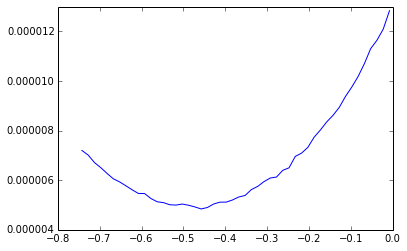
In all the cases, we can see that the variance ratio becomes very interesting when the option gets deeply out of the money and less significant, yet still very interesting, when the option is at or in the money. This corresponds to the natural behaviour of variance reduction techniques that involve measure changes, as the measure change is going to increase the probability of choosing a trajectory that is eventually going to enter the money. Note that the simulation time is only slightly larger when simulating with the measure change, while the time required for the optimization procedure is negligible compared with the simulation time. In Figure 6.1, we fix the maturity to T=1.5T=1.5 and plot the empirical variance of the estimator (6.8) as a function of θ\theta. Our method provides θ=−0.457\theta=-0.457 as asymptotically optimal measure change. We can therefore see that the asymptotically optimal θ\theta is very close to the optimal one.

Refer to caption
Figure 6.1. The variance of the Monte-Carlo estimator as a function of θ\theta.

6.1.2. Numerical results for Asian put options

We now consider the case of a (discretized) Asian put option. Here, the log-payoff is

H⁡(X)=log⁡(K−S0n​∑j=1neXtj)+,H(X)=\log\left(K-\frac{S_{0}}{n}\sum_{j=1}^{n}e^{X_{t_{j}}}\right)_{+}\>,

where tj=jn​Tt_{j}=\frac{j}{n}\,T. By Prop. 5.5, the support of θ\theta is {t1,…,tn}\{t_{1},...,t_{n}\} and we can denote θj=θ⁡({tj})\theta_{j}=\theta(\{t_{j}\}). Using Prop. 6.1 and eq. (6.5), the function that we need to minimize is

log⁡(K1−∑l=1nθl)−∑m=1nθm​log⁡(−θmnK/S01−∑l=1nθl)+Tn​∑j=1nh⁡(∑l=jnθl)\log\left(\frac{K}{1-\sum_{l=1}^{n}\theta_{l}}\right)-\sum_{m=1}^{n}\theta_{m}\log\left(\frac{-\theta_{m}\,n\,K/S_{0}}{1-\sum_{l=1}^{n}\theta_{l}}\right)+\frac{T}{n}\sum_{j=1}^{n}h\left(\sum_{l=j}^{n}\theta_{l}\right)

or, alternatively, denoting Θj=∑l=jnθl\Theta_{j}=\sum_{l=j}^{n}\theta_{l},

log⁡(K1−Θ1)−∑m=1n(Θm−Θm+1)​log⁡(−(Θm−Θm+1)nK/S01−Θ1)+Tn​∑j=1nh⁡(Θj).\log\left(\frac{K}{1-\Theta_{1}}\right)-\sum_{m=1}^{n}(\Theta_{m}-\Theta_{m+1})\log\!\left(\frac{-(\Theta_{m}\!-\Theta_{m+1})\,nK/S_{0}}{1-\Theta_{1}}\right)+\frac{T}{n}\sum_{j=1}^{n}h\left(\Theta_{j}\right)\>.

By differentiating with respect to Θj\Theta_{j}, we obtain, for j=2,…,nj=2,...,n,

(6.9) 0\displaystyle 0 =∂Θj{H^​(θ)+Tn​∑m=1nh⁡(Θm)}\displaystyle=\partial_{\Theta_{j}}\left\{\hat{H}(\theta)+\frac{T}{n}\sum_{m=1}^{n}h\left(\Theta_{m}\right)\right\}
=T​h′​(Θj)n−log⁡[−(Θj−Θj+1)]+log⁡[−(Θj−1−Θj)],\displaystyle=\frac{T\,h^{\prime}\left(\Theta_{j}\right)}{n}-\log\left[-(\Theta_{j}-\Theta_{j+1})\right]+\log\left[-(\Theta_{j-1}-\Theta_{j})\right]\>,

while, for j=1j=1, we have

(6.10) 0\displaystyle 0 =∂Θ1{H^​(θ)+Tn​∑m=1nh⁡(Θm)}\displaystyle=\partial_{\Theta_{1}}\left\{\hat{H}(\theta)+\frac{T}{n}\sum_{m=1}^{n}h\left(\Theta_{m}\right)\right\}
=\displaystyle= log⁡(1−Θ1)−log⁡(n​K/S0)+Tn​h′​(Θ1)−log⁡[−(Θ1−Θ2)].\displaystyle\log\left(1-\Theta_{1}\right)-\log(n\,K/S_{0})+\frac{T}{n}\,h^{\prime}\left(\Theta_{1}\right)-\log\left[-(\Theta_{1}-\Theta_{2})\right]\>.

Finally, taking the exponential in eqs. (6.9) and (6.10), we obtain

Θ2−Θ1\displaystyle\Theta_{2}-\Theta_{1\phantom{-1}} =(1−Θ1)​eTn​h′​(Θ1)⋅S0n​K\displaystyle=\>\>(1\phantom{\Theta_{n}\>}-\Theta_{1\phantom{-1}})\>\>e^{\frac{T}{n}\,h^{\prime}(\Theta_{1})}\cdot\frac{S_{0}}{n\,K}
Θ3−Θ2\displaystyle\Theta_{3}-\Theta_{2\phantom{-1}} =(Θ2−Θ1)​eTn​h′​(Θ2)\displaystyle=\>\>(\Theta_{2\phantom{-1}}-\Theta_{1\phantom{-1}})\>\>e^{\frac{T}{n}\,h^{\prime}(\Theta_{2})}
⋮\displaystyle\vdots\>\>\qquad =⋮\displaystyle=\qquad\qquad\vdots
Θn−Θn−1\displaystyle\Theta_{n}-\Theta_{n-1} =(Θn−1−Θn−2)​eTn​h′​(Θn−1)\displaystyle=\>\>(\Theta_{n-1}-\Theta_{n-2})\>\>e^{\frac{T}{n}\,h^{\prime}(\Theta_{n-1})}
−Θn\displaystyle-\Theta_{n\phantom{-1}} =(Θn−Θn−1)​eTn​h′​(Θn).\displaystyle=\>\>(\Theta_{n\phantom{-1}}-\Theta_{n-1})\>\>e^{\frac{T}{n}\,h^{\prime}(\Theta_{n})}\>.

Finally, define 𝒯\mathcal{T} the real function that associates to Θn\Theta_{n}

𝒯⁡(Θn)=(1−Θ1)​eTn​h′​(Θ1)⋅S0n​K−Θ2−Θ1,\mathcal{T}(\Theta_{n})=(1-\Theta_{1})\mathrm{e}^{\frac{T}{n}\,h^{\prime}(\Theta_{1})}\cdot\frac{S_{0}}{n\,K}-\Theta_{2}-\Theta_{1}\>,

where Θn−1=Θn+Θn​e−Tn​h′​(Θn)\Theta_{n-1}=\Theta_{n}+\Theta_{n}\,e^{-\frac{T}{n}\,h^{\prime}(\Theta_{n})} and iteratively,

Θj−2=Θj−1−(Θj−Θj−1)e−Tn​h′​(Θj−1),j=n,…,3.\Theta_{j-2}=\Theta_{j-1}-(\Theta_{j}-\Theta_{j-1})\,e^{-\frac{T}{n}\,h^{\prime}(\Theta_{j-1})}\>,\qquad j=n,...,3\>.

Equating 𝒯\mathcal{T} to 0 by dichotomy then gives the asymptotically optimal measure.
Again, we simulate N=10000N=10000 trajectories of the Heston model with parameters λ=1.15\lambda=1.15, μ=0.04\mu=0.04, ζ=0.2\zeta=0.2, ρ=−0.4\rho=-0.4 and initial values V0=0.04V_{0}=0.04 and S0=1S_{0}=1, under both ℙ\mathbb{P}, eq. (6.2), and ℙθ\mathbb{P}_{\theta}, eq. (6.6), with n=200n=200 and tj=jn​Tt_{j}=\frac{j}{n}\,T, using a standard Euler scheme with 200 discretization steps. For the ℙ\mathbb{P}-realisations X(i)X^{(i)}, we calculate the Asian put price as

(6.11) 1N​∑j=1N(K−S0n​∑j=1neXtj(i))+\frac{1}{N}\sum_{j=1}^{N}\left(K-\frac{S_{0}}{n}\sum_{j=1}^{n}e^{X_{t_{j}}^{(i)}}\right)_{+}

and for the ℙθ\mathbb{P}_{\theta}-realisations X(i,θ)X^{(i,\theta)}, as

(6.12) eΦ⁡(t1,Θ1,…,Θn)+Ψ⁡(t1,Θ1,…,Θn)​V0N∑j=1Ne−∑j=1nθjXtj(i,θ)(K−S0n∑j=1neXtj(i))+.\frac{e^{\Phi\left(t_{1},\Theta_{1},...,\Theta_{n}\right)+\Psi\left(t_{1},\Theta_{1},...,\Theta_{n}\right)\,V_{0}}}{N}\sum_{j=1}^{N}e^{-\sum_{j=1}^{n}\theta_{j}\,X_{t_{j}}^{(i,\theta)}}\left(K-\frac{S_{0}}{n}\sum_{j=1}^{n}e^{X_{t_{j}}^{(i)}}\right)_{+}\>.

Again, each time, we compute the ℙθ\mathbb{P}_{\theta}-standard deviation and the adjusted and non-adjusted variance ratios. In Table 4, we fix maturity to T=1.5T=1.5 and let the strike KK vary between 0.60.6 and 1.31.3.

KK Price Std. error Var. ratio Adj. ratio Time, s
0.6 3.466 ⋅10−5\cdot 10^{-5} 4.13 ⋅10−6\cdot 10^{-6} 16.9 14.6 19.9
0.7 0.000562 2.60 ⋅10−5\cdot 10^{-5} 5.77 4.77 21.1
0.8 0.00414 9.64 ⋅10−5\cdot 10^{-5} 4.36 3.77 20.1
0.9 0.0185 0.00024 3.48 3.09 20.6
1 0.0558 0.00043 3.49 3.07 20.1
1.1 0.120 0.00057 3.69 3.20 20.1
1.2 0.206 0.00062 4.27 3.80 19.7
1.3 0.301 0.00059 5.30 4.41 21.0
Table 4. The variance ratio as function of the strike for the Asian put option. λ=1.15\lambda=1.15, μ=0.04\mu=0.04, ζ=0.2\zeta=0.2, ρ=−0.4\rho=-0.4, S0=1S_{0}=1, V0=0.04V_{0}=0.04, T=1.5T=1.5, N=10000N=10000, 200200 discretization steps.

The conclusion is the same as for the European put option. Indeed, the variance ratio explodes when the option moves away from the money. Due to the time-dependence of the measure change, the adjusted variance ratio is consistently around 13% below its non-adjusted version. The adjusted variance ratio remains however very interesting, with values above 3 around the money.

6.2. European put options in the Heston model with negative exponential jumps

We now consider the Heston model with negative exponential jumps

(6.13) d​Xt\displaystyle dX_{t} =(δ−Vt2)​d​t+Vt​d​Wt1+d​Jt,\displaystyle=\left(\delta-\frac{V_{t}}{2}\right)\,dt+\sqrt{V_{t}}\,dW_{t}^{1}+dJ_{t}\>, X0=0\displaystyle X_{0}=0
d​Vt\displaystyle dV_{t} =λ⁡(μ−Vt)​d​t+ζ​Vt​d​Wt2,\displaystyle=\lambda(\mu-V_{t})\,dt+\zeta\sqrt{V_{t}}\,dW_{t}^{2}\>, V0=V0\displaystyle V_{0}=V_{0}
d​⟨W1,W2⟩t=ρ​d​t,\displaystyle d\hskip-1.99168pt\left\langle W^{1},W^{2}\right\rangle_{t}=\rho\,dt\>,

where W1,W2W^{1},W^{2} are standard ℙ\mathbb{P}-Brownian motions and (Jt)t≥0(J_{t})_{t\geq 0} is an independent compound Poisson process with constant jump rate rr and jump distribution Neg-Exp​(α)\text{Neg-}\text{Exp}(\alpha), i.e. the Lévy measure of (Jt)t≥0(J_{t})_{t\geq 0} is ν(dx)=rαeα​x𝟙{x<0}dx\nu(dx)=r\,\alpha e^{\alpha x}\mathds{1}_{\{x<0\}}dx. The martingale condition on S=S0​eXS=S_{0}\,e^{X} imposes δ=rα+1\delta=\frac{r}{\alpha+1}. The Laplace transform of (Xt,Vt)(X_{t},V_{t}) is

I​E​(eu​Xt+w​Vt)=eϕ⁡(t,u,w)+ψ⁡(t,u,w)​V0+u​X0,\mathrm{I\kern-1.99997ptE}\left(e^{uX_{t}+wV_{t}}\right)=e^{\phi(t,u,w)+\psi(t,u,w)V_{0}+uX_{0}}\>,

where ϕ,ψ\phi,\psi satisfy the Riccati equations

(6.14) ∂tϕ⁡(t,u,w)\displaystyle\partial_{t}\phi(t,u,w) =F⁡(u,ψ⁡(t,u,w))\displaystyle=F(u,\psi(t,u,w))\quad ϕ⁡(0,u,w)=0\displaystyle\phi(0,u,w)=0
∂tψ⁡(t,u,w)\displaystyle\partial_{t}\psi(t,u,w) =R⁡(u,ψ⁡(t,u,w))\displaystyle=R(u,\psi(t,u,w))\quad ψ⁡(0,u,w)=w\displaystyle\psi(0,u,w)=w

for F⁡(u,w)=λ​μ​w+κ~​(u)F(u,w)=\lambda\mu\,w+\tilde{\kappa}(u), where κ~​(u)=r​u​(u−1)(α+1)​(α+u)\tilde{\kappa}(u)=\frac{ru(u-1)}{(\alpha+1)(\alpha+u)}, and

R⁡(u,w)=ζ22​w2+ζ​ρ​u​w−λ​w+12​(u2−u).R(u,w)=\frac{\zeta^{2}}{2}\,w^{2}+\zeta\rho\,uw-\lambda w+\frac{1}{2}(u^{2}-u)\>.

Again, a standard calculation shows that the solution of the generalized Riccati equations (6.14) is

(6.15) ψ⁡(t,u,w)\displaystyle\psi(t,u,w) =1ζ​(λζ−ρ​u)−γζ2​tanh⁡(γ2​t)+η1+η​tanh⁡(γ2​t)\displaystyle=\frac{1}{\zeta}\left(\frac{\lambda}{\zeta}-\rho u\right)-\frac{\gamma}{\zeta^{2}}\,\frac{\tanh\left(\frac{\gamma}{2}\,t\right)+\eta}{1+\eta\,\tanh\left(\frac{\gamma}{2}\,t\right)}
ϕ⁡(t,u,w)\displaystyle\phi(t,u,w) =μ​λζ​(λζ−ρ​u)​t−2​μ​λζ2​log⁡(cosh⁡(γ2​t)+η​sinh⁡(γ2​t))+t​κ~​(u),\displaystyle=\mu\,\frac{\lambda}{\zeta}\left(\frac{\lambda}{\zeta}-\rho u\right)t-2\mu\frac{\lambda}{\zeta^{2}}\,\log\!\left(\cosh\left(\frac{\gamma}{2}t\right)+\eta\,\sinh\left(\frac{\gamma}{2}t\right)\right)\!+t\tilde{\kappa}(u)\>,

where γ=γ⁡(u)=ζ​(λζ−ρ​u)2+14−(u−12)2\gamma=\gamma(u)=\zeta\,\sqrt{\left(\frac{\lambda}{\zeta}-\rho u\right)^{2}\!\!+\frac{1}{4}-\!\left(u-\frac{1}{2}\right)^{2}} and η=η⁡(u,w)=λ−ζ​ρ​u−ζ2​wγ⁡(u)\eta=\eta(u,w)=\frac{\lambda-\zeta\rho u-\zeta^{2}w}{\gamma(u)}. Furthermore, for the Heston model with negative jumps, the function hh is given by

(6.16) h⁡(u)=μ​λζ​(λζ−ρ​u)−μ​λζ2​γ​(u)+κ~​(u).h(u)=\mu\,\frac{\lambda}{\zeta}\left(\frac{\lambda}{\zeta}-\rho u\right)-\mu\,\frac{\lambda}{\zeta^{2}}\,\gamma(u)+\tilde{\kappa}(u)\>.

Let us now study the effect of the Esscher transform on the dynamics of the Heston model with jumps.

Proposition 6.6.

Let ℙθ\mathbb{P}_{\theta} be the measure given by

d​ℙθd​ℙ=eθ​XTI​E​[eθ​XT].\frac{d\mathbb{P}_{\theta}}{d\mathbb{P}}=\frac{e^{\theta\,X_{T}}}{\mathrm{I\kern-1.99997ptE}\left[e^{\theta\,X_{T}}\right]}\>.

Under ℙθ\mathbb{P}_{\theta}, the dynamics of the ℙ\mathbb{P}-Heston process with jumps (Xt,Vt)(X_{t},V_{t}) becomes

(6.17) d​Xt\displaystyle dX_{t} =δ​d​t+(θ+ζ​ρ​ψ​(T−t,θ,0)−12)​Vt​d​t+Vt​d​W~t1+d​Jt,\displaystyle=\delta dt+\left(\theta+\zeta\rho\,\psi\left(T-t,\theta,0\right)-\frac{1}{2}\right)V_{t}\,dt+\sqrt{V_{t}}\,d\tilde{W}_{t}^{1}+dJ_{t}\>, X0=0\displaystyle X_{0}=0
d​Vt\displaystyle dV_{t} =λ~t​(μ~t−Vt)​d​t+ζ​Vt​d​W~t2,\displaystyle=\tilde{\lambda}_{t}\,(\tilde{\mu}_{t}-V_{t})\,dt+\zeta\sqrt{V_{t}}\,d\tilde{W}_{t}^{2}\>, V0=V0\displaystyle V_{0}=V_{0}
d​⟨W~1,W~2⟩t=ρ​d​t,\displaystyle d\hskip-1.99168pt\left\langle\tilde{W}^{1},\tilde{W}^{2}\right\rangle_{t}=\rho\,dt\>,

where W~\tilde{W} is 2-dimensional correlated ℙθ\mathbb{P}_{\theta}-Brownian motion, ϕ\phi and ψ\psi are given in (6.15),

λ~t=λ−ζ​θ​ρ−ζ2​ψ​(T−t,θ,0)andμ~t=λ​μλ~t\tilde{\lambda}_{t}=\lambda-\zeta\theta\rho-\zeta^{2}\,\psi\left(T-t,\theta,0\right)\quad\text{and}\quad\tilde{\mu}_{t}=\frac{\lambda\mu}{\tilde{\lambda}_{t}}

and (Jt)t≥0(J_{t})_{t\geq 0} is a compound Poisson process with jump rate r​αα+θ\frac{r\alpha}{\alpha+\theta} and jump distribution Neg-Exp​(α+θ)\text{Neg-Exp}(\alpha+\theta) under ℙθ\mathbb{P}_{\theta}.

Proof.

Denote

D⁡(t,Xt,Vt)=d​ℙθd​ℙ|ℱt=eϕ⁡(T−t,θ,0)eϕ⁡(T,θ,0)+ψ⁡(T,θ,0)​V0​eψ⁡(T−t,θ,0)​Vt+θ​Xt.D(t,X_{t},V_{t})=\left.\frac{d\mathbb{P}_{\theta}}{d\mathbb{P}}\right|_{\mathcal{F}_{t}}=\frac{e^{\phi\left(T-t,\theta,0\right)}}{e^{\phi\left(T,\theta,0\right)+\psi\left(T,\theta,0\right)\,V_{0}}}\>e^{\psi\left(T-t,\theta,0\right)\,V_{t}+\theta\,X_{t}}\>.

The dynamics of D⁡(t,Xt,Vt)D(t,X_{t},V_{t}) can then be expressed using Itō’s Lemma as

d​D​(t,Xt,Vt)\displaystyle dD(t,X_{t},V_{t}) =D⁡(t,Xt,Vt)​(θ​d​Xt+ψ⁡(T−t,θ,0)​d​Vt)+…​d​t\displaystyle=D(t,X_{t},V_{t})\left(\theta dX_{t}+\psi\left(T-t,\theta,0\right)dV_{t}\right)+...\,dt
=D⁡(t,Xt,Vt)​[Vt​(θ​d​Wt1+ζ​ψ​(T−t,θ,0)​d​Wt2)+θ⁡(δ​d​t+d​Jt)]\displaystyle=D(t,X_{t},V_{t})\!\left[\sqrt{V_{t}}\left(\theta dW_{t}^{1}\!+\!\zeta\,\psi\left(T\!\!-\!t,\theta,0\right)dW_{t}^{2}\right)\!+\!\theta\,(\delta dt\!+\!dJ_{t})\right]

and Girsanov’s theorem then shows that

d⁡(W~t1W~t2)=d⁡(Wt1Wt2)−Vt​(θ+ζ​ρ​ψ​(T−t,θ,0)θ​ρ+ζ​ψ​(T−t,θ,0))​d​td\left(\begin{array}[]{c}\tilde{W}_{t}^{1}\\ \tilde{W}_{t}^{2}\end{array}\right)=d\left(\begin{array}[]{c}W_{t}^{1}\\ W_{t}^{2}\end{array}\right)-\sqrt{V_{t}}\left(\begin{array}[]{c}\theta+\zeta\rho\,\psi\left(T-t,\theta,0\right)\\ \theta\rho+\zeta\,\psi\left(T-t,\theta,0\right)\end{array}\right)dt

is a 2-dimensional Brownian motion under the measure PθP_{\theta}. Replacing WW in eq. (6.2) by W~\tilde{W} gives eq. (6.17). In order to finish the proof, it remains to show that the jump process (Jt)t≥0(J_{t})_{t\geq 0} has the desired distribution under ℙθ\mathbb{P}_{\theta}. Let us calculate the ℙθ\mathbb{P}_{\theta}-Laplace transform of JtJ_{t}:

I​Eℙθ​[eu​Jt]\displaystyle\mathrm{I\kern-1.99997ptE}^{\mathbb{P}_{\theta}}\left[e^{uJ_{t}}\right] =I​E​[eu​Jt​I​E​[eθ​XT|ℱt]]I​E​[eθ​XT]\displaystyle=\frac{\mathrm{I\kern-1.99997ptE}\left[e^{uJ_{t}}\,\mathrm{I\kern-1.99997ptE}\left[e^{\theta X_{T}}\,\middle|\,\mathcal{F}_{t}\right]\right]}{\mathrm{I\kern-1.99997ptE}\left[e^{\theta X_{T}}\right]}
=eϕ⁡(T−t,θ,0)I​E​[eθ​XT]​I​E​[eu​Jt+ψ⁡(T−t,θ,0)​Vt+θ​Xt].\displaystyle=\frac{e^{\phi\left(T-t,\theta,0\right)}}{\mathrm{I\kern-1.99997ptE}\left[e^{\theta X_{T}}\right]}\mathrm{I\kern-1.99997ptE}\left[e^{uJ_{t}+\psi\left(T-t,\theta,0\right)\,V_{t}+\theta X_{t}}\right]\>.

By independence of the jumps,

I​E​[eu​Jt+ψ⁡(T−t,θ,0)​Vt+θ​Xt]=eθ​δ​t​I​E​[e(u+θ)​Jt]​I​E​[eψ⁡(T−t,θ,0)​Vt+θ⁡(Xt−δ​t−Jt)],\mathrm{I\kern-1.99997ptE}\left[e^{uJ_{t}+\psi\left(T-t,\theta,0\right)\,V_{t}+\theta X_{t}}\right]=e^{\theta\delta\,t}\,\mathrm{I\kern-1.99997ptE}\left[e^{(u+\theta)J_{t}}\right]\,\mathrm{I\kern-1.99997ptE}\left[e^{\psi\left(T-t,\theta,0\right)\,V_{t}+\theta(X_{t}-\delta\,t-J_{t})}\right]\>,

where I​E​[e(u+θ)​Jt]=e−r​t​u+θu+θ+α\mathrm{I\kern-1.99997ptE}\left[e^{(u+\theta)J_{t}}\right]=e^{-rt\frac{u+\theta}{u+\theta+\alpha}}. Furthermore, (Xt−δ​t−Jt,Vt)t≥0(X_{t}-\delta\,t-J_{t},\,V_{t})_{t\geq 0} is a standard Heston process without jumps. Therefore comparing (6.4) and (6.15), we find that

I​E​[eψ⁡(T−t,θ,0)​Vt+θ⁡(Xt−δ​t−Jt)]=eϕ⁡(t,θ,ψ⁡(T−t,θ,0))−t​r​θ​(θ−1)(α+1)​(α+θ)+ψ⁡(t,θ,ψ⁡(T−t,θ,0))​V0.\mathrm{I\kern-1.99997ptE}\left[e^{\psi\left(T-t,\theta,0\right)\,V_{t}+\theta(X_{t}-\delta\,t-J_{t})}\right]=e^{\phi(t,\theta,\psi\left(T-t,\theta,0\right))-t\frac{r\theta(\theta-1)}{(\alpha+1)(\alpha+\theta)}+\psi(t,\theta,\psi\left(T-t,\theta,0\right))\,V_{0}}\>.

Using the fact that ψ⁡(t,θ,ψ⁡(T−t,θ,0))=ψ⁡(T,θ,0)\psi(t,\theta,\psi\left(T-t,\theta,0\right))=\psi\left(T,\theta,0\right) and

ϕ⁡(T−t,θ,0)+ϕ⁡(t,θ,ψ⁡(T−t,θ,0))=ϕ⁡(T,θ,0)\phi\left(T-t,\theta,0\right)+\phi(t,\theta,\psi\left(T-t,\theta,0\right))=\phi\left(T,\theta,0\right)

(see eq. (2.1) in [Keller-Ressel, 2011]), we finally obtain

I​Eℙθ​[eu​Jt]\displaystyle\mathrm{I\kern-1.99997ptE}^{\mathbb{P}_{\theta}}\left[e^{uJ_{t}}\right] =eθ​δ​t−r​t​u+θu+θ+α−t​r​θ​(θ−1)(α+1)​(α+θ)\displaystyle=e^{\theta\delta\,t-rt\frac{u+\theta}{u+\theta+\alpha}-t\frac{r\theta(\theta-1)}{(\alpha+1)(\alpha+\theta)}}
=eθ​rα+1​t−r​t​u+θu+θ+α−t​r​θ​(θ−1)(α+1)​(α+θ)=e−r​αα+θ​t​uu+(α+θ),\displaystyle=e^{\theta\frac{r}{\alpha+1}\,t-rt\frac{u+\theta}{u+\theta+\alpha}-t\frac{r\theta(\theta-1)}{(\alpha+1)(\alpha+\theta)}}=e^{-\frac{r\alpha}{\alpha+\theta}\,t\,\frac{u}{u+(\alpha+\theta)}}\>,

which is indeed the Laplace transform of a compound Poisson process with jump rate r​αα+θ\frac{r\alpha}{\alpha+\theta} and Neg-Exp​(α+θ)\text{Neg-Exp}(\alpha+\theta)-distributed jumps. ∎

6.2.1. Numerical results for the European put option

Similarly to the case of the Heston model without jumps, denoting θ=θ⁡({T})\theta=\theta(\{T\}), we have

(6.18) H^​(θ)+∫0Th⁡(θ⁡([t,T]))​𝑑t\displaystyle\hat{H}(\theta)+\int_{0}^{T}h(\theta([t,T]))\,dt
=log⁡(K1−θ)−θ​log⁡(−θK/S01−θ)+T​μ​λζ​(λζ−ρ​θ−γ⁡(θ)ζ)+T​κ~​(θ)\displaystyle=\>\log\left(\frac{K}{1-\theta}\right)-\theta\log\left(\frac{-\theta\,K/S_{0}}{1-\theta}\right)+T\,\mu\,\frac{\lambda}{\zeta}\left(\frac{\lambda}{\zeta}-\rho\theta-\frac{\gamma(\theta)}{\zeta}\,\right)+T\,\tilde{\kappa}(\theta)

and we obtain the asymptotically optimal θ\theta by differentiating (6.18) with respect to θ\theta and equating the derivative to 0 by dichotomy .
We simulate N=10000N=10000 trajectories of the Heston model with jumps with parameters λ=1.1\lambda=1.1, μ=0.7\mu=0.7, ζ=0.3\zeta=0.3, ρ=−0.5\rho=-0.5, r=2r=2, α=3\alpha=3 and initial values V0=1.3V_{0}=1.3 and S0=1S_{0}=1, under both ℙ\mathbb{P}, eq. (6.13), and ℙθ\mathbb{P}_{\theta}, eq. (6.17), using a standard Euler scheme with 200 discretization steps. For the ℙ\mathbb{P}-realisations X(i)X^{(i)}, we calculate the standard Monte-Carlo estimator of the European put price and for the ℙθ\mathbb{P}_{\theta}-realisations X(i,θ)X^{(i,\theta)}, we use (6.8) where ϕ\phi and ψ\psi are given in (6.15) and compute the same statistics as in the previous examples. In Table 5, we fix the strike to the value K=1K=1 and let the maturity TT vary from 0.250.25 to 33, whereas in Tables 6 and 7, we fix the maturity to T=1T=1 and to T=3T=3, while we let the strike KK vary between 0.250.25 and 1.751.75.

TT Price Std. error Var. ratio Adj. ratio Time, s
0.25 0.0945 9.96 ⋅10−4\cdot 10^{-4} 3.28 3.00 23.6
0.5 0.147 1.28 ⋅10−3\cdot 10^{-3} 3.20 2.99 24.5
1 0.215 1.61 ⋅10−3\cdot 10^{-3} 2.95 2.77 24.7
2 0.309 2.04 ⋅10−3\cdot 10^{-3} 2.61 2.43 24.7
3 0.374 2.30 ⋅10−3\cdot 10^{-3} 2.40 2.20 25.0
Table 5. The variance ratio as function of the maturity for the European put option in the Heston model with jumps.
KK Price Std. error Var. ratio Adj. ratio Time, s
0.25 0.00606 7.83 ⋅10−5\cdot 10^{-5} 11.6 10.4 25.8
0.5 0.0377 4.03 ⋅10−4\cdot 10^{-4} 5.42 5.28 24.7
0.75 0.105 9.44 ⋅10−4\cdot 10^{-4} 3.76 3.19 27.3
1 0.215 1.61 ⋅10−3\cdot 10^{-3} 2.93 2.89 26.1
1.25 0.369 2.26 ⋅10−3\cdot 10^{-3} 2.65 2.46 25.4
1.5 0.550 2.80 ⋅10−3\cdot 10^{-3} 2.43 2.24 24.9
1.75 0.766 3.05 ⋅10−3\cdot 10^{-3} 2.57 2.44 24.6
Table 6. The variance ratio as function of the strike for the European put option with maturity T=1T=1 in the Heston model with jumps.
KK Price Std. error Var. ratio Adj. ratio Time, s
0.25 0.0280 2.69 ⋅10−4\cdot 10^{-4} 5.19 4.99 24.8
0.5 0.108 8.60 ⋅10−4\cdot 10^{-4} 3.32 3.05 25.1
0.75 0.226 1.58 ⋅10−3\cdot 10^{-3} 2.68 2.56 26.3
1 0.374 2.31 ⋅10−3\cdot 10^{-3} 2.39 2.20 27.0
1.25 0.545 3.01 ⋅10−3\cdot 10^{-3} 2.20 2.19 25.2
1.5 0.730 3.66 ⋅10−3\cdot 10^{-3} 2.09 1.94 24.6
1.75 0.932 4.27 ⋅10−3\cdot 10^{-3} 1.97 1.83 24.8
Table 7. The variance ratio as function of the strike for the European put option with maturity T=3T=3 in the Heston model with jumps.

When adding negative jumps to the Heston model, one can see that the variance ratio diminishes. When the options are out of the money however it is still sufficiently important to make it interesting to use in applications. In Figure 6.2, we fix the maturity to T=1.5T=1.5 and plot again the empirical variance of the estimator (6.8) as a function of θ\theta for the Heston model with jumps. The method provides θ=−0.312\theta=-0.312 as asymptotically optimal measure change which is, as in the continuous case, very close to the optimal one.
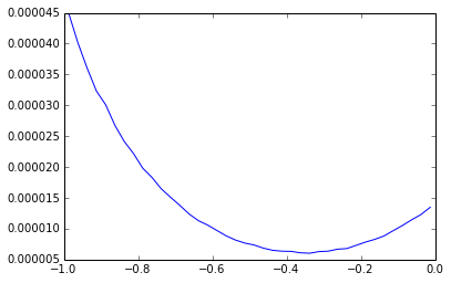
Refer to caption
Figure 6.2. The variance of the Monte-Carlo estimator as a function of θ\theta for the Heston model with jumps.

References

  • Barndorff-Nielsen, 1997 Barndorff-Nielsen, O. E. (1997). Processes of normal inverse Gaussian type. Finance and Stochastics, 2(1):41–68.
  • Barndorff-Nielsen and Shephard, 2001 Barndorff-Nielsen, O. E. and Shephard, N. (2001). Non-Gaussian Ornstein–Uhlenbeck-based models and some of their uses in financial economics. Journal of the Royal Statistical Society: Series B (Statistical Methodology), 63(2):167–241.
  • Bates, 1996 Bates, D. S. (1996). Jumps and stochastic volatility: Exchange rate processes implicit in Deutsche mark options. The Review of Financial Studies, 9(1):69–107.
  • Dembo and Zeitouni, 1998 Dembo, A. and Zeitouni, O. (1998). Large Deviations Techniques and Applications. Springer, Application of Mathematics, second edition.
  • Duffie et al., 2003 Duffie, D., Filipovic, D., and Schachermayer, W. (2003). Affine processes and applications in finance. The Annals of Applied Probability, 13(3):984–1053.
  • Dupuis and Wang, 2004 Dupuis, P. and Wang, H. (2004). Importance sampling, large deviations, and differential games. Stochastics: An International Journal of Probability and Stochastic Processes, 76(6):481–508.
  • Genin and Tankov, 2016 Genin, A. and Tankov, P. (2016). Optimal importance sampling for Lévy processes. Preprint, arXiv: 1608.04621.
  • Glasserman et al., 1999 Glasserman, P., Heidelberger, P., and Shahabuddin, P. (1999). Asymptotically optimal importance sampling and stratification for pricing path-dependent options. Mathematical Finance, 9(2):117–152.
  • Guasoni and Robertson, 2008 Guasoni, P. and Robertson, S. (2008). Optimal importance sampling with explicit formulas in continuous time. Finance and Stochastics, 12(1):1–19.
  • Heston, 1993 Heston, S. L. (1993). A closed-form solutions for options with stochastic volatility with applications to bond and currency options. Review of Financial Studies, 6(2):327–343.
  • Jacquier et al., 2013 Jacquier, A., Keller-Ressel, M., and Mijatović, A. (2013). Large deviations and stochastic volatility with jumps: asymptotic implied volatility for affine models. Stochastics: An International Journal of Probability and Stochastic Processes, 85(2):321–345.
  • Keller-Ressel, 2011 Keller-Ressel, M. (2011). Moment explosions and long-term behavior of affine stochastic volatility models. Mathematical Finance, 21(1):73–98.
  • Léonard, 2000 Léonard, C. (2000). Large deviations for Poisson random measures and processes with independent increments. Stochastic Processes and their Applications, 85(1):93–121.
  • Robertson, 2010 Robertson, S. (2010). Sample path large deviations and optimal importance sampling for stochastic volatility models. Stochastic Processes and their Applications, 120(1):66–83.
  • Rockafellar, 1971 Rockafellar, R. T. (1971). Integrals which are convex functionals. II. Pacific Journal of Mathematics, 39(2):439–469.