跳到论文正文
W Papers独立论文阅读器 arXiv:1809.06052 论文正文 计算阅读时间 · 0%
引用这篇论文根据当前论文元数据生成,正式投稿前建议核对。


License: arXiv.org perpetual non-exclusive license
arXiv:1809.06052v1 [stat.ME] 17 Sep 2018

∎

Parameter Estimation of four parameter absolute continuous Geometric Marshall-Olkin bivariate Pareto Distribution

Biplab Paul    Arabin Kumar Dey    Arjun K Gupta and Debasis Kundu E-mail: arabin@iitg.ac.in E-mail: gupta6731@gmail.com Affiliation: Department of Mathematics,
IIT Guwahati,
Guwahati, India


A. K. Dey Department of Mathematics,
IIT Guwahati,
Guwahati, India
Assam
Tel.: +91361-258-4620


Arjun K Gupta Department of Mathematics and Statistics,
Bowling Green State University, USA
E-mail: biplab.paul@iitg.ac.in Affiliation: Department of Mathematics,
IIT Guwahati,
Guwahati, India
E-mail: kundu@iitk.ac.in
Abstract

In this paper we formulate a four parameter absolute continuous Geometric Marshall-Olkin bivariate Pareto distribution and study its parameter estimation through EM algorithm and also explore the bayesian analysis through slice cum Gibbs sampler approach. Numerical results are shown to verify the performance of the algorithms. We illustrate the procedures through a real life data analysis.

Keywords: 
Joint probability density function, Absolute continuous bivariate Pareto distribution, EM algorithm, Geometric distribution, Slice Sampling.

1 Introduction

Geometric absolute continuous Marshall-Olkin bivariate Pareto (GBBVPA) is more flexible model than absolute continuous Marshall-Olkin bivariate Pareto. The distribution can be used to model data related to finance, insurance, environmental sciences and internet network. In this paper we explore the statistical inference of GBBVPA through EM algorithm. We also study bayesian analysis in this set up through slice cum Gibbs sampler approach. One of the required criteria for a data set which is to be used for modeling with GBBVPA should not have any equal components.

Kozubowski and Panorska (2008) and Barreto-Souza (2012), introduced geometric bivariate exponential and geometric bivariate gamma distributions, respectively, along the same line. Series of papers can also be found on statistical inferences on different distributions in the work of Kundu et al. [Kundu (2017), Kundu and Nekoukhou (2018) and Kundu and Gupta (2014)]. Few recent paper of Asimit et al [Asimit et al. (2016), Asimit et al. (2013), Asimit et al. (2010)] and Dey and Paul (2017) discussed statistical inference of singular bivariate Pareto with location scale parameter and its applications. Recently Dey and Paul [Dey and Paul (2017)] also studied singular four parameter Geometric Marshall Olkin bivariate Pareto distribution. However there is no paper available in statistical inference on absolute continuous Geometric Marshall-Olkin bivariate Pareto distribution. We also explore the bayesian analysis under informative prior. Both frequentist and bayesian confidence intervals are provided along with a illustrative real-life data example.

Maximum likelihood estimate may not only be computationally expensive, but also creat problems in finding suitable initial guesses. To resolve the issues we construct an EM algorithm. We also explore bayesian approach through slice cum gibbs sampler. Usual step-out procedure works quite well and easy to implement. Since it is a very flexible model when components are not equal, it gives the practitioner a choice of an alternative bivariate Pareto model, which may provide a better fit than existing Marshall-Olkin bivariate Pareto distribution.

Rest of paper is arranged as follows. In section 2 we show the formulation of Marshall-Olkin bivariate Pareto distribution. Section 3 discusses Maximum likelihood estimation through EM algorithm. Bayesian analysis is discussed in Section 4. Numerical results are shown in Section 5. Data analysis is shown for all methods in section 6. We conclude the paper in section 7.

2 Formulation of Block-Basu bivariate Pareto Geometric Distribution

2.1 Brief of singular Geometric bivariate Pareto Distribution

A bivariate random variable (X1,X2)(X_{1},X_{2}) is said to be distributed according to Marshall-Olkin bivariate Pareto distribution i.e., (X1,X2)∼M​O​B​V​P​A​(μ1,μ2,σ1,σ2,α0,α1,α2)(X_{1},X_{2})\sim MOBVPA(\mu_{1},\mu_{2},\sigma_{1},\sigma_{2},\alpha_{0},\alpha_{1},\alpha_{2}) if it has the cumulative survival function

S⁡(x1,x2)\displaystyle S(x_{1},x_{2}) =(1+z)−α0​(1+x1−μ1σ1)−α1​(1+x2−μ2σ2)−α2\displaystyle=(1+z)^{-\alpha_{0}}\Big(1+\frac{x_{1}-\mu_{1}}{\sigma_{1}}\Big)^{-\alpha_{1}}\Big(1+\frac{x_{2}-\mu_{2}}{\sigma_{2}}\Big)^{-\alpha_{2}}
={S1​(x1,x2),if x1−μ1σ1 <x2−μ2σ2S2​(x1,x2),if x1−μ1σ1 >x2−μ2σ2S0​(x),if x1−μ1σ1 = x2−μ2σ2=x\displaystyle=\begin{cases}S_{1}(x_{1},x_{2}),\quad\text{if $\frac{x_{1}-\mu_{1}}{\sigma_{1}}$ \textless$\frac{x_{2}-\mu_{2}}{\sigma_{2}}$}\\ S_{2}(x_{1},x_{2}),\quad\text{if $\frac{x_{1}-\mu_{1}}{\sigma_{1}}$ \textgreater$\frac{x_{2}-\mu_{2}}{\sigma_{2}}$}\\ S_{0}(x),\quad\text{if $\frac{x_{1}-\mu_{1}}{\sigma_{1}}$ = $\frac{x_{2}-\mu_{2}}{\sigma_{2}}$}=x\end{cases}

where

S1​(x1,x2)\displaystyle S_{1}(x_{1},x_{2}) =(1+x2−μ2σ2)−α0−α2​(1+x1−μ1σ1)−α1\displaystyle=\Big(1+\frac{x_{2}-\mu_{2}}{\sigma_{2}}\Big)^{-\alpha_{0}-\alpha_{2}}\Big(1+\frac{x_{1}-\mu_{1}}{\sigma_{1}}\Big)^{-\alpha_{1}}
S2​(x1,x2)\displaystyle S_{2}(x_{1},x_{2}) =(1+x2−μ2σ2)−α2​(1+x1−μ1σ1)−α0−α1\displaystyle=\Big(1+\frac{x_{2}-\mu_{2}}{\sigma_{2}}\Big)^{-\alpha_{2}}\Big(1+\frac{x_{1}-\mu_{1}}{\sigma_{1}}\Big)^{-\alpha_{0}-\alpha_{1}}
S0​(x)\displaystyle S_{0}(x) =(1+x)−α0−α1−α2\displaystyle=(1+x)^{-\alpha_{0}-\alpha_{1}-\alpha_{2}}

so it’s joint pdf can be written as

f⁡(x1,x2)\displaystyle f(x_{1},x_{2}) ={f1​(x1,x2),if x1−μ1σ1 <x2−μ2σ2f2​(x1,x2),if x1−μ1σ1 >x2−μ2σ2f0​(x),if x1−μ1σ1 = x2−μ2σ2=x\displaystyle=\begin{cases}f_{1}(x_{1},x_{2}),\quad\text{if $\frac{x_{1}-\mu_{1}}{\sigma_{1}}$ \textless$\frac{x_{2}-\mu_{2}}{\sigma_{2}}$}\\ f_{2}(x_{1},x_{2}),\quad\text{if $\frac{x_{1}-\mu_{1}}{\sigma_{1}}$ \textgreater$\frac{x_{2}-\mu_{2}}{\sigma_{2}}$}\\ f_{0}(x),\quad\text{if $\frac{x_{1}-\mu_{1}}{\sigma_{1}}$ = $\frac{x_{2}-\mu_{2}}{\sigma_{2}}$}=x\end{cases} (1)

where

f1​(x1,x2)\displaystyle f_{1}(x_{1},x_{2}) =α1​(α0+α2)σ1​σ2​(1+x2−μ2σ2)−α0−α2−1​(1+x1−μ1σ1)−α1−1\displaystyle=\frac{\alpha_{1}(\alpha_{0}+\alpha_{2})}{\sigma_{1}\sigma_{2}}\Big(1+\frac{x_{2}-\mu_{2}}{\sigma_{2}}\Big)^{-\alpha_{0}-\alpha_{2}-1}\Big(1+\frac{x_{1}-\mu_{1}}{\sigma_{1}}\Big)^{-\alpha_{1}-1}
f2​(x1,x2)\displaystyle f_{2}(x_{1},x_{2}) =α2​(α0+α1)σ1​σ2​(1+x2−μ2σ2)−α2−1​(1+x1−μ1σ1)−α0−α1−1\displaystyle=\frac{\alpha_{2}(\alpha_{0}+\alpha_{1})}{\sigma_{1}\sigma_{2}}\Big(1+\frac{x_{2}-\mu_{2}}{\sigma_{2}}\Big)^{-\alpha_{2}-1}\Big(1+\frac{x_{1}-\mu_{1}}{\sigma_{1}}\Big)^{-\alpha_{0}-\alpha_{1}-1}
f0​(x)\displaystyle f_{0}(x) =α0​(1+x)−α0−α1−α2−1\displaystyle=\alpha_{0}(1+x)^{-\alpha_{0}-\alpha_{1}-\alpha_{2}-1}

Suppose {(X1​i,X2​i):i=1,2,⋯}\{(X_{1i},X_{2i}):i=1,2,\cdots\} is a sequence of iid bivariate random variables with same cdf F⁡(⋅,⋅)F(\cdot,\cdot) and pdf f⁡(⋅,⋅)f(\cdot,\cdot). NN is an univariate random variable independent with (X1​n,X2​n)(X_{1n},X_{2n})’s follow Geometric distribution with 0<θ≤10<\theta\leq 1. We also consider that (Y1,Y2)(Y_{1},Y_{2}) is another bivariate random variable defined as,

Y1=min​{X11,X12,⋯,X1​N}Y_{1}=\text{min}\{X_{11},X_{12},\cdots,X_{1N}\}

Y2=min​{X21,X22,⋯,X2​N}Y_{2}=\text{min}\{X_{21},X_{22},\cdots,X_{2N}\}

The joint cumulative survival function can be obtained as,

G¯​(y1,y2)=θ​S​(y1,y2)1−(1−θ)​S​(y1,y2)\displaystyle\bar{G}(y_{1},y_{2})=\frac{\theta S(y_{1},y_{2})}{1-(1-\theta)S(y_{1},y_{2})} (2)

So it’s a joint density function that can be presented as,

g⁡(y1,y2)=θ⁡{1−(1−θ)​S​(y1,y2)}​∂2S⁡(y1,y2)∂y1​∂y2+2​θ​(1−θ)​∂S⁡(y1,y2)∂y1​∂S⁡(y1,y2)∂y2{1−(1−θ)​S​(y1,y2)}3\displaystyle g(y_{1},y_{2})=\frac{\theta\{1-(1-\theta)S(y_{1},y_{2})\}\partialderivative{S(y_1, y_2)}{y_1}{y_2}+2\theta(1-\theta)\partialderivative{S(y_1, y_2)}{y_1}\partialderivative{S(y_1, y_2)}{y_2}}{\{1-(1-\theta)S(y_{1},y_{2})\}^{3}} (3)

Now we use the survival function of MOBVPA in equation-3, then the joint distribution of (Y1,Y2)(Y_{1},Y_{2}) is called Geometric Marshall-Olkin bivariate Pareto (G-MOBVPA) distribution. Therefore the joint survival function of (Y1,Y2)(Y_{1},Y_{2}) can be written as,

G¯​(y1,y2)\displaystyle\bar{G}(y_{1},y_{2}) ={G¯1​(y1,y2),if y1−μ1σ1 <y2−μ2σ2G¯2​(y1,y2),if y1−μ1σ1 >y2−μ2σ2G¯0​(y),if y1−μ1σ1 = y2−μ2σ2\displaystyle=\begin{cases}\bar{G}_{1}(y_{1},y_{2}),\quad\text{if $\frac{y_{1}-\mu_{1}}{\sigma_{1}}$ \textless$\frac{y_{2}-\mu_{2}}{\sigma_{2}}$}\\ \bar{G}_{2}(y_{1},y_{2}),\quad\text{if $\frac{y_{1}-\mu_{1}}{\sigma_{1}}$ \textgreater$\frac{y_{2}-\mu_{2}}{\sigma_{2}}$}\\ \bar{G}_{0}(y),\quad\text{if $\frac{y_{1}-\mu_{1}}{\sigma_{1}}$ = $\frac{y_{2}-\mu_{2}}{\sigma_{2}}$}\\ \end{cases} (4)

where

G¯1​(y1,y2)\displaystyle\bar{G}_{1}(y_{1},y_{2}) =θ​(1+y1−μ1σ1)−α1​(1+y2−μ2σ2)−α0−α21−(1−θ)​(1+y1−μ1σ1)−α1​(1+y2−μ2σ2)−α0−α2\displaystyle=\frac{\theta\big(1+\frac{y_{1}-\mu_{1}}{\sigma_{1}}\big)^{-\alpha_{1}}\big(1+\frac{y_{2}-\mu_{2}}{\sigma_{2}}\big)^{-\alpha_{0}-\alpha_{2}}}{1-(1-\theta)\big(1+\frac{y_{1}-\mu_{1}}{\sigma_{1}}\big)^{-\alpha_{1}}\big(1+\frac{y_{2}-\mu_{2}}{\sigma_{2}}\big)^{-\alpha_{0}-\alpha_{2}}}
G¯2​(y1,y2)\displaystyle\bar{G}_{2}(y_{1},y_{2}) =θ​(1+y1−μ1σ1)−α0−α1​(1+y2−μ2σ2)−α21−(1−θ)​θ​(1+y1−μ1σ1)−α0−α1​(1+y2−μ2σ2)−α2\displaystyle=\frac{\theta\big(1+\frac{y_{1}-\mu_{1}}{\sigma_{1}}\big)^{-\alpha_{0}-\alpha_{1}}\big(1+\frac{y_{2}-\mu_{2}}{\sigma_{2}}\big)^{-\alpha_{2}}}{1-(1-\theta)\theta\big(1+\frac{y_{1}-\mu_{1}}{\sigma_{1}}\big)^{-\alpha_{0}-\alpha_{1}}\big(1+\frac{y_{2}-\mu_{2}}{\sigma_{2}}\big)^{-\alpha_{2}}}
G¯0​(y)\displaystyle\bar{G}_{0}(y) =θ​(1+y)−α0−α1−α21−(1−θ)​(1+y)−α0−α1−α2\displaystyle=\frac{\theta(1+y)^{-\alpha_{0}-\alpha_{1}-\alpha_{2}}}{1-(1-\theta)(1+y)^{-\alpha_{0}-\alpha_{1}-\alpha_{2}}}

Hence the joint pdf is,

g⁡(y1,y2)\displaystyle g(y_{1},y_{2}) ={g1​(y1,y2),if y1−μ1σ1 <y2−μ2σ2g2​(y1,y2),if y1−μ1σ1 >y2−μ2σ2g0​(y),if y1−μ1σ1 = y2−μ2σ2=y\displaystyle=\begin{cases}g_{1}(y_{1},y_{2}),\quad\text{if $\frac{y_{1}-\mu_{1}}{\sigma_{1}}$ \textless$\frac{y_{2}-\mu_{2}}{\sigma_{2}}$}\\ g_{2}(y_{1},y_{2}),\quad\text{if $\frac{y_{1}-\mu_{1}}{\sigma_{1}}$ \textgreater$\frac{y_{2}-\mu_{2}}{\sigma_{2}}$}\\ g_{0}(y),\quad\text{if $\frac{y_{1}-\mu_{1}}{\sigma_{1}}$ = $\frac{y_{2}-\mu_{2}}{\sigma_{2}}$}=y\end{cases} (5)

where

g1​(y1,y2)\displaystyle g_{1}(y_{1},y_{2}) =θ​α1​(α0+α2)​(1+y1−μ1σ1)−α1−1​(1+y2−μ2σ2)−α0−α2−1​{1+(1−θ)​S1​(y1,y2)}σ1​σ2​{1−(1−θ)​S1​(y1,y2)}3\displaystyle=\frac{\theta\alpha_{1}(\alpha_{0}+\alpha_{2})\big(1+\frac{y_{1}-\mu_{1}}{\sigma_{1}}\big)^{-\alpha_{1}-1}\big(1+\frac{y_{2}-\mu_{2}}{\sigma_{2}}\big)^{-\alpha_{0}-\alpha_{2}-1}\{1+(1-\theta)S_{1}(y_{1},y_{2})\}}{\sigma_{1}\sigma_{2}\{1-(1-\theta)S_{1}(y_{1},y_{2})\}^{3}}
g2​(y1,y2)\displaystyle g_{2}(y_{1},y_{2}) =θ⁡(α0+α1)​α2​(1+y1−μ1σ1)−α0−α1−1​(1+y2−μ2σ2)−α2−1​{1+(1−θ)​S2​(y1,y2)}σ1​σ2​{1−(1−θ)​S2​(y1,y2)}3\displaystyle=\frac{\theta(\alpha_{0}+\alpha_{1})\alpha_{2}\big(1+\frac{y_{1}-\mu_{1}}{\sigma_{1}}\big)^{-\alpha_{0}-\alpha_{1}-1}\big(1+\frac{y_{2}-\mu_{2}}{\sigma_{2}}\big)^{-\alpha_{2}-1}\{1+(1-\theta)S_{2}(y_{1},y_{2})\}}{\sigma_{1}\sigma_{2}\{1-(1-\theta)S_{2}(y_{1},y_{2})\}^{3}}
g0​(y)\displaystyle g_{0}(y) =θ​α0​(1+y)−α0−α1−α2−1{1−(1−θ)​(1+y)−α0−α1−α2}2\displaystyle=\frac{\theta\alpha_{0}(1+y)^{-\alpha_{0}-\alpha_{1}-\alpha_{2}-1}}{\{1-(1-\theta)(1+y)^{-\alpha_{0}-\alpha_{1}-\alpha_{2}}\}^{2}}

We denote this distribution as G−M​O​B​V​P​A​(θ,μ1,μ2,σ1,σ2,α0,α1,α2)G-MOBVPA(\theta,\mu_{1},\mu_{2},\sigma_{1},\sigma_{2},\alpha_{0},\alpha_{1},\alpha_{2}). From Lebesgue decomposition theorem, the joint pdf of (Y1,Y2)(Y_{1},Y_{2}) can be written as,

g⁡(y1,y2)\displaystyle g(y_{1},y_{2}) =α1+α2α0+α1+α2​ga​c​(y1,y2)+α0α0+α1+α2​gs​(y)\displaystyle=\frac{\alpha_{1}+\alpha_{2}}{\alpha_{0}+\alpha_{1}+\alpha_{2}}g_{ac}(y_{1},y_{2})+\frac{\alpha_{0}}{\alpha_{0}+\alpha_{1}+\alpha_{2}}g_{s}(y) (6)

where ga​c​(y1,y2)g_{ac}(y_{1},y_{2}) and gs​(y1,y2)g_{s}(y_{1},y_{2}) are the absolute continuous part and singular part of G-MOBVPA distribution. Here we are interested in absolute continuous part only.

2.2 Absolute continuous Geometric Marshall-Olkin bivariate Pareto distribution (G-BBBVPA)

In this paper we are interested in parameter estimation of absolute continuous part only. We consider the case when μ1=0\mu_{1}=0, μ2=0\mu_{2}=0, σ1=1\sigma_{1}=1 and σ2=1\sigma_{2}=1. We call the distribution as four parameter Geometric Block-Basu bivariate Pareto distribution and denote this as G−B​B​B​V​P​A​(θ,α0,α1,α2)G-BBBVPA(\theta,\alpha_{0},\alpha_{1},\alpha_{2}). Then the joint density function of (Y1,Y2)(Y_{1},Y_{2}) becomes,

g⁡(y1,y2)\displaystyle g(y_{1},y_{2}) ={p​θ​α1​(α0+α2)​(1+y1)−α1−1​(1+y2)−α0−α2−1​{1+(1−θ)​(1+y1)−α1​(1+y2)−α0−α2}{1−(1−θ)​(1+y1)−α1​(1+y2)−α0−α2}3,if y1 <y2p​θ​(α0+α1)​α2​(1+y1)−α0−α1−1​(1+y2)−α2−1​{1+(1−θ)​(1+y1)−α0−α1​(1+y2)−α2}{1−(1−θ)​(1+y1)−α0−α1​(1+y2)−α2}3,if y1 >y2\displaystyle=\begin{cases}\frac{p\theta\alpha_{1}(\alpha_{0}+\alpha_{2})(1+y_{1})^{-\alpha_{1}-1}(1+y_{2})^{-\alpha_{0}-\alpha_{2}-1}\{1+(1-\theta)(1+y_{1})^{-\alpha_{1}}(1+y_{2})^{-\alpha_{0}-\alpha_{2}}\}}{\{1-(1-\theta)(1+y_{1})^{-\alpha_{1}}(1+y_{2})^{-\alpha_{0}-\alpha_{2}}\}^{3}},\quad\text{if $y_{1}$ \textless$y_{2}$}\\ \frac{p\theta(\alpha_{0}+\alpha_{1})\alpha_{2}(1+y_{1})^{-\alpha_{0}-\alpha_{1}-1}(1+y_{2})^{-\alpha_{2}-1}\{1+(1-\theta)(1+y_{1})^{-\alpha_{0}-\alpha_{1}}(1+y_{2})^{-\alpha_{2}}\}}{\{1-(1-\theta)(1+y_{1})^{-\alpha_{0}-\alpha_{1}}(1+y_{2})^{-\alpha_{2}}\}^{3}},\quad\text{if $y_{1}$ \textgreater$y_{2}$}\end{cases} (7)

where p=α0+α1+α2α1+α2p=\frac{\alpha_{0}+\alpha_{1}+\alpha_{2}}{\alpha_{1}+\alpha_{2}}. The probability density plot and corresponding contour plot of different parameter sets are provided in Figure-1 and Figure-2 respectively.

Refer to caption
Figure 1: Probability density plot and Contour Plot for the parameter values θ=0.20\theta=0.20, α0=0.10\alpha_{0}=0.10, α1=0.20\alpha_{1}=0.20 and α2=0.40\alpha_{2}=0.40
Refer to caption
Figure 2: Probability density plot and Contour Plot for the parameter values θ=0.80\theta=0.80, α0=4\alpha_{0}=4, α1=5\alpha_{1}=5 and α2=10\alpha_{2}=10

2.3 Marginal distributions

The marginal distributions are easy to obtain from the above bivariate distribution which can be given by,

G¯​(y1)\displaystyle\bar{G}(y_{1}) =p⁡[θ​(1+y1−μ1σ1)−α0−α11−(1−θ)​(1+y1−μ1σ1)−α0−α1−(1−1p)​θ​(1+y1−μ1σ1)−(α0+α1+α2)1−(1−θ)​(1+y1−μ1σ1)−(α0+α1+α2)],\displaystyle=p[\frac{\theta(1+\frac{y_{1}-\mu_{1}}{\sigma_{1}})^{-\alpha_{0}-\alpha_{1}}}{1-(1-\theta)(1+\frac{y_{1}-\mu_{1}}{\sigma_{1}})^{-\alpha_{0}-\alpha_{1}}}-(1-\frac{1}{p})\frac{\theta(1+\frac{y_{1}-\mu_{1}}{\sigma_{1}})^{-(\alpha_{0}+\alpha_{1}+\alpha_{2})}}{1-(1-\theta)(1+\frac{y_{1}-\mu_{1}}{\sigma_{1}})^{-(\alpha_{0}+\alpha_{1}+\alpha_{2})}}],
 if y1>μ1y_{1}>\mu_{1} (8)
G¯​(y2)\displaystyle\bar{G}(y_{2}) =p[θ​(1+y2−μ2σ2)−α0−α21−(1−θ)​(1+y2−μ2σ2)−α0−α2−(1−1p)θ​(1+y2−μ2σ2)−(α0+α1+α2)1−(1−θ)​(1+y2−μ2σ2)−(α0+α1+α2)]],\displaystyle=p[\frac{\theta(1+\frac{y_{2}-\mu_{2}}{\sigma_{2}})^{-\alpha_{0}-\alpha_{2}}}{1-(1-\theta)(1+\frac{y_{2}-\mu_{2}}{\sigma_{2}})^{-\alpha_{0}-\alpha_{2}}}-(1-\frac{1}{p})\frac{\theta(1+\frac{y_{2}-\mu_{2}}{\sigma_{2}})^{-(\alpha_{0}+\alpha_{1}+\alpha_{2})}}{1-(1-\theta)(1+\frac{y_{2}-\mu_{2}}{\sigma_{2}})^{-(\alpha_{0}+\alpha_{1}+\alpha_{2})}}]],
 if y2>μ2y_{2}>\mu_{2} (9)

where p=α0+α1+α2α1+α2p=\frac{\alpha_{0}+\alpha_{1}+\alpha_{2}}{\alpha_{1}+\alpha_{2}}.

3 Parameter estimation through EM algorithm

Let us consider I={(y11,y21),(y12,y22),⋯,(y1​m,y2​m)}I=\{(y_{11},y_{21}),(y_{12},y_{22}),\cdots,(y_{1m},y_{2m})\}, sample of size mm from four parameter G-BBBVPA distribution. Let us also assume that μ1\mu_{1}, μ2\mu_{2}, σ1\sigma_{1} and σ2\sigma_{2} are known. Now we use the following notation:

I1={i:y1​i<y2​i}I_{1}=\{i:y_{1i}<y_{2i}\}, I2={i:y1​i>y2​i}I_{2}=\{i:y_{1i}>y_{2i}\}

Also m1=|I1|m_{1}=|I_{1}|, m2=|I2|m_{2}=|I_{2}|, m=m1+m2m=m_{1}+m_{2}.

We assume this data corresponds to a fictitious singular distribution where cardinality of singular observation is m0m_{0}. We form the usual EM in singular set up first. Suppose we observe not only (Y1,Y2)(Y_{1},Y_{2}) but also the corresponding NN value. Hence the complete data would be of the form,

{(y11,y21,n1),(y12,y22,n2)⋯,(y1​m∗,y2​m∗,nm∗)}\{(y_{11},y_{21},n_{1}),(y_{12},y_{22},n_{2})\cdots,(y_{1m^{*}},y_{2m^{*}},n_{m^{*}})\}

Here m∗=m0+m1+m2m^{*}=m_{0}+m_{1}+m_{2}.

We can imagine the following three independent hidden random variables corresponding to (Y1,Y2)(Y_{1},Y_{2}),

{U0|N=n}∼P​A​(I​I)​(0,1,n​α0)\{U_{0}|N=n\}\sim PA(II)(0,1,n\alpha_{0})

{U1|N=n}∼P​A​(I​I)​(0,1,n​α1)\{U_{1}|N=n\}\sim PA(II)(0,1,n\alpha_{1})

{U2|N=n}∼P​A​(I​I)​(0,1,n​α2)\{U_{2}|N=n\}\sim PA(II)(0,1,n\alpha_{2})

Also it is well known that

{Y1|N=n}=min⁡{{U0|N=n},{U1|N=n}}\{Y_{1}|N=n\}=\min\{{\{U_{0}|N=n\},\{U_{1}|N=n\}}\}

{Y2|N=n}=min⁡{{U0|N=n},{U2|N=n}}\{Y_{2}|N=n\}=\min\{{\{U_{0}|N=n\},\{U_{2}|N=n\}}\}

Pseudo-likelihood function described in (Dey and Paul (2018)) can be obtained as :

Q\displaystyle Q =Lp​s​e​u​d​o​(θ,α0,α1,α2)\displaystyle=L_{pseudo}(\theta,\alpha_{0},\alpha_{1},\alpha_{2})
=(∑i∈I0ln⁡(ai)+2​∑i∈I1ln⁡(ai)+2​∑i∈I2ln⁡(ai))+(m0+u1​m1+w1​m2)​ln⁡(α0)\displaystyle=\Big(\sum_{i\in I_{0}}\ln(a_i)+2\sum_{i\in I_{1}}\ln(a_i)+2\sum_{i\in I_{2}}\ln(a_i)\Big)+(m_{0}+u_{1}m_{1}+w_{1}m_{2})\ln(\alpha_0)
+(m1+w2​m2)​ln⁡(α1)+(u2​m1+m2)​ln⁡(α2)−(∑i∈I0ln⁡(1+y1​i)+∑i∈I1∪I2ln⁡(1+y1​i)CLOSE\displaystyle+(m_{1}+w_{2}m_{2})\ln(\alpha_1)+(u_{2}m_{1}+m_{2})\ln(\alpha_2)-\Big(\sum_{i\in I_{0}}\ln(1 + y_{1i})+\sum_{i\in I_{1}\cup I_{2}}\ln(1 + y_{1i})
+∑i∈I1∪I2ln⁡(1+y2​i))−α0(∑i∈I0ailn⁡(1+y1​i)+∑i∈I1ailn⁡(1+y2​i)+∑i∈I2ailn⁡(1+y1​i))\displaystyle+\sum_{i\in I_{1}\cup I_{2}}\ln(1 + y_{2i})\Big)-\alpha_{0}\Big(\sum_{i\in I_{0}}a_{i}\ln(1 + y_{1i})+\sum_{i\in I_{1}}a_{i}\ln(1 + y_{2i})+\sum_{i\in I_{2}}a_{i}\ln(1 + y_{1i})\Big)
−α1​(∑i∈I0ai​ln⁡(1+y1​i)+∑i∈I1ai​ln⁡(1+y1​i)+∑i∈I2ai​ln⁡(1+y1​i))−α2​(∑i∈I0ai​ln⁡(1+y1​i)CLOSE\displaystyle-\alpha_{1}\Big(\sum_{i\in I_{0}}a_{i}\ln(1 + y_{1i})+\sum_{i\in I_{1}}a_{i}\ln(1 + y_{1i})+\sum_{i\in I_{2}}a_{i}\ln(1 + y_{1i})\Big)-\alpha_{2}\Big(\sum_{i\in I_{0}}a_{i}\ln(1 + y_{1i})
+∑i∈I1ailn⁡(1+y2​i)+∑i∈I2ailn⁡(1+y2​i))+m∗ln⁡(θ1−θ)+ln⁡(1−θ)(∑i∈I0ai+∑i∈I1ai\displaystyle+\sum_{i\in I_{1}}a_{i}\ln(1 + y_{2i})+\sum_{i\in I_{2}}a_{i}\ln(1 + y_{2i})\Big)+m^{*}\ln(\frac{\theta}{1 - \theta})+\ln(1 - \theta)\Big(\sum_{i\in I_{0}}a_{i}+\sum_{i\in I_{1}}a_{i}
+∑i∈I2ai)\displaystyle+\sum_{i\in I_{2}}a_{i}\Big) (10)

EM updates for the parameters θ\theta, α0\alpha_{0}, α1\alpha_{1} and α2\alpha_{2} are given as follows,

α^0(t+1)=m0+u1(t)​m1+w1(t)​m2∑i∈I0ai(t)​ln⁡(1+y1​i)+∑i∈I1ai(t)​ln⁡(1+y2​i)+∑i∈I2ai(t)​ln⁡(1+y1​i).\hat{\alpha}^{(t+1)}_{0}=\frac{m_{0}+u^{(t)}_{1}m_{1}+w^{(t)}_{1}m_{2}}{\sum_{i\in I_{0}}a^{(t)}_{i}\ln(1+y_{1i})+\sum_{i\in I_{1}}a^{(t)}_{i}\ln(1+y_{2i})+\sum_{i\in I_{2}}a^{(t)}_{i}\ln(1+y_{1i})}. (11)
α^1(t+1)=m1+w2(t)​m2∑i∈I0ai(t)​ln⁡(1+y1​i)+∑i∈I1ai(t)​ln⁡(1+y1​i)+∑i∈I2ai(t)​ln⁡(1+y1​i)\hat{\alpha}^{(t+1)}_{1}=\frac{m_{1}+w^{(t)}_{2}m_{2}}{\sum_{i\in I_{0}}a^{(t)}_{i}\ln(1+y_{1i})+\sum_{i\in I_{1}}a^{(t)}_{i}\ln(1+y_{1i})+\sum_{i\in I_{2}}a^{(t)}_{i}\ln(1+y_{1i})} (12)
α^2(t+1)=m2+u2(t)​m1∑i∈I0ai(t)​ln⁡(1+y1​i)+∑i∈I1ai(t)​ln⁡(1+y2​i)+∑i∈I2ai(t)​ln⁡(1+y2​i)\hat{\alpha}^{(t+1)}_{2}=\frac{m_{2}+u^{(t)}_{2}m_{1}}{\sum_{i\in I_{0}}a^{(t)}_{i}\ln(1+y_{1i})+\sum_{i\in I_{1}}a^{(t)}_{i}\ln(1+y_{2i})+\sum_{i\in I_{2}}a^{(t)}_{i}\ln(1+y_{2i})} (13)

and

θ^(t+1)=m∗∑i∈I0ai(t)+∑i∈I1ai(t)+∑i∈I2ai(t)\hat{\theta}^{(t+1)}=\frac{m^{*}}{\sum_{i\in I_{0}}a^{(t)}_{i}+\sum_{i\in I_{1}}a^{(t)}_{i}+\sum_{i\in I_{2}}a^{(t)}_{i}} (14)

where ai(t)=E[N|y1​i,y2​i]a^{(t)}_{i}=E[N|y_{1i},y_{2i}] is the conditional mean of NN given Y1=y1Y_{1}=y_{1} and Y2=y2Y_{2}=y_{2} at the step tt and u1(t),u2(t),w1(t)u^{(t)}_{1},u^{(t)}_{2},w^{(t)}_{1} and w2(t)w^{(t)}_{2} are posterior probabilities at time step tt.

Important Issues and Suggested Solutions :

We do not observe m0m_{0} and each of the observation U0U_{0} falling in I0I_{0}. We also do not know aia_{i} when observations are in I0I_{0}. One of the straight solution is to replace all unknown quantities by its estimate m~0\tilde{m}_{0}, b~0\tilde{b}_{0}, a~0​i\tilde{a}_{0i}. So we replace m0m_{0} and each of the observation U0U_{0} falling in I0I_{0} by it’s estimates m~0=(m1+m2)​α0α1+α2\tilde{m}_{0}=(m_{1}+m_{2})\frac{\alpha_{0}}{\alpha_{1}+\alpha_{2}} and b~0=E⁡[U0|U0<min⁡{U1,U2}]=1n⁡(α0+α1+α2)−1\tilde{b}_{0}=E[U_{0}|U_{0}<\min\{U_{1},U_{2}\}]=\frac{1}{n(\alpha_{0}+\alpha_{1}+\alpha_{2})-1} , where nn should be replaced by a~0​i\tilde{a}_{0i}. We also use a~0​i\tilde{a}_{0i} as the estimate of aia_{i} falling in I0I_{0}. This method is valid when a~0​i​(α0+α1+α2)>1\tilde{a}_{0i}(\alpha_{0}+\alpha_{1}+\alpha_{2})>1. To make this a valid method for any range of parameters, we estimate log⁡(1+U0)\log(1 + U_0) by b~0∗=E⁡[log⁡(1+U0)|log⁡(1+U0)<min⁡{log⁡(1+U1),log⁡(1+U2)}]=1n⁡(α0+α1+α2)\tilde{b}^{*}_{0}=E[\log(1 + U_0)|\log(1 + U_0)<\min\{\log(1 + U_1),\log(1 + U_2)\}]=\frac{1}{n(\alpha_{0}+\alpha_{1}+\alpha_{2})} instead of estimating U0U_{0}. Hence the modified EM estimates for the parameters θ\theta, α0\alpha_{0}, α1\alpha_{1} and α2\alpha_{2} of four parameter G-BBBVPA will look like,

a~0​i(t+1)=1+(1−θ^(t))e−1/a~(t)0​i1−(1−θ^(t))e−1/a~(t)0​i\tilde{a}^{(t+1)}_{0i}=\frac{1+(1-\hat{\theta}^{(t)})e^{-1/\tilde{a}^{(t)}_{0i}}}{1-(1-\hat{\theta}^{(t)})e^{-1/\tilde{a}^{(t)}_{0i}}} (15)
b~0∗(t+1)=1a~0​i(t+1)​(α^0(t)+α^1(t)+α^2(t))\tilde{b}^{*(t+1)}_{0}=\frac{1}{\tilde{a}^{(t+1)}_{0i}\Big(\hat{\alpha}^{(t)}_{0}+\hat{\alpha}^{(t)}_{1}+\hat{\alpha}^{(t)}_{2}\Big)} (16)
α^0(t+1)=m~0+u1(t)​m1+w1(t)​m2m~0​a~0​i(t+1)​b~0∗(t+1)+∑i∈I1ai(t)​ln⁡(1+y2​i)+∑i∈I2ai(t)​ln⁡(1+y1​i).\hat{\alpha}^{(t+1)}_{0}=\frac{\tilde{m}_{0}+u^{(t)}_{1}m_{1}+w^{(t)}_{1}m_{2}}{\tilde{m}_{0}\tilde{a}^{(t+1)}_{0i}\tilde{b}^{*(t+1)}_{0}+\sum_{i\in I_{1}}a^{(t)}_{i}\ln(1+y_{2i})+\sum_{i\in I_{2}}a^{(t)}_{i}\ln(1+y_{1i})}. (17)
α^1(t+1)=m1+w2(t)​m2m~0​a~0​i(t+1)​b~0∗(t+1)+∑i∈I1ai(t)​ln⁡(1+y1​i)+∑i∈I2ai(t)​ln⁡(1+y1​i)\hat{\alpha}^{(t+1)}_{1}=\frac{m_{1}+w^{(t)}_{2}m_{2}}{\tilde{m}_{0}\tilde{a}^{(t+1)}_{0i}\tilde{b}^{*(t+1)}_{0}+\sum_{i\in I_{1}}a^{(t)}_{i}\ln(1 + y_{1i})+\sum_{i\in I_{2}}a^{(t)}_{i}\ln(1 + y_{1i})} (18)
α^2(t+1)=m2+u2(t)​m1m~0​a~0​i(t+1)​b~0∗(t+1)+∑i∈I1ai(t)​ln⁡(1+y2​i)+∑i∈I2ai(t)​ln⁡(1+y2​i)\hat{\alpha}^{(t+1)}_{2}=\frac{m_{2}+u^{(t)}_{2}m_{1}}{\tilde{m}_{0}\tilde{a}^{(t+1)}_{0i}\tilde{b}^{*(t+1)}_{0}+\sum_{i\in I_{1}}a^{(t)}_{i}\ln(1 + y_{2i})+\sum_{i\in I_{2}}a^{(t)}_{i}\ln(1 + y_{2i})} (19)

and

θ^(t+1)=m~0+m1+m2m~0​a~0​i(t+1)​b~0∗(t+1)+∑i∈I1ai(t)+∑i∈I2ai(t)\hat{\theta}^{(t+1)}=\frac{\tilde{m}_{0}+m_{1}+m_{2}}{\tilde{m}_{0}\tilde{a}^{(t+1)}_{0i}\tilde{b}^{*(t+1)}_{0}+\sum_{i\in I_{1}}a^{(t)}_{i}+\sum_{i\in I_{2}}a^{(t)}_{i}} (20)

Therefore the algorithmic steps of final working version can be given as :

Algorithm 1 Final modified EM procedure for four parameter Geometric absolute continuous Marshall Olkin bivariate Pareto distribution
1:  Set initial α0\alpha_{0}, α1\alpha_{1}, α2\alpha_{2} and θ(i+1)\theta_{(i+1)} and aia_{i}.
2:  while Δ​Q/Q<t​o​l\Delta Q/Q<tol do
3:   Compute a~0​i(t+1)\tilde{a}^{(t+1)}_{0i} using α0(i)\alpha^{(i)}_{0}, α1(i)\alpha^{(i)}_{1}, α2(i)\alpha^{(i)}_{2}
4:   Compute b~0​i∗(t+1)\tilde{b}^{*(t+1)}_{0i} using a~0​i(t+1)\tilde{a}^{(t+1)}_{0i}, α0(i)\alpha^{(i)}_{0}, α1(i)\alpha^{(i)}_{1} and α2(i)\alpha^{(i)}_{2}.
5:   Compute u1(i)u^{(i)}_{1}, u2(i)u^{(i)}_{2}, w1(i)w^{(i)}_{1}, w2(i)w^{(i)}_{2}, m~0\tilde{m}_{0} from α0(i)\alpha^{(i)}_{0}, α1(i)\alpha^{(i)}_{1}, α2(i)\alpha^{(i)}_{2} and a~0​i(t+1)\tilde{a}^{(t+1)}_{0i}.
6:   Update α0(i+1)\alpha^{(i+1)}_{0}, α1(i+1)\alpha^{(i+1)}_{1}, α2(i+1)\alpha^{(i+1)}_{2} and θ(i+1)\theta^{(i+1)} using Equation (17), (18), (19) and (20).
7:   Calculate QQ for the new iterate.
8:  end while

4 Bayesian Estimation

We use slice cum Gibbs sampler technique to calculate the bayes estimate. Usual step out is easy to implement in case of informative prior which makes bayesian procedure also appealing for the practitioners. At each Gibbs sampling step we plan to use slice sampling to generate the sample from the posterior.

4.1 Prior Assumption

We assume that α0\alpha_{0}, α1\alpha_{1}, and α2\alpha_{2} are distributed according to the gamma distribution with shape parameters kik_{i} and scale parameters θi\theta_{i}, i.e.,

α0∼Γ⁡(k0,θ0)≡Gamma⁡(k0,θ0)\displaystyle\alpha_{0}\sim\Gamma(k_{0},\theta_{0})\equiv\mathrm{Gamma}(k_{0},\theta_{0})
α1∼Γ⁡(k1,θ1)≡Gamma⁡(k1,θ1)\displaystyle\alpha_{1}\sim\Gamma(k_{1},\theta_{1})\equiv\mathrm{Gamma}(k_{1},\theta_{1})
α2∼Γ⁡(k2,θ2)≡Gamma⁡(k2,θ2)\displaystyle\alpha_{2}\sim\Gamma(k_{2},\theta_{2})\equiv\mathrm{Gamma}(k_{2},\theta_{2}) (21)

The probability density function of the Gamma Distribution is given by,

fΓ​(x,k,θ)=1Γ⁡(k)​θk​xk−1​e−xθ\displaystyle f_{\Gamma}(x;k,\theta)=\frac{1}{\Gamma(k)\theta^{k}}x^{k-1}e^{-\frac{x}{\theta}}

Here Γ⁡(k)\Gamma(k) is the gamma function evaluated at kk.

Further, we assume that the geometric parameter θ\theta is distributed according to Beta distribution first kind with the parameters aa and bb

π⁡(θ)=1β⁡(a,b)​θa−1​(1−θ)b−1,θ∈[0,1]\displaystyle\pi(\theta)=\frac{1}{\beta(a,b)}\theta^{a-1}(1-\theta)^{b-1},\quad\theta\in[0,1] (22)

4.2 Posterior Distribution

We known Bayes estimate of an unknown parameter under the squared error loss function is the posterior mean of the corresponding parameter. But in this case it is not easy to calculate Bayes estimate of unknown model parameters θ\theta, α0\alpha_{0}, α1\alpha_{1} and α2\alpha_{2} in closed form. We propose slice cum Gibbs sampling procedure to generates sample from conditional posterior distribution. The log full conditional posterior distributions of θ\theta, α0\alpha_{0}, α1\alpha_{1} and α2\alpha_{2} are given by,

ln⁡(π⁡(θ∣α0,α1,α2,I))\displaystyle\ln(\pi(\theta\mid\alpha_0, \alpha_1, \alpha_2, I)) =L⁡(θ,α0,α1,α2)−ln⁡(β⁡(a,b))+(a−1)​ln⁡θ\displaystyle=L(\theta,\alpha_{0},\alpha_{1},\alpha_{2})-\ln(\beta(a, b))+(a-1)\ln\theta
+(b−1)​ln⁡(1−θ)\displaystyle+(b-1)\ln(1-\theta)
ln⁡(π⁡(α0∣θ,α1,α2,I))\displaystyle\ln(\pi(\alpha_0\mid\theta, \alpha_1, \alpha_2, I)) =L⁡(θ,α0,α1,α2)−ln⁡(Γ⁡(k0))−k0​ln⁡(θ0)\displaystyle=L(\theta,\alpha_{0},\alpha_{1},\alpha_{2})-\ln(\Gamma(k_0))-k_{0}\ln(\theta_0)
+(k0−1)​ln⁡α0−α0θ0\displaystyle+(k_{0}-1)\ln\alpha_{0}-\frac{\alpha_{0}}{\theta_{0}}
ln⁡(π⁡(α1∣θ,α0,α2,I))\displaystyle\ln(\pi(\alpha_1\mid\theta, \alpha_0, \alpha_2, I)) =L⁡(θ,α0,α1,α2)−ln⁡(Γ⁡(k1))−k1​ln⁡(θ1)\displaystyle=L(\theta,\alpha_{0},\alpha_{1},\alpha_{2})-\ln(\Gamma(k_1))-k_{1}\ln(\theta_1)
+(k1−1)​ln⁡α1−α1θ1\displaystyle+(k_{1}-1)\ln\alpha_{1}-\frac{\alpha_{1}}{\theta_{1}}

and

ln⁡(π⁡(α2∣θ,α0,α1,I))\displaystyle\ln(\pi(\alpha_2\mid\theta, \alpha_0,\alpha_1, I)) =L⁡(θ,α0,α1,α2)−ln⁡(Γ⁡(k2))−k2​ln⁡(θ2)\displaystyle=L(\theta,\alpha_{0},\alpha_{1},\alpha_{2})-\ln(\Gamma(k_2))-k_{2}\ln(\theta_2)
+(k2−1)​ln⁡α2−α2θ2\displaystyle+(k_{2}-1)\ln\alpha_{2}-\frac{\alpha_{2}}{\theta_{2}}

respectively.

5 Numerical Analysis

We use the software R 3.5.0 to calculate all estimate. The codes are run at IIT Guwahati computers with model : Intel(R) Core(TM) i5-6200U CPU 2.30GHz. The codes will be available on request to authors. Here we take two different set of parameters with two different sample size as n=450n=450 and n=1000n=1000 in both of the estimation technique.

5.1 EM Estimates:

For EM estimates, we generate sample from this distribution with different sample sizes (n=300,450,1000n=300,450,1000) for two different parameter sets to calculate average estimates (AE), mean squared error (MSE) and 95% parametric bootstrap confidence interval (CI) of the parameters based on 1000 replications. We also observe the average iteration number for each of the cases. We use different initial choice of the parameters for different parameter sets but it remains same for different sample size in EM algorithm. It is observed that all results are near about same with other initial choice within it’s usual range. We have used the stopping criterion as the relative difference of log-likelihood and pseudo log-likelihood at each of the iteration with stopping tolerance limit as 0.000010.00001. All MLE results are shown in Table-1, Table-2, Table-3, Table-4, Table-5 and Table-6 respectively. The simulation provides average estimates closer to the original parameter with low MSEs which indicates that the method works quite well even for moderate sample size.

EM Algorithm Parameter Sets θ\theta α0\alpha_{0} α1\alpha_{1} α2\alpha_{2} Average Estimates 0.1880 0.0896 0.1923 0.3802 Mean Squared Error 0.0031 0.0022 0.0041 0.0131 Confidence Interval [0.0824 0.2825] [0.0018 0.1976] [0.0863 0.3134] [0.1771 0.5822] Average Number of Iteration 251

Table 1: Average Estimates (AE), Mean Square Errors (MSE) and Confidence Intervals (CI) of four parameter G-BBBPA with parameters θ=0.20\theta=0.20, α0=0.1\alpha_{0}=0.1, α1=0.2\alpha_{1}=0.2, α2=0.4\alpha_{2}=0.4 and sample size n=300n=300

EM Algorithm Parameter Sets θ\theta α0\alpha_{0} α1\alpha_{1} α2\alpha_{2} Average Estimates 0.1891 0.0910 0.1926 0.3817 Mean Squared Error 0.0025 0.0017 0.0030 0.0100 Confidence Interval [0.0809 0.2647] [0.0230 0.1783] [0.0868 0.2861] [0.1759 0.5431] Average Number of Iteration 238

Table 2: Average Estimates (AE), Mean Square Errors (MSE) and Confidence Intervals (CI) of four parameter G-BBBPA with parameters θ=0.20\theta=0.20, α0=0.1\alpha_{0}=0.1, α1=0.2\alpha_{1}=0.2, α2=0.4\alpha_{2}=0.4 and sample size n=450n=450

EM Algorithm Parameter Sets θ\theta α0\alpha_{0} α1\alpha_{1} α2\alpha_{2} Average Estimates 0.1926 0.0939 0.1948 0.3884 Mean Squared Error 0.0014 0.0008 0.0016 0.0056 Confidence Interval [0.0812 0.2464] [0.0428 0.1480] [0.0870 0.2581] [0.1734 0.4929] Average Number of Iteration 225

Table 3: Average Estimates (AE), Mean Square Errors (MSE) and Confidence Intervals (CI) of four parameter G-BBBVPA with parameters θ=0.20\theta=0.20, α0=0.1\alpha_{0}=0.1, α1=0.2\alpha_{1}=0.2, α2=0.4\alpha_{2}=0.4 and sample size n=1000n=1000

EM Algorithm Parameter Sets θ\theta α0\alpha_{0} α1\alpha_{1} α2\alpha_{2} Average Estimates 0.8091 4.0329 5.0769 10.0932 Mean Squared Error 0.0085 1.8467 0.9753 2.1252 Confidence Interval [0.6355 0.9992] [1.4026 6.7785] [3.3735 7.1640] [7.3086 13.0668] Average Number of Iteration 316

Table 4: Average Estimates (AE), Mean Square Errors (MSE) and Confidence Intervals (CI) of four parameter G-BBBVPA with parameters θ=0.80\theta=0.80, α0=4\alpha_{0}=4, α1=5\alpha_{1}=5, α2=10\alpha_{2}=10 and sample size n=300n=300

EM Algorithm Parameter Sets θ\theta α0\alpha_{0} α1\alpha_{1} α2\alpha_{2} Average Estimates 0.8062 4.0274 5.0526 10.0416 Mean Squared Error 0.0062 1.1381 0.6251 1.3914 Confidence Interval [0.6628 0.9678] [1.8657 5.9532] [3.6413 6.6936] [7.7724 12.4351] Average Number of Iteration 285

Table 5: Average Estimates (AE), Mean Square Errors (MSE) and Confidence Intervals (CI) of four parameter G-BBBVPA with parameters θ=0.80\theta=0.80, α0=4\alpha_{0}=4, α1=5\alpha_{1}=5, α2=10\alpha_{2}=10 and sample size n=450n=450

EM Algorithm Parameter Sets θ\theta α0\alpha_{0} α1\alpha_{1} α2\alpha_{2} Average Estimates 0.8016 4.0276 5.0191 5.0191 Mean Squared Error 0.0029 0.5228 0.2727 0.6100 Confidence Interval [0.70491 0.9051] [2.5286 5.4450] [4.1197 6.0914] [8.5197 11.5006] Average Number of Iteration 253

Table 6: Average Estimates (AE), Mean Square Errors (MSE) and Confidence Intervals (CI) of four parameter G-BBBVPA with parameters θ=0.80\theta=0.80, α0=4\alpha_{0}=4, α1=5\alpha_{1}=5, α2=10\alpha_{2}=10 and sample size n=1000n=1000

For Bayesian Estimation:

We compute the average bayesian estimates (ABE) of unknown parameters and also the associated mean squared error (MSE), credible intervals (CI) and coverage probability (CP) of CIs based on proper priors with fixed hyper-parameters. Although the code is done based on one particular set of hyper-parameters, it may work for any set of hyper-parameters. In step out method of slice sampling we choose our width as one. However we cross check that the algorithm works for both larger and smaller choices of width. The confidence intervals are constructed directly using R package coda. All bayesian results are shown in Table-7, Table-8, Table-9, Table-10, Table-11 and Table-12 respectively. Results indicate that the method used in this case works really well even for moderate sample size. We use the following hyper-parameters a=0.70a=0.70, b=0.75b=0.75, k0=0.70k_{0}=0.70, θ0=0.75\theta_{0}=0.75, k1=0.70k_{1}=0.70, θ1=0.75\theta_{1}=0.75, k2=0.70k_{2}=0.70 and θ2=0.75\theta_{2}=0.75 for Gamma priors. We observe in simulation experiment that the method works for multiple different choices of hyper-parameters indicating that the algorithm is independent of the choice of the hyper-parameters.

Slice-cum-Gibbs Gamma Prior Parameter Sets θ\theta α0\alpha_{0} α1\alpha_{1} α2\alpha_{2} Starting Value 0.4794 0.8654 0.7781 0.5386 Average Estimates 0.2142 0.1001 0.2178 0.4252 Mean Squared Error 0.0014 0.0023 0.0020 0.0055 Credible Interval [0.1882 0.3577] [0.00001 0.1889] [0.1684 0.37901] [0.3296 0.6382] Coverage Probabilities 0.95 0.915 0.96 0.965

Table 7: Average Bayesian Estimates (ABE), Mean Square Errors (MSE), Credible Intervals (CI) and Coverage Probabilities (CP) of the parameters of four parameter G-BBBVPA with parameters θ=0.20\theta=0.20, α0=0.10\alpha_{0}=0.10, α1=0.20\alpha_{1}=0.20, α2=0.40\alpha_{2}=0.40 and sample size n=300n=300

Slice-cum-Gibbs Gamma Prior Parameter Sets θ\theta α0\alpha_{0} α1\alpha_{1} α2\alpha_{2} Starting Value 0.4794 0.8654 0.7781 0.5386 Average Estimates 0.2074 0.0987 0.2098 0.4130 Mean Squared Error 0.0008 0.0012 0.0015 0.0042 Credible Interval [0.1897 0.3264] [0.00001 0.1607] [0.1908 0.3614] [0.3281 0.5755] Coverage Probabilities 0.96 0.975 0.955 0.93

Table 8: Average Bayesian Estimates (ABE), Mean Square Errors (MSE), Credible Intervals (CI) and Coverage Probabilities (CP) of the parameters of four parameter G-BBBVPA with parameters θ=0.20\theta=0.20, α0=0.10\alpha_{0}=0.10, α1=0.20\alpha_{1}=0.20, α2=0.40\alpha_{2}=0.40 and sample size n=450n=450

Slice-cum-Gibbs Gamma Prior Parameter Sets θ\theta α0\alpha_{0} α1\alpha_{1} α2\alpha_{2} Starting Value 0.4794 0.8654 0.7781 0.5386 Average Estimates 0.2045 0.0970 0.2067 0.4086 Mean Squared Error 0.0004 0.0008 0.0007 0.0020 Credible Interval [0.1933 0.2797] [0.00829 0.1211] [0.1880 0.3019] [0.3691 0.5460] Coverage Probabilities 0.935 0.93 0.945 0.935

Table 9: Average Bayesian Estimates (ABE), Mean Square Errors (MSE), Credible Intervals (CI) and Coverage Probabilities (CP) of the parameters of four parameter G-BBBVPA with parameters θ=0.20\theta=0.20, α0=0.10\alpha_{0}=0.10, α1=0.20\alpha_{1}=0.20, α2=0.40\alpha_{2}=0.40 and sample size n=1000n=1000

Slice-cum-Gibbs Gamma Prior Parameter Sets θ\theta α0\alpha_{0} α1\alpha_{1} α2\alpha_{2} Starting Value 0.4794 0.8654 0.7781 0.5386 Average Estimates 0.6830 4.3083 3.9428 7.8710 Mean Squared Error 0.0197 1.2093 1.6216 5.9848 Credible Interval [0.6231 0.9841] [3.9782 9.0116] [2.0142 4.8029] [4.1524 9.1037] Coverage Probabilities 0.75 0.96 0.68 0.585

Table 10: Average Bayesian Estimates (ABE), Mean Square Errors (MSE), Credible Intervals (CI) and Coverage Probabilities (CP) of the parameters of four parameter G-BBBVPA with parameters θ=0.80\theta=0.80, α0=4\alpha_{0}=4, α1=5\alpha_{1}=5, α2=10\alpha_{2}=10 and sample size n=300n=300

Slice-cum-Gibbs Gamma Prior Parameter Sets θ\theta α0\alpha_{0} α1\alpha_{1} α2\alpha_{2} Starting Value 0.4794 0.8654 0.7781 0.5386 Average Estimates 0.7198 4.1272 4.3771 8.6477 Mean Squared Error 0.0120 0.9798 0.8628 2.9695 Credible Interval [0.7219 0.9996] [3.2084 7.2971] [3.0594 5.8116] [6.6313 11.0700] Coverage Probabilities 0.74 0.955 0.79 0.735

Table 11: Average Bayesian Estimates (ABE), Mean Square Errors (MSE), Credible Intervals (CI) and Coverage Probabilities (CP) of the parameters of four parameter G-BBBVPA with parameters θ=0.80\theta=0.80, α0=4\alpha_{0}=4, α1=5\alpha_{1}=5, α2=10\alpha_{2}=10 and sample size n=450n=450

Slice-cum-Gibbs Gamma Prior Parameter Sets θ\theta α0\alpha_{0} α1\alpha_{1} α2\alpha_{2} Starting Value 0.4794 0.8654 0.7781 0.5386 Average Estimates 0.7623 4.0852 4.7265 9.3589 Mean Squared Error 0.0043 0.4909 0.3335 0.9998 Credible Interval [0.6966 0.9068] [3.7685 6.3895] [3.1651 4.7518] [7.6523 10.3458] Coverage Probabilities 0.86 0.96 0.895 0.82

Table 12: Average Bayesian Estimates (ABE), Mean Square Errors (MSE), Credible Intervals (CI) and Coverage Probabilities (CP) of the parameters of four parameter G-BBBVPA with parameters θ=0.80\theta=0.80, α0=4\alpha_{0}=4, α1=5\alpha_{1}=5, α2=10\alpha_{2}=10 and sample size n=1000n=1000

6 Data Analysis

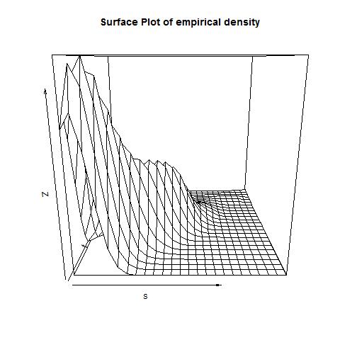
We use the same data set which is used by Paul Dey and Kundu (2018) for data analysis of three parameter BB-BVPA distribution. The data set is taken from https://archive.ics.uci.edu/ml/machine-learning-databases. The age of abalone is determined by cutting the shell through the cone, staining it, and counting the number of rings through a microscope. The data set contains related measurements. We extract a part of the data for bivariate modeling. We consider only measurements related to female population where one of the variable is Length as Longest shell measurement and other variable is Diameter which is perpendicular to length. We use peak over threshold method on this data set. It is observed that the transform data set doesn’t have any singular component. So instead of modeling with BBBVPA, we can plan to choose more generalized/flexible Geometric BBBVPA as one of the possible distributional assumption. We fit the empirical survival functions with the marginals of this distribution whose parameters are obtained from the both of proposed EM algorithm and Bayesian estimation. For the both marginals it has a good fit which are shown in Figure-4 and Figure-5 respectively for EM algorithms. We also verify our assumption by plotting empirical two dimensional density plot of this data which is shown in Figure-3.
Refer to caption
Figure 3: Two dimensional density plots of the transformed dataset

For EM algorithm:

The EM estimates of the parameters of four parameter BBBVPA based on transform data are θ=0.9999\theta=0.9999, α0=3.1388\alpha_{0}=3.1388, α1=1.7324\alpha_{1}=1.7324 and α2=1.5920\alpha_{2}=1.5920. Average estimates, mean square errors, confidence intervals and average number of iterations based on parametric bootstrap are available in Table-13.

Refer to caption
(a) For X1X_{1}
Refer to caption
(b) For X2X_{2}
Figure 4: Survival plots for two marginals through EM algorithm of the transformed dataset

EM Algorithm Parameter Sets θ\theta α0\alpha_{0} α1\alpha_{1} α2\alpha_{2} Average Estimates 0.9649 3.1298 1.6828 1.5462 Mean Squared Error 0.0040 0.3873 0.2126 0.1877 Confidence Interval [0.8226 0.9999] [1.9728 4.3470] [0.8174 2.6112] [0.7293 2.3890] Average Number of Iteration 1036

Table 13: Average Estimates (AE), Mean Square Errors (MSE) and Confidence Intervals (CI) of four parameter G-BBBVPA with parametersθ=0.9999\theta=0.9999, α0=3.1388\alpha_{0}=3.1388, α1=1.7324\alpha_{1}=1.7324, α2=1.5921\alpha_{2}=1.5921 and sample size n=329n=329

For Bayesian Estimation:

The Bayesian estimates of the parameters based on this data are θ=0.9852\theta=0.9852, α0=3.5395\alpha_{0}=3.5395, α1=1.3782\alpha_{1}=1.3782 and α2=1.2632\alpha_{2}=1.2632. We also calculate average bayesian estimates, mean squared error, credible intervals and coverage probability of the credible intervals using simulation technique which is available in Table-14.

Refer to caption
(a) For X1X_{1}
Refer to caption
(b) For X2X_{2}
Figure 5: Survival plots for two marginals through Bayesian Estimation of the transformed dataset

Slice-cum-Gibbs Gamma Prior Parameter Sets θ\theta α0\alpha_{0} α1\alpha_{1} α2\alpha_{2} Starting Value 0.4794 0.8654 0.7781 0.5386 Average Estimates 0.9067 3.3691 1.3061 1.1967 Mean Squared Error 0.0082 0.3280 0.1383 0.1175 Credible Interval [0.8637 1.000] [3.1685 5.5302] [0.0247 1.5164] [0.0213 1.4281] Coverage Probabilities 0.975 0.95 0.965 0.955

Table 14: Average Bayesian Estimates (ABE), Mean Square Errors (MSE), Credible Intervals (CI) and Coverage Probabilities (CP) of the parameters of four parameter G-BBBVPA with parameters θ=0.9852\theta=0.9852, α0=3.5395\alpha_{0}=3.5395, α1=1.3781\alpha_{1}=1.3781, α2=1.2632\alpha_{2}=1.2632 and sample size n=329n=329

7 Conclusion

We observe that it is a more flexible model than three parameter absolute continuous Marshall-Olkin bivariate Pareto distribution. We propose different modification while implementing the EM algorithm. Bayesian analysis through Slice cum Gibbs sampler is used for estimation of the parameters too. Modeling the data through G-MOBVPA may have more appeal for the practitioner when there is no equality in components of the model. However statistical inference for this model is much more difficult with location and scale due to its discontinuous nature of likelihood with respect to the parameters. A different alternative version of this Geometric distribution can also be proposed in the same direction. The work is on progress.

References

  • Asimit et al. (2010) Asimit, A. V., E. Furman, and R. Vernic (2010). On a multivariate pareto distribution. Insurance: Mathematics and Economics 46(2), 308–316.
  • Asimit et al. (2016) Asimit, A. V., E. Furman, and R. Vernic (2016). Statistical inference for a new class of multivariate pareto distributions. Communications in Statistics-Simulation and Computation 45(2), 456–471.
  • Asimit et al. (2013) Asimit, A. V., R. Vernic, and R. Zitikis (2013). Evaluating risk measures and capital allocations based on multi-losses driven by a heavy-tailed background risk: the multivariate pareto-ii model. Risks 1(1), 14–33.
  • Barreto-Souza (2012) Barreto-Souza, W. (2012). Bivariate gamma-geometric law and its induced lévy process. Journal of Multivariate Analysis 109, 130–145.
  • Dey and Paul (2017) Dey, A. K. and B. Paul (2017). Some variations of em algorithms for marshall-olkin bivariate pareto distribution with location and scale. arXiv preprint arXiv:1707.09974.
  • Dey and Paul (2018) Dey, A. K. and B. Paul (2018). Parameter estimation of four parameter geometric marshall-olkin bivariate pareto distribution. submitted.
  • Kozubowski and Panorska (2008) Kozubowski, T. J. and A. K. Panorska (2008). A mixed bivariate distribution connected with geometric maxima of exponential variables. Communications in Statistics—Theory and Methods 37(18), 2903–2923.
  • Kundu (2017) Kundu, D. (2017). Multivariate geometric skew-normal distribution. Statistics 51(6), 1377–1397.
  • Kundu and Gupta (2014) Kundu, D. and A. K. Gupta (2014). On bivariate weibull-geometric distribution. Journal of Multivariate Analysis 123, 19–29.
  • Kundu and Nekoukhou (2018) Kundu, D. and V. Nekoukhou (2018). Univariate and bivariate geometric discrete generalized exponential distributions. Journal of Statistical Theory and Practice, 1–20.