Extracting representations of cognition across neuroimaging
studies improves brain decoding
Arthur Mensch1*, Julien Mairal2, Bertrand Thirion1, Gaël Varoquaux1,
1 Inria, CEA, Univ. Paris Saclay, Paris, France
2 Univ. Grenoble Alpes, Inria, CNRS, Grenoble INP, LJK, Grenoble, France
* arthur.mensch@m4x.org
Abstract
Cognitive brain imaging is accumulating datasets about the neural substrate of many different mental processes. Yet, most studies are based on few subjects and have low statistical power. Analyzing data across studies could bring more statistical power; yet the current brain-imaging analytic framework cannot be used at scale as it requires casting all cognitive tasks in a unified theoretical framework. We introduce a new methodology to analyze brain responses across tasks without a joint model of the psychological processes. The method boosts statistical power in small studies with specific cognitive focus by analyzing them jointly with large studies that probe less focal mental processes. Our approach improves decoding performance for 80% of 35 widely-different functional-imaging studies. It finds commonalities across tasks in a data-driven way, via common brain representations that predict mental processes. These are brain networks tuned to psychological manipulations. They outline interpretable and plausible brain structures. The extracted networks have been made available; they can be readily reused in new neuro-imaging studies. We provide a multi-study decoding tool to adapt to new data.
Author summary
Brain-imaging findings in cognitive neuroscience often have low statistical power, despite the availability of functional imaging data across hundreds of studies. Yet, with current analytic frameworks, combining data across studies that map responses to different tasks discards the nuances of the cognitive questions they ask. In this paper, we propose a new approach for fMRI analysis, where a predictive model is used to extract the shared information from many studies together, while respecting their original paradigms. Our method extracts cognitive representations that associate a wide variety of functions to specific brain structures. This provides quantitative improvements and cognitive insights when analyzing together 35 task-fMRI studies; the breadth of the functional data we consider is much higher than in previous work. Reusing the representations learned by our approach also improves statistical power in studies outside the training corpus.
Introduction
Cognitive neuroscience uses functional brain imaging to probe the brain structures underlying mental processes. The field is accumulating neural activity responses to specific psychological manipulations. The diversity of studies that probe different mental processes gives a big picture on cognition [1]. However, as brain mapping has progressed in exploring finer aspects of mental processes, the statistical power of studies has stagnated or even decreased [2]—although sample size is increasing over years, it has not kept pace with the reduction of effect size. As a result, many, if not most individual studies often have low statistical power [3]. Large-scale efforts address this issue by collecting data from many subjects [4, 5]. For practical reasons, these efforts however focus on a small number of cognitive tasks. In contrast, establishing a complete view of the links between brain structures and the mental processes that they implement requires varied cognitive tasks [6], each crafted to recruit different mental processes. In this paper, we develop an analysis methodology that pools data across many task-fMRI studies to increase both statistical power and cognitive coverage. Standard meta analyses can only address commonalities across studies, as they require casting mental manipulations in a consistent overarching cognitive theory. They can bring statistical power at the cost of coverage and specificity in the cognitive processes. On the opposite, our approach uses the specific psychological manipulations of each study and extracts shared information from the brain responses across paradigms. As a result, it improves markedly the statistical power of mapping brain structures to mental processes. We demonstrate these benefits on 35 functional-imaging studies, all analyzed accordingly to their individual experimental paradigm.
Interpreting overlapping brain responses calls for multivariate analyses such as brain decoding [7]. Brain decoding uses machine learning to predict mental processes from the observed brain activity. It is a crucial tool to associate functions to given brain structures. Such inference endeavor calls for decoding across cognitive paradigms [8]. Indeed, a single study does not provide enough psychological manipulations to characterize well the functions of the brain structures that it activates [6], while covering a broader set of cognitive paradigms gives more precise functional descriptions. Moreover, the statistical power of functional data is limited by the sample size [3]. A single study seldom provides more than few hundreds of observations, which is well below machine-learning standards. Open repositories of brain functional images [9, 10] bring the hope of large-scale decoding with much larger sample sizes.
Yet, shoehorning such a diversity of studies into a decoding problem requires daunting manual annotation to build explicit correspondences across cognitive paradigms. We propose a different approach: we treat the decoding of each study as a single task in a multi-task linear decoding model [11, 12]. The parameters of this model are partially shared across studies to enable discovering potential commonalities. Model fitting—the training step of machine learning—is performed jointly, using non-convex training and regularization techniques [13, 14]. We thus learn to perform simultaneous decoding in many studies, to leverage the brain structures that they implicitly share. The extracted structures provide universal priors of functional mapping that improve decoding on new studies and can readily be reused in subsequent analyzes.
Models that generalize in measurable ways to new cognitive paradigms would ground broader pictures of cognition [15]. However, they face the fundamental roadblock that each cognitive study frames a particular question and resorts to specific task oppositions without clear counterpart in other studies [16]. In particular, a cognitive fMRI study results in contrast brain maps, each of which corresponds to an elementary psychological manipulation, often unique to a given protocol. Analyzing contrast maps across studies requires to model the relationships between protocols, which is a challenging problem. It has been tackled by labeling common aspects of psychological manipulations across studies, to build decoders that describe aspects of unseen paradigms [17, 18]. This annotation strategy is however difficult to scale up to a large set of studies as it requires expert knowledge on each study. The lack of complete cognitive ontologies to decompose psychological manipulations into mental processes [19] makes it even harder.
To overcome these obstacles, our multi-study decoding approach relies on the original labels of each study. Instead of relabeling data into a common ontology, the method extracts data-driven common cognitive dimensions. Our guiding hypothesis is that activation maps may be accurately decomposed into latent components that form the neural building blocks underlying cognitive processes [20]. This modelling overcomes the limitations of single-study cognitive subtraction models [19]. In particular, we show that it improves statistical power in individual studies: it gives better decoding performance for a vast majority of studies, and the improvement is particularly pronounced for studies with a small number of subjects. Our implicit modelling of functional information has the further advantage of providing explainable predictions. It decomposes the common aspects of psychological manipulations across studies onto latent factors, supported by spatial brain networks that are interpretable for neuroscience. These form by themselves a valuable resource for brain mapping: a functional atlas tuned to jointly decoding the cognitive information conveyed by various protocols. The trained model is a deep linear model. Building a linear model is important to bridge with classic decoding techniques in neuroimaging and ensures interpretability of intermediary representations.

Materials and methods
We first give an informal overview of the contributed methods for multi-study decoding. We review the mathematical foundations of the methods in a second part—a complete description is provided in S1A Appendix.. Finally, we describe how we validate the performance and usability of the approach. A preliminary version of our method was described in [21], with important differences and a less involved validation (S1B Appendix.).
| Study and task description | # contrasts | # subjects |
|---|---|---|
| [22] High level math & Localizer | 31 | 30 |
| [23] The ARCHI project | 30 | 78 |
| [24] Brainomics | 19 | 94 |
| [25] CamCAN | 5 | 605 |
| [26, 27] Music structure & Sentence structure | 19 | 35 |
| [28] Sentence/music complexity | 25 | 20 |
| [29] Balloon Analog Risk-taking | 12 | 16 |
| [30] Baseline trials & Classication learning | 7 | 17 |
| [31] Rhyme judgment | 3 | 13 |
| [32] Mixed-gambles | 4 | 16 |
| [33] Plain or mirror-reversed text | 9 | 14 |
| [34] Stop-signal | 6 | 20 |
| [35] Conditional stop-signal & Stop-signal | 12 | 13 |
| [36] Balloon analog risk task & Emotion regulation & Stop-signal & Temporal discounting task | 23 | 24 |
| [37] Classification probe without feedback & Dual-task weather classification & Single-task weather classification & Tone-counting | 14 | 14 |
| [38] Classification learning & Stop-signal | 11 | 8 |
| [38] Classification learning & Stop-signal | 11 | 8 |
| [39] Cross-language repetition priming | 17 | 13 |
| [40] Classification learning | 3 | 13 |
| [41] Simon task | 8 | 7 |
| [7] Visual object recognition | 13 | 6 |
| [42] Word & object processing | 6 | 49 |
| [43] Emotion regulation | 26 | 34 |
| [44] False belief | 7 | 36 |
| [45] Incidental encoding | 26 | 18 |
| [46] Covert verb generation & Line bisection & Motor & Overt verb generation & Overt word repetition | 11 | 10 |
| [47] Auditory oddball & Visual oddball | 8 | 17 |
| [48] Continuous house vs face & Discontinuous house (800ms) vs face & Discoutinuous house (400ms) vs face & House vs face | 30 | 11 |
| [48] Continuous house vs face & House vs face | 23 | 13 |
| [49] The Human Connectome Project | 23 | 786 |
| [50] Face recognition | 5 | 16 |
| [51] Arithmetic & Saccades | 26 | 19 |
| [52] UCLA LA5C consortium | 24 | 189 |
| [53] Foreign language & Localizer & Saccade | 34 | 65 |
| [54] Auditory compression & Visual compression | 14 | 16 |
| Total | 545 | 2343 |
Method overview
The approach has three main components, summarized in Fig 1: aggregating many fMRI studies, training a deep linear model, and reducing this model to extract interpretable intermediate representations. These representations are readily reusable to apply the methodology to new data. Building upon the increasing availability of public task-fMRI data, we gathered statistical maps from many task studies, along with rest-fMRI data from large repositories, to serve as training data for our predictive model (Fig 1A). Statistical maps are obtained by standard analysis, computing z-statistics maps for either base conditions, or for contrasts of interest when available. We use 40,000 subject-level contrast maps from 35 different studies (detailed in Table 1), with 545 different contrasts; a few are acquired in cohorts of hundreds of subjects (e.g., HCP, CamCan, LA5C), but most of them feature more common sample sizes of 10 to 20 subjects. These studies use different experimental paradigms, though most recruit related aspects of cognition (e.g., motor, attention, judgement tasks, object recognition).
We use machine-learning classification techniques for inter-subject decoding. Namely, we associate each brain activity contrast map with a predicted contrast class, chosen among the contrasts of the map’s study. For this, we propose a linear classification model featuring three layers of transformation (Fig 1B). This architecture reflects our working hypothesis: cognition can be represented on basic functions distributed spatially in the brain. The first layer projects contrast maps onto functional units learned from resting-state data. This first dimension reduction should be interpreted as a projection of the brain signal onto small, smooth and connected brain regions, tuned to capture the resting-state brain signal with a fine grain. The second layer performs dimension reduction and outputs an embedding of the brain activity into features that are common across studies. The embedded data from each study are then classified into their respective contrast class using a study-specific classification output from the third layer, in a setting akin to multi-task learning (see [55] for a review).
The second layer and the third layer are jointly extracted from the task-fMRI data using regularized stochastic optimization. Namely, the shared brain representation is optimized simultaneously with the third layer that performs decoding for every study. In particular, we use dropout regularization [56] in the layered model and stochastic optimization [13] to obtain good out-of-sample performance.
Study-specific decoding is thus performed on a shared low-dimensional brain representation. This representation is supported on 128 different combinations of the first 465 functional units identified with resting-state data. These combinations form diffuse networks of brain regions, that we call multi-study task-optimized networks (MSTONs). MSTONs differ from the notion of brain networks in the neuroscience literature—the later are typically obtained using a low-rank factorization of resting-state data, with a much lower number of components () than what we use to extract the functional units of the first layer.
As we will show, projecting data onto MSTONs improves across-subject predictive accuracy, removing confounds while preserving the cognitive signal. Interpretability is guaranteed by the linearity of the model and a post-training identification of stable directions in the space of latent representations. These networks capture a general multi-study representation of the cognitive signal contained in statistical maps.
Mathematical modelling
Following this informal description, we now review the mathematical foundations of our decoding approach. The complete descriptions of the predictive models and of the training algorithms are provided in S1A Appendix..
We consider task-fMRI studies, that we use for functional decoding. In this setting, each study features subjects, for which we compute different contrasts maps, using the General Linear Model [57]. Masking them using a grey-mask filter in the MNI space, we obtain a set of -maps , in , that summarizes the effect on brain activations of the psychological conditions . The goal of functional decoding is to learn a predictor from -maps to psychological conditions, namely a function . This predictor will be evaluated on unseen subjects for validation.
Linear decoding with shared parameters.
In our setting, we couple the predictors by forcing them to share parameters. Each study corresponds to a classification task, and we cast the problem as multi-task learning (as first considered in [11]). For this, we consider a given -map in study . We compute the predicted psychological condition using a factorized linear model:
| (1) |
The matrix and contain the basis for performing two successive projection of the -map onto low-dimension spaces. Those parameters are shared over all studies and form the first and second layer of our model. The matrix and the bias vector are the parameters of a multi-class linear classification model that labels the projected map with a psychological condition within the study . Those parameters are specific to each study , and form the third layer of our model.
First layer training from resting-state data.
The first dimension reduction, contained in the matrix , is learned using external resting-state data, from the HCP project [4]. Voxel time-series are stacked in a data matrix (with millions brain-images), that is factorized so that , with non-negative and sparse (i.e. with mostly null coefficients). This forces the elements of to delineate localized functional units. We use a sparse non-negative matrix factorization objective [58] and a recent scalable matrix factorization algorithm [59] to learn , as detailed in S1A Appendix.. The non-negativity constraint allows to interpret functional units as a soft parcellation of the brain. We do not use additional spatial constraints, as non-negative sparse matrix factorization with components readily finds smooth connected regions.
Joint training of the second and third layer.
The matrix and the multiple matrices and intercepts are trained jointly to minimize the objective
| (2) |
where is the standard -regularized multinomial loss function for training a linear model with classes (see S1A Appendix. for details). This objective is trained using Adam [13]; at each step, we select a batch of examples from one study. To prevent specialization of the rows of matrix to specific studies, we add a dropout noise [14] to the activations and during training.
Model consensus.
Although the atoms of are naturally interpretable, the fact that the product can always be rewritten as for an invertible matrix prevents us from directly identifying meaningful directions in the low-dimensional space spanned by . On the other hand, we found this space to be remarkably stable across training runs. We therefore propose an ensemble technique to extract a non-negative matrix such that captures meaningful directions (as above-mentioned non-negativity enables us to interpret MSTONs as soft brain parcellations).
For this, we train decoding models with different sampling order and initialization, to obtain . We stack these matrices into a tall matrix , that we factorize as , with non-negative and sparse. This is in turn (see S1A Appendix.) yields a consensus model , where is sparse and non-negative. It therefore holds interpretable brain networks, learned in a supervised manner from many studies—those form the MSTONs.
Layer widths.
We chose and as those are a good compromise between model performance and interpretability—trade-offs in choosing the number of functional units for fMRI analysis are discussed in e.g. [60], and we compare the model performance for different in Fig E, S1B Appendix.. Choosing smaller than the number of classes enforces a low-rank structure over the set of 545 classification maps.
Validation
Quantitative measurements.
The benefits of multi-study decoding may vary from study to study, and a single number cannot properly quantify the impact of our approach. We measure decoding accuracy on left-out subjects (half-split, repeated 20 times) for each study. For each split and each study, we compare the scores obtained by our model to results obtained by simpler baseline decoders, that classify contrast maps separately for each study, and directly from voxels. To analyse the impact of our method on the prediction accuracy specifically for each contrast, we also report the balanced-accuracy for each predicted class. For completeness, we report mean accuracy gain and the number of studies for which multi-study decoding improves accuracy—those hint at the benefit that one may expect when applying the method to a new fMRI study. Mathematical definitions of the metrics in use are reported in Section C.2.
Exploring MSTONs.
Our model optimizes its second and third layers to project brain images on representations that help decoding. These representations boil down to MSTONs combinations: MSTONs form a valuable output of the model, as they can easily be reused to project data for new decoding tasks. We provide 2D and 3D views of the MSTONs, showing how they cover the brain. We evaluate the importance of each network for decoding a certain contrast by computing the cosine similarity between the MSTON and the classification map associated with this contrast. We represent these contrasts’ names as specified in their original studies with word-clouds, with a size increasing with their similarity with a given MSTON.
Classification maps.
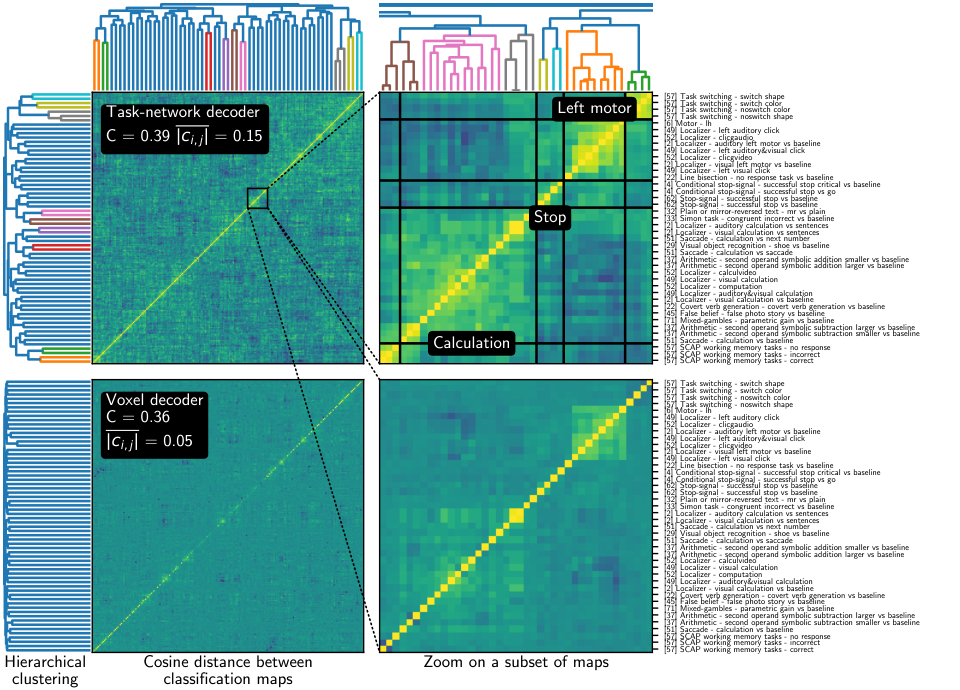
As our model is linear, we qualitatively compare the classification maps that it yields with maps obtained with a baseline single-study voxel-level decoding approach. For both approaches, we compute the correlation matrix between classification maps to uncover potential clusters of similar maps, using hierarchical clustering [61]. We compare this correlation matrix in term of how clustered it is, using the cophenetic correlation coefficient [62] and the mean absolute cosine similarity between maps.
Reusable tools and resources
Our approach can be used to improve statistical power of decoding in new fMRI studies. To facilitate its use, we have released resources and the cogspaces library (http://cogspaces.github.io). We include software to train the models. Pre-trained MSTONs networks (with associated word-clouds) can be downloaded and inspected on a dedicated page (https://cogspaces.github.io/assets/MSTON/components.html).The statistical maps used in the present study may be downloaded using our library, or on neurovault.org. The published MSTON networks hold the representations extracted from the 35 studies that we have considered; some of them are shown in Fig 4.
Results
We first detail the quantitative improvements brought by our approach, before exploring these results from a cognitive neuroscience point of view.
Improved statistical performance of multi-study decoding
Decoding from multi-study task optimized networks gives quantitative improvements in prediction of mental processes, as summarized in Fig 2. For 28 out of the 35 task-fMRI studies that we consider, the MSTON-based decoder outperforms single-study decoders (Fig 2A). It improves accuracy by 17% for the top studies, with a mean gain of 5.8% (80% experiments with net increase, 4.8% median gain) across studies and cross-validation splits (Fig 2B). Jointly minimizing errors on every study constructs second-layer representations that are efficient for many study-specific decoding tasks; the second layer parameters therefore incorporate information from all studies. This shared representation enables information transfer among the many decoding tasks performed by the third layer—predictive accuracy is thus improved thanks to transfer learning. Although we have not explicitly modeled how mental processes or psychological manipulations are related across experiments, our quantitative results show that these relations can be captured by the model—encoded into the second layer—to improve decoding performance.
Studies with diverse cognitive focus benefit from using multi-study modeling. The different decoding tasks have varying difficulties—we report performance sorted by chance level in Fig L, S1B Appendix.. Among the highest accuracy gains, we find cognitive control (stop-signal), classification studies, and localizer-like protocols. Our corpus contains many of such studies; as a result, multi-study decoding has access to many more samples to gather information on the associated cognitive networks. The activation of these networks is better captured in the shared part of the model, thereby leading to the observed improvement. In contrast, for a few studies, among which HCP and LA5C, we observe a slight negative transfer effect. This is not surprising—as HCP holds 900 subjects, it may not benefit from the aggregation of much smaller studies; LA5C focuses on higher-level cognitive processes with limited counterparts in the other studies, which precludes effective transfer.
Fig 2B shows that simply projecting data onto resting state functional networks instead of using our three-layer model does not significantly improve decoding, although the net accuracy gain varies from study to study. Adding a second task-optimized—supervised—dimension reduction is thus necessary to improve overall decoding accuracy. Functional contrasts that are either easy or very hard to decode do not benefit much from multi-study modeling, whereas classes with a balanced-accuracy around 80% experience the largest decoding improvement (Fig 2). We attribute this to two causes: easy-to-decode studies do not benefit from the extra signal provided by other studies, while some studies in our corpus are simply too hard to decode due to a low signal-to-noise ratio. Fig 2D shows that the benefit of multi-study modeling is higher for smaller studies, confirming that the proposed method boosts their inter-subject decoding performance.
In Fig 3, we vary the number of training subjects in target studies, and compare the performance of the multi-study decoder with a more standard one. We observe that the smaller the study size, the larger the performance gain brought by multi-study modeling. Transfer learning in inter-subject decoding is thus particularly effective for small studies (e.g., 16 subjects), that still constitute the essential of task-fMRI studies. To confirm this effect, we trained a multi-study model on a subset of subjects per study, considering studies that comprise more than subjects. In this case, the transfer learning effect is positive for all studies (Fig K in S1B Appendix.), including those for which negative transfer was observed when using full cohorts.
Finally, we show in Fig B (S1B Appendix.) that training a three-layer model and reusing the first two layers as a fixed dimension reduction when decoding a new study improves decoding accuracy on average. The extracted functional networks (MSTONs) thus provide a study-independent prior that is likely to improve decoding for studies probing different cognitive questions than the ones considered in the training corpus.

Multi-study task-optimized networks capture broad cognitive domains
We outline the contours of the 128 extracted MSTONs in Fig 4A. The networks almost cover the entire cortex, a consequence of the broad coverage of cognition of the studies we gathered. Task-optimized networks must indeed capture information to predict 545 different cognitive classes from the resulting distributed brain activity. Brain regions that are systematically recruited in task-fMRI protocols, e.g., motor cortex, auditory cortex, and primary visual cortex, are finely segmented by MSTON: they appear in several different networks. Capturing information in these regions is crucial for decoding many contrasts in our corpus, hence the model dedicates a large part of its representation capability to it. As decoding requires capturing distributed activations, MSTON are formed of multiple regions (Fig 4B). For instance, both parahippocampal gyri appear together in the yellow bottom-left network.
Most importantly, Fig 4B-C show that the model relates extracted MSTONs to specific cognitive information. The MSTONs each play a role in decoding a subset of contrasts. Components may capture low-level or high-level cognitive signal, though the low-level components are easier to interpret. Indeed, at a lower level, they outline the primary visual cortex, associated with contrasts such as checkerboard stimuli, and both hand motor cortices, associated with various tasks demanding motor functions. At a higher level, some interpretable components single out the left DLPFC and the IPS in separate networks, used to decode tasks related to calculation and comparison. Others delineate the language network and the right posterior insula, important in decoding tasks involving music [27]. Yet another MSTON delineates Broca’s area, associated with language tasks (Fig 5).
Inspecting the tasks associated with the MSTONs reveals structure-function links. Once again, the results are more interpretable for low-level functions, although some well-known high-level functional associations are also well captured. For instance, several components on Fig 4 involve brain regions recruited across a wide variety of tasks, such as the anterior insula, engaged in auditory and visual tasks [63] and considered to tackle ambiguous perceptual information, or the ACC, associated with tasks with affective components [64] and reward-based decision making [65]. Some MSTONs are more distributed, but correspond to well-known patterns brain activity. For example, Fig 5 show components that reveal parts the default mode networks –associated with baseline conditions, theory-of-mind tasks and prospection [66, 67]–, parts of the fronto-parietal control network –associated with a variety of problem-solving tasks [68]– and the dorsal attentional network –associated with visuo-spatial attention tasks such as saccades [69].
Visualizing MSTONs along with word-clouds serves essentially an illustratory purpose. It yields more interpretable results with focal networks than with distributed networks. In both cases, the words in the contrasts related to the given MSTONs capture documented structure-function associations. Interpretability may be improved by reducing the number of extracted networks, at the cost of a quantitative loss in performance. In particular, with components, the default mode network is split across several MSTONs (Fig 5). Such a splitting is common for high-dimensional decomposition of the fMRI signal, as noted in resting state [70], as a network such as the default-mode network has different sub-units with distinct functional contributions [71]. Conversely, some contrast maps are correlated with several distributed MSTONs, as illustrated in Fig A (S1B Appendix.).


Impact of multi-study modeling on classification maps
To better understand how multi-study training and layered representations improve decoding performance, we compare classification maps obtained using our model to standard decoder maps in Fig 6. For contrasts with significant accuracy gains, the classification maps are less noisy and more focal. They single out determinant regions more clearly, e.g., the fusiform face area (FFA, row 1) in classification maps for the face-vs-house contrast, or the left motor cortex in maps (row 2) predicting pumping action in BART tasks [29]. The language network is typically better delineated by our model (row 3), and so is the posterior insula in music-related contrasts (row 4). These improvements are due to two aspects: First, projecting onto a lower dimension subspace has a denoising effect on contrast maps, that is already at play when projecting onto simple resting-state functional networks. Second, multi-study training finds more scattered classification maps, as these combine complex MSTONs, learned on a large set of brain images. Our method slightly decreases performance for a small fraction of contrasts, such as maps associated with vertical checkerboard (row 5), a condition well localized and easy to decode from the original data. Our model renders them too much distributed, an unfortunate consequence of multi-study modeling.
We also compare original input contrast maps to their transformation by the projection on task-optimized networks (Fig C in S1B Appendix. ). Projected data are more focal, i.e. spatial variations that are unlikely to be related to cognition are smoothed. This offers a new angle on the quantitative results (Fig 2): brain activity expressed as the activation of these networks captures better cognition and allows decoders to generalize better across subjects than when classifying raw input directly.
Information transfer among classification maps.
In Fig 7, we compare the correlation between the 545 classification maps obtained using a multi-study decoder and using simple functional networks decoders. Classification maps learned using task-optimized networks are more correlated on average, and hierarchical clustering reveals a sharper correlation structure. This is because the whole classification matrix is low-rank (rank ) and influenced by the many studies we consider—the classification maps of our model are supported by networks relevant for cognition. As a consequence, it is easier to cluster maps into meaningful groups using hierarchical clustering based on cosine distances. For instance, we outline inter-study groups of maps related to left-motor functions, or calculation tasks. Hierarchical clustering on baseline maps is less successful: the associated dendrogram is less structured, and the distortion introduced by clusters is higher (as suggested by the smaller cophenetic coefficient). Clusters are harder to identify, due to smaller contrast in the correlation matrix. Multi-study training thus acts as a regularizer, by forcing correlation across maps with discovered relations. This regularization partly explains the increase in decoding accuracy.
Discussion
The methodology presented in this work harnesses the power of deep representations to build multi-study decoding models for brain functional images. It brings an immediate benefit to functional brain imaging by providing a universal way to improve the accuracy of decoding in a newly acquired dataset. Decoding is a central tool to draw inferences on which brain structures implement the neural support of the observed behavior. It is most often applied to task-fMRI studies with 30 or less subjects, which tend to lack statistical power [72]. In this regime, aggregating existing studies to a new one using a multi-study model as the one we propose is likely to improve decoding performance. This is further evidenced in Fig B (S1B Appendix.): using MSTONs as a decoding basis on a new decoding task outperforms using resting-state networks. Of course, such improvement can only occur if the cognitive functions probed by the new study are related to the ones probed in the multi-study corpus. We foresee limited benefits when analyzing strongly original task fMRI experiments, and experiments studying very specific and high-level cognitive functions, that MSTONs are only partially able to capture (Fig 5).
With increasing availability of shared and normalized data, multi-study modeling is an important improvement over simple decoders, provided that it can adapt to the diversity of cognitive paradigms. Our transfer-learning model has such flexibility, as it does not require explicit correspondence across experiments. Beyond quantitative benefits –the gain in prediction accuracy– the models also brings qualitative benefits, facilitating the interpretation of decoding maps (Fig 6). Pooling subjects across studies effectively increases the sample size, as advocated by [2]. The resulting increase in statistical power for cognitive modeling will help addressing the reproducibility challenge outlined by [3]. In our setting, each study (or site) provides a single decoding objective, which is predicting one contrast among all other contrasts from this study. This is a validated approach in decoding [73]. As some studies use different fMRI tasks, we may also use one decoding objective per task, with similar quantitative improvement in performance (see Fig F in S1B Appendix.).
Our modeling choices were driven by the recent successes of deep non-linear models in computer vision and medical imaging. However, we were not able to increase performance by departing from linear models: introducing non linearities in our models provides no improvement on left-out accuracy. On the other hand, we have shown that pooling many fMRI data sources enables to learn deeper models, although these remain linear. Techniques developed in deep learning prove useful to fit models that generalize well across subjects: using dropout regularization [14] and advanced stochastic gradient techniques [13] is crucial for successful transfer and good generalization performance.
Sticking to linear models brings the benefit of easy interpretation of decoding models. The use of sparsity and non-negativity in the training and consensus phase allow to obtain interpretable networks. Using sparsity only in each phase (as originally advocated by [74]) yields “contrast” networks with both positive and negative regions, that are harder to interpret (see also [60]). In particular, this limits the occurence of non-zero weights that reflect noise suppression [75].
The models capture information relevant for many decoding tasks in their internal representations. From these internals, we extract interpretable cognitive networks, inspired by matrix factorization techniques used to interpret computer vision models [76]. The good predictive performance of MSTONs networks (Fig 2 and Fig B in S1B Appendix.) provides quantitative support for their decomposition of brain function. Extracting a universal basis of cognition is beyond the scope of a single fMRI study, and should be done by analysis across many studies. We show that, across studies, a joint predictive model finds meaningful approximations of atomic cognitive functions spanning a wide variety of mental processes (Fig 4). This methodology provides a step forward towards defining mental processes in a quantitative manner, which remains a fundamental challenge in psychology [77, 9]. Yet, in the present work, the delineation of atomic cognitive functions remains coarse and incomplete. This is likely due to the limited scope of our corpus, and to the fact that we automatically align the cognitive functions probed by the various studies of the corpus. Expert annotation of mental process involved in the studies could greatly help establishing a clearer picture.
Our approach differs from commonly-used decomposition techniques in fMRI analysis (e.g. ICA [78], or dictionary learning [74]), that are used to extract functional networks. These techniques optimize an unsupervised reconstruction objective over resting-state data, in effect capturing co-occurrence of brain activity across distributed locations. They have traditionally been used with few components (e.g. ). In contrast, after the first decomposition, performed without information from the tasks, we extract the MSTONs components to optimize the decoding performance on many tasks. Leaving a systematic comparison between MSTONs and classical functional networks for future work, we already make two observations. First, a fraction of functional networks extracted by unsupervised methods support non-Gaussian noise patterns in the BOLD time-series, and permits noise suppression [79, 80]. Typically, only a fraction of the networks extracted in an ICA analysis is interpreted. MSTONs, on the other hand, optimize a supervised objective and focus on the fraction of the BOLD signal related to the tasks. Second, MSTONs (despite being more noisy) appears more skewed towards known coordinated brain networks (Figs 4 and 5), that differs from the networks recruited at rest (see e.g. [81] for a comparison of task and rest brain networks).
We use many different fMRI studies to distill MSTONs across various tasks. This data aggregation approach requires little supervison. The flip side is that it leads to coarse results by nature: our approach is obviously not sufficient to recover the detailed brain-to-mind mapping, collective knowledge of psychologists and neuroscientists, that has emerged from decades of research on multimodal datasets and careful behavioral experiments. Specific brain-to-mind associations are best resolved with dedicated experiments using experimental-pyschology paradigms tailored to the question at hand. Other data than fMRI, for instance more invasive, may also provide stronger evidence. For instance a double dissociation in brain-lesion patients give unambiguous evidence of distinct cognitive processes via distant neural supports, as with Broca and Wernicke’s separation of language understanding and generation [82], or the more recent teasing out of emotional and cognitive empathy [83].
Finally, the current version of our framework does not model explicit inter-subject variability, and is rather focused on extracting commonalities across subjects. Future work may augment multi-study decoding with such information, as obtained by e.g., hyperalignment techniques [84].
Conclusion
The success of using distributed representations to bridge cognitive tasks supports a system-level view on how brain activity supports cognition.
Our multi-study model will become increasingly useful to brain imaging as the number of available studies grows. Such a growth is driven by the steady increase of publicly shared brain-imaging data, facilitated by online neuroimaging platforms and increased standardization [85, 2]. With a larger corpus of studies, the proposed methodology has the potential to build even better universal priors that overall improve statistical power for functional brain imaging. As such, multi-study decoding provides a path towards knowledge consolidation in functional neuroimaging and cognitive neuroscience.
References
- 1. Yarkoni T, Poldrack RA, Nichols TE, Van Essen DC, Wager TD. Large-Scale Automated Synthesis of Human Functional Neuroimaging Data. Nature Methods. 2011;8(8):665–670.
- 2. Poldrack RA, Baker CI, Durnez J, Gorgolewski KJ, Matthews PM, Munafò MR, et al. Scanning the Horizon: Towards Transparent and Reproducible Neuroimaging Research. Nature Reviews Neuroscience. 2017;18(2):115–126.
- 3. Button KS, Ioannidis JPA, Mokrysz C, Nosek BA, Flint J, Robinson ESJ, et al. Power Failure: Why Small Sample Size Undermines the Reliability of Neuroscience. Nature Reviews Neuroscience. 2013;14(5):365–376.
- 4. Van Essen DC, Ugurbil K, Auerbach E, Barch D, Behrens TEJ, Bucholz R, et al. The Human Connectome Project: A Data Acquisition Perspective. NeuroImage. 2012;62(4):2222–2231.
- 5. Miller KL, Alfaro-Almagro F, Bangerter NK, Thomas DL, Yacoub E, Xu J, et al. Multimodal Population Brain Imaging in the UK Biobank Prospective Epidemiological Study. Nature Neuroscience. 2016;19(11):1523–1536.
- 6. Poldrack RA. Can cognitive processes be inferred from neuroimaging data? Trends in cognitive sciences. 2006;10(2):59–63.
- 7. Haxby JV, Gobbini IM, Furey ML, Ishai A, Schouten JL, Pietrini P. Distributed and Overlapping Representations of Faces and Objects in Ventral Temporal Cortex. Science. 2001;293(5539):2425–2430.
- 8. Poldrack RA, Halchenko YO, Hanson SJ. Decoding the Large-Scale Structure of Brain Function by Classifying Mental States Across Individuals. Psychological Science. 2009;20(11):1364–1372.
- 9. Poldrack RA, Barch DM, Mitchell J, Wager TD, Wagner AD, Devlin JT, et al. Toward Open Sharing of Task-Based fMRI Data: The OpenfMRI Project. Frontiers in Neuroinformatics. 2013;7:12.
- 10. Gorgolewski KJ, Varoquaux G, Rivera G, Schwarz Y, Ghosh SS, Maumet C, et al. NeuroVault.org: A Web-Based Repository for Collecting and Sharing Unthresholded Statistical Maps of the Human Brain. Frontiers in Neuroinformatics. 2015;9:8.
- 11. Ando RK, Zhang T. A Framework for Learning Predictive Structures from Multiple Tasks and Unlabeled Data. Journal of Machine Learning Research. 2005;6:1817–1853.
- 12. Xue Y, Liao X, Carin L, Krishnapuram B. Multi-Task Learning for Classification with Dirichlet Process Priors. Journal of Machine Learning Research. 2007;8(Jan):35–63.
- 13. Kingma DP, Ba J. Adam: A Method for Stochastic Optimization. In: International Conference for Learning Representations; 2015.
- 14. Srivastava N, Hinton GE, Krizhevsky A, Sutskever I, Salakhutdinov R. Dropout: A Simple Way to Prevent Neural Networks from Overfitting. Journal of Machine Learning Research. 2014;15(1):1929–1958.
- 15. Varoquaux G, Poldrack RA. Predictive models avoid excessive reductionism in cognitive neuroimaging. Current opinion in neurobiology. 2019;55:1–6.
- 16. Newell A. You Can’t Play 20 Questions with Nature and Win: Projective Comments on the Papers of This Symposium. Visual Information Processing. 1973; p. 1–26.
- 17. Wager TD, Atlas LY, Lindquist MA, Roy M, Woo CW, Kross E. An fMRI-Based Neurologic Signature of Physical Pain. New England Journal of Medicine. 2013;368(15):1388–1397.
- 18. Varoquaux G, Schwartz Y, Poldrack RA, Gauthier B, Bzdok D, Poline JB, et al. Atlases of cognition with large-scale human brain mapping. PLoS computational biology. 2018;14(11):e1006565.
- 19. Poldrack RA, Yarkoni T. From Brain Maps to Cognitive Ontologies: Informatics and the Search for Mental Structure. Annual Review of Psychology. 2016;67(1):587–612.
- 20. Barrett LF. The Future of Psychology: Connecting Mind to Brain. Perspectives on Psychological Science. 2009;4(4):326–339.
- 21. Mensch A, Mairal J, Bzdok D, Thirion B, Varoquaux G. Learning Neural Representations of Human Cognition Across Many fMRI Studies. In: Advances in Neural Information Processing Systems; 2017. p. 5883–5893.
- 22. Amalric M, Dehaene S. Origins of the Brain Networks for Advanced Mathematics in Expert Mathematicians. Proceedings of the National Academy of Sciences. 2016;113(18):4909–4917.
- 23. Pinel P, Thirion B, Meriaux S, Jobert A, Serres J, Bihan DL, et al. Fast Reproducible Identification and Large-Scale Databasing of Individual Functional Cognitive Networks. BMC neuroscience. 2007;8:91.
- 24. Papadopoulos Orfanos D, Michel V, Schwartz Y, Pinel P, Moreno A, Le Bihan D, et al. The Brainomics/Localizer Database. NeuroImage. 2017;144:309–314.
- 25. Shafto MA, Tyler LK, Dixon M, Taylor JR, Rowe JB, Cusack R, et al. The Cambridge Centre for Ageing and Neuroscience (Cam-CAN) Study Protocol: A Cross-Sectional, Lifespan, Multidisciplinary Examination of Healthy Cognitive Ageing. BMC Neurology. 2014;14:204.
- 26. Cauvet E. Traitement des structures syntaxiques dans le langage et dans la musique [PhD thesis]. Paris 6; 2012.
- 27. Hara N, Cauvet E, Devauchelle AD, Dehaene S, Pallier C, et al. Neural Correlates of Constituent Structure in Language and Music. NeuroImage. 2009;47:S143.
- 28. Devauchelle AD, Oppenheim C, Rizzi L, Dehaene S, Pallier C. Sentence Syntax and Content in the Human Temporal Lobe: An fMRI Adaptation Study in Auditory and Visual Modalities. Journal of Cognitive Neuroscience. 2009;21(5):1000–1012.
- 29. Schonberg T, Fox C, Mumford JA, Congdon C, Trepel C, Poldrack RA. Decreasing Ventromedial Prefrontal Cortex Activity During Sequential Risk-Taking: An fMRI Investigation of the Balloon Analog Risk Task. Frontiers in Neuroscience. 2012;6:80.
- 30. Aron AR, Gluck M, Poldrack RA. Long-Term Test–Retest Reliability of Functional MRI in a Classification Learning Task. NeuroImage. 2006;29:1000–1006.
- 31. Xue G, Poldrack RA. The Neural Substrates of Visual Perceptual Learning of Words: Implications for the Visual Word Form Area Hypothesis. Journal of Cognitive Neuroscience. 2007;19:1643–1655.
- 32. Tom SM, Fox CR, Trepel C, Poldrack RA. The Neural Basis of Loss Aversion in Decision-Making Under Risk. Science. 2007;315(5811):515–518.
- 33. Jimura K, Cazalis F, Stover ERS, Poldrack RA. The Neural Basis of Task Switching Changes with Skill Acquisition. Frontiers in Human Neuroscience. 2014;8.
- 34. Xue G, Aron AR, Poldrack RA. Common Neural Substrates for Inhibition of Spoken and Manual Responses. Cerebral Cortex. 2008;18:1923–1932.
- 35. Aron AR, Behrens TE, Smith S, Frank MJ, Poldrack RA. Triangulating a Cognitive Control Network Using Diffusion-Weighted Magnetic Resonance Imaging (MRI) and Functional MRI. The Journal of Neuroscience. 2007;27:3743–3752.
- 36. Cohen JR. The Development and Generality of Self-Control [PhD thesis]. University of the City of Los Angeles; 2009.
- 37. Foerde K, Knowlton B, Poldrack RA. Modulation of Competing Memory Systems by Distraction. Proceedings of the National Academy of Science. 2006;103:11778–11783.
- 38. Rizk-Jackson A, Aron AR, Poldrack RA. Classification Learning and Stop-Signal (one Year Test-Retest); 2011. https://openfmri.org/dataset/ds000017.
- 39. Alvarez RP, Jasdzewski G, Poldrack RA. Building Memories in Two Languages: An fMRI Study of Episodic Encoding in Bilinguals. In: Society for Neuroscience Abstracts; 2002. p. 179.12.
- 40. Poldrack RA, Clark J, Pare-Blagoev E, Shohamy D, Creso Moyano J, Myers C, et al. Interactive Memory Systems in the Human Brain. Nature. 2001;414(6863):546–550.
- 41. Kelly A, Milham M. Simon Task; 2011. https://openfmri.org/dataset/ds000101.
- 42. Duncan K, Pattamadilok C, Knierim I, Devlin J. Consistency and Variability in Functional Localisers. NeuroImage. 2009;46:1018–1026.
- 43. Wager TD, Davidson ML, Hughes BL, Lindquist MA, Ochsner KN. Prefrontal-Subcortical Pathways Mediating Successful Emotion Regulation. Neuron. 2008;59:1037–1050.
- 44. Moran JM, Jolly E, Mitchell JP. Social-Cognitive Deficits in Normal Aging. The Journal of Neuroscience. 2012;32:5553–5561.
- 45. Uncapher MR, Hutchinson JB, Wagner AD. Dissociable Effects of Top-Down and Bottom-Up Attention During Episodic Encoding. The Journal of Neuroscience: The Official Journal of the Society for Neuroscience. 2011;31(35):12613–12628.
- 46. Gorgolewski KJ, Storkey A, Bastin ME, Whittle IR, Wardlaw JM, Pernet CR. A Test-Retest fMRI Dataset for Motor, Language and Spatial Attention Functions. GigaScience. 2013;2(1):6.
- 47. Collier AK, Wolf DH, Valdez JN, Turetsky BI, Elliott MA, Gur RE, et al. Comparison of Auditory and Visual Oddball fMRI in Schizophrenia. Schizophrenia research. 2014;158:183–188.
- 48. Gauthier B, Eger E, Hesselmann G, Giraud AL, Kleinschmidt A. Temporal Tuning Properties Along the Human Ventral Visual Stream. The Journal of Neuroscience. 2012;32:14433–14441.
- 49. Barch DM, Burgess GC, Harms MP, Petersen SE, Schlaggar BL, Corbetta M, et al. Function in the Human Connectome: Task-fMRI and Individual Differences in Behavior. NeuroImage. 2013;80:169–189.
- 50. Henson RN, Wakeman DG, Litvak V, Friston KJ. A Parametric Empirical Bayesian Framework for the EEG/MEG Inverse Problem: Generative Models for Multi-Subject and Multi-Modal Integration. Frontiers in Human Neuroscience. 2011;5.
- 51. Knops A, Thirion B, Hubbard EM, Michel V, Dehaene S. Recruitment of an Area Involved in Eye Movements During Mental Arithmetic. Science. 2009;324:1583–1585.
- 52. Poldrack RA, Congdon E, Triplett W, Gorgolewski KJ, Karlsgodt K, Mumford JA, et al. A Phenome-Wide Examination of Neural and Cognitive Function. Scientific Data. 2016;3:160110.
- 53. Pinel P, Dehaene S. Genetic and Environmental Contributions to Brain Activation During Calculation. NeuroImage. 2013;81:306–316.
- 54. Vagharchakian L, Dehaene-Lambertz G, Pallier C, Dehaene S. A Temporal Bottleneck in the Language Comprehension Network. The Journal of Neuroscience. 2012;32:9089–9102.
- 55. Pan SJ, Yang Q. A Survey on Transfer Learning. IEEE Transactions on Knowledge and Data Engineering. 2010;22(10):1345–1359.
- 56. Kingma DP, Salimans T, Welling M. Variational Dropout and the Local Reparameterization Trick. In: Advances in Neural Information Processing Systems; 2015. p. 2575–2583.
- 57. Friston KJ, Holmes AP, Worsley KJ, Poline JP, Frith CD, Frackowiak RS. Statistical Parametric Maps in Functional Imaging: A General Linear Approach. Human brain mapping. 1994;2(4):189–210.
- 58. Mairal J, Bach F, Ponce J, Sapiro G. Online Learning for Matrix Factorization and Sparse Coding. Journal of Machine Learning Research. 2010;11:19–60.
- 59. Mensch A, Mairal J, Thirion B, Varoquaux G. Stochastic Subsampling for Factorizing Huge Matrices. IEEE Transactions on Signal Processing. 2018;66(1):113–128.
- 60. Dadi K, Varoquaux G, Machlouzarides-Shalit A, Gorgolewski KJ, Wassermann D, Thirion B, et al. Fine-grain atlases of functional modes for fMRI analysis. To appear in NeuroImage. 2020;.
- 61. Gower JC, Ross GJ. Minimum Spanning Trees and Single Linkage Cluster Analysis. Journal of the Royal Statistical Society: Series C (Applied Statistics);18(1):54–64.
- 62. Sokal RR, Rohlf FJ. The Comparison of Dendrograms by Objective Methods. Taxon; p. 33–40.
- 63. Braver TS, Barch DM, Gray JR, Molfese DL, Snyder A. Anterior cingulate cortex and response conflict: effects of frequency, inhibition and errors. Cerebral cortex. 2001;11:825.
- 64. Stevens FL, Hurley RA, Taber KH. Anterior cingulate cortex: unique role in cognition and emotion. The Journal of neuropsychiatry and clinical neurosciences. 2011;23(2):121.
- 65. Bush G, Vogt BA, Holmes J, Dale AM, Greve D, Jenike MA, et al. Dorsal anterior cingulate cortex: a role in reward-based decision making. Proceedings of the National Academy of Sciences. 2002;99:523–528.
- 66. Raichle ME, MacLeod AM, Snyder AZ, Powers WJ, Gusnard DA, Shulman GL. A default mode of brain function. Proceedings of the National Academy of Sciences. 2001;98(2):676–682.
- 67. Spreng RN, Grady CL. Patterns of brain activity supporting autobiographical memory, prospection, and theory of mind, and their relationship to the default mode network. Journal of cognitive neuroscience. 2010;22:1112.
- 68. Gratton C, Sun H, Petersen SE. Control networks and hubs. Psychophysiology. 2018;55:e13032.
- 69. Ptak R. The frontoparietal attention network of the human brain: action, saliency, and a priority map of the environment. The Neuroscientist. 2012;18(5):502–515.
- 70. Kiviniemi V, Starck T, Remes J, Long X, Nikkinen J, Haapea M, et al. Functional segmentation of the brain cortex using high model order group PICA. Human brain mapping. 2009;30(12):3865–3886.
- 71. Leech R, Kamourieh S, Beckmann CF, Sharp DJ. Fractionating the default mode network: distinct contributions of the ventral and dorsal posterior cingulate cortex to cognitive control. Journal of Neuroscience. 2011;31(9):3217–3224.
- 72. Varoquaux G. Cross-Validation Failure: Small Sample Sizes Lead to Large Error Bars. NeuroImage. 2018;180:68–77.
- 73. Bzdok D, Eickenberg M, Grisel O, Thirion B, Varoquaux G. Semi-Supervised Factored Logistic Regression for High-Dimensional Neuroimaging Data. In: Advances in Neural Information Processing Systems; 2015. p. 3348–3356.
- 74. Varoquaux G, Gramfort A, Pedregosa F, Michel V, Thirion B. Multi-Subject Dictionary Learning to Segment an Atlas of Brain Spontaneous Activity. Proceedings of the International Conference on Information Processing in Medical Imaging. 2011;22:562.
- 75. Haufe S, Meinecke F, Görgen K, Dähne S, Haynes JD, Blankertz B, et al. On the Interpretation of Weight Vectors of Linear Models in Multivariate Neuroimaging. NeuroImage;87:96–110.
- 76. Olah C, Satyanarayan A, Johnson I, Carter S, Schubert L, Ye K, et al. The Building Blocks of Interpretability. Distill. 2018;3(3):e10.
- 77. Uttal WR. The New Phrenology: The Limits of Localizing Cognitive Processes in the Brain. The MIT press; 2001.
- 78. McKeown MJ, Makeig S, Brown GG, Jung TP, Kindermann SS, Bell AJ, et al. Analysis of fMRI Data by Blind Separation Into Independent Spatial Components. Human Brain Mapping. 1998;6(3):160–188.
- 79. Perlbarg V, Bellec P, Anton JL, Pélégrini-Issac M, Doyon J, Benali H. CORSICA: correction of structured noise in fMRI by automatic identification of ICA components. Magnetic resonance imaging. 2007;25(1):35–46.
- 80. Salimi-Khorshidi G, Douaud G, Beckmann CF, Glasser MF, Griffanti L, Smith SM. Automatic denoising of functional MRI data: combining independent component analysis and hierarchical fusion of classifiers. Neuroimage. 2014;90:449–468.
- 81. Laird AR, Fox PM, Eickhoff SB, Turner JA, Ray KL, McKay DR, et al. Behavioral interpretations of intrinsic connectivity networks. Journal of cognitive neuroscience. 2011;23(12):4022–4037.
- 82. Friederici AD, Hahne A, Von Cramon DY. First-pass versus second-pass parsing processes in a Wernicke’s and a Broca’s aphasic: electrophysiological evidence for a double dissociation. Brain and language. 1998;62:311.
- 83. Shamay-Tsoory SG, Aharon-Peretz J, Perry D. Two systems for empathy: a double dissociation between emotional and cognitive empathy in inferior frontal gyrus versus ventromedial prefrontal lesions. Brain. 2009;132:617.
- 84. Haxby JV, Guntupalli JS, Connolly AC, Halchenko YO, Conroy BR, Gobbini MI, et al. A Common, High-Dimensional Model of the Representational Space in Human Ventral Temporal Cortex. Neuron. 2011;72(2):404–416.
- 85. Gorgolewski KJ, Auer T, Calhoun VD, Craddock RC, Das S, Duff EP, et al. The Brain Imaging Data Structure, a Format for Organizing and Describing Outputs of Neuroimaging Experiments. Scientific Data. 2016;3:sdata201644.
- 86. Smith SM, Fox PT, Miller KL, Glahn DC, Fox PM, Mackay CE, et al. Correspondence of the Brain’s Functional Architecture During Activation and Rest. Proceedings of the National Academy of Sciences. 2009;106(31):13040–13045.
- 87. Yeo TBT, Krienen FM, Sepulcre J, Sabuncu MR, Lashkari D, Hollinshead M, et al. The Organization of the Human Cerebral Cortex Estimated by Intrinsic Functional Connectivity. Journal of Neurophysiology. 2011;106(3):1125–1165.
- 88. Nocedal J. Updating Quasi-Newton Matrices with Limited Storage. Mathematics of Computation. 1980;35(151):773–782.
- 89. Neyshabur B. Implicit Regularization in Deep Learning [PhD thesis]. Toyota Technological Institute at Chicago; 2017.
- 90. Molchanov D, Ashukha A, Vetrov D. Variational Dropout Sparsifies Deep Neural Networks. In: Proceedings of the International Conference on Machine Learning; 2017. p. 2498–2507.
- 91. Ioffe S, Szegedy C. Batch Normalization: Accelerating Deep Network Training by Reducing Internal Covariate Shift. In: Proceedings of the International Conference on Machine Learning; 2015. p. 448–456.
- 92. Srebro N, Rennie J, Jaakkola TS. Maximum-Margin Matrix Factorization. In: Advances in Neural Information Processing Systems; 2004. p. 1329–1336.
- 93. Beck A, Teboulle M. A Fast Iterative Shrinkage-Thresholding Algorithm for Linear Inverse Problems. SIAM Journal on Imaging Sciences. 2009;2(1):183–202.
- 94. Rennie JDM, Srebro N. Fast Maximum Margin Matrix Factorization for Collaborative Prediction. In: Proceedings of the International Conference on Machine Learning; 2005. p. 713–719.
- 95. Bell RM, Koren Y. Lessons from the Netflix Prize Challenge. ACM SIGKDD Explorations Newsletter. 2007;9(2):75–79.
- 96. Wager S, Wang S, Liang PS. Dropout Training as Adaptive Regularization. In: Advances in Neural Information Processing Systems; 2013. p. 351–359.
- 97. Breiman L. Bagging Predictors. Machine Learning. 1996;24(2):123–140.
- 98. Abraham A, Pedregosa F, Eickenberg M, Gervais P, Mueller A, Kossaifi J, et al. Machine Learning for Neuroimaging with Scikit-Learn. Frontiers in Neuroinformatics. 2014;8:14.
- 99. Pedregosa F, Varoquaux G, Gramfort A, Michel V, Thirion B, Grisel O, et al. Scikit-Learn: Machine Learning in Python. Journal of Machine Learning Research. 2011;12:2825–2830.
- 100. Paszke A, Gross S, Chintala S, Chanan G. PyTorch: Tensors and Dynamic Neural Networks in Python with Strong GPU Acceleration; 2017.
Supporting information
S1A Appendix.
Detailed methods. This appendix discusses technical details of the multi-study decoding approach: the specific architecture, a 3-layer linear model, and the deep-learning technique used to regularize and train it.
S1B Appendix.
Discussion on the model design. In this appendix, we perform supportive experiments to explain the observed results, An ablation study of the various model components is provided to further support modelling choices.
S1C Appendix.
Reproduction details and tables. In this appendix, we provide implementation details for reproducibility, along with tables with quantitative results per contrast.
S1 Appendix
The appendix is structured as follow: in the first section, we formalize the learning setting and method, after describing decoding baselines. In the second section, we perform supportive experiments to explain the observed results, and discuss various alternatives for the model, to further support modelling choices. Finally, we provide reproduction details, along with data and software notes. A visualization of all MSTONs components (that reproduces https://cogspaces.github.io/assets/MSTON/components.html) is provided for completeness in S1 Components.
Notations.
We denote scalars, vectors and matrices using lower-case, bold lower-case and bold upper-case letters, e.g., , and . We denote the elements of by and its rows by . We write a value that is specific to study number . We denote a value built from an ensemble of value . Finally, we write the set of integers ranging from to .
Appendix A Methods
We describe in mathematical terms the multi-layer decoder at the center of our method and provide supporting experiments. We start by formalizing the joint objective loss and the model training process.
A.1 Inter-subject decoding setting
We consider task functional MRI studies (detailed in Table 1), on which we perform inter-subject decoding. In study number , subjects are made to perform one (or sometimes several) tasks. Acquired BOLD time-series are registered to a common template using non-linear spatial registration, after motion and slice-timing corrections. BOLD time-series are then fed to a standard analysis pipeline, which fits a linear model relating the design matrix of each experiment to the signal in every voxel. We use the nistats library for this purpose. From the obtained beta maps, we compute z-statistics maps, either associated with each of the base conditions (stimulus or task) of the experiments, or with contrasts defined by the study’s authors. In both cases, z-maps are labeled with a number that corresponds to -th contrast/base condition (called contrast in the following). Overall, this produces a set of z-maps living in , where is the number of voxels, associated with a sequence of contrast . The transformation from 3D brain images to 1D vectors is done using a grey-matter mask after alignment with the MNI template. We compare using a grey-matter mask with using a full brain mask in Section B.4.1. Inter-subject decoding proposes a model that predicts contrast identity from z-maps, i.e., , where is learned from training data, and the performance of the model is assessed on left-out subjects.
A.2 Baseline voxel-space decoder
Baseline decoders are linear classifier models defined separately for each study , which take full brain images as input. For every input map in , we compute the logits in as
| (3) |
where and are the parameters of the linear model to be learned for study —we drop the superscript in this paragraph and the next for simplicity. Logits are transformed into a classification probability vector using the softmax operator. At test time, we predict the label corresponding to the maximal logit, i.e., . The model is trained on the data by minimizing the regularized multinomial classification problem
| (4) | ||||
| (5) |
where is the Frobenius norm, that computes .
A.3 Baseline dimension reduced decoder
A variant of the voxel-based decoders is obtained by introducing a first-layer dimension reduction learned from resting-state data. This amounts to computing
| (6) |
where in forms the classifying weights of the model, and the matrix in is assigned during training to functional networks learned on resting-state data, as detailed in A.5. Multiplying input data by projects statistical images onto meaningful resting-state components, in an attempt to improve classification performance and reduce computation cost, akin to the methods proposed by [86, 87]. The model is trained by solving the convex objective (5) separately for each study, replacing by in :
| (7) | ||||
| (8) |
Our results (Fig 2C) show that decoding from functional networks is not significantly better than decoding from voxels directly. For both baselines, the parameter is found by half-split cross-validation. Training is performed using a L-BFGS solver [88]. We use non standardized maps as input as we observed that standardization hinders performance.
A.4 Three-layer model description
Our three-layer model adds a second shared linear layer in between the projection on functional networks and the classification models. We still have
| (9) |
for every z-map and study . However, we introduce a coupling between the various parameters of each study: they should decompose on common basis , where is estimated from the whole corpus of data, and is the resting-state dictionary presented above. Formally, we assume that there exist a matrix in with , and a set of matrices so that for all , the classification weights of (5) writes
| (10) |
The matrix corresponds to the first-layer weights pictured in Fig 1, to the second-layer weights, and to the various classification heads of the third layer. In this work, we choose and . While remains fixed, the second-layer matrix and the classification heads are jointly learned during training, a necessary step toward improving decoding accuracy. The “shared-layer” parameterization (10) is a common approach in multi-task learning [11, 12], and should allow transfer learning between decoding tasks, under certain conditions. In our setting, both the data distribution from the different studies and the classification task associated with each study differ—this is a particular case of inductive transfer learning11 1 This case is less studied than the classical multi-task setting where input data are single-source but learning tasks are multiple., described by [55].
Modeling.
Without refinement nor regularization, we seek a local minimizer of the following non-convex objective function, which combines the classification objectives (5) from all studies, with parameter sharing:
| (11) | ||||
| (12) |
where the dependence on is left implicit. The scalar in is a parameter that regulates the importance of each study in the joint objective, that we further discuss in B.8. We note that the importance of the study to find the latent parameter depends on the amplitude of the gradient that does not depend on the number of tasks : in particular, for each study , contrast and subject , the susceptibility of the loss to the logits is such that , independent from .
Regularization.
We observe that minimizing (11) leads to strong overfitting and low performance on left-out data, with performance similar to fitting (5) without regularization, separately for each study. Adding regularization to the second and third layer weights gives little benefit, as we discuss in Section B.2.3. On the other hand, introducing dropout [14] during training alleviates the overfitting issue and fosters transfer learning. Dropout is a stochastic regularization method that prevents the weights from each layer to co-adapt by perturbating them with multiplicative noise during training. It ensures that the information is well spread across coefficients rows and columns [89]. In our case, this favors transfer learning, as it ensures that no single row of , or in plain words no task-optimized network, becomes dedicated to a single study. We further compare the different methods that we can use to foster transfer of information between studies in Section B.2.
We use the variational flavor of dropout [56] to make the dropout rate for every study adaptive. This slightly improves performance compared to binary dropout: every decoding task requires a different level of regularization, depending on the size of the study and the hardness of the task, and it is beneficial to estimate it from data. In details, during training, at every iteration, for every input sample of a mini-batch from study , we randomly draw two multiplicative noise matrices
| (13) |
where and , with fixed and estimated from data.22 2 This Gaussian dropout has a similar behavior to the more commonly used binary dropout with parameter . We then compute the noisy logits
| (14) |
and use these to compute the loss (15), to which we add a regularization term that regulates the learning of , introduced by [90]. We compute the gradient with respect to , , using the local reparametrization trick [56]. We refer to [90] for more details on variational dropout and a Bayesian grounding of this approach.
Optimization.
We solve the problem (11) using stochastic optimization. Namely, at each iteration, we compute an unbiased estimate of the objective (11) and its gradient with respect to the model parameters, in order to perform a stochastic gradient step. For this, we randomly choose the study with a probability proportional to , and consider a mini-batch of z-maps that we use to compute the unbiased objective estimate
| (15) |
from which we compute gradients with respect to , and .
A.5 Resting-state data
As mentioned above, we use resting-state data to compute the first-layer weights in , where . Such high-order dictionaries are known to perform well for decoding [60]. We consider data from the HCP900 release, and stack all records to obtain a data matrix in . We then use an online solver [59] to solve the sparse non-negative matrix factorization problem
| (16) |
where the constraint enforces every dictionary component to live in the simplex of , ensuring sparsity and non-negativity of the functional networks. The sparsity level is chosen so that the functional networks cover the whole brain with as little overlap as possible. Larger overlap leads to more correlated activations input to the second layer, yielding a harder learning problem. With lower coverage, we would miss important information to decode some of the predicted psychological conditions. We refer to [60] for further discussion on selecting sparsity level when using dictionary learning in fMRI analysis.
Second-layer initialization.
To initialize the weights of the second layer, we learn a smaller dictionary in as in (16), where . We then compute the initial weights so that using least-square regression. This way, applying the first two layers initially amount to projecting data onto larger functional networks , which is a reasonable prior for reducing the dimension of brain statistical maps. Using this resting-state based initialization slightly improves performance, as we discuss in Section B.4.
Grey matter restriction.
To help interpreting the obtained model, we found it helpful to remove from the fraction (9%) of the functional networks components located in the white matter and the cerebrospinal fluid areas, turning into . We discuss the effect of this restriction in Section B.4.1.
A.6 Model introspection with ensembling
Given any invertible matrix in , the non regularized version of the objective (11) is left invariant when transforming into and each into . This prevents us from interpreting the coefficients of at the end of the training procedure, and to retrieve relevant networks by reading the weights of the second weight. The only aspect of that remains unchanged after a linear parameter transformation is its span. Dropout regularization, which favors the canonical directions in matrix space [14], should break this symmetry, but does not help to uncover meaningful directions in the span of in practice.
On the other hand, we found that this span was remarkably stable across runs on the same data, whether when varying initialization or simply the order in which data are streamed during stochastic gradient descent. More precisely, we trained our model 100 times with different seeds, and concatenated the weights of the second-layer into a big matrix . We performed a SVD on this matrix, and observed that the first components captured 98% of the variance of when using the same initialization but different streaming order, and 96% when also using a different random initialization. Despite the many local minima that objective (11) admits, the span of thus remains close to some reference span that we can extract with a matrix factorization method.
The above remark suggested the following ensemble method. We run the learning algorithm times, and store the weights of the second layer for each run, along with the average matrices and biases
| (17) |
that combine the second and third-layer weights and biases for each study and run , and average them across runs. We then stack the second-layer weights into a tall matrix on which we perform sparse non-negative matrix factorization. Namely, we compute , the new weight matrix for the second layer, solving
| (18) |
where and regulates the sparsity of —performance little depends on provided it leads to finding with more than 50% non-zero voxels (see Section C.1). Higher leads to sparser maps with lower performance as brain coverage is reduced, while lower gives good performances but lower interpretability of the extracted networks. Finally, we compute new weights for all the classification heads of the third layer, so that , from a least-square point of view, for each study . The new model is then formed of parameters . In plain words, we obtain sparse non-negative second-layer weights , and define from these weights a new model that is as close as possible to the ensemble of all learned models .
The rows of are now interpretable separately, as the non-negative and sparse constraints have broken the inherent parameter invariance of the original model. The rows of hold the coefficients for combining resting-state networks held in into multi-study task-optimized networks in . We initialize the sparse NMF algorithm with the weights computed in Section A.5, to inject a small prior regarding final MSTON distribution: before running NMF, those are set to , i.e., are close to large resting-state functional networks.
We observed that directly enforcing negativity/sparsity over during the training of the model led to a strong loss in accuracy. Finding a consensus model through a post-hoc ensembling transformation thus proves to be the right solution for obtaining both performance improvement and interpretability.
Appendix B Discussion on the model design
In this section, we discuss various choices made for designing our model and training procedures. To this end, we perform diverse quantitative and qualitative comparisons of model variants.
B.1 Understanding the role of task-optimized networks
We first provide new examples of MSTONs to enlight their properties. Then, we propose several measurements and experiments that allow to better understand how the dimension reduction performed by projecting on multi-study task-optimized networks brings quantitative improvements in decoding.


A. MSTONs recruited by the “house” base condition


A. MSTONs recruited by the “saccade” base condition
B.1.1 Other examples of MSTONs
Fig 4shows a selection of MSTONs that are well associated with relevant clusters of base psychological conditions. Other MSTONs are of interest to discuss the multi-study decoding approach, as we now discuss.
Some base conditions recruit many MSTONs.
We observe that some base psychological conditions are strongly correlated with many different MSTONs, as exemplified in Fig A. The “saccade” condition [24] triggers a very distributed response of the brain, which is the reason why it appears often in the word-clouds. The base condition “house” is in particular part of the HCP Working Memory [4] task. Decoding it versus the other HCP conditions gives a classification map for which much of the lateral visual cortex is positively activated, hence the appearance of the word “house” in the MSTONs that includes a fraction of these regions.
B.1.2 Performance of MSTONs on new studies
We argue that using the joint objective (11) improves decoding performance because the data from every study influence the model weights in both the second layer and all components of the third layer. This can be measured as follows. We compare the performance of learning task-optimized networks on all studies but a target one, before using the second layer as a fixed dimension reduction for fitting a decoder from the target (unobserved) study. Using this technique, information transfer from the corpus to the new study can only be imputed to the fact that the second layer has captured a dimension reduction for brain images that is efficient for decoding in general. In other words, the task optimized networks learned on N - 1 studies form a universal prior of cognition that generalizes to new paradigms.
We observe in Fig B that decoding cognitive processes from externally learned MSTON indeed performs better than decoding from voxels (3.7% mean accuracy gain, 67% experiments with net increase33 3 Due the fact that half-split folds are overlapping and performance betweens studies are interacting, model comparison experiments are not independent. This suggests to report the amount of advantageous model comparisons instead of classical null hypothesis testing, that assumes independence of trials.). On the other hand, leveraging a low-dimensional representation of brain images using all studies, including the target one, during training (1.9% mean accuracy gain, 75% experiments with net increase) performs even better. This can only be explained by the fact that joint objective also fosters transfer between the classification heads of the third layer during training.
B.1.3 Effect of brain-map dimension reduction

In a dual perspective, we study the effect of reducing the dimension of the input data with the first two linear layers. We set in to hold the task-optimized networks on each row, and compute, for all input statistical map in , the projection of onto , namely
| (19) |
is thus a denoised, low-dimensional representation of the brain map , held in the span of the multi-study task-optimized networks contained in matrix . We compare different maps to their projection in Fig C.
B.2 Fostering transfer learning
We now discuss the various way in which we can foster information sharing across studies in training our multi-layer model.
B.2.1 The need for objective coupling
Without modification nor constraint on the second layer output size , we cannot expect to observe any transfer learning by solving the joint objective (11). Indeed, in the general case where we allow , we let be the unique solutions of the N non-regularized convex problems (7). We let be the vertical concatenation of . We then form the matrices
| (20) | ||||
| (21) |
where is the identity matrix of . is thus split into row-blocks , dedicated to and learned on single studies. It follows from elementary considerations that the matrices form a global minimizer of (11), that is formed from the solutions of the separated problems (7). It is therefore possible to find solutions of (11) for which no transfer occurs. Two possible modifications of the objective (11) allow to enforce transfer: Dropout regularization and low-rank constraints, that we present and compare.
B.2.2 Dropout as a transfer incentive
First, as presented in Section A, we can use dropout between the second layer weight and the third layer head weights . Dropout prevents constructions of block-separated solution of objective (11) similar to the one proposed in (20). Indeed, every reduced sample fed to the third layer classification head can see any of his features corrupted by multiplicative noise during training. This pushes the model to capture information relevant for all studies in every activation of the second layer. In other word, the projection performed on any task-optimized network , for should be relevant for decoding every study. This fosters transfer learning as carries multi-study aggregated information at the end of training, unlike in (20).
B.2.3 Transfer through low-rank constraints/penalty
A second approach to transfer is to force the matrices
| (22) |
formed of the parameters of the joint objective (11) to be low-rank. In this case, the subspace of in which evolves is strictly smaller than , and we cannot always find a global minimum of the joint objective (11) formed with the solutions of the separate objectives (7), as we did in the construction (20). As a consequence, the data from studies truly influence the solutions of (11), and transfer is theoretically possible.
The low-rank property may be enforced in two ways. First, we may set it as a hard constraint, setting in the joint objective (11). This is in practice what we do when selecting , as in our experiments.
Alternatively, following [92], we may resort to a convex objective function parameterized by in , that penalizes the rank of . We learn in for all study in solving the joint objective
| (23) | ||||
| (24) |
where is the nuclear norm of , defined as , where are the singular values of . The nuclear norm is a convex proxy for the rank of matrix . As a consequence, the rank of the solution decreases from to as increases. The objective (24) is solvable using proximal methods, e.g., FISTA [93]. However, these methods become unpractical when becomes large—it requires to perform a singular value decomposition at each iteration. Fortunately, there exists a non-convex objective [94], amenable to stochastic gradient descent [95], that includes the solution of (24) as a minimizer. It is obtained by setting and adding penalties to the objective (11):
| (25) | ||||
| (26) | ||||
| (27) |
We solve this objective using Adam, similarly to the main method. It is possible to continue using dropout in between the first and second layer while enforcing to be low-rank—this can then be understood as a regularization technique through feature noising [96].
B.2.4 Empirical comparison of transfer penalties
Dropout versus .
Both the dropout and low-rank approaches are a priori competitive to foster transfer learning. Our final method uses a combination of both, as it enforces a hard low-rank constraint and uses dropout. This choice was motivated by a first experiment, summarized in Fig D. We compare three regularization variants by measuring the improvement due to hard low-rank constraints and the difference between dropout and . The three estimators use input dropout (). The first two estimators use regularization. Dropout between layer 2 and 3 is initialized to in the third estimators. The first estimator does not use a hard-rank constraint (), while others use .44 4 The reported accuracy gain is larger than its actual performance when is set with cross-validation, as we take the highest performing on the test sets. Symmetrically, we may slightly improve results by setting dropout rates using cross-validation—we choose not to, to avoid the fragility of cross-validation in neuro-imaging [72]. We observe that forcing to be low-rank is beneficial (0.7% mean accuracy gain, 72% experiments with net increase) in the absence of dropout, and that dropout regularization performs significantly better than low-rank inducing penalties (2.7% mean accuracy gain, 79% experiments with net increase). This justifies using dropout regularization.
Low-rank constraints and second-layer width.
With dropout, the performance of multi-study decoding varies with the size of the latent space , as displayed in Fig E. The performance reaches a plateau at . Setting a high results in more scattered networks, so that different but similar MSTONs may be recruited to decode the same psychological condition (see examples in Fig A). Choosing a low leads to slightly worse performances but more interpretable components. We therefore use , as if offers the best performance/interpretability trade-off.
First-layer width.
Some previous work [60] studies the impact of projecting brain signal onto functional units, for varying and different fMRI analysis tasks. The conclusion of this work applies here: setting a high ensures the best performances. We use grey-matter components extracted from full-brain components due to constraints in training—higher may be used in future work.
B.3 Multi-study multi-task decoding
We have validated the multi-study decoding approach in a per-site setting, in which each study defines a single decoding task. Some studies include different fMRI tasks: we can also use each of these tasks to define a single decoding problem, and perform multi-study multi-task decoding. To evaluate this approach, we use the task annotations from the 35 studies of our corpus and obtain 76 classification tasks to be solved simultaneously. We compare the performance of the three-layer model, versus single-task decoding from the resting-state functional units. We use the exact same architecture as for multi-study training.
Results are displayed in Fig F. Multi-task training brings an improvement for 62/76 tasks. Quantitatively, the mean improvement is lower than the one obtained for within-study decoding ( vs ). This was expected, as the average chance-level in within-task decoding is higher than in within-study decoding. Using multi-task or multi-site modelling should depend on the purpose of the study.
B.4 Interpretability incentives

A core feature of our approach is model interpretability. Three aspects allow to find cognitive meaningful task-optimized networks. First, the initial first layer, learned on resting-state data, coarsens the resolution of networks in a way adapted to typical brain signals. Second, we compute a consensus model, so that the task-optimized network loadings held in are non-negative and interpretable. Third, we initialize the second-layer weights so that corresponds to resting-state functional networks , coarser than . This initialization is used both during the training phase and the consensus phase.
Consensus model and resting-state initialization.
In Fig H, we measure the quantitative effects of the two later factors on decoder accuracy. Learning a consensus model using sparse NMF is crucial for finding interpretable direction in the span of . Without this refinement, the directions we obtain are similar to the one displayed in Fig GA, and are less interpretable. Both the consensus phase and the resting-state initialization contributes positively to the model decoding performance (0.6% mean accuracy gain, 66% experiments with net increase). We attribute this improvement to an ensembling effect similar to the benefits of bagging [97], as the final model summarizes 100 training runs on the same data, with different random seeds, and to the fact that resting-state networks form a good prior for task-optimized network.
Qualitatively, we show examples of three components found without resting-state initialization in Fig GB. Two of those are scattered networks, that capture various connected components whose co-occurrence is not interpretable: those components are likely artifacts due to random initialization. Using resting-state initialization finds such networks much less frequently. It remains interesting to note that most of the components found without resting-state based prior bear cognitive meaning, similar to the third components displayed in Fig GB.
B.4.1 Effect of selecting grey-matter components
We project data onto a subset of 465 out of 512 functional networks learned on HCP resting-state data, selecting the networks that intersect with an anatomical grey-matter mask. This avoids finding MSTONs that are distributed or formed with non grey-matter regions. In Fig GC, we show that without those precautions, our model finds networks located in the white matter and the cerebro-spinal fluid zones. Quantitatively (Fig I), as expected, performing classification from grey-matter components only brings a non-significant performance loss (0.03% median accuracy gain).
B.5 Effect of variational dropout and batch normalization
We introduced variational dropout and batch normalization in the training procedure of our algorithm. Fig J shows that it is indeed beneficial. Variational dropout brings a mean accuracy gain of 0.7% (64% experiments with net increase) compared to binary dropout; batch normalization benefit is smaller but positive (0.1% mean accuracy gain, 55% experiments with net increase), and allows faster training—in line with its original purpose [91].
B.6 Stronger improvement for smaller studies
To verify the finding of Fig 3 and evaluate the impact of training-size on multi-study decoding, we perform the following experiment. We restrict the study corpus to studies with more than subjects, train the three-layer model on subjects from each study, and evaluate its performance on the remaining population. We repeat this experiment times.
We report results in Fig K. Transfer learning is positive for all studies (mean accuracy gain .). This includes studies with a large complete cohort, for which transfer learning is uneffective when considering all available subjects (e.g. HCP, Fig 2 and data from the UCLA consortium). The multi-study approach is therefore particularly efficient for studies with less than subjects, that are still the most common in the literature.
B.7 Effect of decoding difficulty
We investigate how the difficulty of a given decoding task (provided by a single study) influences the performance improvement due to multi-study decoding. For this, we report in Fig L the same numbers as in Fig 2, sorting studies by their chance level: lower chance level means “harder” decoding tasks, as contrasts must be selected in larger sets. We observe a slight tendency of higher improvement for easier tasks, although no strong conclusion may be drawn.
B.8 Effect of study weights
Our model learns the second and third layer weights by solving
| (28) | ||||
| (29) |
in which the many studies can be given various weights. At one extreme, we may consider that all studies of the corpus should be weighted the same, which amounts to setting in (11). At the opposite, we can consider that each brain map from each study should have the same importance, which amounts to setting . As Fig MB shows, it is beneficial to set an intermediary , typically . On the one hand, we want to give the smallest study of our corpus a non negligible importance; on the other hand, we want the large studies to remain more weighted than the smaller ones, as they should provide more accurate information. Our reweighting amounts to giving every study an “effective sample size”
| (30) |
that is larger than the true sample size for smaller studies and smaller for larger studies. We observe on Fig MA that the negative transfer learning endured by large-study decoders such as HCP and LA5C reduces as these studies are given more weight (). On the other hand, the performance on small datasets slightly reduces for . It also reduces for low , hinting at the importance of using large studies for improving small studies decoding.
We thus have provided justifications for all the technical design choices made in training our decoding model: regularization, joint training, training refinements, choice of study weights.
B.9 Comparison with earlier work
We proposed a proof-of-concept, smaller-scale and harder to interpret multi-study decoding approach in [21]. This earlier work already relies on a three-layer linear model, with joint training of the second and third layer. Beyond its extended cognitive neuroscience point-of-view, the present work strongly improves the multi-study decoding methods and results.
Model interpretability.
From a methodological point of view, [21] fail short of providing a principled way for interpreting results and extracting meaningful task-optimized networks, as those outlined in Fig 4. Their approach yields networks akin to Fig GA, which are not relevant from a cognitive perspective. A template-extracting approach that clusters the low-dimensional brain map representations is proposed; yet it remains exogenous to the model and does not perform convincingly. The consensus post-hoc transformation method we propose in this work addresses the issue of interpretability and finds cognitive directions that efficiently capture mental state information. As Fig B shows, these meaningful networks can be used as a cognitive atlas for improving decoding on newly acquired datasets, without joint training. Consensus through matrix factorization of the model weights also increases model performance (Fig B).
Architecture, constraints, training.
The functional atlases used as a first-layer by [21] are smaller (up to 256 components) and not constrained to be non-negative. As we discovered, enforcing non-negativity of the first layer and the second layer (after ensembling) is crucial to interpret the prediction of the model. Using a larger functional atlas extracted from resting-state data ensures that no information is lost when reducing the dimension of brain maps. Initialization of the second-layer with resting-state information increases the model performance (Fig H), as well as the use of variational dropout [56] and batch normalization [91] (Fig J).
Data and validation.
[21] pool only the results of 5 studies, which prevents the observation heavy transfer effects, and the extraction of broadly-valid cognitive directions. The present work validates the approach on 7 times more studies, proving that our multi-study approach is valid beyond proof-of-concept, and truly promising for the neuroscience community. To better explain the transfer of information across studies, we compare several transfer approaches (convex models, low-rank constraints, stochastic regularization: see Section B.2), and assess how classification maps are affected by the use of task-optimized network (Figs 6, 7 and C); this endeavor is missing in earlier work.
Appendix C Reproduction details and tables
In this last section, we detail our experiment pipeline, the numerical parameters needed for reproducing this study, and the sources from which we obtained our corpus of studies.
C.1 Software and parameters
We used nilearn [98] and scikit-learn [99] in our experiment pipelines, the stochastic solver from [59] to learn resting state dictionaries and pytorch [100] for model design and training. The cogspaces package that we have published provides the multi-scale resting-state dictionaries extracted from HCP, as those are costly to learn. It also provides the reduced representations of the data from the 35 studies we consider.
General cross-validation scheme.
For every validation experiment and comparison, we perform 20 half-split of all data. Namely, we consider half of the subjects of every study for training, and test the decoder on the other half. As two studies [38] share subjects, we also ensure that no single subject appears in both the training and the test sets across studies.
Baseline parameter selection.
We cross validate the parameter for the baseline multinomial regression classifiers, on a grid
| (31) |
Dropout rate.
We use a dropout rate of in between the first and second layer and initialize study-specific dropout rates with in between the second-layer and third-layer classification heads (i.e., we set in variational dropout).
Resting-state dictionaries.
We obtain the 512-components and 128 components resting-state dictionaries by choosing on a grid
| (32) |
so to obtain components that cover the whole brain with minimal overlap.
Consensus phase.
We run the training procedure 100 times with different random seeds. We set , so as to obtain sparsity. We tried . Higher sparsity leads to a slight decrease in performance, lower sparsity is softer on symmetry breaking, which may reduce interpretability. This parameter has little influence as long as the sparsity remains higher than .
Word-clouds.
In Fig 4, we form word-clouds associated with the -th MSTON network as follows. We compute the correlations between each classification map , associated with a condition , and the network as
| (33) |
We then show the 20 contrast names with highest correlation values—this corresponds to the contrasts whose likelihood increases the most when the input data is pushed in the direction of . The height of the contrast name in the word-cloud reflects the rank of the contrast in the sorted values and the value , using heuristics from the Python word_cloud package (https://github.com/amueller/word_cloud).
C.2 Validation metrics
We used two metrics to measure the performance of our models. To compare per-study decoding accuracy, we use the multi-class accuracy, defined as
| (34) |
for study , where and encodes the predicted and ground-truth contrasts, respectively. Box plots presented in Fig 2 and Figs D–I reports the median and 25%, 75% quantiles of
| (35) |
where is the half-split run index and is the median accuracy obtained for study over half-split.
We use balanced accuracy to measure the performance relative to a single contrast . It corresponds to the average of 1) the proportion of z-maps being correctly classified into and 2) the proportion of z-maps being correctly classified into other classes. This metric has the advantage of being comparable across studies, as its chance level is always 50% no matter the number of contrasts in the study. We recall that the balanced accuracy for study and contrast in is defined as
| (36) | ||||
| (37) |
C.3 Quantitative results per study, task and contrast
We report the accuracies displayed in Fig 2 in Table A (multi-study decoding), and the ones displayed in Fig F in Table B (multi-task decoding). We report the list of all contrasts used in this paper in Table C, as provided by the authors of each study. We report the associated balanced-accuracy when performing multi-study decoding, i.e. when we predict each contrasts among the set of all contrasts of a given study.
| Chance level | Multi-task accuracy | Single-task accuracy | Accuracy gain | |
|---|---|---|---|---|
| Study | ||||
| [22] High level math & Localizer | ||||
| [23] The ARCHI project | ||||
| [24] Brainomics | ||||
| [25] CamCAN | ||||
| [26, 27] Music structure & Sentence structure | ||||
| [28] Sentence/music complexity | ||||
| [29] Balloon Analog Risk-taking | ||||
| [30] Baseline trials & Classication learning | ||||
| [31] Rhyme judgment | ||||
| [32] Mixed-gambles | ||||
| [33] Plain or mirror-reversed text | ||||
| [34] Stop-signal | ||||
| [35] Conditional stop-signal & Stop-signal | ||||
| [36] Balloon analog risk task & Emotion regulation & Stop-signal & Temporal discounting task | ||||
| [37] Classification probe without feedback & Dual-task weather classification & Single-task weather classification & Tone-counting | ||||
| [38] Classification learning & Stop-signal | ||||
| [38] Classification learning & Stop-signal | ||||
| [39] Cross-language repetition priming | ||||
| [40] Classification learning | ||||
| [41] Simon task | ||||
| [7] Visual object recognition | ||||
| [42] Word & object processing | ||||
| [43] Emotion regulation | ||||
| [44] False belief | ||||
| [45] Incidental encoding | ||||
| [46] Covert verb generation & Line bisection & Motor & Overt verb generation & Overt word repetition | ||||
| [47] Auditory oddball & Visual oddball | ||||
| [48] Continuous house vs face & Discontinuous house (800ms) vs face & Discoutinuous house (400ms) vs face & House vs face | ||||
| [48] Continuous house vs face & House vs face | ||||
| [49] The Human Connectome Project | ||||
| [50] Face recognition | ||||
| [51] Arithmetic & Saccades | ||||
| [52] UCLA LA5C consortium | ||||
| [53] Foreign language & Localizer & Saccade | ||||
| [54] Auditory compression & Visual compression |
| Chance level | Multi-task accuracy | Single-task accuracy | Accuracy gain | ||
|---|---|---|---|---|---|
| Study | Task | ||||
| [22] | High level math | ||||
| Localizer | |||||
| [23] | Emotion regulation | ||||
| Localizer | |||||
| Saccade | |||||
| Social | |||||
| [24] | Localizer | ||||
| [25] | Audio-video frequency | ||||
| Audio-visual | |||||
| [26, 27] | Music structure | ||||
| Sentence structure | |||||
| [28] | Sentence/music complexity | ||||
| [29] | Balloon Analog Risk-taking | ||||
| [30] | Baseline trials | ||||
| Classication learning | |||||
| [31] | Rhyme judgment | ||||
| [32] | Mixed-gambles | ||||
| [33] | Plain or mirror-reversed text | ||||
| [34] | Stop-signal | ||||
| [35] | Conditional stop-signal | ||||
| Stop-signal | |||||
| [36] | Balloon analog risk task | ||||
| Emotion regulation | |||||
| Stop-signal | |||||
| Temporal discounting task | |||||
| [37] | Classification probe without feedback | ||||
| Dual-task weather classification | |||||
| Single-task weather classification | |||||
| Tone-counting | |||||
| [38] | Classification learning | ||||
| Stop-signal | |||||
| Classification learning | |||||
| Stop-signal | |||||
| [39] | Cross-language repetition priming | ||||
| [40] | Classification learning | ||||
| [41] | Simon task | ||||
| [7] | Visual object recognition | ||||
| [42] | Word & object processing | ||||
| [43] | Emotion regulation | ||||
| [44] | False belief | ||||
| [45] | Incidental encoding | ||||
| [46] | Covert verb generation | ||||
| Line bisection | |||||
| Motor | |||||
| Overt verb generation | |||||
| Overt word repetition | |||||
| [47] | Auditory oddball | ||||
| Visual oddball | |||||
| [48] | Continuous house vs face | ||||
| Discontinuous house (800ms) vs face | |||||
| Discoutinuous house (400ms) vs face | |||||
| House vs face | |||||
| Continuous house vs face | |||||
| House vs face | |||||
| [49] | Emotion | ||||
| Gambling | |||||
| Language | |||||
| Motor | |||||
| Relational | |||||
| Social | |||||
| Wm | |||||
| [50] | Face recognition | ||||
| [51] | Arithmetic | ||||
| Saccades | |||||
| [52] | Balloon analog risk task | ||||
| Breath hold task | |||||
| Paired associates memory task (encoding) | |||||
| Paired associates memory task (retrieval) | |||||
| SCAP working memory tasks | |||||
| Stop-signal | |||||
| Task switching | |||||
| [53] | Foreign language | ||||
| Localizer | |||||
| Saccade | |||||
| [54] | Auditory compression | ||||
| Visual compression |
| Multi-study B-acc | Voxel-level B-acc | B-acc gain | |||
|---|---|---|---|---|---|
| Study | Task | Contrast | |||
| [22] | High level math | body vs baseline | |||
| body vs checkerboard | |||||
| checkerboard vs baseline | |||||
| equation vs baseline | |||||
| equation vs number | |||||
| face vs baseline | |||||
| face vs house | |||||
| house vs baseline | |||||
| number vs baseline | |||||
| number vs word | |||||
| tool vs baseline | |||||
| tool vs checkerboard | |||||
| word vs baseline | |||||
| Localizer | auditory calculation vs baseline | ||||
| auditory calculation vs sentences | |||||
| auditory left motor vs baseline | |||||
| auditory motor vs sentences | |||||
| auditory right motor vs baseline | |||||
| auditory right vs left motor | |||||
| auditory sentences vs baseline | |||||
| horizontal checkerboard vs baseline | |||||
| horizontal vs vertical checkerboard | |||||
| vertical checkerboard vs baseline | |||||
| visual calculation vs baseline | |||||
| visual calculation vs sentences | |||||
| visual left motor vs baseline | |||||
| visual motor vs sentences | |||||
| visual right motor vs baseline | |||||
| visual right vs left motor | |||||
| visual sentences vs baseline | |||||
| visual sentences vs checkerboard | |||||
| [23] | Emotion regulation | expression control | |||
| expression intention | |||||
| expression sex | |||||
| face control | |||||
| face sex | |||||
| face trusty | |||||
| Localizer | audio | ||||
| calculaudio | |||||
| calculvideo | |||||
| clicdaudio | |||||
| clicdvideo | |||||
| clicgaudio | |||||
| clicgvideo | |||||
| computation | |||||
| damier h | |||||
| damier v | |||||
| motor-cognitive | |||||
| Saccade | object grasp | ||||
| object orientation | |||||
| rotation hand | |||||
| rotation side | |||||
| saccade | |||||
| Social | false belief audio | ||||
| false belief video | |||||
| mecanistic audio | |||||
| mecanistic video | |||||
| non speech | |||||
| speech | |||||
| triangle intention | |||||
| triangle random | |||||
| [24] | Localizer | auditory calculation | |||
| auditory processing | |||||
| auditory sentences | |||||
| auditory&visual calculation | |||||
| auditory&visual sentences | |||||
| checkerboard | |||||
| effects of interest | |||||
| horizontal checkerboard | |||||
| left auditory click | |||||
| left auditory&visual click | |||||
| left visual click | |||||
| motor | |||||
| right auditory click | |||||
| right auditory&visual click | |||||
| right visual click | |||||
| vertical checkerboard | |||||
| visual calculation | |||||
| visual processing | |||||
| visual sentences | |||||
| [25] | Audio-video frequency | audvid1200 | |||
| audvid300 | |||||
| audvid600 | |||||
| Audio-visual | audonly | ||||
| vidonly | |||||
| [26, 27] | Music structure | c01 c02 vs c16 c08 music | |||
| c01 music vs baseline | |||||
| c02 music vs baseline | |||||
| c04 music vs baseline | |||||
| c08 music vs baseline | |||||
| c16 c08 music vs motor | |||||
| c16 c08 vs c01 c02 music | |||||
| c16 music vs baseline | |||||
| motor vs baseline | |||||
| motor vs c16 c08 music | |||||
| Sentence structure | c01 c02 vs c16 c08 language | ||||
| c01 language vs baseline | |||||
| c02 language vs baseline | |||||
| c04 language vs baseline | |||||
| c08 language vs baseline | |||||
| c16 c08 language vs motor | |||||
| c16 c08 vs c01 c02 language | |||||
| c16 language vs baseline | |||||
| motor vs baseline | |||||
| motor vs c16 c08 language | |||||
| [28] | Sentence/music complexity | c01 c02 vs c12 c06 | |||
| c01 vs baseline | |||||
| c02 vs baseline | |||||
| c03 vs baseline | |||||
| c04 vs baseline | |||||
| c06 vs baseline | |||||
| c12 c06 vs c01 c02 | |||||
| c12 c06 vs motor | |||||
| c12 vs baseline | |||||
| motor vs baseline | |||||
| motor vs c12 c06 | |||||
| nc3 vs baseline | |||||
| nc4 vs baseline | |||||
| pseudo c01 c02 vs c12 c06 | |||||
| pseudo c01 vs baseline | |||||
| pseudo c02 vs baseline | |||||
| pseudo c03 vs baseline | |||||
| pseudo c04 vs baseline | |||||
| pseudo c06 vs baseline | |||||
| pseudo c12 c06 vs c01 c02 | |||||
| pseudo c12 c06 vs motor | |||||
| pseudo c12 vs baseline | |||||
| pseudo motor vs c12 c06 | |||||
| pseudo nc3 vs baseline | |||||
| pseudo nc4 vs baseline | |||||
| [29] | Balloon Analog Risk-taking | cash fixed vs baseline | |||
| control fixed vs baseline | |||||
| control pumps demean vs baseline | |||||
| ctrl demean vs pumps demean | |||||
| ctrl fixed vs pumps fixed | |||||
| ctrl realrt vs pumps realrt | |||||
| explode fixed vs baseline | |||||
| pumps demean vs baseline | |||||
| pumps demean vs ctrl demean | |||||
| pumps fixed vs baseline | |||||
| pumps fixed vs ctrl fixed | |||||
| pumps realrt vs ctrl realrt | |||||
| [30] | Baseline trials | feedback vs baseline | |||
| task vs baseline | |||||
| task vs feedback | |||||
| Classication learning | deterministic classification vs baseline | ||||
| deterministic vs probabilistic classification | |||||
| probabilistic classification vs baseline | |||||
| probabilistic vs deterministic classification | |||||
| [31] | Rhyme judgment | pseudoword vs baseline | |||
| word vs baseline | |||||
| word vs pseudoword | |||||
| [32] | Mixed-gambles | distance from indifference vs baseline | |||
| parametric gain vs baseline | |||||
| parametric loss vs baseline | |||||
| task vs baseline | |||||
| [33] | Plain or mirror-reversed text | junk | |||
| mr non-switch vs baseline | |||||
| mr switch vs baseline | |||||
| mr vs plain | |||||
| pl non-switch vs baseline | |||||
| pl switch vs baseline | |||||
| switch vs nonswitch | |||||
| switch vs nonswitch mronly | |||||
| switch vs nonswitch plainonly | |||||
| [34] | Stop-signal | failed stop vs baseline | |||
| failed vs successful stop | |||||
| go vs baseline | |||||
| junk vs baseline | |||||
| successful stop vs baseline | |||||
| successful stop vs go | |||||
| [35] | Conditional stop-signal | failed stop critical vs baseline | |||
| failed stop non-critical vs baseline | |||||
| failed vs successful stop | |||||
| go crital vs go non-crital | |||||
| go critical vs baseline | |||||
| go non-critical vs baseline | |||||
| junk vs baseline | |||||
| successful stop critical vs baseline | |||||
| successful stop vs go | |||||
| Stop-signal | failed stop vs baseline | ||||
| failed vs successful stop | |||||
| go vs baseline | |||||
| junk vs baseline | |||||
| successful stop vs baseline | |||||
| successful stop vs go | |||||
| [36] | Balloon analog risk task | accept vs baseline | |||
| accept vs reject | |||||
| explode vs baseline | |||||
| reject vs baseline | |||||
| Emotion regulation | attend negative vs attend neutral | ||||
| attend negative vs baseline | |||||
| attend neutral vs baseline | |||||
| junk rating vs baseline | |||||
| rating all vs baseline | |||||
| rating par vs baseline | |||||
| suppress negative vs attend negative | |||||
| suppress negative vs baseline | |||||
| Stop-signal | go vs baseline | ||||
| junk vs baseline | |||||
| successful stop vs baseline | |||||
| successful stop vs go | |||||
| unsuccessful stop vs baseline | |||||
| unsuccessul vs successful stop | |||||
| Temporal discounting task | easy all vs baseline | ||||
| easy par vs baseline | |||||
| hard all vs baseline | |||||
| hard all vs easy all | |||||
| hard par vs baseline | |||||
| junk vs baseline | |||||
| [37] | Classification probe without feedback | correct dual task classification vs baseline | |||
| correct single task classification vs baseline | |||||
| correct single vs dual task classification | |||||
| junk dual task items vs baseline | |||||
| junk single task items vs baseline | |||||
| Dual-task weather classification | dual task classification vs baseline | ||||
| dual task classification vs probe | |||||
| dual task probe vs baseline | |||||
| Single-task weather classification | single task classification vs baseline | ||||
| single task classification vs probe | |||||
| single task probe vs baseline | |||||
| Tone-counting | tone counting probe vs baseline | ||||
| tone counting vs baseline | |||||
| tone counting vs probe | |||||
| [38] | Classification learning | classification vs baseline | |||
| Stop-signal | failed stop critical vs baseline | ||||
| failed stop critical vs non-critical | |||||
| failed stop critical vs successful | |||||
| failed stop non-critical vs baseline | |||||
| go critical vs baseline | |||||
| go critical vs non-critical | |||||
| go non-critical vs baseline | |||||
| junk vs baseline | |||||
| successful stop vs baseline | |||||
| successful stop vs go non-critical | |||||
| Classification learning | classification vs baseline | ||||
| Stop-signal | failed stop critical vs baseline | ||||
| failed stop critical vs non-critical | |||||
| failed stop critical vs successful | |||||
| failed stop non-critical vs baseline | |||||
| go critical vs baseline | |||||
| go critical vs non-critical | |||||
| go non-critical vs baseline | |||||
| junk vs baseline | |||||
| successful stop vs baseline | |||||
| successful stop vs go non-critical | |||||
| [39] | Cross-language repetition priming | abstract vs concrete | |||
| english english abstract novel vs baseline | |||||
| english english abstract repeat vs baseline | |||||
| english english concrete novel vs baseline | |||||
| english english concrete repeat vs baseline | |||||
| english spanish abstract novel vs baseline | |||||
| english spanish abstract repeat vs baseline | |||||
| english spanish concrete novel vs baseline | |||||
| english spanish concrete repeat vs baseline | |||||
| spanish english abstract novel vs baseline | |||||
| spanish english abstract repeat vs baseline | |||||
| spanish english concrete novel vs baseline | |||||
| spanish english concrete repeat vs baseline | |||||
| spanish spanish abstract novel vs baseline | |||||
| spanish spanish abstract repeat vs baseline | |||||
| spanish spanish concrete novel vs baseline | |||||
| spanish spanish concrete repeat vs baseline | |||||
| [40] | Classification learning | negative feedback vs baseline | |||
| positive feedback vs baseline | |||||
| positive vs negative feedback | |||||
| [41] | Simon task | congruent correct vs baseline | |||
| congruent incorrect vs baseline | |||||
| incongruent correct vs baseline | |||||
| incongruent incorrect vs baseline | |||||
| incongruent vs congruent | |||||
| incongruent vs congruent correct | |||||
| incorrect vs correct | |||||
| incorrect vs correct incongruent | |||||
| [7] | Visual object recognition | bottle vs baseline | |||
| cat vs baseline | |||||
| chair vs baseline | |||||
| chair vs scramble | |||||
| face vs baseline | |||||
| face vs house | |||||
| face vs scramble | |||||
| house vs baseline | |||||
| house vs face | |||||
| house vs scramble | |||||
| scissors vs baseline | |||||
| scramble vs baseline | |||||
| shoe vs baseline | |||||
| [42] | Word & object processing | consonant vs baseline | |||
| objects vs baseline | |||||
| objects vs scrambled | |||||
| scramble vs baseline | |||||
| words vs baseline | |||||
| words vs consonants | |||||
| [43] | Emotion regulation | look neg ant vs look neu ant | |||
| look neg cue vs look neu cue | |||||
| look neg rating vs look neu rating | |||||
| look neg stim vs look neu stim | |||||
| look negative ant vs baseline | |||||
| look negative cue vs baseline | |||||
| look negative rating vs baseline | |||||
| look negative stim vs baseline | |||||
| look neu ant vs look neg ant | |||||
| look neu ant vs reapp neg ant | |||||
| look neu cue vs look neg cue | |||||
| look neu rating vs look neg rating | |||||
| look neu rating vs reapp neg rating | |||||
| look neu stim vs look neg stim | |||||
| look neu stim vs reapp neg stim | |||||
| look neutral ant vs baseline | |||||
| look neutral cue vs baseline | |||||
| look neutral rating vs baseline | |||||
| look neutral stim vs baseline | |||||
| reapp neg ant vs look neu ant | |||||
| reapp neg cue vs look neg cue | |||||
| reapp neg stim vs look neg stim | |||||
| reapp negative ant vs baseline | |||||
| reapp negative cue vs baseline | |||||
| reapp negative rating vs baseline | |||||
| reapp negative stim vs baseline | |||||
| [44] | False belief | false belief question vs baseline | |||
| false belief story vs baseline | |||||
| false photo question vs baseline | |||||
| false photo story vs baseline | |||||
| falsebelief vs falsepicture | |||||
| falsebeliefquestion vs falsepicturequestion | |||||
| falsebeliefstory vs falsepicturestory | |||||
| [45] | Incidental encoding | cue vs fixation | |||
| high confidence hit object vs miss object | |||||
| invalid high confidence hit cue vs baseline | |||||
| invalid high confidence hit object vs baseline | |||||
| invalid high confidence hit object vs invalid miss object | |||||
| invalid low confidence hit cue vs baseline | |||||
| invalid low confidence hit object vs baseline | |||||
| invalid miss cue vs baseline | |||||
| invalid miss object vs baseline | |||||
| invalid miss object vs invalid high confidence hit object | |||||
| invalid other greeble cue vs baseline | |||||
| invalid other greeble vs baseline | |||||
| invalidly vs validly cued objects | |||||
| miss object vs high confidence hit object | |||||
| valid high confidence hit cue vs baseline | |||||
| valid high confidence hit object vs baseline | |||||
| valid high confidence hit object vs valid miss object | |||||
| valid low confidence hit cue vs baseline | |||||
| valid low confidence hit object vs baseline | |||||
| valid miss cue vs baseline | |||||
| valid miss object vs baseline | |||||
| valid other greeble cue vs baseline | |||||
| valid other greeble vs baseline | |||||
| valid other object cue vs baseline | |||||
| valid other object vs baseline | |||||
| valid valid miss object vs high confidence hit object | |||||
| [46] | Covert verb generation | covert verb generation vs baseline | |||
| Line bisection | correct bisection vs baseline | ||||
| incorrect bisection vs baseline | |||||
| no response control vs baseline | |||||
| no response task vs baseline | |||||
| response control vs baseline | |||||
| Motor | finger vs baseline | ||||
| foot vs baseline | |||||
| lips vs baseline | |||||
| Overt verb generation | overt verb generation vs baseline | ||||
| Overt word repetition | overt word repetition vs baseline | ||||
| [47] | Auditory oddball | auditory oddball vs baseline | |||
| auditory oddball vs standard | |||||
| auditory rt vs baseline | |||||
| auditory standard vs baseline | |||||
| Visual oddball | visual oddball vs baseline | ||||
| visual oddball vs standard | |||||
| visual rt vs baseline | |||||
| visual standard vs baseline | |||||
| [48] | Continuous house vs face | baseline | |||
| continuous house face 100ms frequency vs baseline | |||||
| continuous house face 1600ms frequency vs baseline | |||||
| continuous house face 17ms frequency vs baseline | |||||
| continuous house face 200ms frequency vs baseline | |||||
| continuous house face 3200ms frequency vs baseline | |||||
| continuous house face 33ms frequency vs baseline | |||||
| continuous house face 400ms frequency vs baseline | |||||
| continuous house face 4800ms frequency vs baseline | |||||
| continuous house face 50ms frequency vs baseline | |||||
| continuous house face 800ms frequency vs baseline | |||||
| high vs low frequency | |||||
| low vs high frequency | |||||
| Discontinuous house (800ms) vs face | baseline | ||||
| discontinuous house face 800ms frequency 100ms duration vs baseline | |||||
| discontinuous house face 800ms frequency 33ms duration vs baseline | |||||
| discontinuous house face 800ms frequency 400ms duration vs baseline | |||||
| discontinuous house face 800ms frequency 50ms duration vs baseline | |||||
| discontinuous house face 800ms frequency 800ms duration vs baseline | |||||
| high vs low frequency | |||||
| low vs high frequency | |||||
| medium vs other frequency | |||||
| Discoutinuous house (400ms) vs face | baseline | ||||
| discontinuous house face 400ms frequency 100ms duration vs baseline | |||||
| discontinuous house face 400ms frequency 200ms duration vs baseline | |||||
| discontinuous house face 400ms frequency 33ms duration vs baseline | |||||
| discontinuous house face 400ms frequency 400ms duration vs baseline | |||||
| discontinuous house face 400ms frequency 50ms duration vs baseline | |||||
| high vs low frequency | |||||
| low vs high frequency | |||||
| medium vs other frequency | |||||
| House vs face | baseline | ||||
| face vs baseline | |||||
| face vs house | |||||
| house vs baseline | |||||
| object vs baseline | |||||
| object vs scramble | |||||
| scramble vs baseline | |||||
| Continuous house vs face | baseline | ||||
| continuous house face 100ms frequency vs baseline | |||||
| continuous house face 125ms frequency vs baseline | |||||
| continuous house face 150ms frequency vs baseline | |||||
| continuous house face 175ms frequency vs baseline | |||||
| continuous house face 200ms frequency vs baseline | |||||
| continuous house face 250ms frequency vs baseline | |||||
| continuous house face 400ms frequency vs baseline | |||||
| continuous house face 50ms frequency vs baseline | |||||
| continuous house face 75ms frequency vs baseline | |||||
| continuous house face 800ms frequency vs baseline | |||||
| continuous house face high vs low frequency | |||||
| continuous house face low vs high frequency | |||||
| hits vs baseline | |||||
| hits vs misses | |||||
| misses vs baseline | |||||
| misses vs hits | |||||
| House vs face | baseline | ||||
| face vs baseline | |||||
| face vs house | |||||
| house vs baseline | |||||
| object vs baseline | |||||
| object vs scramble | |||||
| scramble vs baseline | |||||
| [49] | Emotion | faces | |||
| shapes | |||||
| Gambling | punish | ||||
| reward | |||||
| Language | math | ||||
| story | |||||
| Motor | cue | ||||
| lf | |||||
| lh | |||||
| rf | |||||
| rh | |||||
| Relational | match | ||||
| rel | |||||
| Social | random | ||||
| tom | |||||
| Wm | 0bk body | ||||
| 0bk face | |||||
| 0bk place | |||||
| 0bk tool | |||||
| 2bk body | |||||
| 2bk face | |||||
| 2bk place | |||||
| 2bk tool | |||||
| [50] | Face recognition | faces vs scrambled faces | |||
| famous faces vs baseline | |||||
| famous vs unfamiliar faces | |||||
| scrambled faces vs baseline | |||||
| unfamiliar faces vs baseline | |||||
| [51] | Arithmetic | first operand non-symbolic addition vs baseline | |||
| first operand non-symbolic color vs baseline | |||||
| first operand non-symbolic subtraction vs baseline | |||||
| first operand symbolic addition vs baseline | |||||
| first operand symbolic color vs baseline | |||||
| first operand symbolic subtraction vs baseline | |||||
| operator addition vs baseline | |||||
| operator color vs baseline | |||||
| operator subtraction vs baseline | |||||
| response vs baseline | |||||
| second operand non-symbolic addition larger vs baseline | |||||
| second operand non-symbolic addition smaller vs baseline | |||||
| second operand non-symbolic color larger vs baseline | |||||
| second operand non-symbolic color smaller vs baseline | |||||
| second operand non-symbolic subtraction larger vs baseline | |||||
| second operand non-symbolic subtraction smaller vs baseline | |||||
| second operand symbolic addition larger vs baseline | |||||
| second operand symbolic addition smaller vs baseline | |||||
| second operand symbolic color larger vs baseline | |||||
| second operand symbolic color smaller vs baseline | |||||
| second operand symbolic subtraction larger vs baseline | |||||
| second operand symbolic subtraction smaller vs baseline | |||||
| Saccades | left field vs baseline | ||||
| left vs right field | |||||
| right field vs baseline | |||||
| right vs left field | |||||
| [52] | Balloon analog risk task | baloon accept | |||
| baloon cashout | |||||
| baloon explode | |||||
| control accept | |||||
| control cashout | |||||
| Breath hold task | hold ons | ||||
| prep ons | |||||
| rest ons | |||||
| Paired associates memory task (encoding) | control | ||||
| task | |||||
| Paired associates memory task (retrieval) | control | ||||
| correctly | |||||
| incorrectly | |||||
| SCAP working memory tasks | correct | ||||
| incorrect | |||||
| no response | |||||
| Stop-signal | blankscreen | ||||
| go left | |||||
| go right | |||||
| stop left | |||||
| stop right | |||||
| Task switching | noswitch color | ||||
| noswitch shape | |||||
| switch color | |||||
| switch shape | |||||
| [53] | Foreign language | french vs baseline | |||
| french vs korean | |||||
| french vs sound | |||||
| korean vs baseline | |||||
| korean vs sound | |||||
| language vs sound | |||||
| sound vs baseline | |||||
| sound vs french | |||||
| sound vs korean | |||||
| Localizer | action vs baseline | ||||
| digit vs baseline | |||||
| digit vs house | |||||
| digit vs scramble | |||||
| digit vs words | |||||
| face vs baseline | |||||
| face vs house | |||||
| face vs scramble | |||||
| house vs baseline | |||||
| house vs scramble | |||||
| scramble vs baseline | |||||
| tool vs baseline | |||||
| tool vs house | |||||
| tool vs scramble | |||||
| words vs baseline | |||||
| words vs digit | |||||
| words vs house | |||||
| words vs scramble | |||||
| Saccade | calculation vs baseline | ||||
| calculation vs next number | |||||
| calculation vs saccade | |||||
| next number vs baseline | |||||
| saccade vs baseline | |||||
| saccade vs calculation | |||||
| saccade vs next number | |||||
| [54] | Auditory compression | auditory bottleneck vs language | |||
| auditory language vs bottleneck | |||||
| auditory sentences 100% duration vs baseline | |||||
| auditory sentences 20% duration vs baseline | |||||
| auditory sentences 40% duration vs baseline | |||||
| auditory sentences 60% duration vs baseline | |||||
| auditory sentences 80% duration vs baseline | |||||
| Visual compression | visual bottleneck vs language | ||||
| visual language vs bottleneck | |||||
| visual sentences 100% duration vs baseline | |||||
| visual sentences 20% duration vs baseline | |||||
| visual sentences 40% duration vs baseline | |||||
| visual sentences 60% duration vs baseline | |||||
| visual sentences 80% duration vs baseline |