Kramers’ doublet ground state in topological Kondo insulators

Kondo insulators recently have attracted a lot of attention due to their promise to realize topological phases with a large bulk gap generated by strong electron correlations [1, 2, 3, 4, 5, 6, 7, 8]. Different effective models have been proposed for several candidate materials, but not all of them are in a strong topological phase protected by a non-trivial $\mathbb{Z}_{2}$-invariant [9, 10, 11]. In the context of ${\rm SmB}_{6}$, one promising candidate for a topological Kondo insulator, the consequences of mirror symmetries have been pointed out [12, 13]. The latter allow for a refined topological characterization and reflects in the surface states spin-structure, for instance, spin expectation value of surfaces were observable in ${\rm SmB}_{6}$ from spin-resolved ARPES experiments [14]. Improving the topological characterization of Kondo insulators is, from a broader perspective, relevant for the identification of further promising materials.

Here, we revisit the simplest variant of a three-dimensional Kondo insulator where a doublet of localized $f$-electrons hybridizes with spin-degenerate conduction electrons. We point out that not only the lattice-symmetry of the material, but also the symmetry of the $f$-orbitals involved in the hybridization can allow for an improved topological characterization of the Kondo insulator, which results from a rotational invariance of the involved orbital wave-functions. Specifically, we show that the topological properties of insulators involving localized Kramers’ doublets of lowest angular momentum projection, ${\Gamma^{J}_{1/2}=|J,m_{J}=\pm 1/2\rangle}$, can be understood from a fine-tuned Hamiltonian characterized by a $\mathbb{Z}$-invariant. This work enlighten this connection and the conditions to relate the $\mathbb{Z}$ invariant to the spin-textures of the $\mathbb{Z}_{2}$ Kondo insulators.

For tetragonal Kondo insulators we show that it is particularly useful when the band-width of conduction electrons sets the largest energy scale. On the other hand, when other than the $\Gamma^{J}_{1/2}$-doublet participate in the hybridization, it may only appears in a low hopping neighbor expansion, i.e., it is broken by higher order neighbor contributions (which depend on both the involved doublet and crystal symmetry). This property, therefore, can only exist in those crystalline lattice structures that allow for a pure $\Gamma^{J}_{1/2}$-doublet in the ground state.

We also identify the relevant point-group symmetries for Kondo insulators involving doublets from the $J=5/2$- and 7/2-multiplets and discuss implications for rare-earth based compounds.

The sections are organized as following: next section we introduce the model, in section III the special symmetry of $f$-orbitals is discussed, as well as the equivalent symmetry in low order neighbor approximation. In section IV we detail the connection between Hamiltonians in different classes, and how their topological invariant are related, i.e. the improved characterization of topological Kondo insulators. Sections V and VI discuss the implications for rare-earth based compounds and resume the finds in this work, respectively.

We start out from the simplest variant of a $3D$ Kondo insulator, where a spin-degenerate wide conduction band hybridizes with a narrow band formed by degenerate doublets $\Gamma^{J}=|J,\pm\rangle$ of nearly localized $f$-electrons,

Here $\varepsilon_{\mathbb{k}}^{c,f}$ are the energy-dispersions of conduction and $f$-electrons, respectively, and $V_{\mathbb{k},\sigma s}$ account for their hybridization (both, $\varepsilon_{\mathbb{k}}^{f}$ and $V_{\mathbb{k},\sigma s}$ are considered as effective parameters that include effects from electron correlations. Treating correlations beyond the mean-field limit is very challenging, particularly in three dimensions. Most of these approaches consider one or two-dimensional systems [15, 16, 17, 18, 19, 20, 21]). Throughout this work we always assume a sufficiently large crystal field, which separates a Kramers’ degenerate ground-state from the $5/2$- or $7/2$-multiplet. While generally $\Gamma^{J}$ is some linear combination of the angular momentum eigenstates $\Gamma^{J}_{m_{J}}\equiv|J,\pm m_{J}\rangle$, of specific interest to us are cases in which $\Gamma^{J}=\Gamma^{J}_{1/2}$. Fig. 1b illustrates the crystal field splitting after the addition of spin-orbit for the cubic and tetragonal structures, where $\Gamma^{(c),(t)}_{1,2,3}$ follow the notation in Ref. [3], indeed the interesting ground state here is $\Gamma^{(t)}_{1}=\Gamma^{5/2}_{1/2}$. Before we go into details, it is convenient to express Eq. (1) in the matrix form $\hat{H}=\sum_{\mathbb{k}}\Psi_{\mathbb{k}}^{\dagger}{\cal H}(\mathbb{\mathbb{k}})\Psi_{\mathbb{k}}$, where ${\Psi^{\dagger}_{\mathbb{k}}=(c_{\mathbb{k}\uparrow}^{\dagger},c_{\mathbb{k}\downarrow}^{\dagger},f_{\mathbb{k},+}^{\dagger},f_{\mathbb{k},-}^{\dagger})}$ and

with $h_{0,4}(\mathbb{k})=(\varepsilon_{\mathbb{k}}^{c}\pm\varepsilon_{\mathbb{k}}^{f})/2$ and remaining coefficient functions $h_{i}(\mathbb{k})$ defined by the hybridization elements $V_{\mathbb{k},\sigma s}$. Here $\gamma_{0}=\openone_{4}$ is the identity matrix and $\gamma_{i}=\sigma_{i}\otimes\tau_{1}$ (for $i=1,2,3$), $\gamma_{4}=\openone_{2}\otimes\tau_{3}$, and $\gamma_{5}=\openone_{2}\otimes\tau_{2}$, are Dirac matrices satisfying the Clifford algebra $\{\gamma_{a},\gamma_{b}\}=2\delta_{ab}$, with Pauli-matrices $\sigma_{i}$ and $\tau_{i}$ operating in spin- and orbital-space, respectively. The general form of Eq. (2) is fixed by invariance under inversion, ${\cal I}=\sigma_{0}\otimes\tau_{3}$, and time-reversal, ${\cal T}=i\sigma_{2}\otimes\tau_{0}\,K$ (with $K$ the complex conjugation) ¹¹ 1 Inversion symmetry ${\cal I}{\cal H}_{\mathbb{k}}{\cal I}^{-1}={\cal H}_{-\mathbb{k}}$ restricts the diagonal blocks of ${\cal H}_{\mathbb{k}}$ in orbital-space to be even, and off-diagonal hybridization blocks to be odd functions in $\mathbb{k}$. In presence of time reversal-symmetry, ${\cal T}{\cal H}_{\mathbb{k}}{\cal T}^{-1}={\cal H}_{-\mathbb{k}}$, this excludes Pauli-spin matrices on the orbital diagonal blocks of ${\cal H}$, while restrictions on hybridization blocks are different for symmetric and anti-symmetric hybridization combinations $c^{\dagger}f\pm f^{\dagger}c$, i.e. symmetric elements involve Pauli spin-matrices while anti-symmetric elements are independent of spin orientations. Notice that the choice of a relative phase-factor between $c$ and $f$-electrons, for which ${\cal T}$ is of the indicated form, is reflected in coefficients $c_{m},{\bar{c}}_{m}$ in Eq. (3), and one may alternatively work in a basis where ${\cal T}=\tau_{3}\otimes i\sigma_{2}K$.. In some cases, the symmetry of participating $f$-orbitals imposes an additional constraint to Eq. (2) as we are going to discuss next.

To illustrate the point consider the hybridization block $c^{\dagger}_{\mathbb{k}}V_{m_{J}}(\mathbb{k})f_{\mathbb{k}}$ for one of the Kramers’ doublets $\Gamma^{5/2}_{m_{J}}$. Following previous work [23] the $2\times 2$ hybridization matrix reads

where $c_{n}$ and $\bar{c}_{n}$ are purely real/imaginary numbers for $n$ even/odd (as fixed by time-reversal symmetry) and

The sum in (4) runs over all neighbor sites $\mathbb{R}$, $Y_{3}^{m}(\hat{\mathbb{R}})$ are the spherical harmonic functions of $f$-orbitals (with $\hat{\mathbb{R}}$ a unit vector), and coefficients $v(|\mathbb{R}|)$ depend on the neighbor-distance. A similar expression (3) holds for the Kramers’ doublets $\Gamma^{7/2}_{m_{J}}$   ²² 2 I.e. without negative signs in the first line, and $c_{n}$, $\bar{c}_{n}$ now purely real/imaginary numbers for $n$ odd/even and the following discussion therefore applies to both multiplets $J=5/2$ and $J=7/2$.

Recalling that ${\cal Y}_{3}^{-m}(\hat{\mathbb{k}})=(-1)^{m+1}[{\cal Y}_{3}^{m}(\hat{\mathbb{k}})]^{*}$, it is verified that Eq. (3) involves four independent real-valued functions. This is tantamount to noting that in general the hybridization block (3) requires in the Hamiltonian (2) a linear combination of the four matrices $\gamma_{1,2,3,5}$. A different situation, however, occurs for the Kramers’ doublet $\Gamma^{J}_{1/2}$ where the hybridization block involves the spherical harmonic $Y_{3}^{0}(\hat{\mathbb{R}})$ on its diagonal. Rotational symmetry of the latter implies that $c_{n}{\cal Y}_{3}^{0}(\mathbb{k})$ is a purely real-valued function and Eqs. (3) and (2) are spanned by only three out of the four independent $\gamma$-matrices, i.e., $\gamma_{1,2,3}$ ³³ 3 For $J=7/2$ it is the matrices $\gamma_{i}$ with $i=1,2,5$.. As we discuss in the next section, the remaining matrix $\gamma_{5}$ is crucial to the improved characterization of the effective Hamiltonian (2).

We first note that in the translational invariant insulating phase, i.e. clean system, one can always remove $h_{0}(\mathbb{k})$ from Eq. (2) without closing the gap. In addition, the topological phase diagram remains unaltered since eigenfunctions are not affected by terms proportional to identity. In general this procedure describes an adiabatic transformation, however, with the lack of $\gamma_{5}$ in the Hamiltonian, by removing $h_{0}(\mathbb{k})$ we are also adding an extra symmetry to the system, the chiral symmetry. Thus Kondo insulators involving hybridization with a $\Gamma^{J}_{1/2}$-doublet are connected (besides non-adiabatically) to the fine-tuned Hamiltonian which possess chiral symmetry, e.g.

The consequences of this connection between $\mathbb{Z}_{2}$ Kondo insulators and the $\mathbb{Z}$ Hamiltonian (6), in class DIII [26], is analysed through the example of tetragonal Kondo insulators discussed in this and the following sections.

Hamiltonians in class DIII are characterized by the winding number ${N=\int{d^{3}k\over 48\pi^{2}}\epsilon^{ijk}\,\text{tr}\left(\gamma_{5}{\cal H}^{-1}(\partial_{i}{\cal H}){\cal H}^{-1}(\partial_{j}{\cal H}){\cal H}^{-1}(\partial_{k}{\cal H})\right)}$ [27], here summation over repeated indices is implicit, the integral extends over the first Brillouin zone, $\epsilon^{ijk}$ is the total anti-symmetric Levi-Civita tensor, and $\partial_{i}\equiv\partial_{k_{i}}$. The winding number is related to the Brouwer index of the map $\mathbb{k}\mapsto(\mathbb{h}/|\mathbb{h}|)(\mathbb{k})$ with $\mathbb{h}^{T}=(h_{1},h_{2},h_{3},h_{4})$, i.e. [28]

where $\partial\mathbb{h}$ is the matrix with elements $(\partial\mathbb{h})_{ij}=\partial_{i}h_{j}$, and the sum is over points $\mathbb{k}$ in the Brillouin zone which map onto some (arbitrary) point $\mathbb{n}_{0}$ on the 3-sphere, $(\mathbb{h}/|\mathbb{h}|)(\mathbb{k})=\mathbb{n}_{0}$. Notice that the winding counted by (7) cannot be changed as long as the chiral symmetry is preserved. That is, the topological properties are robust against time-reversal symmetry breaking perturbations that do not violate (6) ⁴⁴ 4 Such perturbations change class DIII to AIII without modifying its characterizing topological invariant..

A robust $\Gamma^{J}_{1/2}$-doublet ground state can only be realize in tetragonal and hexagonal lattices (see section V), and the former are the most relevant for application of our results to known Kondo insulators. Concentrating then on tetragonal Kondo insulators with a $\Gamma^{5/2}_{1/2}$-doublet in the ground state, one finds (upon using parameters from the nearest-neighbor model [28])

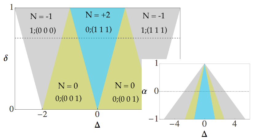
where ${\Delta=(\varepsilon_{c}-\varepsilon_{f})/2(t_{\parallel}^{c}-t_{\parallel}^{f})}$ is the normalized distance between centers of the bands (i.e. $\varepsilon_{c}-\varepsilon_{f}$) and $v_{\perp}$ the hybridization intensity perpendicular to the symmetry plane. We also assumed that the anisotropy $\delta$ affects equally the hopping parameters $t_{\parallel/\perp}^{c,f}$ of $c$- and $f$-electrons within/perpendicular to the symmetry plane, i.e. $\delta=t^{c}_{\perp}/t_{\parallel}^{c}$ and $t^{f}_{\perp}=\delta t_{\parallel}^{f}$. The resulting phase-diagram is shown in Fig. 2 for completely localized $f$-electrons, $t_{\parallel}^{f}=t_{\perp}^{f}=0$. Just below each winding number signalized in the phase diagram we also show the topological indices $\nu_{0};(\nu_{1}\nu_{2}\nu_{3})$ following Fu and Kane notation in Ref. [30]. The white regions are trivial phases with $0$ in all topological invariants.

Candidate-compounds for topological Kondo insulators are formed from magnetic ions with ground states involving odd-parity orbitals. Concentrating onto the rare-earth 3⁺-ions with partially filled $4f$ shell, Ce-, Sm-, and Yb-based materials are of potential interest. The ground state Kramers’ doublet in case of the former two compounds arises from the 5/2-sextet and in case of the latter from the 7/2-octet. The necessary requirement for the appearance of a Kondo insulator as discussed here is then a crystal field which stabilizes the $\Gamma^{J}_{1/2}$-doublet in the ground state. Looking at representations of all possible point groups and their basis functions [39], we notice that from the $f$-electron multiplets a pure $\Gamma^{J}_{1/2}$-doublet only separates in tetragonal or hexagonal crystal symmetries. Specifically, the $\Gamma^{5/2}_{1/2}$-doublet is allowed as one possible ground state in all tetragonal lattices and some of the hexagonal lattices, while the $\Gamma^{7/2}_{1/2}$-doublet can only be a ground state in some of the hexagonal lattices. Table 1 summarizes the possible point group symmetries of lattices allowing for a Kondo insulator derived from the $5/2$- and $7/2$-multiplets, respectively.

We conclude that Ce- and Sm-based Kondo insulators can only have $\Gamma^{J}_{1/2}$-doublet ground state in tetragonal or hexagonal structures. One specific Ce-compound with tetragonal point group symmetry D_2d, to which our above analysis applies is CeRu₄Sn₆ [40]. Recent x-ray spectroscopy experiments in combination with band structure calculations indicate that the $\Gamma^{5/2}_{1/2}$-doublet is the lowest energy state and inversion of bands occurs [41, 42, 43]. Moreover, the $4f$ occupancy near to integer value $n_{f}\sim 1$ and the low dispersive $f$-band, put this material into the topologically interesting region $|N|=2$ of the phase diagram, Fig. 2. All known Sm-based Kondo insulators, on the other hand, have cubic symmetry and our analysis does not apply. Finally, Kondo insulators based on Yb can only exhibit $\Gamma^{J}_{1/2}$-doublet ground state in the four hexagonal symmetries indicated in table 1. Among the established Yb based Kondo insulators there is none with hexagonal symmetry, i.e. these compounds can at most be realized in low-order neighbor approximation. Recently, an interesting Yb compound with hexagonal symmetry, YbNi₃$X_{9}$ ($X=$ Al, Ga), has been synthesized, but it appears to be metallic [44].

Besides the rare-earth elements, Kondo insulators may also be find in metal transition elements, for instance the new Iridium-based compound Sr₂IrO₄[45] has a narrow $5d$ band from Ir which hybridizes with $4p$ band from Oxygen. It also shows a $\Gamma^{J}_{1/2}$-doublet ground state and has a tetragonal lattice structure.

We have studied $3D$ Kondo insulators, where a wide conduction band hybridizes with a degenerate Kramers’ doublet of localized $f$-electrons. We have shown that in cases where the doublet is that of lowest angular momentum projection, $m_{J}=\pm 1/2$, the symmetry of orbitals involved allows for an improved characterization of the topological properties. The existence of an underlying low-energy effective field theory for three-dimensional ($3D$) topological insulators guarantees that the electromagnetic and thermal responses are associated with topological invariants. Here the clean system is connected with a fine-tuned Hamiltonian in class DIII, which in turn is characterized by the $\mathbb{Z}$-invariant. In this case, the winding number distinguishes the chirality of Dirac cones at the surfaces, providing further informations about the edge states. Shiozaki et al. [46] have investigated the possible realizations of physical quantities which distinguish the $\mathbb{Z}_{2}$ properties from the $\mathbb{Z}$ ones.

As an example, in cases where the band width of conduction electrons sets the largest energy scale, the tetragonal topological Kondo insulator is in a nontrivial phase with winding number $|N|=2$, which means that we have two Dirac cones with the same chirality at each surface. Moreover, the phase diagram of this Kondo insulator shows a new weak topological phase when increasing the hopping anisotropy from the cubic to tetragonal structure. When other than the $m_{J}=\pm 1/2$-doublet is involved in the hybridization or when the crystalline field is other than one of those listed in table 1, such system may only appear in a low order neighbor approximation.

Relevant crystal structures for this work are thus those which allow for a pure $\Gamma^{J}_{1/2}$ doublet in the ground state. This implies that topological Kondo insulators involving Kramers’ doublets from the $7/2$ spin-orbit octet can only exist in some of the crystalline hexagonal lattices (see table 1). Kondo insulators forming from hybridization with a Kramers’ doublets from the $5/2$-sextet, on the other hand, can exist in all tetragonal and some of the hexagonal lattices. In practice, the crystal field splitting may not be strong enough to separate the ground state and (anisotropic) pressure may help to stabilize a topological phase. Finally, we have discussed several implications for the rare-earth compounds.

The authors thank the extensive discussions with T.Micklitz and T.O.P. thanks helpful comments from P.Aynajian and S.Kirchner. This work was supported by Brazilian Research Agencies CNPq and FAPERJ, and Chinese Agency NSFC under grant numbers 11750110429 and U1530401, and Chinese Research Center CSRC.

References

- [1] M. Dzero, K. Sun, V. Galitski, and P. Coleman, Phys. Rev. Lett. 104, 106408 (2010).
- [2] T. Takimoto, Journal of the Physical Society of Japan 80, 123710 (2011).
- [3] M. Dzero, K. Sun, P. Coleman, and V. Galitski, Phys. Rev. B 85, 045130 (2012).
- [4] M. Fruchart and D. Carpentier, Comptes Rendus Physique 14, 779 (2013).
- [5] M. Dzero and V. Galitski, Journal of Experimental and Theoretical Physics 117, 499 (2013).
- [6] D. J. Kim, J. Xia, and Z. Fisk, Nature Materials 13, 466 (2014).
- [7] G. Li, Z. Xiang, F. Yu, T. Asaba, B. Lawson, P. Cai, C. Tinsman, A. Berkley, S. Wolgast, Y. S. Eo, D.-J. Kim, C. Kurdak, J. W. Allen, K. Sun, X. H. Chen, Y. Y. Wang, Z. Fisk, and L. Li, Science 346, 1208 (2014).
- [8] M. Dzero, J. Xia, V. Galitski, and P. Coleman, Annual Review of Condensed Matter Physics 7, 249 (2016).
- [9] V. Alexandrov, M. Dzero, and P. Coleman, Phys. Rev. Lett. 111, 226403 (2013).
- [10] M. Legner, A. Rüegg, and M. Sigrist, Phys. Rev. B 89, 085110 (2014).
- [11] P. P. Baruselli and M. Vojta, Phys. Rev. B 90, 201106 (2014).
- [12] P. P. Baruselli and M. Vojta, Phys. Rev. Lett. 115, 156404 (2015).
- [13] M. Legner, A. Rüegg, and M. Sigrist, Phys. Rev. Lett. 115, 156405 (2015).
- [14] N. Xu, P. K. Biswas, J. H. Dil, R. S. Dhaka, G. Landolt, S. Muff, C. E. Matt, X. Shi, N. C. Plumb, M. Radović, E. Pomjakushina, K. Conder, A. Amato, S. V. Borisenko, R. Yu, H. M. Weng, Z. Fang, X. Dai, J. Mesot, H. Ding, and M. Shi, Nature Communications 5, 4566 EP (2014).
- [15] Y. Zhong, Y.-F. Wang, H.-T. Lu, and H.-G. Luo, Phys. Rev. B 88, 235111 (2013).
- [16] T. Yoshida, R. Peters, S. Fujimoto, and N. Kawakami, Phys. Rev. B 87, 165109 (2013).
- [17] J. Werner and F. F. Assaad, Phys. Rev. B 88, 035113 (2013).
- [18] G. Baskaran, ArXiv e-prints (2015), arXiv:1507.03477 [cond-mat.str-el] .
- [19] A. Thomson and S. Sachdev, Phys. Rev. B 93, 125103 (2016).
- [20] A. M. Lobos, A. O. Dobry, and V. Galitski, Phys. Rev. X 5, 021017 (2015).
- [21] Zhong, Yin, Liu, Yu, and Luo, Hong-Gang, Eur. Phys. J. B 90, 147 (2017).
- [22] Inversion symmetry restricts the diagonal blocks of in orbital-space to be even, and off-diagonal hybridization blocks to be odd functions in . In presence of time reversal-symmetry, , this excludes Pauli-spin matrices on the orbital diagonal blocks of , while restrictions on hybridization blocks are different for symmetric and anti-symmetric hybridization combinations , i.e. symmetric elements involve Pauli spin-matrices while anti-symmetric elements are independent of spin orientations. Notice that the choice of a relative phase-factor between and -electrons, for which is of the indicated form, is reflected in coefficients in Eq. (3), and one may alternatively work in a basis where .
- [23] T. Yamada and Y. Ono, Physical Review B Rev. B 85, 165114 (2012).
- [24] I.e. without negative signs in the first line, and , now purely real/imaginary numbers for odd/even.
- [25] For it is the matrices with .
- [26] A. P. Schnyder, S. Ryu, A. Furusaki, and A. W. W. Ludwig, Phys. Rev. B 78, 195125 (2008).
- [27] M. Sato and Y. Ando, Reports on Progress in Physics 80, 076501 (2017).
- [28] See appendix, where we review the Brouwer index, give details on hybridization-matrices, discuss the tetragonal Kondo insulator, and exemplify a non-zero winding number with spin textures in cubic structures.
- [29] Such perturbations change class DIII to AIII without modifying its characterizing topological invariant.
- [30] L. Fu and C. L. Kane, Physical Review B 76, 045302 (2007).
- [31] The renormalization factor is e.g. found from expanding the self-energy due to interaction between localized -electrons close to the Fermi surface [3], or alternatively using slave bosons [32] or Gutzwiller’s approximation [33, 34].
- [32] H. Kusunose, S. Yotsuhashi, and K. Miyake, Phys. Rev. B 62, 4403 (2000).
- [33] T. M. Rice and K. Ueda, Phys. Rev. Lett. 55, 995 (1985a).
- [34] T. M. Rice and K. Ueda, Phys. Rev. Lett. 55, 2093 (1985b).
- [35] G. Rosenberg and M. Franz, Phys. Rev. B 82, 035105 (2010).
- [36] J. I. Väyrynen and G. E. Volovik, JETP Letters 93, 344 (2011).
- [37] S. Shen, Topological Insulators: Dirac Equation in Condensed Matters, Springer Series in Solid-State Sciences, Vol. 174 (Springer, 2013).
- [38] E. Fradkin, Field Theories of Condensed Matter Physics, 2nd ed. (Cambridge University Press, 2013).
- [39] C. J. Bradley and A. P. Cracknell, The mathematical theory of symmetry in solids: representation theory for point groups and space groups (Oxford Clarendon Press, 1972).
- [40] S. Paschen, H. Winkler, T. Nezu, M. Kriegisch, G. Hilscher, J. Custers, A. Prokofiev, and A. Strydom, Journal of Physics: Conference Series 200, 012156 (2010).
- [41] M. Sundermann, F. Strigari, T. Willers, H. Winkler, A. Prokofiev, J. M. Ablett, J.-P. Rueff, D. Schmitz, E. Weschke, M. M. Sala, A. Al-Zein, A. Tanaka, M. W. Haverkort, D. Kasinathan, L. H. Tjeng, S. Paschen, and A. Severing, Scientific Reports 5, 17937 (2015).
- [42] M. Sundermann, K. Chen, Y. Utsumi, Y.-H. Wu, K.-D. Tsuei, J. Haenel, A. Prokofiev, S. Paschen, A. Tanaka, L. H. Tjeng, and A. Severing, Journal of Physics: Conference Series 807, 022001 (2017).
- [43] For a DMFT-study on this compound, discussing the temperature dependence on the selecting ground state, see e.g. Ref. [47].
- [44] T. Yamashita, R. Miyazaki, Y. Aoki, and S. Ohara, Journal of the Physical Society of Japan 81, 034705 (2012).
- [45] B. J. Kim, H. Jin, S. J. Moon, J.-Y. Kim, B.-G. Park, C. S. Leem, J. Yu, T. W. Noh, C. Kim, S.-J. Oh, J.-H. Park, V. Durairaj, G. Cao, and E. Rotenberg, Phys. Rev. Lett. 101, 076402 (2008).
- [46] K. Shiozaki and S. Fujimoto, Phys. Rev. Lett. 110, 076804 (2013).
- [47] P. Wissgott and K. Held, The European Physical Journal B 89, 5 (2016).
- [48] M.-T. Tran, T. Takimoto, and K.-S. Kim, Phys. Rev. B 85, 125128 (2012).
Appendix A Winding number and Brouwer index
For convenience of the reader we here review the calculation of the winding number, , via the Brouwer degree, Eq. (7) in the main text. Starting out from the Hamiltonian matrix and the chiral symmetry operator , we use anti-commutation relation, , to simplify terms, e.g. , etc. One then arrives at , with , which can be cast into the form