New closures for more precise modeling
of Landau damping in the fluid framework

Fluid models are an extremely important tool in many areas of space physics and astrophysics. Despite the underlying dynamics of these systems being often almost completely collisionless, theoretical models and numerical simulations with simplified fluid models that implicitly assume a high-collisionality regime, such as magnetohydrodynamics (MHD) [1, 2, 3, 4, 5], provided deep insight into many phenomena, such as the solar wind, the global structure of the heliosphere, turbulence theories, magnetic reconnection and many others. The implicit assumption of high collisionality in MHD comes from prescribing the pressure to be a scalar quantity, i.e., by prescribing that the underlying distribution function is strictly isotropic and that it remains strictly isotropic during its time evolution. In collisionless systems, the distribution function is free to evolve from its initial state and become anisotropic, before micro-instabilities start to regulate/restrict its further anisotropic evolution. In another words, the implicit assumption of high-collisionality in MHD comes from prescribing the pressure fluctuations to be isotropic. The absence of anisotropic pressure fluctuations in compressible MHD is the main reason why MHD deviates (even at the linear level for an isotropic Maxwellian), from the simplest collisionless fluid description, known as CGL (after Chew, Goldberger and Low [6, 7, 8, 9, 10]) and also sometimes referred to as collisionless MHD. Nevertheless, even in the low-frequency long-wavelength limit, the CGL fluid model still deviates from a collisionless kinetic description, primarily because of the absence of the kinetic effect of Landau damping [11]. For example, consider a proton-electron plasma with external magnetic field $\bm{B}_{0}$, where both species are described by an equilibrium bi-Maxwellian distribution function, and consider the usual ion-acoustic (sound) mode that propagates in the direction parallel to $\bm{B}_{0}$. At wavelengths that are much longer than the Debye length, the exact kinetic dispersion relation reads

where the plasma response function $R(\zeta)=1+\zeta Z(\zeta)$ and the plasma dispersion function $Z(\zeta)=\frac{1}{\sqrt{\pi}}V.P.\int_{-\infty}^{\infty}\frac{e^{-x^{2}}}{x-\zeta}dx+i\sqrt{\pi}e^{-\zeta^{2}}$ $\forall$ $\textrm{Im}(\zeta)$, and the integration passes “through” the pole. With species index $r$, the variable $\zeta_{r}$ is here defined as $\zeta_{r}=\omega/(|k_{\parallel}|v_{\textrm{th}\parallel r})$, $\omega$ being frequency and $k_{\parallel}$ the parallel wavenumber, the parallel thermal speed $v_{\textrm{th}\parallel r}=\sqrt{2T_{\parallel r}^{(0)}/m_{r}}$, and $T_{\parallel r}^{(0)}=p_{\parallel r}^{(0)}/n_{r}^{(0)}$ is the parallel equilibrium temperature. The dispersion relation (1) can in general be solved only numerically, and for example for $\tau\equiv T_{\parallel e}^{(0)}/T_{\parallel p}^{(0)}=1$, the solution is $\zeta_{p}=\pm 1.457-0.627i$. The negative imaginary part represents strong Landau damping, and since no dispersive effects are present, the Landau damping of the parallel ion-acoustic mode does not disappear even on large astrophysical scales, i.e. in the low-frequency long-wavelength limit where the phase speed $\omega/k_{\parallel}$ is constant. In contrast, the solution for an ion-acoustic mode with both species described by the CGL pressure equations reads $\zeta_{p}=\pm\sqrt{\frac{3}{2}\frac{(1+\tau)}{(1+\mu)}}$, where $\mu\equiv m_{e}/m_{p}=1/1836$, so for $\tau=1$ the solution is $\zeta_{p}=\pm 1.732$. Alternatively, if the electrons are prescribed to be isothermal, the dispersion relation reads $\zeta_{p}=\pm\sqrt{\frac{1}{2}\frac{(3+\tau)}{(1+\mu)}}$, which for $\tau=1$ yields $\zeta_{p}=\pm 1.414$. Therefore, without Landau damping the usual fluid models do not represent the correct long-wavelength limit of collisionless kinetic theory.

The incorporation of Landau damping into the CGL fluid model was pioneered by Hammett and Perkins [12] and was further refined (for example [13, 14, 15, 16, 17] and references therein). These fluid models that describe Landau damping in the fluid framework are usually referred to as gyrofluids (formulated in the guiding-center reference frame) or Landau fluids (formulated in the usual laboratory reference frame), even though there are other subtle differences and the vocabulary is not strictly enforced. These fluid models are constructed by calculating the hierarchy of fluid moments of the Vlasov equation to higher-orders than the usual pressure tensor, and by finding a closure, where the last retained fluid moment is expressed through lower-order moments. To find a closure, the exact kinetic $R(\zeta)$ function is replaced by a suitable Padé approximant (as a ratio of two polynomials) in such a way, that the closure is valid for all $\zeta$ values. A (generalized) n-pole Padé approximant $R_{n}(\zeta)$ to a function $R(\zeta)$ is found by matching the power series expansion $|\zeta|\ll 1$ and the asymptotic series expansion $|\zeta|\gg 1$ of both functions. There are of course many possible choices, and here we are interested only in approximants that at least reproduce the first term of the asymptotic expansion $R(\zeta)=-1/(2\zeta^{2})+\cdots$, i.e. as having a precision $o(\zeta^{-2})$. Here we define “the basic” n-pole Padé approximant of $R(\zeta)$ as

where the second index in $R_{n,n^{\prime}}(\zeta)$ signifies, that $n^{\prime}$ additional asymptotic points were used in comparison with the basic $R_{n,0}(\zeta)$ definition. The $n^{\prime}=0$ index helps to quickly orient a large hierarchy of many possible $R(\zeta)$ approximants. This asymptotic profile correctly captures the asymptotic decay of the density moment, and any profile with fewer asymptotic points should be avoided if possible. The 1-pole approximant is $R_{1}(\zeta)=1/(1-i\sqrt{\pi}\zeta)$. $R_{n,0}(\zeta)$ has power series precision $o(\zeta^{2n-3})$ and asymptotic series precision $o(\zeta^{-2})$, so $R_{n,n^{\prime}}(\zeta)$ has precision $o(\zeta^{2n-3-n^{\prime}})$ and $o(\zeta^{-2-n^{\prime}})$. The Padé approximant to $Z(\zeta)$ is defined as $R_{n,n^{\prime}}(\zeta)=1+\zeta Z_{n,n^{\prime}}(\zeta)$. Comparison with the 2-index notation of Martín et al. [18] (introducing superscript M) and of Hedrick and Leboeuf [19] (superscript HL) can be done easily according to $Z_{n,n^{\prime}}^{M}=Z_{\frac{n+n^{\prime}}{2},n^{\prime}-3}$ and $Z_{n,n^{\prime}}^{HL}=Z_{n,n^{\prime}+n-3}$. Padé approximants were also used in developing analytic models for the Rayleigh-Taylor and Richtmyer-Meshkov instability [20, 21].

Similarly to [12], we concentrate here on a 1D geometry that can be viewed as an electrostatic case, or from our view preferably as propagation along $B_{0}$, which naturally picks up the ion-acoustic mode (since the 1D velocity fluctuations are along $B_{0}$). For brevity we drop writing the parallel subscripts (except on $k_{\parallel}$) and species index $r$, since closures are constructed independently for each species. Examples of $R(\zeta)$ Padé approximants are $R_{2,0}(\zeta)=1/(1-i\sqrt{\pi}\zeta-2\zeta^{2})$,

$R_{3,1}(\zeta)=\frac{1-i\frac{4-\pi}{\sqrt{\pi}}\zeta}{1-\frac{4i}{\sqrt{\pi}}\zeta-2\zeta^{2}+2i\frac{4-\pi}{\sqrt{\pi}}\zeta^{3}}$. We note that Table 1 of [19] can be recovered analytically, and we report a typo in their $a_{1}$ coefficient for $Z_{3,1}(\zeta)$ that should be $a_{1}=\frac{2}{4-\pi}=2.32990$ instead of $2.23990$, used for example in [15]. The two Padé approximants used by [12] read $R_{3,2}(\zeta)=\frac{1-\frac{i\sqrt{\pi}}{2}\zeta}{1-\frac{3i\sqrt{\pi}}{2}\zeta-2\zeta^{2}+i\sqrt{\pi}\zeta^{3}}$;

where the first choice yields a closure for the heat flux $q^{(1)}=-i\frac{2}{\sqrt{\pi}}n_{0}v_{\textrm{th}}\textrm{sign}(k_{\parallel})T^{(1)}$. Note that our definition of the thermal speed contains a factor of 2. The second choice yields a closure for $\widetilde{r}$ defined as $r=3p^{2}/\rho+\widetilde{r}$ where the 4-th order moment $r=m\int(v-u)^{4}fd^{3}v$ (we follow the notation of [15]; $\widetilde{r}$ can be also denoted as $\delta r$) and the $R_{4,3}(\zeta)$ closure obtained by [12] reads

Curiously, it can be shown that the fluid dispersion relation that uses the above closure, is equivalent to the kinetic dispersion relation (1) once the exact $R(\zeta)$ is replaced by the approximant $R_{4,3}(\zeta)$ (strictly speaking it is equivalent to the numerator of (1) once both terms in (1) are written with common denominator). Electron inertia must be considered and the displacement current must of course be neglected in the fluid model to yield (1). This observation is also true for all other $R_{n,n^{\prime}}(\zeta)$ closures presented here and closures that satisfy (1) can be viewed as “reliable” or physically-meaningful.

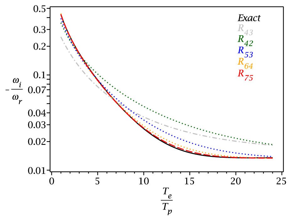
In Figure 1, the dispersion relation of the fluid model that uses the above $R_{4,3}(\zeta)$ closure (gray dot-dashed line) is compared to the exact kinetic solution (1) (black solid line). The figure is motivated by Figure 9.18 in [22] (page 355). A closure is called “static” when the last retained moment (i.e. $\widetilde{r}$) is directly expressed through lower order moments. A closure is called “time-dependent” or “dynamic”, when the closure involves $\partial/\partial t$ of the last retained moment (i.e. $\zeta\widetilde{r}$), and the $\partial/\partial t$ is then replaced by a $d/dt$ to recover the Galilean invariance. Time-dependent closures can be constructed usually with a higher-order Padé approximant than static closures, however, the replacement of $\partial/\partial t$ with $d/dt$ introduces only one nonlinearity among other neglected nonlinearities.

Here we report on the most precise Landau fluid closures that can be constructed at a given level. For example, by using $R_{3,1}(\zeta)$, the following static closure can be constructed for the heat flux

Considering power series precision (henceforth abbreviated as p.s.p.), this is the most precise static closure that can be constructed for the heat flux, and the precision is $o(\zeta^{2})$. The coefficients of the $R_{4,2}(\zeta)$ approximant are $b_{3}=-2a_{1}$; $b_{2}=3a_{2}-2$; $a_{1}=-i\frac{\sqrt{\pi}(10-3\pi)}{(3\pi-8)}$; $a_{2}=-\frac{(16-5\pi)}{(3\pi-8)}$; $b_{1}=-i\frac{2\sqrt{\pi}}{(3\pi-8)}$, and the static closure with the highest p.s.p., $o(\zeta^{3})$, that can be constructed at the 4th-moment level reads

The $R_{4,2}(\zeta)$ is also used to obtain the dynamic closure for the heat flux with the highest p.s.p., and written for a change in real space, the closure reads

The $\mathcal{H}$ operator is the negative Hilbert transform operator that acts on a function $f(z)$ according to $\mathcal{H}f(z)\equiv-\frac{1}{\pi z}*f(z)\equiv-\frac{1}{\pi}V.P.\int_{-\infty}^{\infty}\frac{f(z^{\prime})}{z-z^{\prime}}dz^{\prime}$, the $*$ operator being the convolution. We use the Fourier decomposition $e^{-i\omega t+ik_{\parallel}z}$, and the transformation of a closure between Fourier and real space can be done simply according to $-i\omega\leftrightarrow\partial/\partial t$; $ik_{\parallel}\leftrightarrow\partial_{z}$; $i\textrm{sign}(k_{\parallel})\leftrightarrow\mathcal{H}$, and $|k_{\parallel}|\leftrightarrow-\partial_{z}\mathcal{H}$. The closure is plotted in Figure 1 as a dark green dotted line and the closure is very accurate in the region $\tau=[1,5]$.

A closure that has the highest p.s.p. at the 4th-moment level, $o(\zeta^{4})$, is a dynamic closure constructed with approximant $R_{5,3}(\zeta)$, that has coefficients $b_{5}=-2a_{3}$; $b_{4}=-2a_{2}$; $b_{3}=3a_{3}-2a_{1}$; $b_{2}=3a_{2}-2$, $a_{1}=\frac{i}{\sqrt{\pi}}\frac{(27\pi^{2}-126\pi+128)}{3(9\pi-28)}$; $a_{2}=\frac{(33\pi-104)}{3(9\pi-28)}$; $a_{3}=\frac{i}{\sqrt{\pi}}\frac{2(9\pi^{2}-69\pi+128)}{3(9\pi-28)}$; $b_{1}=-\frac{i}{\sqrt{\pi}}\frac{2(21\pi-64)}{3(9\pi-28)}$, and the closure reads

The dispersion relation of a fluid model that uses the $R_{5,3}(\zeta)$ closure is plotted in Figure 1 as a blue dotted line. In the region $\tau=[1,5]$, this is the most precise closure that can be constructed at the 4th-moment level.

In contrast, a static closure that uses the most asymptotic series $|\zeta|\gg 1$ points at the 4th-moment level, with precision $o(\zeta^{-6})$, is constructed with $R_{4,4}(\zeta)$, and the closure reads $\widetilde{r}^{(1)}=-\frac{3}{4}\sqrt{\pi}v_{\textrm{th}}\mathcal{H}q^{(1)}$. The most asymptotically precise closure is a dynamic closure constructed with $R_{5,6}(\zeta)$, that has a precision $o(\zeta^{-8})$ and the closure reads $\big[\frac{d}{dt}-\frac{8}{3\sqrt{\pi}}v_{\textrm{th}}\partial_{z}\mathcal{H}\big]\widetilde{r}^{(1)}=-2v_{\textrm{th}}^{2}\partial_{z}q^{(1)}$. For temperatures $\tau=[15,100]$, this is the most precise closure that can be constructed at the 4th-moment level.

We mapped all the possible Landau fluid closures that can be constructed (at the level of heat flux or the moment $\widetilde{r}$) and there are 7 possible static closures (5 reliable), and 13 dynamic closures (9 reliable), some of them related. We do not provide analytic solutions for all of these closures. Nevertheless, other notable closures are for $R_{5,4}(\zeta)$: $\big[\frac{d}{dt}-\frac{21\pi-64}{\sqrt{\pi}(9\pi-28)}v_{\textrm{th}}\partial_{z}\mathcal{H}\big]\widetilde{r}^{(1)}=-n_{0}v_{\textrm{th}}^{3}\frac{256-81\pi}{2(9\pi-28)\sqrt{\pi}}\partial_{z}\mathcal{H}T^{(1)}-v_{\textrm{th}}^{2}\frac{32-9\pi}{2(9\pi-28)}\partial_{z}q^{(1)}$, and for $R_{5,5}(\zeta)$: $\big[\frac{d}{dt}-\frac{6\sqrt{\pi}}{(32-9\pi)}v_{\textrm{th}}\partial_{z}\mathcal{H}\big]\widetilde{r}^{(1)}=-v_{\textrm{th}}^{2}\frac{9\pi}{2(32-9\pi)}\partial_{z}q^{(1)}.$

All the above closures are also applicable to a 3D geometry when written for $\widetilde{r}_{\parallel\parallel},q_{\parallel},T_{\parallel},u_{\parallel}$. Considering the gyrotropic limit, the closure for $\widetilde{r}_{\perp\perp}$ defined as $r_{\perp\perp}=2p_{\perp}^{2}/\rho+\widetilde{r}_{\perp\perp}$ is simply $\widetilde{r}_{\perp\perp}=0$. The $\widetilde{r}_{\parallel\perp}$ is defined as $r_{\parallel\perp}=p_{\parallel}p_{\perp}/\rho+\widetilde{r}_{\parallel\perp}$, and introducing for brevity $\mathcal{T}_{\perp}\equiv\frac{T_{\perp}^{(1)}}{T_{\perp}^{(0)}}+\Big(\frac{T_{\perp}^{(0)}}{T_{\parallel}^{(0)}}-1\Big)\frac{B_{z}}{B_{0}}$, there are 2 static closures, for $R_{1}(\zeta)$: $q_{\perp}^{(1)}=-\frac{p_{\perp}^{(0)}}{\sqrt{\pi}}v_{\textrm{th}\parallel}\mathcal{H}\mathcal{T}_{\perp}$, and for $R_{2,0}(\zeta)$: $\widetilde{r}_{\parallel\perp}^{(1)}=-\frac{\sqrt{\pi}}{2}v_{\textrm{th}\parallel}\mathcal{H}q_{\perp}^{(1)}$, which up to replacing $B_{z}$ with $|\bm{B}|$ (that comes here from a complete linearization), are equivalent to the closures of [14]. There are also 6 dynamic closures, some of them related. With 3-pole approximants, a closure can be constructed for $R_{3,1}(\zeta)$: $\big[\frac{d}{dt}-\frac{\sqrt{\pi}}{4-\pi}v_{\textrm{th}\parallel}\partial_{z}\mathcal{H}\big]\widetilde{r}_{\parallel\perp}^{(1)}=-v_{\textrm{th}\parallel}^{2}\frac{\pi}{2(4-\pi)}\partial_{z}q_{\perp}^{(1)}$, and for $R_{3,2}(\zeta)$: $\big[\frac{d}{dt}-\frac{2}{\sqrt{\pi}}v_{\textrm{th}\parallel}\partial_{z}\mathcal{H}\big]\widetilde{r}_{\parallel\perp}^{(1)}=-v_{\textrm{th}\parallel}^{2}\partial_{z}q_{\perp}^{(1)}$, that in the vanishing Larmor radius limit are equivalent to closures of [15]. Here we report on a new closure that is constructed with $R_{3,0}(\zeta)$:

that has a higher p.s.p., $o(\zeta^{3})$. No closures with 4-pole (or higher) approximants are possible for $\widetilde{r}_{\parallel\perp}$.

Returning to a 1D geometry and considering closures at higher-order moments $X_{n}=m\int(v-u)^{n}fdv$, the closure for $X_{5}$ with the highest p.s.p., $o(\zeta^{5})$, is constructed with $R_{6,4}(\zeta)$, and reads

The closure is plotted in Figure 1 as the orange dotted line. Going higher in the fluid hierarchy, and decomposing $X_{6}=15p^{3}/\rho^{2}+\widetilde{X}_{6}$, the closure with the highest p.s.p., $o(\zeta^{6})$, is obtained with $R_{7,5}(\zeta)$, being

with coefficients

The closure is plotted in Figure 1 as the red line.

The remarkable result that the reliable closures reproduce the exact kinetic dispersion relation (1) once $R(\zeta)$ is replaced by $R_{n,n^{\prime}}(\zeta)$ leads us to conjecture that there exist reliable fluid closures that can be constructed for even higher moments, i.e. satisfying (1), once $R(\zeta)$ is replaced by the $R_{n,n^{\prime}}(\zeta)$ approximant. Furthermore, for a given n-th order fluid moment, the reliable closure with the highest power series precision is the dynamic closure constructed with $R_{n+1,n-1}(\zeta)$. Indeed, for higher order fluid moments one should be able to construct closures with higher order $R_{n+1,n-1}(\zeta)$ approximants that will converge to $R(\zeta)$ with increasing precision. Thus, one can reproduce linear Landau damping in the fluid framework to any desired precision, which establishes the convergence of fluid and collisionless kinetic descriptions.

The convergence was shown here in 1D geometry for the example of a long-wavelength low-frequency ion-acoustic mode. Nevertheless, the 1D closures have general validity, i.e. from the largest astrophysical scales to the Debye length, and are of course valid also for the Langmuir mode. However, there are limitations in modeling the Langmuir mode, since for $k_{\parallel}\lambda_{D}<0.2$, Landau damping disappears very quickly, and some closures show a small positive growth rate instead.

The next logical step would be to establish an analytic convergence of fluid and kinetic descriptions in a 3D geometry in the gyrotropic limit. However, in 3D, for a given n-th order tensor $\bm{X}_{n}$, the number of its gyrotropic moments is equal to $1+\textrm{int}[n/2]$ and increases with $n$. Therefore, it might be more difficult to show the convergence in 3D, although the convergence should exist.

Concerning direct applicability of the derived closures, numerical simulations of turbulence show a peculiar behavior, in that at sub-proton scales, the parallel velocity spectrum is always much steeper in kinetic simulations than Landau fluid simulations (e.g. Fig. 7 of [23]). The $r_{\parallel\parallel}$ closure of [12], does not include coupling with the parallel velocity component, whereas our new closures do and could explain the discrepancy.

Finally, to emphasize the importance of the closures obtained, consider 1-fluid models in 1D geometry with $k_{\parallel}\lambda_{D}\ll 1$, closed by a simple Maxwellian (non-Landau fluid) closures $X_{n}=0$, for $n$ odd, $n\geq 3$; and $X_{n}=(n-1)!!\frac{p^{n/2}}{\rho^{n/2-1}}$, for $n$ even, $n\geq 4$ (or that the deviation $\widetilde{X}_{n}=0$ for $n$ even). It can be shown by induction that the dispersion relation reads

For $n=3$ the solution is $\zeta=\pm\sqrt{3/2}$, and $n=4$ yields $\zeta=\pm\sqrt{3/2+\sqrt{3/2}}$, $\zeta=\pm\sqrt{3/2-\sqrt{3/2}}$. However, $n=5$ yields $\zeta=\pm(\frac{15}{4})^{1/4}$; $\zeta=\pm i(\frac{15}{4})^{1/4}$, and $n=6$ yields $\zeta=\pm 0.58$; $\zeta=\pm 1.75$; $\zeta=\pm 1.87i$. In fact, for $n>4$, the solution of (10) will always yield modes that are unstable, and such fluid models can not be used for numerical simulations. The closure for $n=4$, $r=3p^{2}/\rho$, is sometimes called the “normal” closure [24]. Here we conclude that the “normal” closure is actually the last non-Landau fluid closure, and that beyond the 4th-order moment, Landau fluid closures are required.