Neural Networks as Artificial Specifications
Abstract
In theory, a neural network can be trained to act as an artificial specification for a program by showing it samples of the programs executions. In practice, the training turns out to be very hard. Programs often operate on discrete domains for which patterns are difficult to discern. Earlier experiments reported too much false positives. This paper revisits an experiment by Vanmali et al. by investigating several aspects that were uninvestigated in the original work: the impact of using different learning modes, aggressiveness levels, and abstraction functions. The results are quite promising.
Keywords:
neural network for software testing, automated oraclesNOTICE: This is a pre-print of the same paper published in the proceedings of the 30th International Conference on Testing Software and Systems (ICTSS) 2018, LNCS. Publisher: Springer-Nature. DOI: https://doi.org/10.1007/978-3-319-99927-2_11. Additional results have also been added in the Appendix which were not included in the published version due to the space limitation.
1 Introduction
Nowadays, many systems make use of external services or components to do some of their tasks, allowing services to be shared, hence reducing cost. However, we also need to take into account that third parties services may be updated on the fly as our system is running in production. If such an update introduces an error, this may affect the correctness of our system as well. One way to guard against this is by doing run time verification [2]: at the runtime the outputs of these services are checked against their formal specifications. Unfortunately, in practice it is hard to persuade developers to write formal specifications.
A more pragmatic idea is to use ’artificial specifications’ generated by a computer. Another use case is automated testing. Tools like QuickCheck, Evosuite, and T3 [3, 6, 13] are able to generate test inputs, but if no specification is given, only common correctness conditions such as absence of crashes can be checked. Using artificial specifications would extend their range.
Although we cannot expect a computer to be able to on its own specify the intent of a program, it can still try to guess this intent. One way to do this is by observing some training executions to predict general properties of the program, e.g. in the form of ’invariants’ (state properties) [5], finite state machine [12], or algebraic properties [4]. These approaches cannot however capture the full functionality of a program, e.g. [5] can only infer predefined families of predicates, many are simple predicates such as such as and . With respect to these approaches, neural networks offer an interesting alternative, since they can be trained to simulate a function [9].
The trade off of using artificial specifications is the additional overhead in debugging. When a production-time execution violates such a specification, the failure may be either caused by an error triggered by the execution, or by an error in the training executions that were reflected in the predictions, or due to inaccuracy of the predictions. The first two cases expose errors (though the second case would take more effort to debug). However, the failure in the last case is a false alarm (false positive). Since we do not know upfront if a violation is a real error or a false positive, we will need to investigate it (debugging), which is quite labour intensive. If it turns out to be a false positive, the effort is wasted. Despite the potential, studies on the use of neural networks as artificial specifications are few: [16, 1, 11, 10]. They either reported unacceptably high rate of false positives, or do not address the issue.
In this paper we revisit an experiment by Vanmali et al. [16] that revealed rate of false positives —a rate of above 5% is likely to render any approach unusable in practice. The challenge lies in the discrete nature of the program used as the experiment subject, making it very hard to train a neural network. This paper explores several aspects that were left uninvestigated in the original work, namely the influence of different learning modes, aggresiveness levels, and abstraction. The results are quite promising.
2 Neural Network as an Artificial Specification
Consider a program that behave as a function . An artificial specification is a predicate ; means that ’s output is judged as correct, and else incorrect. With respect to the intended specification , ’s judgment is a true positive is when both and judge a T, a true negative is when they agree on the judgement F, a false positive is when judges and judges , and a false negative is when judges and judges .
An neural network (NN) is a network of ’neurons’ [9] that behaves as a function . We will restrict ourselves to feed forward NNs (FNNs) where the neurons are organized in linearly ordered layers [9]; an example is below:
The first layer is called the input layer, consisting of neurons connected to the inputs. The last layer is the output layer, consisting of neurons that produce the outputs. The layers in between are called hidden layers. An input neuron simply passes on its input, else it has inputs and an additional input called ’bias’ whose value is always 1 [9]. Each input connector has a weight . The neuron’s output is the weighted sum of its inputs, followed by applying a so-called activation function: . A commonly used is the logistic function, which we also use in our experiments.
Any continuous numeric function , restricted within any closed subset of , can be simulated with arbitrary accuracy by an FNN [7], which implies that an FNN can indeed act as an artificial specification for , if is injectable into such a numeric function. That is, there exists a continuous numeric function and injections and such that encodes : for all , . However, finding a right FNN is hard. A common technique to find one is by training an FNN using a set of sample inputs and outputs, e.g. using the back propagation [9] algorithm. It might be easier to train the NN to simulate instead, where is some chosen abstraction on ’s output values. The trade off is that we get a weaker specification.
Since an NN does not literally produce a bool, we couple its output vector to a so-called comparator to calculate the judgement by comparing with the observed output . Basically, if their values are ’far’ from each other, then the judgement is , and else . By adjusting what ’far’ means we can tune the specification’s aggressiveness without having to tamper with the NN’s internals. In our experiments (below), the identity function will be used as the injector and . Because simply passes on its input, it will be omitted from the formulas.
3 Experiments
Figure 1 shows a credit approval program from the financial domain that was used as the experiment subject by Vanmali et al [16]. The program takes 8 input parameters describing a customer. The output is a pair where is a boolean indicating whether the credit request is approved, and if so specifies the maximum allowed credit. We will ignore since [16] already shows that an FNN can accurately predict its value. Despite its size, the subject is quite challenging for an NN to simulate because it operates on a discrete domain (the numeric values are all integers). The whole input domain has 224000 possible values. We will use an FNN with 8 inputs (representing ’s inputs) and a hidden layer with 24 neurons (adding more layers and neurons does not really improve the FNN’s accuracy).
Five variations of the FNN will be used, as listed below, along with the used comparator . is parameterized with aggressiveness level (integer 0 (least aggressive) … 5) that determines ’s policy to deal with non clear-cut cases.
- 1.
The FNN has one output, which is trained to simulate . Its comparator uses Euclidian distance, with sensitivity linearly scaled by : , with .
- 2.
The FNN has outputs, trained to simulate . The abstraction maps approve’s output to a vector representing one of uniform sized intervals in ’s range [0..18000], such that the -th interval is represented by a vector of 0’s except a single 1 at the -th position. If , let be the index of the greatest element in .
The comparator is more complicated. An obvious case is when and report the same winner. If the NN’s winner is confident of itself, ’s output is judged as correct. When they produce different winners and the NN’s winner is confident of itself, we judge to be incorrect. Other cases are non-clear-cut and judged depending on the aggressiveness level. The full definition of is shown below. The original work Vanmali et al. [16] only uses aggressiveness level.
function ();end functionThe thresholds and are set to .
- 3.
The FNN is a less presumptuous variant of , with set to . This will cause more cases to be regarded as non-clear-cut.
- 4.
The FNN is like , but trained to simulate . is used to ’stretch’ to divide into finer intervals in the lower region of ’s range, e.g. if we believe the region to be more error prone, and growing coarser towards the other end. We use the log function to do this: with and controlling the steepness.
- 5.
The FNN is like , but trained to simulate . is used to ’stretch’ to divide into finer intervals in the center region of ’s range. We use logistic function where (’s maximum) and determines the function’s steepness.
Training. We randomly generate 500 distinct inputs (from the space of 224000 values) and collect the corresponding ’s outputs. This set of 500 pairs (input,output) forms the training data. For every type of FNN above and every aggressiveness level an FNN is trained. controls the granularity of the used abstraction, so we also try various (10..60). For each FNN, the connections’ weight is randomly initialized in . The training is done in a series of epochs using the back propagation algorithm [9]. We tried both the incremental learning mode [9, 8], where the FNN’s error is propagated back after each training input, and batch learning modes, where only the average error is propagated back, after the whole batch of training inputs (500 of them). Incremental learning is thus more sensitive to the influence of individual inputs.
Evaluation. To evaluate the FNNs’ ability to detect errors, we run them on 21 erroneous variations (mutants) of the subject as in [16] —they are listed in the Appendix. For each mutant, 500 distinct random inputs are generated, whose outputs are ’error exposing’ (distinguishable from the corresponding outputs of the correct subject). As an artificial specification, an FNN should ideally reject all these error exposing outputs. Each rejection is a true positive. We also generate 500 distinct random inputs and feed it to the (unmutated) subject. The FNN should accepts the corresponding outputs —each rejection is a false positive.
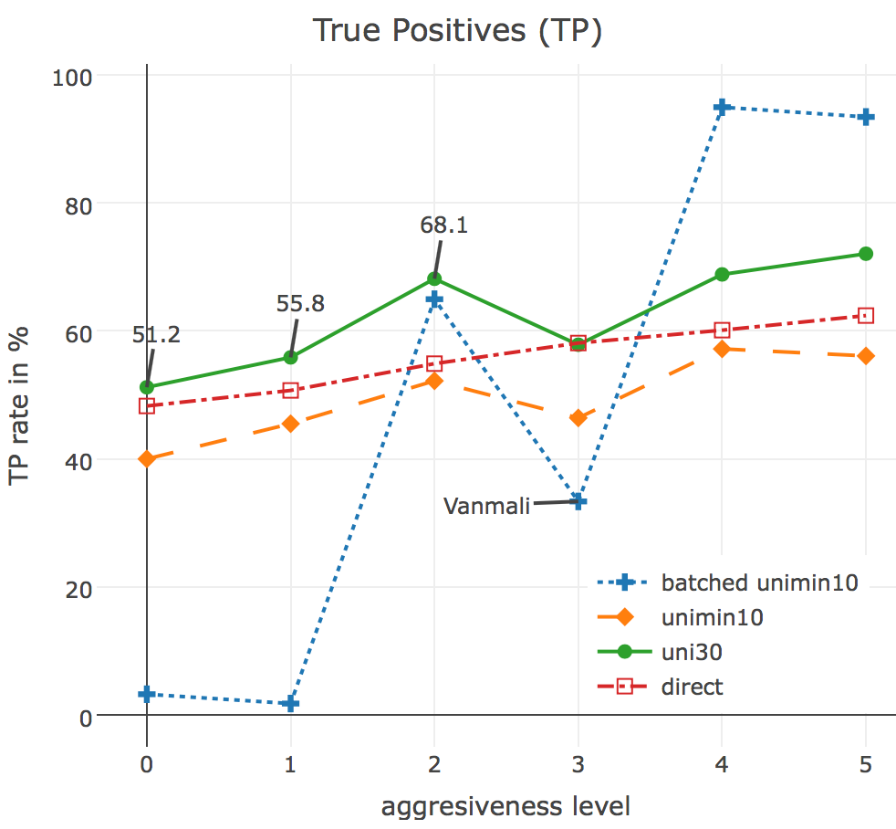
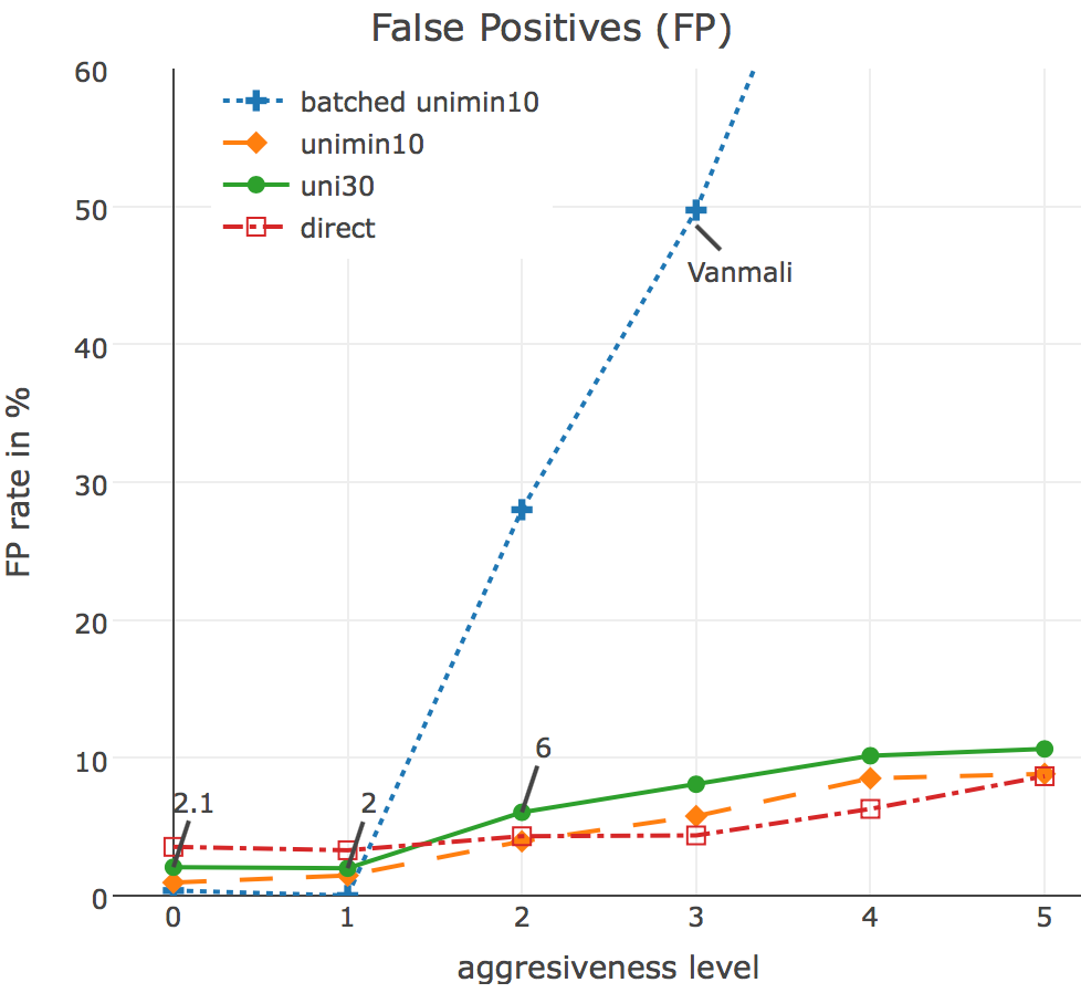
Figure 2 shows some of the results. Except for , the training was done in 1500 epochs with learning rate 0.5. We can see that using abstraction improves the FNN’s performance: compare with . The latter obtains a true positive rate 68% on aggressiveness 2, implying that out of two erroneous executions, is likely to detect at least one, while when the aggressiveness level is set low, its rate of false positives is only around 2%. Abstraction also makes training easier: after 1500 epochs produces a mean square error (MSE) of , whereas the shown results for is obtained after 10000 epochs (incrementally) with 0.1 learning rate, yielding an MSE .
The experiment in [16] uses . We believe [16] used batch learning because the reported MSE after 1500 epochs matches, namely . However, as can be seen in Figure 2, this leads to poor performance (). Incremental learning yields a much more accurate FNN ( MSE), hence also better performance (). The performance of the FNN in [16] under our setup is indicated by the -markers in Figure 2.
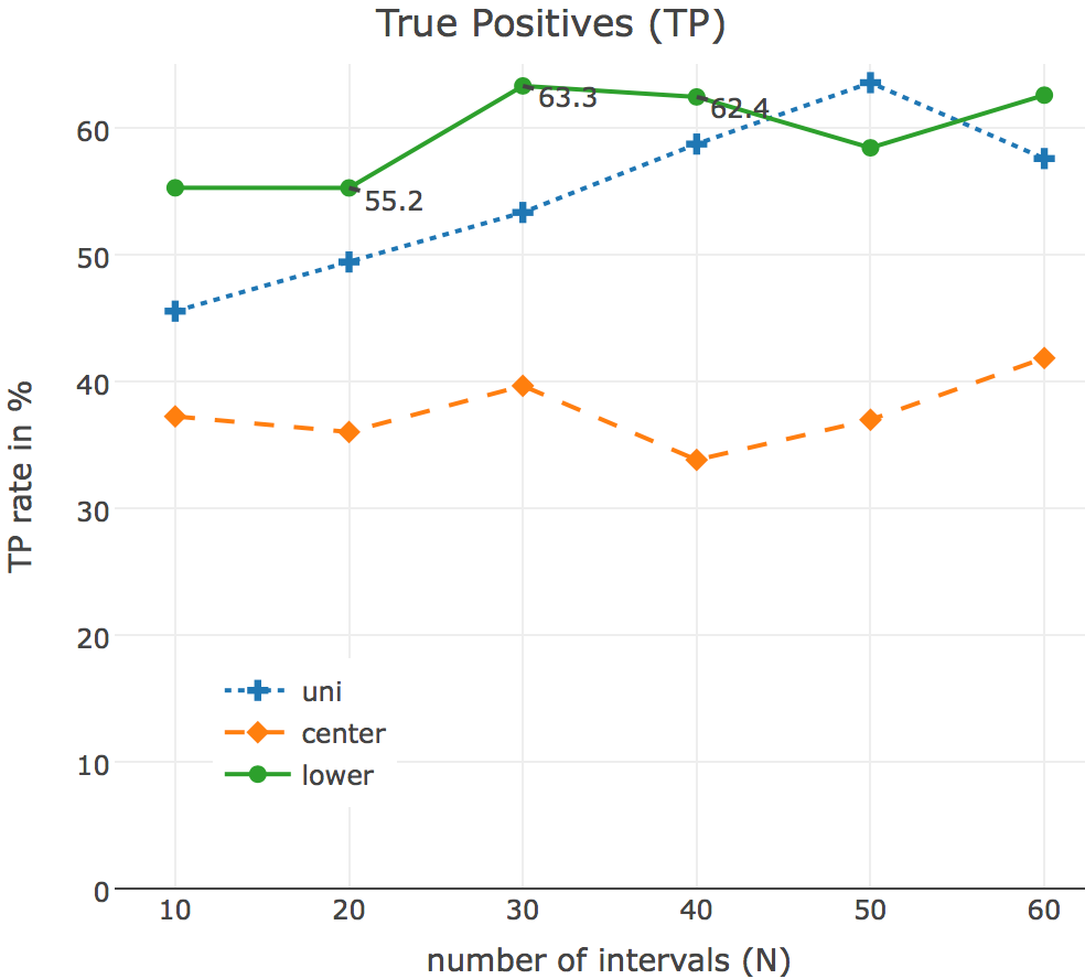
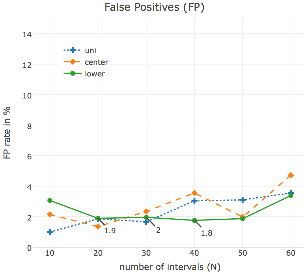
The effect of using different abstractions and abstraction granularity (the parameter) is shown in Figure 3. Based on the results in Figure 2, we now use the lowest aggressiveness level (0). The graph of shows that increasing can greatly improve the FNN’s ability to detect error, while keeping the false positive rate below 5%. We also see and perform significantly better than , implying that the choice of the abstraction function matters. Compared to , and introduce non-linear granularity. The results suggest that introducing more granularity in the region (of ’s output) which are more error prone pays off.
4 Conclusion
The experiment showed that, contrary to earlier attempts, it is possible to train Neural Networks, given an appropriate abstraction, to become an artificial specification for a non-trivial program with acceptable precision. As future work, more case studies are needed to see how this generalizes.
References
- [1] Aggarwal, K., Singh, Y., Kaur, A., Sangwan, O.: A neural net based approach to test oracle. ACM SIGSOFT Software Engineering Notes 29(3), 1–6 (2004)
- [2] Cao, T.D., Phan-Quang, T.T., Felix, P., Castanet, R.: Automated runtime verification for web services. In: Int. Conf. on Web Services (ICWS). IEEE (2010)
- [3] Claessen, K., Hughes, J.: QuickCheck: a lightweight tool for random testing of Haskell programs. In: ACM Sigplan Int. Conf. on Functional Programming (2000)
- [4] Elyasov, A., Prasetya, W., Hage, J., Rueda, U., Vos, T., Condori-Fernández, N.: AB=BA: Execution equivalence as a new type of testing oracle. In: 30th ACM Symposium on Applied Computing. ACM (2015)
- [5] Ernst, M., Perkins, J., Guo, P., McCamant, S., Pacheco, C., Tschantz, M., Xiao, C.: The Daikon system for dynamic detection of likely invariants. Science of Computer Programming 69(1), 35–45 (2007)
- [6] Fraser, G., Arcuri, A.: Evosuite: Automatic test suite generation for object-oriented software. In: SIGSOFT FSE. pp. 416–419 (2011)
- [7] Goodfellow, I., Bengio, Y., Courville, A.: Deep learning. MIT Press (2016)
- [8] Joelself: FANN C# NeuralNet float, http://joelself.github.io/FannCSharp
- [9] Kriesel, D.: A brief Introduction on Neural Networks. dkriesel.com (2007)
- [10] Lu, Y., Ye, M.: Oracle model based on RBF neural networks for automated software testing. Information Technology Journal 6(3), 469–474 (2007)
- [11] Mao, Y., Boqin, F., Li, Z., Yao, L.: Neural networks based automated test oracle for software testing. In: Neural Information Processing. pp. 498–507. Springer (2006)
- [12] Mariani, L., Pastore, F.: Automated identification of failure causes in system logs. In: 19th Int. Symp on Software Reliability Engineering. IEEE (2008)
- [13] Prasetya, I.S.W.B.: T3i: A tool for generating and querying test suites for java. In: 10th Joint Meeting on Foundations of Software Engineering (FSE). ACM (2015)
- [14] Prasetya, I.: T3: Benchmarking at third unit testing tool contest. In: Proceedings of the Eighth International Workshop on Search-Based Software Testing. pp. 44–47. IEEE Press (2015)
- [15] Tillmann, N., De Halleux, J.: Pex–white box test generation for. net. In: International conference on tests and proofs. pp. 134–153. Springer (2008)
- [16] Vanmali, M., Last, M., Kandel, A.: Using a neural network in the software testing process. International Journal of Intelligent Systems 17(1), 45–62 (2002)
Appendix 0.A Results on Individual Mutations
The table below shows each of the mutation used in our experiment for simulating errors. The mutations are the same as originally used in [16].
| line | mutation | ||||
|---|---|---|---|---|---|
| 2: |
| ||||
| 3: Age<18 |
| ||||
| 5: Citizenship==0 |
| ||||
| 7: State==0 |
| ||||
| 8: |
| ||||
| 11: Marital==0 |
| ||||
| 12: Dependents>0 |
| ||||
| 15: Sex==0 |
| ||||
| 20: Marital==0 |
| ||||
| 21: Dependents>2 |
| ||||
| 24: Sex==0 |
|
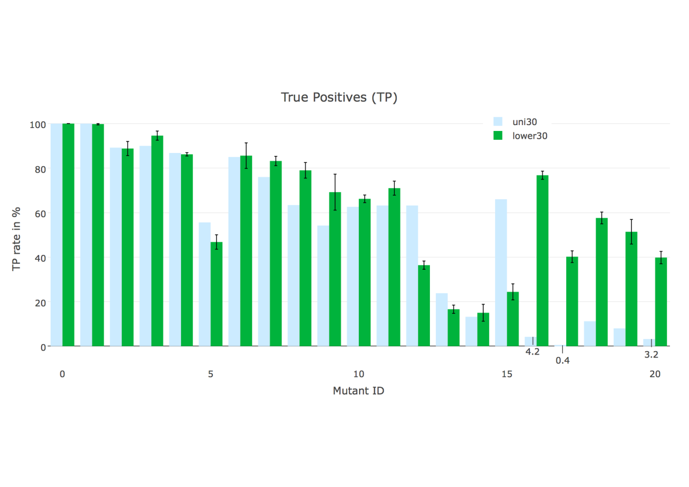
Figure 4 shows the true positive and false positive rates of the FNNs on individual mutants. Two results of two FNNs are shown. The first is with its aggressiveness level set to 0; recall that uses the function as the abstraction function. The second is , with aggressiveness 0, but it uses as the abstraction.
Let’s first consider the true positives (top graph). We see here that on mutants M16, M17, and M20 actually performs very poorly. See the top graph in Figure 4 —’s results on these three cases are annotated in the graph.
In contrast, the hardest mutants for are M13 and M14, but even on these mutants has a true positive rate of . Whether this 10% is good enough depends on the situation. We have defined the rate of true positives as the percentage of wrong executions that the FNN judges as wrong as well. In particular, note that the metric is not defined as the percentage of mutations that can be discovered. If we would define it like this, would have 100% rate of true positives because with enough test cases eventually it will be able to detect all mutants. So, individual rate of true positives for e.g. M14 means thus that if we manage to trigger at least 10 distinct executions that expose the mutation, statistically the FNN has a good chance to detect at least one of them, and thus identifying the mutation. While this sounds very encouraging, note that the actual probability for detecting the error also depends on the probability of producing executions that expose it. In the experiments, the probability of the latter is simply 1: we knew upfront that there is a mutation, so generating the set of error exposing executions for each mutant was not problematic. In a real regression testing setup, it is not possible to steer the testing process towards exposing a particular error; we do not even know upfront if the new version of the program would contain any regression error at all. There are indeed tools to automatically generate test inputs capable of generating a large number of test cases [3, 14]. However, it is hard to generate test cases that are evenly distributed over all control paths in the target program. Some paths may even be left uncovered because they are too difficult to cover, even by tools that employ more sophisticated techniques like an evolutionary algorithm [6] or symbolic calculation [15].
 |
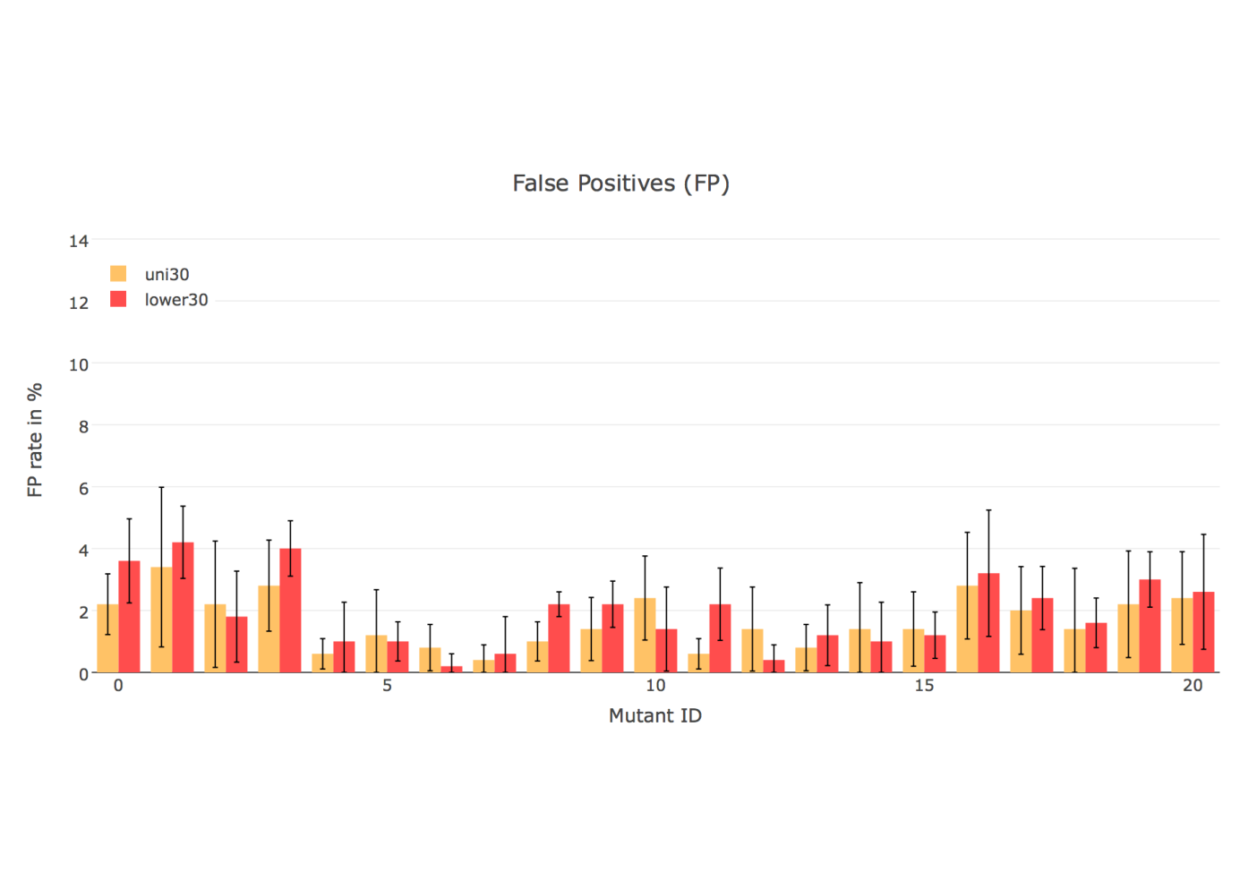 |
The bottom graph in Figure 4 shows the individual false positive rate of and . Each bar in this graph also has its own error bar to indicate the standard deviation of the value the bar represents (the error bar is capped above at 100 and below at 0, since true/false positive rates can only range between [0..100]). For each mutant , and each experiment (e.g. ), the error of the false positive rate of the experiment is calculated by randomly dividing the set of 500 executions used in the experiment, into 5 bags of 100 elements and then we calculate the false positive rate of the experiment with respect to each bag. is defined as the standard deviation of these values. The error bars indicate that sometimes the false positive rate can peak above 5%, though in average both configurations, and , produce rates that are below , for every individual mutant.