Linear Parameter Varying Representation of a class of MIMO Nonlinear Systems

The static nonlinearity that is present in the nonlinear model needs to be factorized to obtain an LPV representation. Multiple factorization approaches are possible. Here, the nonlinear function $f(z(t))$ is decomposed as $\bar{f}(z(t))z(t)+c$.

Denote $\mathbb{P}$ as the set of values that can be reached by $z(t)$ for a specified class of inputs $u(t)\in\mathbb{U}$ with $t\in[0\>\infty)$ and initial conditions $x(0)\in\mathbb{X}$.

This assumption excludes for instance functions $f(z(t))$ that have singularities in the region of interest (e.g. $\frac{1}{z}$, if $z=0$ lies within the range of interest). Note that decomposition of a function in the form given in Assumption 2 is non-unique. The function $\bar{f}(z(t))$, $\mathbb{R}^{n_{z}}\rightarrow\mathbb{R}^{n_{w}\times n_{z}}$ is called the scheduling map in the sequel.

Assumption 3 is only required for the offset propagation algorithm. If no constant offset ($f(0)=0$) is present in the static nonlinearity, this assumption is not required. Note that this assumption does not impose stability of the total NLFR system.

Under Assumptions 2 and 3, the NLFR structure with $D_{\mathrm{zw}}=0$ can be represented by:

where:

where $G^{[i]}_{0}$ is obtained by evaluating the steady-state gain of $G^{[i]}(s)$, i.e. $G^{[i]}_{0}=\lim_{s\rightarrow 0}G^{[i]}(s)$. Eq. (7) to hold, all ${G_{0}^{[2]}}^{-1}{G_{0}^{[4]}}$ and $\left(G_{0}^{[3]}+G_{0}^{[1]}{G_{0}^{[2]}}^{-1}{G_{0}^{[4]}}\right)$ should exist and be finite. In the case $n_{z}\leq n_{u}$ and the rank of $G_{0}^{[2]}$ is equal to $n_{z}$, the Moore-Penrose left-inverse of the matrix $G_{0}^{[2]}$ can be used (Golub and Van Loan, 1996). This is however a conservative requirement. It suffices that the following assumption holds:

Under Assumption 4 one can always find a vector $d$ such that $G_{0}^{[2]}d=G_{0}^{[4]}c$, resulting in the following offset mitigation equations:

Note that Assumption 4 is only required for the offset propagation algorithm.

The constant offset at both the input and the output can be dealt with during the LPV control design process as a disturbance or by using input or output trimming methods.

The time-dependent notation $z(t)$ is simplified to $z$ to lighten the notation in this section.

This subsection introduces a systematic approach to perform the factorization $\tilde{f}(z)=\bar{f}(z)z$ for $z\in\mathbb{P}$. One can write:

This assumption holds, for example, for all continuously differentiable functions $\mathcal{C}_{1}^{n_{w}}(\mathbb{R}^{n_{z}})$.

Under assumptions 2 and 5, the functions $\bar{f}_{i}$ are given by:

and

It can be observed that for a polynomial (or rational) function $\tilde{f}(z)$, also the functions $\bar{f}_{i}(z_{1},z_{2},\ldots,z_{i})$ are polynomial (rational) (remember that $\tilde{f}(z)$ never contains a constant term: $\tilde{f}(0)=0$).

In case the function $\tilde{f}(z)$ is not partially differentiable in the points of interest, but its left and right derivative are finite in those points, the partial derivatives can be replaced by a finite constant without introducing a singularity in $\bar{f}(z)$. However, the continuity of $\bar{f}(z)$ is lost.

The proposed factorization is not unique. By changing the order in which the variables $z_{i}$ are considered, different factorizations of the multivariate nonlinearity could be obtained.

Under Assumption 2 we can represent the NLFR structure as an LPV affine state-space representation with an additional constant offset at the input and/or output:

where $p(t)$ is given by the scheduling map:

This results in the following affine state-space LPV structure:

with:

Note that the expressions in Eq. (17) are linear in $p(t)$.

The resulting affine state-space LPV representation is not unique, a state transformation can be introduced. Also the latent variables $z(t)$ and $w(t)$ are non-uniquely defined, similar to the non-uniqueness that is present in block-oriented systems (Schoukens et al., 2015; Schoukens, 2015). This non-uniqueness can be further explored for the scheduling variables selection. From a control design point of view it is desirable for the scheduling signals $p(t)$ or the input of the static nonlinearity $z(t)$ to be measurable or observable. This will be explored in future research.

Note that the proposed algorithm, including the constant offset removal and the nonlinear function factorization can be completely automated starting from a NLFR representation. However, in some cases it can be worthwhile to search for an ’optimal’ factorization. As discussed above, multiple factorizations of a multivariate nonlinear function are possible. Hence, the search for an ’optimal’ factorization is more difficult to automate and requires more study.

A 2-DOF mass-spring-damper system with unit masses ($M_{1}=M_{2}=1$ in Figure 2) a nonlinear spring $\kappa(y_{1})$ and nonlinear position-dependent damping $\gamma(y_{1},\dot{y}_{1})$ is considered:

where the nonlinear damping and spring are given by:

with $k_{1}=\pi^{2}$, $k_{2}=(1.2\pi)^{2}$, $k_{3}=10$, $c_{1}=0.1$, $c_{2}=0.01$, $c_{3}=0.1$, $c_{4}=10$, $c_{5}=0.2$.

A NLFR representation can be obtained using the notation as in Eq. (1):

where

and

where $z_{i}$ denotes the $i$-th entry from the vector $z$ and the matrices $D_{\mathrm{zw}}$, $D_{\mathrm{zu}}$, $D_{\mathrm{yw}}$, $D_{\mathrm{yu}}$ are all zero matrices.

It can be observed that no offset handling is required since it holds for the nonlinearity in the NLFR that $f(0)=0$.

Multiple factorizations are possible using the factorization scheme presented in this paper. By first factorizing $z_{1}$, and $z_{2}$ next, we obtain:

Note that the functions $k_{3}z_{1}^{2}$ and $c_{3}\sin(c_{4}z_{1})+c_{5}z_{2}$ are the resulting scheduling maps of the LPV embedding.

Another possibility (first factorize $z_{2}$, and $z_{1}$ next) is:

Many more factorizations are possible, beyond the ones obtained with the proposed factorization scheme. For instance:

for any finite $\alpha$ results in an equivalent representation.

Using the choice (23), the equivalent LPV representation of the considered system is given by:

where

with $p_{1}(t)=\bar{f}_{1}(q_{1}(t))$, $p_{2}(t)=\bar{f}_{2}(q_{1}(t),\dot{q}_{1}(t))$ provided in Eq. (23).

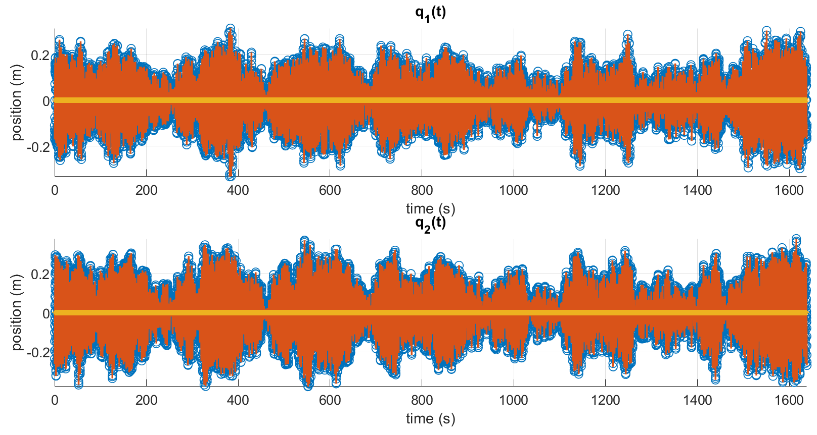
The output responses of the NLFR representation and by the embedding obtained LPV representation are depicted in the time- and frequency domain in Figures 3 and 4 respectively. A perfect match between both can be observed.

The scheduling signals $p$ are obtained by applying the scheduling map on the trajectories $x$ and $u$ obtained by the nonlinear simulation.

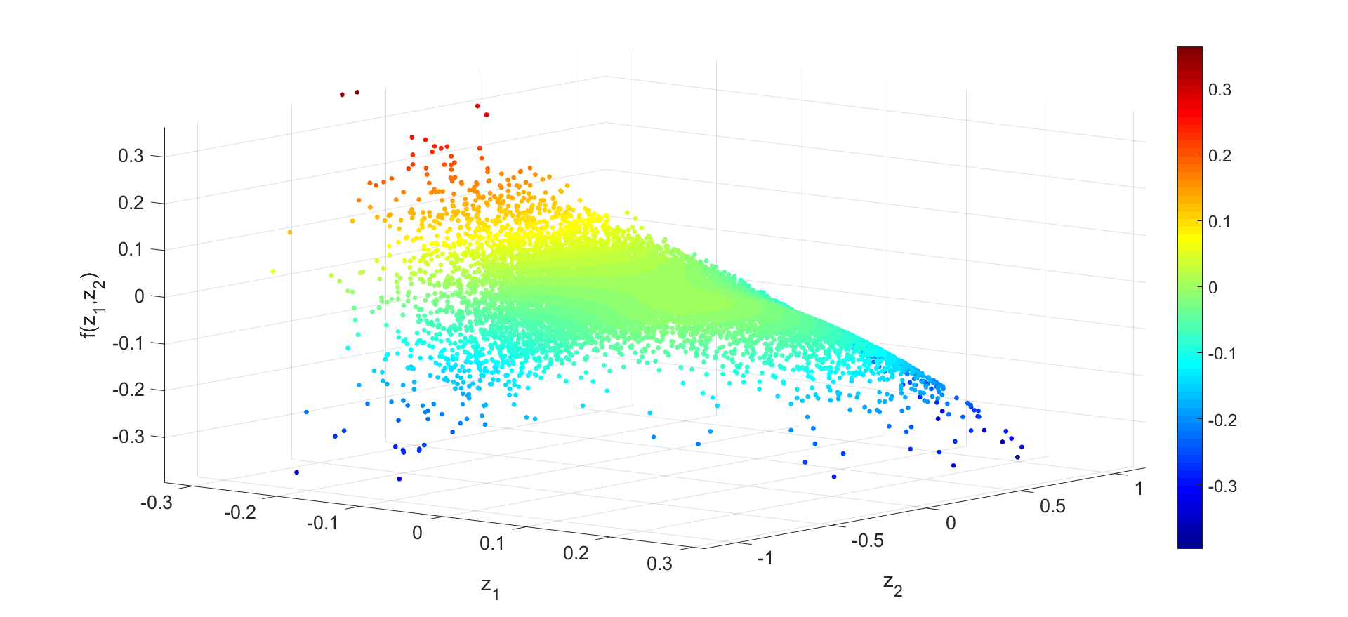
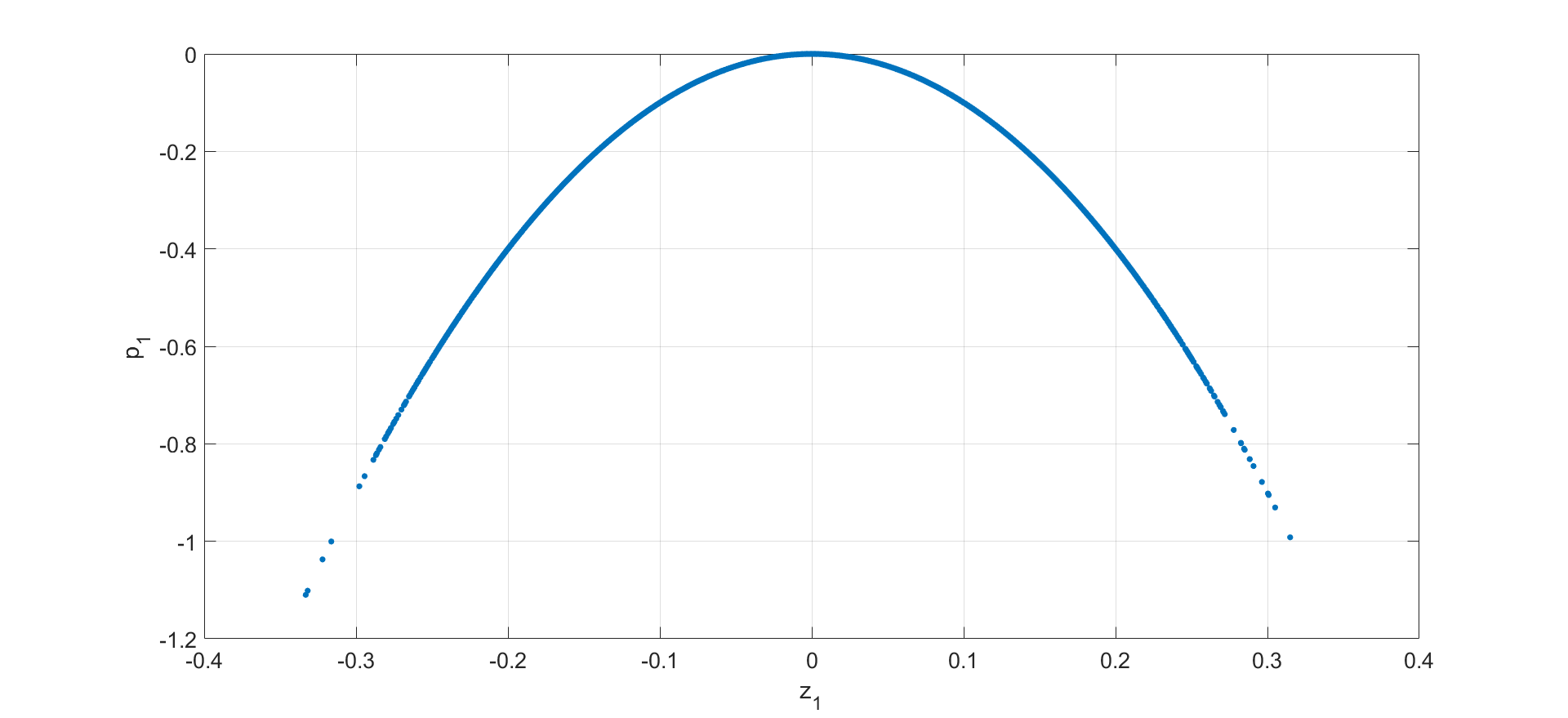
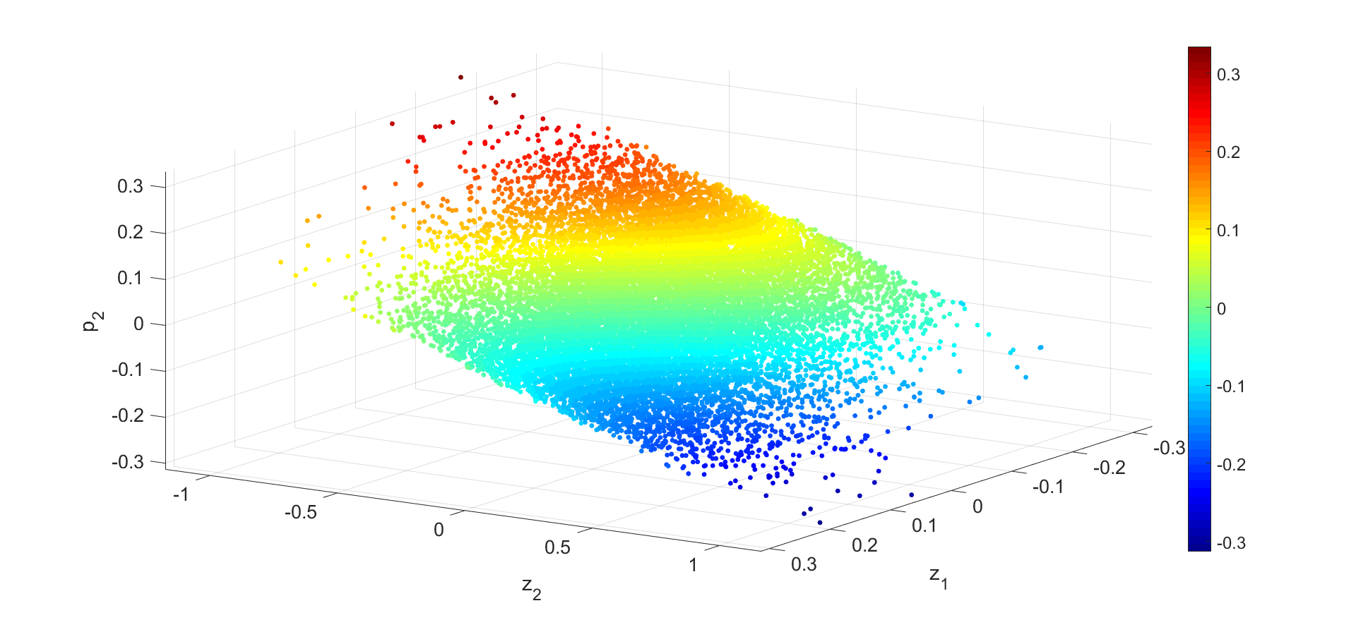
The system nonlinearity that is present in the NLFR representation (see Figure 5) is factorized in 2 nonlinear functions $\bar{f}_{1}(z_{1})$, $\bar{f}_{2}(z_{1},z_{2})$ shown in Figures 6 and 7 respectively.

References

- Abbas et al. (2017) Abbas, H., Hanema, J., Tóth, R., Mohammadpour, J., and Meskin, N. (2017). An improved robust model predictive control for linear parameter-varying input-output models. International Journal of Robust and Nonlinear Control, 28(3), 859–880.
- Abbas et al. (2014) Abbas, H., Tóth, R., Petreczky, M., Meskin, N., and Mohammadpour, J. (2014). Embedding of nonlinear systems in a linear parameter-varying representation. In 19th World Congress of the International Federation of Automatic Control, 6907–6913. Cape Town, South Africa.
- Chisci et al. (2003) Chisci, L., Falugi, P., and Zappa, G. (2003). Gain-scheduling MPC of nonlinear systems. International Journal of Robust and Nonlinear Control, 13(3-4), 295–308.
- dos Santos et al. (2011) dos Santos, P., Azevedo Perdicoulis, T., Novara, V., Ramos, J., and Rivera, D. (eds.) (2011). Linear Parameter-Varying System Identification: New Developments and Trends. World Scientific, Signapore.
- Giri and Bai (2010) Giri, F. and Bai, E. (eds.) (2010). Block-oriented Nonlinear System Identification, volume 404 of Lecture Notes in Control and Information Sciences. Springer-Verlag, London.
- Golub and Van Loan (1996) Golub, G. and Van Loan, C. (1996). Matrix Computations - Third Edition. Johns Hopkins University Press, Baltimore and London.
- Hanafi et al. (2018) Hanafi, H., Seron, M., and De Doná, J. (2018). Fault estimation and controller compensation in lure systems by LPV-embedding. International Journal of Control, 0(0), 1–14.
- Hsu et al. (2008) Hsu, K., Poolla, K., and Vincent, T.L. (2008). Identification of structured nonlinear systems. IEEE Transactions on Automatic Control, 53(11), 2497–2513.
- Mohammadpour and Scherer (2012) Mohammadpour, J. and Scherer, C. (eds.) (2012). Control of Linear Parameter Varying Systems with Applications. Springer-Verlag, New York.
- Novara et al. (2011) Novara, C., Vincent, T.L., Hsu, K., Milanese, M., and Poolla, K. (2011). Parametric identification of structured nonlinear systems. Automatica, 47, 711–721.
- Piga et al. (2015) Piga, D., Cox, P., Tóth, R., and Laurain, V. (2015). LPV system identification under noise corrupted scheduling and output signal observations. Automatica, 53, 329 – 338.
- Schoukens (2015) Schoukens, M. (2015). Identification of Parallel Block-Oriented Models starting from the Best Linear Approximation. Ph.D. thesis, Vrije Universiteit Brussel, Belgium.
- Schoukens et al. (2015) Schoukens, M., Marconato, A., Pintelon, R., Vandersteen, G., and Rolain, Y. (2015). Parametric identification of parallel Wiener-Hammerstein systems. Automatica, 51(1), 111–122.
- Schoukens and Tiels (2017) Schoukens, M. and Tiels, K. (2017). Identification of block-oriented nonlinear systems starting from linear approximations: A survey. Automatica, 85, 272–292.
- Schoukens and Tóth (2018) Schoukens, M. and Tóth, R. (2018). From nonlinear identification to linear parameter varying models: Benchmark examples. In 18th IFAC Symposium on system identification (SYSID). Stockholm, Sweden.
- Seron and De Doná (2015) Seron, M. and De Doná, J. (2015). On robust stability and set invariance of switched linear parameter varying systems. International Journal of Control, 88(12), 2588–2597.
- Tóth (2010) Tóth, R. (2010). Modeling and Identification of Linear Parameter-Varying Systems, volume 403 of Lecture Notes in Control and Information Sciences. Springer-Verlag, Berlin Heidelberg.
- Vanbeylen (2013) Vanbeylen, L. (2013). Nonlinear LFR Block-Oriented Model: Potential Benefits and Improved, User-Friendly Identification Method. IEEE Transactions on Instrumentation and Measurement, 62(12), 3374–3383.
- Vandersteen and Schoukens (1999) Vandersteen, G. and Schoukens, J. (1999). Measurement and identification of nonlinear systems consisting of linear dynamic blocks and one static nonlinearity. IEEE Transactions on Automatic Control, 44(6), 1266–1271.
- Young (2011) Young, P. (2011). Recursive Estimation and Time-Series Analysis: An Introduction for the Student and Practitioner. Springer-Verlag, Berlin Heidelberg.