Theory of bifurcation amplifiers utilizing the nonlinear dynamical response
of an optically damped mechanical oscillator

We consider an optical cavity mode coupled to a mechanical oscillator with position operator $x$. The coupling is described by the standard radiation pressure interaction $H_{\mathrm{int}}=\hbar g_{0}x\,a^{\dagger}a$, where $g_{0}$ is the single-photon optomechanical coupling rate and $a$ is the photon annihilation operator in the frame rotating at the cavity resonance (angular) frequency $\omega_{r}$. The position operator $x=(c+c^{\dagger})$ is expressed by the phonon annihilation operator $c$ and in units of the zero point motion $x_{\mathrm{zpf}}=\sqrt{\hbar/(2m\omega_{m})}$, where the effective mass is denoted $m$ and the mechanical resonance frequency is $\omega_{m}\ll\omega_{r}$. We let the cavity mode be coherently driven at the frequency $\omega_{r}-\omega_{m}$. We also include a mechanical drive at the oscillator’s resonance frequency.

The dynamics of the system is determined by the quantum Langevin equations

	$\displaystyle\dot{a}$	$\displaystyle=-\frac{\kappa}{2}a-ig_{0}xa+e^{i\omega_{m}t}\Omega+\sqrt{\kappa}\,\xi$		(1)
	$\displaystyle\dot{c}$	$\displaystyle=-\left(\frac{\gamma}{2}+i\omega_{m}\right)c-ig_{0}a^{\dagger}a+e^{-i\omega_{m}t}\Lambda+\sqrt{\gamma}\,\eta$		(2)

where $\kappa$ ($\gamma$) is the energy decay rate of the cavity (oscillator) and we have assumed that the effective mechanical oscillator quality factor is always large. The optical and mechanical drive strengths are denoted $\Omega$ and $\Lambda$, respectively. These rates are proportional to the square root of drive power and they can be considered real and positive without loss of generality. See Figure 1 for an overview of the model parameters.

The operator $\xi(t)$ describes quantum vacuum noise from coupling to external fields and the standard Markovian treatment [27, 28] gives Gaussian noise with $\langle\xi(t)\xi^{\dagger}(t^{\prime})\rangle=\delta(t-t^{\prime})$ and $\langle\xi^{\dagger}(t)\xi(t^{\prime})\rangle=\langle\xi(t)\xi(t^{\prime})\rangle=0$, assuming that the temperature $T$ obeys $k_{B}T\ll\hbar\omega_{c}$. We let the mechanical noise operator $\eta$ obey $\langle\eta(t)\eta^{\dagger}(t^{\prime})\rangle=(n_{\mathrm{th}}+1)\delta(t-t^{\prime})$, $\langle\eta^{\dagger}(t)\eta(t^{\prime})\rangle=n_{\mathrm{th}}$, and $\langle\eta(t)\eta(t^{\prime})\rangle=0$, with the thermal phonon number defined as

$$n_{\mathrm{th}}=\frac{1}{\mathrm{exp}[\hbar\omega_{m}/(k_{B}T)]-1}\ .$$

(3)

We do not consider technical noise in any of the drives, but the theory can easily be extended to include that.

The discussion below will be limited to a particular regime of optical drive powers. The combination of coherent mechanical oscillations and optical power in the cavity gives rise to radiation pressure forces on the mechanical oscillator at all multiples of the mechanical frequency. This includes a DC force which shifts the equilibrium position of the oscillator which in turn shifts the average resonance frequency of the cavity. However, this frequency shift is negligible if we limit ourselves to low enough powers such that

$$\frac{g_{0}^{2}|a_{\mathrm{max}}|^{2}}{\omega_{m}\kappa}\ll 1\ ,$$

(4)

where $a_{\mathrm{max}}=2\Omega/\kappa$ is the cavity amplitude one would get if the optical drive was on cavity resonance and $g_{0}$ was zero. In the limit (4), and for an oscillator with a large quality factor, we can also neglect the response of the mechanical oscillator at higher multiples of the mechanical resonance frequency and only take into account its response at or around its resonance frequency $\omega_{m}$. We consider this regime throughout this article.

We emphasize that the drive parametrized by $\Lambda$ can be realized through optical driving without the need for mechanical actuation. This can be achieved simply by adding an additional optical drive which is modulated at $\omega_{m}$ and thus gives rise to a coherent force on the mechanical oscillator, as was for example done in the study reported in Ref. [14]. However, in Appendix A, we show that to realize the effects described in this article, we would require that this modulated beam drives an auxiliary optical cavity mode whose single-photon coupling to the mechanical oscillator is much smaller than that of cavity mode $a$. This ensures that a sufficiently large value of $\Lambda$ can be realized by optical means without significantly influencing the decay rate $\gamma$ or the mechanical noise properties defined above.

We begin by determining the amplitude and phase of the coherent mechanical oscillations, as well as the coherence of the optical cavity field. Initially, we neglect the thermal and quantum noise, but we will return to the role of fluctuations in Section II.4. As mentioned above, we neglect the mechanical oscillator’s response at higher multiples of $\omega_{m}$. The coherent motion of the mechanical oscillator can then be expressed as

$$x(t)=x_{0}+\bar{r}\cos(\omega_{m}t-\bar{\phi})\ ,$$

(5)

where $x_{0}$ is a shift of the equilibrium position, $\bar{r}$ is the oscillation amplitude and $\bar{\phi}$ is a phase. For convenience, we define the rescaled mechanical amplitude

$$\bar{R}=\frac{g_{0}\bar{r}}{\omega_{m}}\ .$$

(6)

This allows us to express the cavity field as

$$a(t)=\sum_{k}e^{-ik(\omega_{m}t-\bar{\phi})}a_{k}\quad,\quad a_{k}=(-1)^{k-1}\Omega\,e^{i\bar{\phi}}\sum_{n}\chi_{n}J_{n-k}(\bar{R})J_{n+1}(\bar{R})\ ,$$

(7)

where the sums over integers go from minus infinity to plus infinity, we have defined the susceptibilities

$$\chi_{n}=\frac{1}{\kappa/2-in\omega_{m}}\ ,$$

(8)

and $J_{n}(\bar{R})$ is the $n$-th order Bessel function of the first kind. The quantity $a_{k}$ describes the optical coherence at frequency $\omega_{r}+k\omega_{m}$. We now define the standard optomechanical cooperativity

$$C=\frac{4g_{0}^{2}\alpha^{2}}{\kappa\gamma}$$

(9)

where $\alpha=|\chi_{-1}|\Omega$ would be the intracavity coherent amplitude if $g_{0}=0$. The average mechanical amplitude $\bar{r}$ and phase $\bar{\phi}$ can then be determined by the complex, nonlinear, algebraic equation

$$\bar{R}+C\sum_{n}H_{n}J_{n+1}(\bar{R})J_{n}(\bar{R})-e^{-i\bar{\phi}}L=0\ ,$$

(10)

which follows from Equation (2) when defining

$$H_{n}=-\frac{i\kappa\,\chi^{\ast}_{n-1}\chi_{n}}{\omega_{m}|\chi_{-1}|^{2}}\$$

(11)

and the rescaled mechanical drive strength

$$L=\frac{4g_{0}\Lambda}{\gamma\omega_{m}}\ .$$

(12)

We note that the only physical parameter $H_{n}$ depends on is the dimensionless sideband parameter $\omega_{m}/\kappa$.

We now consider the solutions to Equation (10). This equation can be solved numerically by truncating the sum at a sufficiently large integer. Let us focus on the mechanical response to the drive, i.e., on the mechanical amplitude $\bar{R}$ as a function of drive amplitude $L$, which is shown in Figure 2 for different values of the cooperativity $C$ and for a sideband parameter $\omega_{m}/\kappa=10$. We do not show the solution for the phase $\bar{\phi}$, but find that it is small ($|\bar{\phi}|/\pi<0.02$) for all cooperativities and drive strengths in Figure 2. In fact, one can show that $\bar{\phi}=0$ in the resolved sideband limit $\omega_{m}/\kappa\rightarrow\infty$. The Figure shows that for values of the scaled amplitude $\bar{R}$ much less than 1, the mechanical response is linear with an effective damping rate $\gamma(1+C)$. This is due the standard optomechanical damping (or cooling) mechanism, where the radiation pressure interaction leads to an enhanced mechanical decay rate [29, 30, 31]. However, when $\bar{R}$ becomes on the order of unity, the response becomes highly nonlinear. The physical explanation is that the amplitude of the cavity resonance frequency variations then become comparable to $\omega_{m}$, which is on the order of the detuning of the optical beam, such that the optical damping mechanism becomes inefficient.

Increasing the cooperativity beyond a critical value $C_{\mathrm{crit}}$, Figure 2 shows that we get three solutions for $\bar{R}$ for an interval of drive strengths $L_{-}<L<L_{+}$. We will refer to $L_{-},L_{+}$ as bifurcation points or turning points. As we will show in Section II.3, one of the solutions (indicated by a dashed line) is unstable. The system thus displays bistability where two stable solutions exist for the same drive strength $L$. In general, the value of $C_{\mathrm{crit}}$ depends on the sideband parameter $\omega_{m}/\kappa$, but is independent of it in the limit $\omega_{m}/\kappa\gg 1$. In the example shown in Figure 2, we find $C_{\mathrm{crit}}\approx 1.82$. We also see that for even larger values of the cooperativity $C$, the system can display even more solutions, i.e., multistability. The presence of more than one solution means that the system will display hysteresis, i.e, the steady-state mechanical amplitude for a given drive strength will depend on the history of the system. To connect with the theory of optomechanical self-sustained oscillations [13], we reiterate that here we are addressing the dynamical attractor diagram in the red-detuned regime.

To explain the origin of bistability, let us look at the curve for $C=20$ in Figure 2. For large drives, e.g., $L\sim 15$, the lower stable solution where $\bar{R}\sim 1$ describes the case where the optical drive is efficiently driving the cavity mode, such that the mechanical oscillator is efficiently damped. The other stable solution, where $\bar{R}\sim L$, describes the situation where the mechanical amplitude and thus the cavity’s resonance frequency variation is already so large that the optical drive is unable to efficiently address the cavity. The optical damping is then almost absent and only the intrinsic mechanical damping remains. We note that the vanishing of the lower stable solution occurs when the effective frictional force on the oscillator becomes negative. This is because photon down-conversion processes where phonons are created can dominate for large oscillation amplitudes and a sufficient amount of cavity photons. Multistability with more than two stable solutions comes from the fact that for a region of amplitudes, e.g., around $\bar{R}\sim 5$ in Figure 2, the dominant damping mechanism is optical but of a nonlinear nature that corresponds to multi-phonon annihilation processes in the quantum formalism.

There will be optical coherence not only at the original laser frequency, but at all multiples of the mechanical frequency, according to Equation (7). The coherence amplitudes $|a_{k}|$ depend on the steady-state mechanical amplitude $\bar{R}$. For $C>C_{\mathrm{crit}}$, the amplitude will jump from $\bar{R}\sim 1$ to a significantly larger value as the drive strength $L$ is sweeped up from 0 and beyond the bifurcation point where the lower stable solution vanishes. This jump will be accompanied by jumps in the optical coherences $a_{k}$ and can thus easily be monitored optically. The behaviour of optical coherences as $L$ is sweeped up is shown in Figure 3 for $k={-1,0,1}$, $C=20$, and $\omega_{m}/\kappa=10$. We note that the coherences at other values of $k$ are significantly smaller in the resolved sideband limit $\omega_{m}/\kappa\gg 1$.

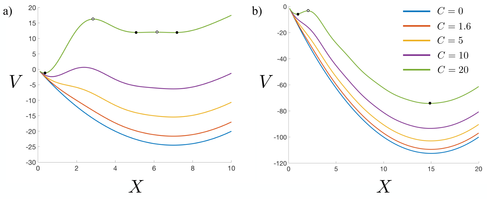
We will now show that, in the resolved sideband limit $\omega_{m}/\kappa\gg 1$, the steady-state solutions for the amplitude $\bar{R}$ can be interpreted as the positions of extremal points of an effective potential. This will be a helpful picture to have in mind when we later discuss fluctuations. Let us now consider the mechanical amplitude $r(t)$ and phase $\phi(t)$ defined in Equation (5) as dynamical variables, even though we still ignore noise. We can equivalently describe the mechanical oscillations with rescaled quadrature variables $X(t)$ and $Y(t)$, defined by

$$\frac{g_{0}}{\omega_{m}}r(t)\cos(\omega_{m}t-\phi(t))=X(t)\cos(\omega_{m}t)+Y(t)\sin(\omega_{m}t)\ .$$

(13)

We then define the vector

$$\mathbf{R}=(X,Y)\ ,$$

(14)

and the dimensionless time variable

$$\tau=\frac{\gamma t}{2}\ .$$

(15)

This allows us to write the equations of motion for the mechanical quadratures as

$$\frac{d\mathbf{R}}{d\tau}=\mathbf{F}(\mathbf{R})$$

(16)

where

	$\displaystyle F_{X}(\mathbf{R})$	$\displaystyle=-X-C\,\mathrm{Re}\left[e^{i\phi}\sum_{n}H_{n}J_{n}(R)J_{n+1}(R)\right]+L$		(17)
	$\displaystyle F_{Y}(\mathbf{R})$	$\displaystyle=-Y-C\,\mathrm{Im}\left[e^{i\phi}\sum_{n}H_{n}J_{n}(R)J_{n+1}(R)\right]$		(18)

and $Re^{i\phi}\equiv X+iY$. We can interpret Equation (16) as determining the position $\mathbf{R}$ of a fictitious particle in two dimensions subject to a (dimensionless) force $\mathbf{F}(\mathbf{R})$ in the limit of large friction. Note that if we require the time derivative in Equation (16) to vanish and let $R\rightarrow\bar{R}$, these equations reduce to the complex Equation (10). While the vector field $\mathbf{F}(\mathbf{R})$ is not generally conservative, we can, in the resolved sideband limit $\omega_{m}/\kappa\gg 1$, write $\mathbf{F}(\mathbf{R})\approx-\nabla V(\mathbf{R})$ with

$$V(\mathbf{R})=\frac{1}{2}R^{2}+2C\left\{1-\left[J_{0}(R)\right]^{2}-\left[J_{1}(R)\right]^{2}\right\}-LX\ .$$

(19)

This follows from the fact that $H_{n}\approx 1$ for $n\in\{0,1\}$ and $H_{n}\approx-i\kappa/(n(n-1)\omega_{m})$ for $n\notin\{0,1\}$ in the limit $\omega_{m}/\kappa\gg 1$. We note that in the limit of small amplitudes, $R\ll 1$, we get $V(\mathbf{R})=(1+C)R^{2}/2-LX$. This limit thus gives a displaced, quadratic potential stiffened by the factor $1+C$ compared to the case without optical drive, in accordance with standard linearization of the optomechanical interaction.

The locations of the minima (maxima) of the potential $V(\mathbf{R})$ then correspond to stable (unstable) steady-state positions for the fictitious particle, and hence to stable (unstable) values for the quadrature variables $X$ and $Y$. The potential is shown in Figure 4 for the same cooperativities as in Figure 2 and for two different values of the drive strength $L$. We have set $Y=0$ since the stable points lie on the $X$-axis in the resolved sideband limit. We see that for $C=20$ and $L=7$, we have three minima, whereas for $C=20$ and $L=15$, we have two minima. This is in accordance with the exact numerical solutions shown in Figure 2.

We now take into account the noise acting on both the optical field and the mechanical oscillator, which is represented mathematically in Equations (1) and (2) by the operators $\xi(t)$ and $\eta(t)$. The steady-state solutions for the mechanical amplitude $\bar{R}$ are then only metastable, since thermal or quantum noise can cause switching between them. However, we will focus on the regime of thermal phonon number $n_{\mathrm{th}}\ll(\omega_{m}/g_{0})^{2}$ and weak single-photon coupling $g_{0}\ll\kappa,\omega_{m}$ and we will show in Section II.5 that the switching rates are then negligibly small except for drive strengths $\Lambda$ close to the bifurcation points. This means that for most values of $\Lambda$, we can focus on fluctuations around a single, stable equilibrium.

Let us consider small fluctuations around one of the equilibrium values of $\bar{R}$ and $\bar{\phi}$. We write

	$\displaystyle a(t)$	$\displaystyle=e^{-i\bar{R}\sin(\omega_{m}t-\bar{\phi})}\left(\bar{a}(t)+d(t)\right)$		(20)
	$\displaystyle c(t)$	$\displaystyle=\frac{x_{0}}{2}+e^{-i(\omega_{m}t-\bar{\phi})}\left(\frac{\bar{r}}{2}+\tilde{c}(t)\right)$		(21)

defining the quantities

$$\bar{a}(t)=\sum_{k}e^{-ik(\omega_{m}t-\bar{\phi})}\,\bar{a}_{k}\quad,\quad\bar{a}_{k}=\chi_{k}\Omega\,e^{i\phi}J_{-(k+1)}(\bar{R})\$$

(22)

for convenience. Inserting this into Equations (1) and (2) and neglecting nonlinear terms in the fluctuation variables $d$ and $\tilde{c}$ gives

	$\displaystyle\dot{d}$	$\displaystyle=-\frac{\kappa}{2}d-ig_{0}\bar{a}\left(e^{-i(\omega_{m}t-\bar{\phi})}\tilde{c}+e^{i(\omega_{m}t-\bar{\phi})}\tilde{c}^{\dagger}\right)+\sqrt{\kappa}\,\tilde{\xi}$		(23)
	$\displaystyle\dot{\tilde{c}}$	$\displaystyle=-\frac{\gamma}{2}\tilde{c}-ig_{0}e^{i(\omega_{m}t-\bar{\phi})}\left(\bar{a}^{\ast}d+\bar{a}\,d^{\dagger}\right)+\sqrt{\gamma}\tilde{\eta}\ ,$		(24)

where $\tilde{\xi}$ ($\tilde{\eta}$) is $\xi$ ($\eta$) multiplied by a time-dependent phase factor and thus obeys the same correlation properties as $\xi$ ($\eta$). We may adiabatically eliminate the cavity field fluctuations $d(t)$ if the mechanical oscillator dynamics (in the frame rotating at $\omega_{m}$) are slow compared to the cavity decay time $\sim 1/\kappa$. Upon assuming this, we find

$$d(t)=\zeta(t)-i\sum_{n}G_{n}\left(e^{-i(n+1)(\omega_{m}t-\phi)}\chi_{n+1}\tilde{c}(t)+e^{-i(n-1)(\omega_{m}t-\phi)}\chi_{n-1}\tilde{c}^{\dagger}(t)\right)$$

(25)

with $G_{n}=g_{0}\bar{a}_{n}$ and

$$\zeta(t)=\sqrt{\kappa}\int_{-\infty}^{t}ds\,e^{-\frac{\kappa}{2}(t-s)}\tilde{\xi}(s)\ .$$

(26)

In general, the time-dependent coefficients in Equations (23) and (24) preclude a steady state solution to expectation values. However, if we assume, as before, that the mechanical oscillator only responds at or near the resonance frequency $\omega_{m}$ and not at other multiples of $\omega_{m}$, we can find approximate steady-state expressions for the Gaussian mechanical noise. By defining

	$\displaystyle\Gamma$	$\displaystyle=\gamma+2\sum_{n}|G_{n}|^{2}\left(\chi_{n+1}-\chi_{n-1}^{\ast}\right)\ ,$		(27)
	$\displaystyle\Psi$	$\displaystyle=2\sum_{n}G^{\ast}_{n-2}G_{n}\left(\chi_{n-1}-\chi_{n-1}^{\ast}\right)\ ,$		(28)

we arrive at an equation of motion for $\tilde{c}$ alone,

$$\dot{\tilde{c}}=-\frac{\Gamma}{2}\tilde{c}-\frac{\Psi}{2}\tilde{c}^{\dagger}+\sqrt{\gamma}\,\tilde{\eta}-i\sum_{n}\left(G^{\ast}_{n-1}\zeta_{n}+G_{n+1}\zeta_{n}^{\dagger}\right)\ ,$$

(29)

where we have defined

$$\zeta_{n}(t)=e^{in(\omega_{m}t-\bar{\phi})}\zeta(t)\ .$$

(30)

We can now find expressions for expectation values involving the mechanical noise operator $\tilde{c}$. By once again using that the mechanical oscillator only responds near its resonance frequency, this leads to the average phonon occupancy (relative to the large coherent state)

$$\langle\tilde{c}^{\dagger}\tilde{c}\rangle=\frac{\gamma n_{\mathrm{th}}+\mathrm{Re}\left(|\Psi|^{2}/(2\Gamma)\right)+\kappa\sum_{n}\left[|G_{n}|^{2}+\mathrm{Re}\left(G_{n-2}^{\ast}G_{n}\Psi^{\ast}/\Gamma\right)\right]\left|\chi_{n-1}\right|^{2}}{\left(1-|\Psi|^{2}/|\Gamma|^{2}\right)\mathrm{Re}\,\Gamma}\ .$$

(31)

This expression is more complicated than what one gets for an undriven, optically damped mechanical oscillator [30, 31], since there are nonzero optical coherences at more than one frequency. To understand this result, it is instructive to think about what one would find in the absence of mechanical driving and with an optical drive at a detuning $l\omega_{m}$. We would then have $G_{n}=G\,\delta_{n,l}$, giving

$$\langle\tilde{c}^{\dagger}\tilde{c}\rangle_{L=0}=\frac{\gamma n_{\mathrm{th}}+\kappa|G|^{2}\left|\chi_{l-1}\right|^{2}}{\gamma+2|G|^{2}\,\mathrm{Re}(\chi_{l+1}-\chi^{\ast}_{l-1})}\ .$$

(32)

The second term in the denominator is the optical contribution to the damping rate, whereas the second term in the numerator describes the additional heating that comes from radiation pressure shot noise, or equivalently, from down-converting photons in Stokes processes. A naive generalization of this result to many beams would give the terms in (31) that do not contain $\Psi$. The presence of $\Psi$ is due to interference between the down-conversion of a photon from a detuning $n\omega_{m}$ to $(n-1)\omega_{m}$ and the up-conversion of a photon from a detuning $(n-2)\omega_{m}$ to $(n-1)\omega_{m}$. It is well-known that such interference effects can lead to nonzero correlations between orthogonal quadratures and even squeezing [32]. Mathematically, this follows from the nonzero expectation value

$$\langle\tilde{c}^{2}\rangle=-\frac{\Psi}{\Gamma}\left(\langle\tilde{c}^{\dagger}\tilde{c}\rangle+\frac{1}{2}\right)-\frac{\kappa}{\Gamma}\sum_{n}G_{n-2}^{\ast}G_{n}\left|\chi_{n-1}\right|^{2}\ .$$

(33)

In Figure 5a), we plot the fluctuations in the two quadratures

$$\tilde{x}=\tilde{c}+\tilde{c}^{\dagger}\quad,\quad\tilde{y}=i\left(\tilde{c}^{\dagger}-\tilde{c}\right)$$

(34)

for cooperativity $C=20$ and for drive strengths $L$ close to the bifurcation point $L_{+}$ where the lower stable solution vanishes. We observe that the noise in the $\tilde{x}$-quadrature grows rapidly when approaching the bifurcation point. The reason is the softening of the effective potential along this quadrature as the potential barrier is about to vanish. We emphasize that for the fluctuation analysis above to be valid, we must at least demand that $\langle\tilde{x}^{2}\rangle,\langle\tilde{y}^{2}\rangle\ll(\omega_{m}/g_{0})^{2}$.

We now address the possibility of switching from one equilibrium to another in the presence of bistability. The analysis in the previous section assumes that the system fluctuates around just one of the stable solutions. Although switching is mostly negligible, it is necessarily relevant for drives $L$ sufficiently close to the bifurcation points $L_{-}$ and $L_{+}$.

We seek to describe the switching dynamics from the lower stable solution $(\bar{R}\sim 1)$ to the higher stable solution $(\bar{R}\sim L)$ for a drive strength $L$ close to the critical value $L_{+}$ where the lower stable solution vanishes. As an illustration, consider the potential $V$ for $C=20$ and $L=15$ shown in Figure 4b). We wish to find out how long, on average, a particle remains trapped in the small potential minimum at $X\sim 1$ in the presence of noise before escaping downhill to large values of $X$. It is then not possible to separate the calculation of the coherent motion from that of the noise as we did above. We still assume that we can adiabatically eliminate the cavity field and consider the full stochastic dynamics of the rescaled quadrature variables $X$ and $Y$, defined in Equation (13). The equations of motion are

	$\displaystyle\frac{dX}{d\tau}$	$\displaystyle=F_{X}(\mathbf{R})+F_{X,\mathrm{noise}}(\mathbf{R},\tau)$		(35)
	$\displaystyle\frac{dY}{d\tau}$	$\displaystyle=F_{Y}(\mathbf{R})+F_{Y,\mathrm{noise}}(\mathbf{R},\tau)$		(36)

where $F_{X}$ and $F_{Y}$ were defined in Equations (17) and (18), and

	$\displaystyle F_{X,\mathrm{noise}}(\mathbf{R},\tau)=\frac{2g_{0}}{\gamma\omega_{m}}\left\{\sqrt{\gamma}(\tilde{\eta}+\tilde{\eta}^{\dagger})-i\sum_{n}\left[(G^{\ast}_{n-1}(\mathbf{R})-G^{\ast}_{n+1}(\mathbf{R}))\zeta_{n}-(G_{n-1}(\mathbf{R})-G_{n+1}(\mathbf{R}))\zeta_{n}^{\dagger}\right]\right\}$		(37)
	$\displaystyle F_{Y,\mathrm{noise}}(\mathbf{R},\tau)=\frac{2g_{0}}{\gamma\omega_{m}}\left\{i\sqrt{\gamma}(\tilde{\eta}^{\dagger}-\tilde{\eta})-\sum_{n}\left[(G^{\ast}_{n-1}(\mathbf{R})+G^{\ast}_{n+1}(\mathbf{R}))\zeta_{n}+(G_{n-1}(\mathbf{R})+G_{n+1}(\mathbf{R}))\zeta_{n}^{\dagger}\right]\right\}\$		(38)

are Gaussian noise variables originating from the optical noise $\xi$ and the mechanical noise $\eta$. As before, we neglect the oscillator’s response at higher multiples of its resonance frequency, which allows the noise correlation functions to be written

	$\displaystyle\langle F_{X,\mathrm{noise}}(\tau)F_{X,\mathrm{noise}}(\tau^{\prime})\rangle$	$\displaystyle=\left(\frac{2g_{0}}{\omega_{m}}\right)^{2}\left(n_{\mathrm{th}}+\frac{1}{2}+\frac{\kappa}{2\gamma}\sum_{n}|G_{n-1}-G_{n+1}|^{2}|\chi_{n}|^{2}\right)\delta(\tau-\tau^{\prime})\equiv 2\,E_{XX}\,\delta(\tau-\tau^{\prime})$		(39)
	$\displaystyle\langle F_{Y,\mathrm{noise}}(\tau)F_{Y,\mathrm{noise}}(\tau^{\prime})\rangle$	$\displaystyle=\left(\frac{2g_{0}}{\omega_{m}}\right)^{2}\left(n_{\mathrm{th}}+\frac{1}{2}+\frac{\kappa}{2\gamma}\sum_{n}|G_{n-1}+G_{n+1}|^{2}|\chi_{n}|^{2}\right)\delta(\tau-\tau^{\prime})\equiv 2\,E_{YY}\,\delta(\tau-\tau^{\prime})$		(40)
	$\displaystyle\frac{1}{2}\langle\left\{F_{X,\mathrm{noise}}(\tau)\ ,\ F_{Y,\mathrm{noise}}(\tau^{\prime})\right\}\rangle$	$\displaystyle=\left(\frac{2g_{0}}{\omega_{m}}\right)^{2}\frac{\kappa}{\gamma}\sum_{n}\mathrm{Im}\left(G_{n-1}G^{\ast}_{n+1}\right)|\chi_{n}|^{2}\delta(\tau-\tau^{\prime})\equiv 2\,E_{XY}\,\delta(\tau-\tau^{\prime})$		(41)

where we have omitted the dependence on $\mathbf{R}$ for clarity. The properties $E_{XX}\neq E_{YY}$ and $E_{XY}\neq 0$ mean that the noise blob in phase space will be non-spherical and rotated with respect to the $X$- and $Y$-axes. We note, however, that in the resolved sideband regime $\omega_{m}/\kappa\gg 1$ and with our choice of phase for the mechanical drive, we have $E_{XX}\geq E_{YY}$ and $|E_{XY}|\ll E_{XX},E_{YY}$.

We will now simplify the model given by Equations (35) and (36) in a way that still captures its essential features. This will allow us to estimate the average time before switching as well as to efficiently simulate the stochastic dynamics. We will consider the resolved sideband regime and use the classical stochastic equation

$$\frac{d\mathbf{R}}{d\tau}=-\nabla V(\mathbf{R})+\sqrt{2E}\,\mathbf{N}(\tau)$$

(42)

to model the dynamics, where the potential $V$ is defined in Equation (19) and we assume isotropic noise satisfying

$$\langle N_{X}(\tau)N_{X}(\tau^{\prime})\rangle=\langle N_{Y}(\tau)N_{Y}(\tau^{\prime})\rangle=\delta(\tau-\tau^{\prime})\quad,\quad\langle N_{X}(\tau)N_{Y}(\tau^{\prime})\rangle=0\ .$$

(43)

The noise in our simplified model is quantified by $E\equiv E_{XX}(\mathbf{R}=\mathbf{\bar{R}}_{\mathrm{st,l}})$ where $\mathbf{\bar{R}}_{\mathrm{st,l}}$ is the lower stable solution to the noise-free equation of motion. In other words, $E$ is a measure of the thermal and quantum noise in the $X$-quadrature in the potential valley from which the fictitious particle eventually escapes. Note that this model will slightly overestimate the noise in the $Y$-quadrature, but this is not expected to influence our results in any significant way. The use of a classical model is justified by the fact that we have assumed a Gaussian state at all times.

The average time $\tau_{\mathrm{sw}}$ before the fictitious particle escapes the potential minimum at $\mathbf{\bar{R}}_{\mathrm{st,l}}$ can now be estimated. The simplified model (42) determines the dissipative dynamics of a particle in a potential $V(\mathbf{R})$ subject to large friction and thermal fluctuations at a temperature proportional to $E$. A generalization of Kramer’s escape rate [33] to a two-dimensional potential [34, 35] then gives

$$\tau_{\mathrm{sw}}=2\pi\sqrt{\frac{\lambda_{2}(\mathbf{\bar{R}}_{\mathrm{ust}})}{|\lambda_{1}(\mathbf{\bar{R}}_{\mathrm{ust}})|\lambda_{1}(\mathbf{\bar{R}}_{\mathrm{st,l}})\lambda_{2}(\mathbf{\bar{R}}_{\mathrm{st,l}})}}\times\mathrm{exp}\left[\frac{V(\mathbf{\bar{R}}_{\mathrm{ust}})-V(\mathbf{\bar{R}}_{\mathrm{st,l}})}{E}\right]\ .$$

(44)

Here, $\mathbf{\bar{R}}_{\mathrm{ust}}$ is the unstable steady-state solution, i.e., the position of the saddle point of the two-dimensional potential. We have also defined $\lambda_{1}$ and $\lambda_{2}$ as the eigenvalues of the Hessian matrix $H_{ij}(\mathbf{R})=\partial_{i}\partial_{j}V(\mathbf{R})$, where $\lambda_{1}(\mathbf{\bar{R}}_{\mathrm{ust}})$ is the single negative eigenvalue at the saddle point. We note that the formula (44) is only valid when the exponent is much larger than 1.

The average dimensionless time $\tau_{\mathrm{sw}}$ before switching is shown as a function of drive $L$ in Figure 5b) for cooperativity $C=20$. In this example, the critical drive strength is $L_{+}\approx 18.183$. To relate to dimensionful parameters, $\tau_{\mathrm{sw}}\gg 1$ means that the average time before switching is much larger than the intrinsic mechanical decay time $2/\gamma$. For the sensing applications discussed below, it is worth noting that for the parameters such as those used in Figure 5, the drive strength $L$ can be chosen very close to the critical value without risking accidental switching due to thermal fluctuations. However, we also emphasize that the time $\tau_{\mathrm{sw}}$ is exponentially dependent on the temperature $T\propto n_{\mathrm{th}}$.

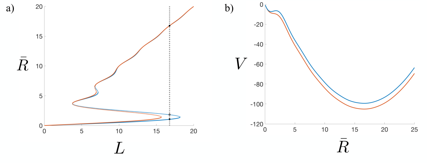
The bistable response can also be used to detect and amplify small optical signals, which we now discuss. The mechanism is illustrated in Figure 9a). We consider a value of the cooperativity $\bar{C}$ and a fixed drive strength $L$ (dashed vertical line) below but close to the bifurcation point $L_{+}$. If the system resides in the lower stable state where $\bar{R}\sim 1$, a sufficiently large negative change in the cooperativity to $C(\tau)=\bar{C}-c(\tau)$ can decrease the critical drive strength $L_{+}$ such that $L>L_{+}$. This will force the mechanical amplitude to grow to $\bar{R}\sim L$, since the lower stable state vanishes. If the size and duration of the pulse $c(\tau)$ was sufficiently large, the system will eventually reside in the upper stable state even when the cooperativity returns to $\bar{C}$. This means that a small, negative change in optical power can lead to a large permanent change in the mechanical amplitude and thereby strongly influence the optical response of the cavity.

We now quantify the optical amplification in this scheme. The average input amplitude is defined as $\bar{a}_{\mathrm{in}}(\Omega)=\Omega/\sqrt{\kappa}$, which means that the square of the input amplitude is the incoming photon flux to the cavity. We consider first a constant change in cooperativity $C=\bar{C}-\Delta C$ caused by a change in the optical drive strength to $\Omega=\bar{\Omega}-\Delta\Omega$, such that $\Delta C/\bar{C}\approx 2\Delta\Omega/\bar{\Omega}$ for $\Delta\Omega/\Omega\ll 1$. We denote the average output amplitude at the cavity resonance frequency $\bar{a}_{0,\mathrm{out}}(\Omega)=\sqrt{\kappa}\,a_{0}(\Omega)$, where $a_{0}$ is defined according to Equation (7). The amplifier power gain is then defined by

$${\cal G}_{o}=\left|\frac{\bar{a}_{0,\mathrm{out,l}}(\bar{\Omega})-\bar{a}_{0,\mathrm{out,u}}(\bar{\Omega})}{\bar{a}_{\mathrm{in}}(\bar{\Omega}+\Delta\Omega)-\bar{a}_{\mathrm{in}}(\bar{\Omega})}\right|^{2}$$

(50)

Inserting for $a_{0}$ gives

$${\cal G}_{o}=\left(\frac{\Omega}{\Delta\Omega}\right)^{2}\left[\sum_{n}\kappa\chi_{n}\left(J_{n}(\bar{R}_{\mathrm{st,l}})J_{n+1}(\bar{R}_{\mathrm{st,l}})-J_{n}(\bar{R}_{\mathrm{st,u}})J_{n+1}(\bar{R}_{\mathrm{st,u}})\right)\right]^{2}$$

(51)

In the resolved sideband regime, for large cooperativity and $L$ close to $L_{+}$, we have $\bar{R}_{\mathrm{st,l}}\sim 1$ and $J_{n}(\bar{R}_{\mathrm{st,u}})\approx 0$, which gives

$${\cal G}_{o}\sim{\cal O}\left(\frac{\bar{C}}{\Delta C}\right)^{2}\ .$$

(52)

We see that a large gain can be realized for a sufficiently small cooperativity change $\Delta C/\bar{C}$. However, it is again the thermal or quantum noise that limits how small $\Delta C$ can be.

To demonstrate the optical latch amplification mechanism, we have again solved the classical, stochastic equation (42) numerically as in Section III. For simplicity, we model the cooperativity change as a Gaussian,

$$c(\tau)=\Delta C\times\mathrm{exp}\left[-\frac{(\tau-\bar{\tau})^{2}}{2(\Delta\tau)^{2}}\right]\ ,$$

(53)

with a maximum value $\Delta C$, centered at time $\bar{\tau}$, and temporal width $\Delta\tau$. We have again chosen a value of $L$ such that noise-induced switching is negligible for the unperturbed cooperaticity $\bar{C}$. The simulation results are similar to the ones in Section III, showing that the probability of switching from the lower to the upper stable state rises with increasing $\Delta C$. In Figure 9, we show the switching probability as a function of $\Delta C/\bar{C}$ for two different pulse durations. For a long pulse $\Delta\tau=10$ which the system can follow adiabatically, we find that the probability of switching is close to unity for $\Delta C/\bar{C}\gtrsim 5\cdot 10^{-4}$. For a shorter pulse $\Delta\tau=0.1$, we find that $\Delta C/\bar{C}\gtrsim 1.5\cdot 10^{-2}$ is necessary for a large probability of switching due to the pulse.

We will now briefly consider how the bistable behaviour can also be used to store binary data. The middle curve in Figure 11, shown in red, depicts the mechanical steady-state amplitude $\bar{R}$ as a function of drive strength $L$ for a cooperativity $C=1.850$, which is just above the critical cooperativity $C_{\mathrm{crit}}\approx 1.82$. Let us assume that $L$ is fixed at the position of the vertical dotted line. If the system resides in the lower stable state, we can switch to the upper stable state by changing the cooperativity to $C_{\uparrow}<C$ by slightly adjusting the optical power. The value $C_{\uparrow}$ is chosen such that only the upper stable state remains for the fixed value of $L$, as shown by the upper (blue) curve in Figure 11. Once the amplitude has increased beyond a certain value, the system will end up in the upper stable state even when the cooperativity is returned to $C$. In other words, the system can be switched from the lower to the upper stable state by a small temporary decrease in optical input power. Conversely, if one wants to switch from the upper to the lower state, this can be done by a slight increase in optical input power resulting in a temporary increase in cooperativity to $C_{\downarrow}$ for which there is no upper stable state - see the lower (yellow) curve in Figure 11. This means that the mechanical memory can be switched back and forth simply by optical means.

This discussion is based on the system adiabatically following the change in cooperativity, which assumes that the optical pulses are much longer than the intrinsic mechanical decay time. As with the amplification scheme, it is possible to switch between the lower and the upper state with shorter pulses, but the reponse time of the memory, i.e., the time it takes to reach the other stable state, is set by the mechanical decay time.

We now define the model which includes two degenerate cavity modes $a_{1}$ and $a_{2}$ that are coupled by photon tunneling at a rate $J$ and that both couple to the same mechanical mode with the same rate, but opposite signs:

$\displaystyle H=\hbar J\left(a_{1}^{\dagger}a_{2}+a_{2}^{\dagger}a_{1}\right)+\hbar g_{0}\,x\left(a_{1}^{\dagger}a_{1}-a_{2}^{\dagger}a_{2}\right)+\hbar\omega_{m}c^{\dagger}c\ .$

(54)

We note that the model (55) can be realized on several experimental platforms, for example the membrane-in-the-middle setup [41, 39] or optomechanical crystals [42, 38]. For a tunneling rate $J$ exceeding the cavity linewidths, it is convenient to switch to a basis $a_{+}$ and $a_{-}$ in which the photon sector is diagonal. The modes $a_{+}$ and $a_{-}$ will then differ in frequency by $2J$. We assume that $J$ can be controlled such that this frequency difference matches the mechanical frequency $\omega_{m}$. The Hamiltonian can then be written

$\displaystyle H=\hbar g_{0}\left(\tilde{a}_{+}^{\dagger}\tilde{a}_{-}\tilde{c}+\tilde{a}_{-}^{\dagger}\tilde{a}_{+}\tilde{c}^{\dagger}\right)\ ,$

(55)

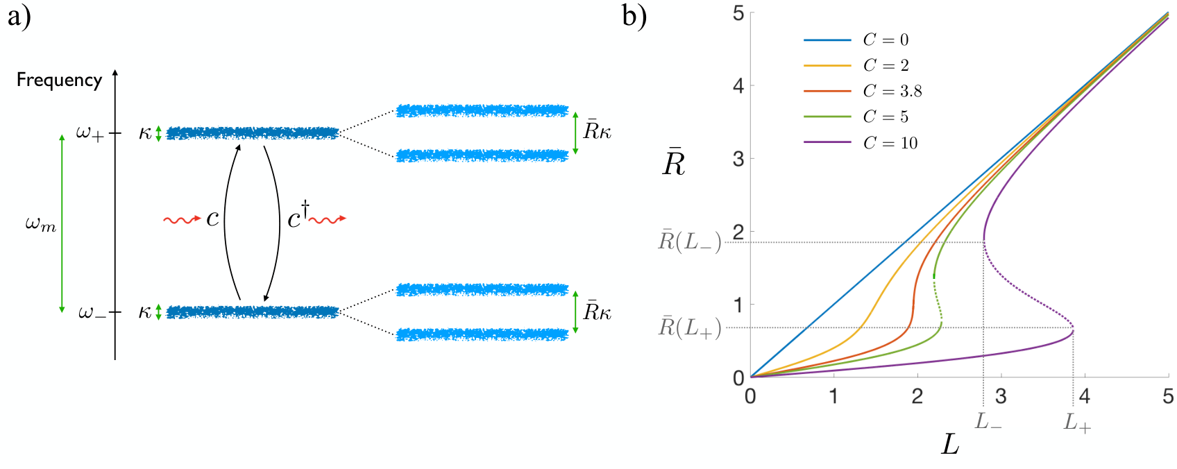
where the operators refer to frames rotating at the modes’ respective resonance frequencies. The terms in the Hamiltonian describe processes where photons can scatter between the two cavity modes, either by creation or annihilation of a phonon. These processes are depicted in Figure 12a).

We have applied the rotating wave approximation by neglecting processes such as $a_{+}^{\dagger}a_{-}c^{\dagger}$ that, at least from a naive viewpoint, do not conserve energy. We will comment on the validity of this approximation below.

References

- [1] D. McClelland, N. Mavalvala, Y. Chen, and R. Schnabel, Laser & Photonics Reviews 5, 677 (2011).
- [2] M. Metcalfe, Applied Physics Reviews 1, 031105 (2014).
- [3] A. P. Reed, K. H. Mayer, J. D. Teufel, L. D. Burkhart, W. Pfaff, M. Reagor, L. Sletten, X. Ma, R. J. Schoelkopf, E. Knill, and K. W. Lehnert, Nat. Phys. 13, 1163 (2017).
- [4] M. Arndt and K. Hornberger, Nat. Phys 10, 271 (2014).
- [5] J. D. Teufel, T. Donner, D. Li, J. W. Harlow, M. S. Allman, K. Cicak, A. J. Sirois, J. D. Whittaker, K. W. Lehnert, and R. W. Simmonds, Nature 475, 359 (2011).
- [6] J. Chan, T. P. M. Alegre, A. H. Safavi-Naeini, J. T. Hill, A. Krause, S. Gröblacher, M. Aspelmeyer, and O. Painter, Nature 478, 89 (2011).
- [7] R. Riedinger, A. Wallucks, I. Marinkovic, C. Löschnauer, M. Aspelmeyer, S. Hong, and S. Gröblacher, Nature 556, 473 (2018).
- [8] C. F. Ockeloen-Korppi, E. Damskagg, J.-M. Pirkkalainen, A. A. Clerk, F. Massel, M. J. Woolley, and M. A. Sillanpaa, Nature 556, 478 (2018).
- [9] E. Verhagen and A. Alú, Nat. Phys. 13, 922 (2017).
- [10] V. B. Braginsky, S. E. Strigin, and S. P. Vyatchanin, Phys. Lett. A 287, 331 (2001).
- [11] T. Carmon, H. Rokhsari, L. Yang, T. J. Kippenberg, and K. J. Vahala, Phys. Rev. Lett. 94, 223902 (2005).
- [12] T. J. Kippenberg, H. Rokhsari, T. Carmon, A. Scherer, and K. J. Vahala, Phys. Rev. Lett. 95, 033901 (2005).
- [13] F. Marquardt, J. G. E. Harris, and S. M. Girvin, Phys. Rev. Lett. 96, 103901 (2006).
- [14] A. G. Krause, J. T. Hill, M. Ludwig, A. H. Safavi-Naeini, J. Chan, F. Marquardt, and O. Painter, Phys. Rev. Lett. 115, 233601 (2015).
- [15] F. M. Buters, H. J. Eerkens, K. Heeck, M. J. Weaver, B. Pepper, S. de Man, and D. Bouwmeester, Phys. Rev. A 92, 013811 (2015).
- [16] H. M. Gibbs, S. L. McCall, and T. N. C. Venkatesan, Phys. Rev. Lett. 36, 1135 (1976).
- [17] I. Siddiqi, R. Vijay, F. Pierre, C. M. Wilson, M. Metcalfe, C. Rigetti, L. Frunzio, and M. H. Devoret, Phys. Rev. Lett. 93, 207002 (2004).
- [18] I. Siddiqi, R. Vijay, F. Pierre, C. M. Wilson, L. Frunzio, M. Metcalfe, C. Rigetti, R. J. Schoelkopf, M. H. Devoret, D. Vion, and D. Esteve, Phys. Rev. Lett. 94, 027005 (2005).
- [19] M. I. Dykman and M. A. Krivoglaz, Zh. Eksp. Teor. Fi. 77, 60 (1980), [Sov. Phys. JETP 50, 30 (1979)].
- [20] J. S. Aldridge and A. N. Cleland, Phys. Rev. Lett. 94, 156403 (2005).
- [21] R. B. Karabalin, R. Lifshitz, M. C. Cross, M. H. Matheny, S. C. Masmanidis, and M. L. Roukes, Phys. Rev. Lett. 106, 094102 (2011).
- [22] X. Dong, M. Dykman, and H. Chan, Nat. Comm. 9, 3241 (2018).
- [23] A. Dorsel, J. D. McCullen, P. Meystre, E. Vignes, and H. Walther, Phys. Rev. Lett. 51, 1550 (1983).
- [24] M. Bagheri, M. Poot, M. Li, W. P. H. Pernice, and H. X. Tang, Nature Nanotech. 6, 726 (2011).
- [25] H. Xu, U. Kemiktarak, J. Fan, S. Ragole, J. Lawall, and J. M. Taylor, Nat. Comm. 8, 14481 (2017).
- [26] M. I. Dykman, Phys. Rev. E 75, 011101 (2007).
- [27] C. W. Gardiner and M. J. Collett, Phys. Rev. A 31, 3761 (1985).
- [28] A. A. Clerk, M. H. Devoret, S. M. Girvin, F. Marquardt, and R. J. Schoelkopf, Rev. Mod. Phys. 82, 1155 (2010).
- [29] V. B. Braginsky and S. P. Vyatchanin, Phys. Lett. A 293, 228 (2002).
- [30] F. Marquardt, J. P. Chen, A. A. Clerk, and S. M. Girvin, Phys. Rev. Lett. 99, 093902 (2007).
- [31] I. Wilson-Rae, N. Nooshi, W. Zwerger, and T. J. Kippenberg, Phys. Rev. Lett. 99, 093901 (2007).
- [32] A. Kronwald, F. Marquardt, and A. A. Clerk, Phys. Rev. A 88, 063833 (2013).
- [33] H. Kramers, Physica (Utrecht) 7, 284 (1940).
- [34] J. Langer, Annals of Physics 54, 258 (1969).
- [35] P. Hänggi, Journal of Statistical Physics 42, 105 (1986).
- [36] P. E. Kloeden and E. Platen, Numerical Solution to Stochastic Differential Equations (Springer, New York, 1999).
- [37] G. Heinrich, J. G. E. Harris, and F. Marquardt, Phys. Rev. A 81, 011801 (2010).
- [38] A. H. Safavi-Naeini and O. Painter, New Journal of Physics 13, 013017 (2011).
- [39] M. Ludwig, A. H. Safavi-Naeini, O. Painter, and F. Marquardt, Phys. Rev. Lett. 109, 063601 (2012).
- [40] K. Stannigel, P. Komar, S. J. M. Habraken, S. D. Bennett, M. D. Lukin, P. Zoller, and P. Rabl, Phys. Rev. Lett. 109, 013603 (2012).
- [41] J. D. Thompson, B. M. Zwickl, A. M. Jayich, F. Marquardt, S. M. Girvin, and J. G. E. Harris, Nature 452, 72 (2008).
- [42] M. Eichenfield, J. Chan, R. M. Camacho, K. J. Vahala, and O. Painter, Nature 462, 78 (2009).
- [43] S. H. Autler and C. H. Townes, Phys. Rev. 100, 703 (1955).