Numerical scheme for simulation of transient flows of non-Newtonian fluids characterised by a non-monotone relation between the symmetric part of the velocity gradient and the Cauchy stress tensorThanks: This research was supported by ERC-CZ project LL1202 funded by Ministry of Education, Youth and Sports of the Czech Republic. Josef Málek and Vít Průša acknowledge the support of the Czech Science Foundation project 18-12719S. Adam Janečka acknowledges the support of project 260449/2018 “Student research in the field of physics didactics and mathematical and computer modelling”

The response of non-Newtonian fluids is mathematically described in terms of a constitutive relation that links the Cauchy stress tensor $\mathbb{T}$ and kinematical variables such as the symmetric part of the velocity gradient $\mathbb{D}$. In the case of incompressible non-Newtonian fluids, the stress is decomposed to the traceless part ${\mathbb{T}}_{\delta}=_{\mathrm{def}}\mathbb{T}-\frac{1}{3}\Tr\mathbb{T}$ and the spherical part $-p\mathbb{I}$,

and a specific non-Newtonian fluid is usually characterised by an explicit constitutive equation of the type

where ${\mathfrak{f}}$ is a monotone tensorial function. However, adequate description of the response of various non-Newtonian fluids requires one to consider non-monotone tensorial functions ${\mathfrak{f}}$ in (1.2), see for example David and Filip (2004) and Galindo-Rosales et al. (2011). The non-monotone response also seems to be crucial in modelling complex non-Newtonian phenomena such as shear banding, see Fardin et al. (2012) or Divoux et al. (2016).

More importantly, several fluids have been reported to exhibit the behaviour that do not fit into the framework (1.2), but one can still formulate the constitutive relation as an algebraic relation between ${\mathbb{T}}_{\delta}$ and $\mathbb{D}$. In particular, constitutive relations for these fluids can take the form

where ${\mathfrak{g}}$ can be again a non-monotone function. Moreover, one can also think about general implicit relations of the type

where ${\mathfrak{h}}$ is a tensorial function. One of the very first observations of the fluid response that could be characterised by (1.3) is due to Boltenhagen et al. (1997), and the amount of experimental or theoretical works concerning the non-monotonous response of the type (1.3) has been growing since then, see for example Perlácová and Průša (2015), Janečka and Průša (2015), Rajagopal and Saccomandi (2016) or Janečka and Pavelka (2018) for further references.

Typically, the non-monotone behaviour of ${\mathfrak{g}}$ exhibits itself as an S-shaped curve in shear stress/shear rate plot, see Figure 1. If one wants to avoid “multivalued” relations of the type (1.2), then is clear that the non-monotonicity of ${\mathfrak{g}}$ prevents one to invert (1.3), and write constitutive relation (1.3) in the form (1.2). Consequently, the class of fluids with constitutive relation of the type (1.3) substantially differs from the class of constitutive relations of the type (1.2).

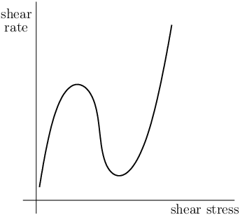
Flows of fluids with a non-monotone constitutive relation of the type (1.3) have been to our best knowledge investigated only in special geometries, where the corresponding system of governing equations reduces to a system of ordinary differential equations, see for example Málek et al. (2010), Le Roux and Rajagopal (2013), Narayan and Rajagopal (2013), Srinivasan and Karra (2015), Mohankumar et al. (2015) and Fusi and Farina (2017). However, if one needs to investigate flows in more complex geometries, a suitable numerical scheme for solution of transient flow problems must be developed. Our aim is to address this issue.

A particular constitutive relation that falls into the class (1.3) is the constitutive relation¹¹ 1 The norm of a tensorial quantity ${\mathbb{A}}$ is defined as the standard Frobenius norm, $\left|{\mathbb{A}}\right|=_{\mathrm{def}}\left(\Tr\left({\mathbb{A}}{\mathbb{A}}^{\top}\right))\right)^{\frac{1}{2}}$.

that has been introduced by Le Roux and Rajagopal (2013), see also Málek et al. (2010). Symbols $\alpha$, $\beta$ denote positive constants, $\gamma$ is a nonnegative constant, and the exponent $s$ is a constant. If $s<-\frac{1}{2}$, then one can obtain, in general, a non-monotone response, see Figure 2a, hence one is mainly interested in these values of the exponent $s$. (See Le Roux and Rajagopal (2013, Lemma 2.1) for a quantification of parameters range that lead to a non-monotone response.) Clearly, the development of a numerical scheme dealing with the simple constitutive relation (1.5) for $s<-\frac{1}{2}$ is a necessary step in the development of numerical schemes for more complex constitutive relations that belong into the class (1.3).

The corresponding system of governing equations for an incompressible non-Newtonian fluid specified by constitutive relation (1.5) reads

where $\rho$ denotes the constant density, $\bm{v}$ the Eulerian velocity field, $\bm{b}$ the external body forces, and $\frac{\mathrm{d}{}}{\mathrm{d}{t}}$ stands for the material time derivative. The first difficulty in solving (1.6) for $s<-\frac{1}{2}$ is the fact that one can not, in general, invert (1.6c) and express ${\mathbb{T}}_{\delta}$ as a function of $\mathbb{D}$. (The constitutive curve is non-monotone provided that $s<-\frac{1}{2}$, and that the other parameter values satisfy inequality $\frac{\gamma}{\alpha}<2\left(\frac{2s-2}{2s+1}\right)^{s-1}$, see Le Roux and Rajagopal (2013).) Consequently, system (1.6) can not be, in general, formulated as a system for the pressure-velocity pair $(p,\bm{v})$. However, this is just a matter of a reformulation of the problem as a problem for the pressure-velocity-stress triple $(p,\bm{v},{\mathbb{T}}_{\delta})$.

The key conceptual difficulty is the treatment of the constitutive relation (1.6c). The reason is that (1.6c) admits for $s<-\frac{1}{2}$ multiple values of ${\mathbb{T}}_{\delta}$ to be associated with the same value of the symmetric part of the velocity gradient $\mathbb{D}$. In what follows we focus exclusively on this most interesting case, that is we consider only $s<-\frac{1}{2}$.

Unfortunately, the multiplicity issue prevents one from using most of the already available analytical and numerical results regarding initial and boundary value problems for systems of the type

where ${\mathfrak{f}}({\mathbb{T}}_{\delta},\mathbb{D})$ is an implicit function. The available results, see Bulíček et al. (2009); Bulíček et al. (2012); Bulíček et al. (2012) and also Maringová and Žabenský (2018) for the proof of long-time and large-data existence of weak solution to (1.7) and similar systems, and Stebel (2016), Diening et al. (2013) and Süli and Tscherpel (2018) for the results concerning the discretised counterparts of (1.7), are based on the fact that the equation ${\mathfrak{f}}({\mathbb{T}}_{\delta},\mathbb{D})=\mathbb{0}$ defines a maximal monotone graph. Although the maximal monotone graph defined by ${\mathfrak{f}}$ can be possibly multivalued, such as in the case of Bingham fluid, see Bulíček et al. (2012) and Hron et al. (2017), systems of the type (1.6) with non-monotone response, that is (1.6c) with $s<-\frac{1}{2}$, are not covered by the otherwise very general theory by Bulíček et al. (2009); Bulíček et al. (2012).

The numerical scheme for solution of (1.6) introduced below represents the first attempt to study systems of type (1.6). The proposed scheme does not fully answer the question on the existence of a solution to (1.6), yet an important step is made. Namely, a discrete finite-dimensional nonlinear system that arises in the time-stepping of system (1.6) is shown to be solvable.

The work is organized as follows. In Section 2 we reformulate system (1.6) as a nonlinear system for the pressure-velocity-apparent viscosity triple $(p,\bm{v},\mu)$. The reformulation is the key step in the derivation of the numerical scheme. The tensorial constitutive relation (1.5) is effectively replaced by an implicit relation for a scalar quantity—the apparent viscosity—and the arising system shares some similarities with the standard Navier–Stokes system. Moreover, the apparent viscosity function introduced by this reformulation is monotone and bounded which allows one to obtain a priori estimates.

Then, in Section 3 we describe a numerical scheme for the solution of the governing equations, and we show that there exists a solution to the discretised counterpart of the governing equations.

In order to study the dynamical behaviour implied by the non-monotone constitutive relations, we introduce, see Section 4, a reduced version of the problem. In the reduced problem we neglect the contributions from other effects like pressure (incompressibility) or convection, and we focus solely on the constitutive relation. (Note that the reduced problem can be seen as a heat conduction problem with non-monotonous heat flux versus temperature gradient constitutive relation, see Janečka and Pavelka (2018) and references therein.) We introduce a variant of the proposed numerical scheme for the reduced problem, and we present several numerical experiments that document the behavior of the reduced system.

In Section 5 we move forward and we solve the full problem (1.6). Using the proposed numerical scheme we perform numerical experiments in two settings. First, we investigate the flow in the cylindrical Couette geometry, and, second, we investigate the flow in a channel with a narrowing. Finally, the conclusions of our work are stated in Section 6.

Let us consider a bounded domain $\Omega\subset\mathbb{R}^{d}$ with $(d=2,3)$. For the sake of simplicity of the discussion let us further assume that no external body force is present, $\bm{b}=\bm{0}$. Then system (1.6) reads

where the standard notation $\frac{\mathrm{d}{\bm{v}}}{\mathrm{d}{t}}=_{\mathrm{def}}\frac{\partial{\bm{v}}}{\partial{t}}+\left(\bm{v}\bullet\nabla\right)\bm{v}$, $\mathbb{D}=_{\mathrm{def}}\frac{1}{2}\left(\nabla\bm{v}+\left(\nabla\bm{v}\right)^{\top}\right)$, $\left|{\mathbb{T}}_{\delta}\right|=_{\mathrm{def}}\Tr\left({\mathbb{T}}_{\delta}{\mathbb{T}}_{\delta}^{\top}\right)^{\frac{1}{2}}$ has been used. Note that since the trace of ${\mathbb{T}}_{\delta}$ is by definition equal to zero, the constitutive relation (2.1c) in fact already enforces the incompressibility constraint (2.1a). We shall however keep (2.1a) in the system, since the constitutive relation (2.1c) will be soon reformulated. The price paid for the reformulation is that the identity (2.1a) that otherwise automatically follows from (2.1c) must be kept in the reformulated system in an explicit way.

The system is supplemented with the initial and boundary conditions in the form

(The zero Dirichlet boundary condition (2.2b) is used in mathematical analysis of the the governing equations. In the numerical simulations we use a non-zero Dirichlet boundary condition.) The aim is to find the triple $(p,\bm{v},{\mathbb{T}}_{\delta})$ such that it solves (2.1) subject to (2.2).

Introducing the apparent viscosity $\mu$ by the formula

we see that the apparent viscosity $\mu(\bm{x},t)$ can be rewritten as a function of the traceless part of the Cauchy stress tensor, that is $\mu(\bm{x},t)=\tilde{\mu}(\left|{\mathbb{T}}_{\delta}(\bm{x},t)\right|)$, where

Note that if $s<-1/2$, then the apparent viscosity $\tilde{\mu}$ introduced in (2.4) is a positive increasing and bounded function of $u$ satisfying for all $u\in[0,+\infty)$ inequalities

see Figure 2b. Further, constitutive relation (2.1c) can be rewritten as ${\mathbb{T}}_{\delta}=\tilde{\mu}(\left|{\mathbb{T}}_{\delta}\right|)\mathbb{D}$, which implies that system (2.1) can be reformulated as a system

for the triple $(p,\bm{v},\mu)$. Note that the last equation is an implicit equation for the apparent viscosity $\mu$ in terms of $\mathbb{D}$. This reformulation is a useful one, since the implicit equation is now an equation for a scalar variable, while in (2.1) the implicit equation is an equation for a tensorial variable.

At this stage, we can observe that taking the scalar product of (2.6b) with $\bm{v}$ in (2.6b) and using the incompressibility constraint (2.6a), we formally arrive to the identity

If the boundary condition reads $\left.\bm{v}\right|_{\Omega}=\bm{0}$, that is if the system is mechanically isolated, then the integration of (2.7) over $\Omega$ and the application of the Stokes theorem leads us to the formal balance of mechanical energy

In particular, (2.8)) implies that the kinetic energy is indeed dissipated. Further, due to (2.5), we see that (2.8) also implies a priori estimates analogous to that available for the standard Navier-Stokes system,

Concerning the pressure, one expects at least for spatially periodic problem or for any kind of slip conditions, see Bulíček and Málek (2016), to recover the same estimates obtained in the theory of the Navier-Stokes equations, namely

where the pressure $p$ is suitably normalised, for example via the condition $\int_{\Omega}p\,\mathrm{d}\mathrm{v}=0$.

The aim is to propose a numerical scheme that can be used in solving (2.6) by finite elements in space and finite differences in time. We exploit the fact that unlike in (2.1c) the implicit constitutive relation in (2.6) is replaced by a scalar implicit constitutive relation for the apparent viscosity.

Concerning the time discretisation, we assume a uniform partition of the time interval, $t_{n}=n\Delta t$, where $\Delta t>0$ represents a fixed time step. Moreover, since the main issue is the non-monotonicity of the constitutive relation, we for the sake of simplicity neglect the convective terms in the presentation of the numerical algorithm. However, the convective term is present in the numerical experiments reported later in Section 5.

Let ${\bm{V}}_{h}$, $P_{h}$ and $T_{h}$ be finite-dimensional spaces with bases $\left\{\bm{\phi}_{k}\right\}_{k=1}^{N_{\bm{V}}}$, $\left\{q_{k}\right\}_{k=1}^{N_{P}}$ and $\left\{t_{k}\right\}_{k=1}^{N_{T}}$ respectively, while the pair ${\bm{V}}_{h}$, $P_{h}$ satisfies the standard Babuška–Brezzi condition, see for example Brezzi and Fortin (1991). In practice, ${\bm{V}}_{h}$, $P_{h}$ and $T_{h}$ denote the finite element spaces, related to a regular triangulation $\mathcal{T}_{h}$ of the domain $\Omega$, see Section 5 for the specification of the finite lement spaces used in the numerical experiments. Let us assume that the solution at time $t_{n}$ denoted as $(\bm{v}^{n},p^{n},\mu^{n})\in\bm{V}_{h}\times P_{h}\times T_{h}$ is known, and let us compute the solution at time $t_{n+1}$ denoted as $(\bm{v}^{n+1},p^{n+1},\mu^{n+1})\in\bm{V}_{h}\times P_{h}\times T_{h}$ as a solution of the following system of nonlinear algebraic equations

that must be satisfied for all base functions $(\bar{\bm{v}},\bar{p},\bar{\mu})$ in $\bm{V}_{h}\times P_{h}\times T_{h}$. Here the symbol $\overline{\mathbb{D}}$ denotes the symmetric part of the gradient of $\bar{\bm{v}}$, $\overline{\mathbb{D}}=_{\mathrm{def}}\frac{1}{2}\left(\nabla\bar{\bm{v}}+\nabla\bar{\bm{v}}^{\top}\right)$, and the symbol $(a,b)=_{\mathrm{def}}\int_{\Omega}ab\,\mathrm{d}\mathrm{v}$ denotes the standard scalar product in the Lebesgue space $L^{2}(\Omega)$.

Since (3.1) holds for all base functions $(\bar{\bm{v}},\bar{p},\bar{\mu})$ in $\bm{V}_{h}\times P_{h}\times T_{h}$, we also know that (3.1) also holds if we set $(\bar{\bm{v}},\bar{p})=(\bm{v}^{n+1},p^{n+1})$. This helps us to recover, in the case of boundary condition $\left.\bm{v}\right|_{\Omega}=\bm{0}$, the discrete version of the balance of energy (2.8),

where the last inequality follows from the iteration of the first inequality with respect to $n$, and where $\bm{v}_{0,h}$ denotes the approximation of the initial condition (2.2a) in the space $\bm{V}_{h}$. Similarly, from (3.1c) and (2.5) we get

where $\left|\Omega\right|$ denotes the area/volume of the domain $\Omega$.

The question is whether the system of nonlinear algebraic equations has a solution. Using a standard lemma, we show that that there exists at least one solution of (3.1). The standard lemma, which is proved for example in Temam (1984, Lemma 1.4, page 164, Chapter II), states that

Now we are ready to present the proof of the existence of a solution.

In order to investigate qualitative features of models based on the implicit non-monotone constitutive relations, we present a reduced version of the system (2.6), and introduce a numerical scheme analogous to the scheme proposed in Section 3. The idea is to design a reduced model that would allow us to see the qualitative behaviour that is induced by the non-monotone constitutive relation without the unnecessary complications such as the convective nonlinearity and the incompressibility condition.

Using the proposed numerical scheme, we finally solve various initial–boundary value problems for the fluid described by the non-monotone implicit constitutive relation (1.5). The proposed numerical scheme has been implemented in FreeFem++ software, see Hecht (2012), as well as in FEniCS Project software, see Logg et al. (2012) and Alnæs et al. (2015), that are general purpose software packages for solving partial differential equations using the finite element method.

In FreeFem++ the pressure–velocity pair $(p,\bm{v})$ has been approximated by the mini-element $\mathcal{P}_{1}\times\mathcal{P}_{1}-bubble$. In FEniCS the pressure-velocity pair $(p,\bm{v})$ has been approximated by the standard lowest order Taylor–Hood elements $\left(\mathcal{P}_{1},\bm{\mathcal{P}}_{2}\right)$, where $\mathcal{P}_{k}=_{\mathrm{def}}\left\{v\in C\left(\overline{\Omega}\right):\left.v\right|_{T}\in P_{k}(T),\forall T\in\mathcal{T}_{h}\right\}$ is the Lagrange element of order $k$ and $\bm{\mathcal{P}}_{k}$ is its vectorial counterpart. For the viscosity, it is not clear how to choose the appropriate finite element function space. Since it is computed as a function of the discontinuous velocity gradient from (3.13), we have used, both in FEniCS and FreeFem++, the piecewise constant approximation $d\mathcal{P}_{0}$ as the lowest order discontinuous Lagrange element $d\mathcal{P}_{k}=_{\mathrm{def}}\left\{v\in L^{2}\left(\Omega\right):\left.v\right|_{T}\in P_{k}(T),\forall T\in\mathcal{T}_{h}\right\}$. For the temporal discretization, we have used the Crank–Nicolson method. The experimental error analysis of the proposed numerical scheme is presented elsewhere, see Málek and Tierra (2015).

A numerical scheme for simulation of transient flows of incompressible non-Newtonian fluids characterised by the non-monotone constitutive relation (1.5) has been proposed. The numerical scheme has been shown to satisfy some rudimentary properties, namely the discretised system of governing equations has been shown to posses a solution, see Section 3. Using the scheme, we have performed several numerical experiments. The experiments indicate that in the scenarios where the flow is forced by an imposed velocity field, and hence by the imposed shear-rate, then only a portion of the S-shaped curve in the Cauchy stress–symmetric part of the velocity gradient plot is actually active in the complex flows. In particular, the computed flux-affinity pairs $[{\mathbb{T}}_{\delta},\mathbb{D}]$ have been found to never occupy the decreasing part of the constitutive S-shaped curve, see Figure 2b.

References

- Alnæs et al. (2015) Alnæs, M., J. Blechta, J. Hake, A. Johansson, B. Kehlet, A. Logg, C. Richardson, J. Ring, M. Rognes, and G. Wells (2015). The FEniCS project version 1.5. Archive of Numerical Software 3(100).
- Arnold and Logg (2014) Arnold, D. N. and A. Logg (2014). Periodic table of the finite elements. SIAM News 49(9).
- Boltenhagen et al. (1997) Boltenhagen, P., Y. Hu, E. F. Matthys, and D. J. Pine (1997, Sep). Observation of bulk phase separation and coexistence in a sheared micellar solution. Phys. Rev. Lett. 79, 2359–2362.
- Brezzi and Fortin (1991) Brezzi, F. and M. Fortin (1991). Mixed and hybrid finite element methods, Volume 15 of Springer Series in Computational Mathematics. New York: Springer-Verlag.
- Bulíček et al. (2012) Bulíček, M., P. Gwiazda, J. Málek, K. R. Rajagopal, and A. Świerczewska-Gwiazda (2012). On flows of fluids described by an implicit constitutive equation characterized by a maximal monotone graph. In Mathematical aspects of fluid mechanics, Volume 402 of London Math. Soc. Lecture Note Ser., pp. 23–51. Cambridge Univ. Press, Cambridge.
- Bulíček et al. (2009) Bulíček, M., P. Gwiazda, J. Málek, and A. Świerczewska-Gwiazda (2009). On steady flows of incompressible fluids with implicit power-law-like rheology. Adv. Calc. Var. 2(2), 109–136.
- Bulíček et al. (2012) Bulíček, M., P. Gwiazda, J. Málek, and A. Świerczewska-Gwiazda (2012). On unsteady flows of implicitly constituted incompressible fluids. SIAM J. Math. Anal. 44(4), 2756–2801.
- Bulíček and Málek (2016) Bulíček, M. and J. Málek (2016). On unsteady internal flows of Bingham fluids subject to threshold slip on the impermeable boundary. In H. Amann, Y. Giga, H. Kozono, H. Okamoto, and M. Yamazaki (Eds.), Recent Developments of Mathematical Fluid Mechanics, Advances in Mathematical Fluid Mechanics, pp. 135–156. Basel: Birkhäuser.
- Bustamante (2009) Bustamante, R. (2009). Some topics on a new class of elastic bodies. Proc. R. Soc. A-Math. Phys. Eng. Sci. 465(2105), 1377–1392.
- Bustamante and Rajagopal (2011) Bustamante, R. and K. R. Rajagopal (2011). Solutions of some simple boundary value problems within the context of a new class of elastic materials. Int. J. Non-Linear Mech. 46(2), 376–386.
- Bustamante and Rajagopal (2013) Bustamante, R. and K. R. Rajagopal (2013). On a new class of electroelastic bodies I. Proc. R. Soc. A: Math. Phys. Eng. Sci. 469(2149).
- Bustamante and Rajagopal (2015) Bustamante, R. and K. R. Rajagopal (2015). Implicit constitutive relations for nonlinear magnetoelastic bodies. Proc. R. Soc. A: Math. Phys. Eng. Sci. 471(2175).
- Bustamante and Rajagopal (2017) Bustamante, R. and K. R. Rajagopal (2017). Implicit equations for thermoelastic bodies. Int. J. Non-Linear Mech. 92, 144–152.
- David and Filip (2004) David, J. and P. Filip (2004). Phenomenological modelling of non-monotonous shear viscosity functions. Appl. Rheol. 14(2), 82–88.
- Diening et al. (2013) Diening, L., C. Kreuzer, and E. Süli (2013). Finite element approximation of steady flows of incompressible fluids with implicit power-law-like rheology. SIAM J. Numer. Anal. 51(2), 984–1015.
- Divoux et al. (2016) Divoux, T., M. A. Fardin, S. Manneville, and S. Lerouge (2016). Shear banding of complex fluids. Annu. Rev. Fluid Mech. 48(1), 81–103.
- Donnelly (1991) Donnelly, R. J. (1991, NOV). Taylor–Couette flow: the early days. Phys. Today 44(11), 32–39.
- Fardin et al. (2012) Fardin, M. A., T. J. Ober, C. Gay, G. Gregoire, G. H. McKinley, and S. Lerouge (2012). Potential “ways of thinking” about the shear-banding phenomenon. Soft Matter 8, 910–922.
- Fardin et al. (2015) Fardin, M.-A., O. Radulescu, A. Morozov, O. Cardoso, J. Browaeys, and S. Lerouge (2015). Stress diffusion in shear banding wormlike micelles. J. Rheol. 59(6), 1335–1362.
- Fusi and Farina (2017) Fusi, L. and A. Farina (2017). Flow of a class of fluids defined via implicit constitutive equation down an inclined plane: Analysis of the quasi-steady regime. Eur. J. Mech. B Fluids 61, 200–208.
- Fusi et al. (2018) Fusi, L., A. Farina, G. Saccomandi, and K. R. Rajagopal (2018). Lubrication approximation of flows of a special class of non-Newtonian fluids defined by rate type constitutive equations. Appl. Math. Model. 60, 508–525.
- Galindo-Rosales et al. (2011) Galindo-Rosales, F. J., F. J. Rubio-Hernández, and A. Sevilla (2011). An apparent viscosity function for shear thickening fluids. J. Non-Newton. Fluid Mech. 166(5–6), 321–325.
- Gokulnath et al. (2017) Gokulnath, C., U. Saravanan, and K. R. Rajagopal (2017). Representations for implicit constitutive relations describing non-dissipative response of isotropic materials. Z. angew. Math. Phys. 68(6), 129.
- Hecht (2012) Hecht, F. (2012). New development in FreeFem++. J. Numer. Math. 20(3-4), 251–265.
- Hron et al. (2017) Hron, J., J. Málek, J. Stebel, and K. Touška (2017). A novel view on computations of steady flows of Bingham fluids using implicit constitutive relations. J. Non-Newton. Fluid Mech.. Submitted.
- Hu et al. (1998) Hu, Y. T., P. Boltenhagen, and D. J. Pine (1998). Shear thickening in low-concentration solutions of wormlike micelles. I. Direct visualization of transient behavior and phase transitions. J. Rheol. 42, 1185–1208.
- Janečka and Pavelka (2018) Janečka, A. and M. Pavelka (2018). Non-convex dissipation potentials in multiscale non-equilibrium thermodynamics. Continuum Mech. Therm..
- Janečka and Průša (2015) Janečka, A. and V. Průša (2015). Perspectives on using implicit type constitutive relations in the modelling of the behaviour of non-newtonian fluids. AIP Conference Proceedings 1662, –.
- Le Roux and Rajagopal (2013) Le Roux, C. and K. R. Rajagopal (2013). Shear flows of a new class of power-law fluids. Appl. Math. 58(2), 153–177.
- Logg et al. (2012) Logg, A., K.-A. Mardal, and G. Wells (2012). Automated solution of differential equations by the finite element method, Volume 84 of Lecture Notes in Computational Science and Engineering. Springer.
- Málek et al. (2010) Málek, J., V. Průša, and K. R. Rajagopal (2010). Generalizations of the Navier–Stokes fluid from a new perspective. Int. J. Eng. Sci. 48(12), 1907–1924.
- Málek et al. (2018) Málek, J., V. Průša, T. Skřivan, and E. Süli (2018). Thermodynamics of viscoelastic rate-type fluids with stress diffusion. Phys. Fluids 30(2), 023101.
- Málek and Tierra (2015) Málek, J. and G. Tierra (2015). Numerical approximations for unsteady flows of incompressible fluids characterised by non-monotone implicit constitutive relations. In J. M. D. Díaz Moreno, J. C. Díaz Moreno, C. García Vázquez, J. Medina Moreno, F. Ortegón Gallego, M. C. Pérez Martínez, C. V. Redondo Neble, and J. R. Rodríguez Galván (Eds.), Proceedings of the XXIV Congress on Differential Equations and Applications, XIV Congress on Applied Mathematics, Cádiz, pp. 797–802.
- Maringová and Žabenský (2018) Maringová, E. and J. Žabenský (2018). On a Navier–Stokes–Fourier-like system capturing transitions between viscous and inviscid fluid regimes and between no-slip and perfect-slip boundary conditions. Nonlinear Anal.-Real World Appl. 41(Supplement C), 152–178.
- Mohankumar et al. (2015) Mohankumar, K. V., K. Kannan, and K. R. Rajagopal (2015). Exact, approximate and numerical solutions for a variant of Stokes’ first problem for a new class of non-linear fluids. Int. J. Non-Linear Mech. 77, 41–50.
- Narayan and Rajagopal (2013) Narayan, S. P. A. and K. R. Rajagopal (2013). Unsteady flows of a class of novel generalizations of the Navier–Stokes fluid. Appl. Math. Comput. 219(19), 9935–9946.
- Perlácová and Průša (2015) Perlácová, T. and V. Průša (2015). Tensorial implicit constitutive relations in mechanics of incompressible non-Newtonian fluids. J. Non-Newton. Fluid Mech. 216, 13–21.
- Průša and Rajagopal (2012) Průša, V. and K. R. Rajagopal (2012). On implicit constitutive relations for materials with fading memory. J. Non-Newton. Fluid Mech. 181–182, 22–29.
- Rajagopal (2003) Rajagopal, K. R. (2003). On implicit constitutive theories. Appl. Math. 48(4), 279–319.
- Rajagopal (2006) Rajagopal, K. R. (2006). On implicit constitutive theories for fluids. J. Fluid Mech. 550, 243–249.
- Rajagopal and Saccomandi (2016) Rajagopal, K. R. and G. Saccomandi (2016). A novel approach to the description of constitutive relations. Frontiers in Materials 3, 36.
- Srinivasan and Karra (2015) Srinivasan, S. and S. Karra (2015). Flow of ”stress power-law” fluids between parallel rotating discs with distinct axes. Int. J. Non-Linear Mech. 74, 73–83.
- Stebel (2016) Stebel, J. (2016). Finite element approximation of Stokes-like systems with implicit constitutive relation. In A. Handlovičová, Z. Minarechova, and D. Ševčovič (Eds.), Proceedings of the Conference ALGORITMY, Bratislava, pp. 291–300. Publishing House of Slovak University of Technology. 19th Conference on Scientific Computing, Vysoké Tatry - Podbanské, Slovakia, September 9 - 14, 2012.
- Süli and Tscherpel (2018) Süli, E. and T. Tscherpel (2018, April). Fully discrete finite element approximation of unsteady flows of implicitly constituted incompressible fluids. ArXiv e-prints.
- Temam (1984) Temam, R. (1984). Navier-Stokes equations (Third ed.), Volume 2 of Studies in Mathematics and its Applications. Amsterdam: North-Holland. Theory and numerical analysis, With an appendix by F. Thomasset.