跳到论文正文
W Papers独立论文阅读器 arXiv:1809.04251 论文正文 计算阅读时间 · 0%
引用这篇论文根据当前论文元数据生成,正式投稿前建议核对。


License: arXiv.org perpetual non-exclusive license
arXiv:1809.04251v1 [quant-ph] 12 Sep 2018

Autonomous quantum heat engine using an electron shuttle

Behnam Tonekaboni Email: uqbtonek@uq.edu.au Affiliation: School of Mathematics and Physics, University of Queensland, Brisbane, QLD, 4072, Australia Affiliation: ARC Centre for Engineered Quantum Systems, The University of Queensland, Brisbane, QLD 4072, Australia    Brendon W. Lovett Affiliation: SUPA, School of Physics and Astronomy, University of St Andrews, St. Andrews KY16 9SS, United Kingdom    Thomas M. Stace Affiliation: School of Mathematics and Physics, University of Queensland, Brisbane, QLD, 4072, Australia Affiliation: ARC Centre for Engineered Quantum Systems, The University of Queensland, Brisbane, QLD 4072, Australia
Abstract

We propose an autonomous quantum heat engine based on the thermally driven oscillation of a single electron shuttle. The electronic degree of freedom of this device acts as an internal dynamical controller which switches the interaction of the engine with the thermal baths. We show that in addition to energy flux through the thermal baths, a flux of energy is attributed to the controller and it affects the engine power.


I Introduction

With the advancement in experimental techniques, we are able to build and control devices with truly quantum degrees of freedom. In these quantum devices, the energetics and thermodynamics of the control field become important. Thermodynamics of such quantum devices have been studied in the context of quantum heat engines and fridges [1, 2, 3], driven nano-systems [4], effect of energy transfer on quantum coherence [5, 6] and many other topics. Also a quantum heat engine has been built using a single ion [7]. The majority of these studies use an external time-dependent classical control field to switch the interaction between the working system and the heat baths. The energetic cost of these control fields is often ignored.

Formally, the external classical control field is described by a time-dependent control parameter ni∈[0,1]n_{i}\in[0,1] in the interaction Hamiltonian between the engine and baths,

Hint=n1​(t)​Hinthot⊗𝟙cold+n2​(t)​𝟙hot⊗Hintcold,H_{\mathrm{int}}=n_{1}(t)H_{\mathrm{int}}^{\mathrm{hot}}\otimes\mathbb{1}^{\mathrm{cold}}+n_{2}(t)\mathbb{1}^{\mathrm{hot}}\otimes H_{\mathrm{int}}^{\mathrm{cold}}, (1)

where 𝟙hot\mathbb{1}^{\mathrm{hot}} is the identity in Hilbert space of the hot bath and HinthotH_{\mathrm{int}}^{\mathrm{hot}} is the interaction between working system and the hot bath, similar for HintcoldH_{\mathrm{int}}^{\mathrm{cold}}.

To account for the energetic cost of the control field we develop an autonomous heat engine with a time-independent Hamiltonian, in which the controller is included in system dynamics. Autonomous heat engines have received recent attention. Frenzel et al. [8] studied a quasi-autonomous engine based on an internal quantum clock which is stabilised by external measurement. Although the interaction Hamiltonian used in [8] is time independent, the external measurement result is used in a feedback loop to intermittently reset the clock. This induces a back action on the engine, so it is not a fully autonomous system. An autonomous rotor engine was proposed [9] inspired by classical rotor engine where the state of the rotor determines the interactions and is considered as the internal clock. Neither of these papers address the energetic cost of the controller or the clock.

To fully account for the energetic cost of the controller, we develop a model of an autonomous engine, by replacing the external control field with an internal dynamical quantum controller that switches the interactions between the engine and the baths [10]. Formally we replace the control parameters in the interaction Hamiltonian with the orthonormal eigenstates of the internal dynamical controller |ni⟩\left|n_{i}\right\rangle and write

Hint=|n1⟩​⟨n1|⊗Hinthot⊗𝟙cold+|n2⟩​⟨n2|⊗𝟙hot⊗Hintcold.H_{\mathrm{int}}{=}|n_{1}\rangle\langle n_{1}|\otimes H_{\mathrm{int}}^{\mathrm{hot}}\otimes\mathbb{1}^{\mathrm{cold}}+|n_{2}\rangle\langle n_{2}|\otimes\mathbb{1}^{\mathrm{hot}}\otimes H_{\mathrm{int}}^{\mathrm{cold}}. (2)

Figure 1a shows a schematic of a thermodynamic cycle using a dynamical controller. When the controller is in the state |n1⟩\left|n_{1}\right\rangle the engine interacts with the hot bath and when it is in the state |n2⟩\left|n_{2}\right\rangle the engine interacts with the cold bath.

Refer to caption
Figure 1: a) shows thermodynamic cycle of the engine ρ\rho plus the controller |n⟩​⟨n||n\rangle\langle n| between two thermal baths, hot and cold. The state of the engine changes due to thermal operations: ρ⁡(t1)→ρ⁡(t2)\rho(t_{1})\rightarrow\rho(t_{2}) and ρ⁡(t3)→ρ⁡(t4)\rho(t_{3})\rightarrow\rho(t_{4}) while it is in contact with hot and cold bath respectively. When the state of the controller changes, |n1⟩​⟨n1|→|n2⟩​⟨n2||n_{1}\rangle\langle n_{1}|\rightarrow|n_{2}\rangle\langle n_{2}|(or reverse), engine’s interaction switches from hot to cold (or cold to hot). This switching changes the state of the engine ρ⁡(t2)→ρ⁡(t3)\rho(t_{2})\rightarrow\rho(t_{3})(or ρ⁡(t4)→ρ⁡(t5)\rho(t_{4})\rightarrow\rho(t_{5})). b) shows the diagram of the single electron shuttle heat engine. A single electron shuttle (red circle) is confined in a half-harmonic potential (dashed line), between two leads (source and drain). The leads have the same chemical potential but different temperatures, indicated by the Fermi distributions shown above them. Johnson noise from the thermal lead stochastically drives the charged island and the anharmonic potential rectifies it into a net force. The mechanical mode is coupled dissipatively to a cold bath.

A heat engine absorbs heat from a hot bath to increase the energy of the working system. In quantum thermodynamics, this process happens in a thermal operation [11, 12, 13, 14]. One condition on the thermal operation is that the pure state of any ancilla (catalyst or in our case the controller) attached to the system must be the same at the beginning and the end of the thermal operation. On the other hand, in an autonomous heat engine, the controller has its own dynamics, and stochastic fluctuations during each cycle make it difficult to unambiguously define discrete phases of thermal operations.

In this paper, we introduce a fully autonomous quantum heat engine based on the oscillation of a single-electron shuttle [15, 16], in which the charge state of the shuttle acts as the control system coupling the engine to the hot bath. In section II we describe a model for this system and define the engine and the controller. In order to identify the heat flow from the hot and the cold reservoirs, in section III we briefly describe a simpler system, a charged thermally driven oscillator, where the state of the controller is held constant. In section IV we include the dynamical controller and let it evolve during the thermal operation to see its effect on the internal energy of the engine. Also we analyse the energy flow in an unravelling of the system master equation, to derive a system of stochastic dynamic equations for the engine. In section V we numerically solve and analyse dynamics of the engine. At the end, in section VI, we calculate power of the engine in semiclassical and quantum approaches and show that quantum correlations has an important role in the engine power.

II Model

Our proposed engine is a modified version of the electromechanical shuttle studied in [16]. Figure 1b illustrates the engine, consisting of a single electron island that mechanically oscillates in a potential between two leads, shuttling an electron from the source to the drain over each cycle. In [16] the voltage bias between the leads generates an electric field that drives the charged shuttle, so that it is a microscopic electric motor. In contrast, we drive the shuttle with a thermal bias (at zero voltage bias), corresponding to a microscopic thermal engine. We set the leads to the same chemical potential while allowing them to be at finite temperatures. Johnson noise from the finite temperature leads provides a stochastic driving force.

Johnson noise is approximated as white noise with zero mean, so the time averaged force is zero. To rectify this noise into a net force, we impose a nonlinear potential. For this theoretical model we use a half-harmonic potential (shown with dashed line in Figure 1b) which is easy to analyse and provides the required nonlinearity. The energy spectrum of the half-harmonic oscillator is equally spaced with an energy gap of 2​ω2\omega, which is described by a simple Hamiltonian, Hosc=2​ω​a†​aH_{\text{osc}}=2\omega a^{\dagger}a where aa is the bosonic annihilation operator of the oscillator and satisfies [a,a†]=1[a,a^{\dagger}]=1. Although the Hamiltonian of the half-harmonic oscillator is simillar to the full-harmonic, the position and momentum operators are not the same as full-harmonic due to the asymmetry in eigen-wavefunctions which are illustrated by blue shaded area in Figure 1b (For details see Appendix B). This asymmetry provides larger ⟨x^⟩\langle\hat{\mathrm{x}}\rangle for higher energy. Therefore, when Johnson noise adds energy, the oscillator feels a rectified force to the right (For details see Appendix C).

Finally, the oscillator is coupled to a cold bosonic environment, which provides a cold bath and a sink for the work output of the engine.

In our model we assume the total Hamiltonian of the shuttle, the leads, Johnson noise and the bosonic environment is

H^\displaystyle\hat{H} =ℏ​ωI​c^†​c^\displaystyle=\hbar\omega_{I}\hat{c}^{\dagger}\hat{c} (3a)
+∑kℏωs​kb^s​k†b^s​k+ℏωd​kb^d​k†b^d​k\displaystyle+\sum_{k}\hbar\omega_{sk}\hat{b}_{sk}^{\dagger}\hat{b}_{sk}+\hbar\omega_{dk}\hat{b}_{dk}^{\dagger}\hat{b}_{dk} (3b)
+∑k[τs​kFs(x^)b^s​kc^†+H.c.]\displaystyle+\sum_{k}\left[\tau_{sk}F_{s}(\hat{\mathrm{x}})\hat{b}_{sk}\hat{c}^{\dagger}+\text{H.c.}\right] (3c)
+∑k[τd​kFd(x^)b^d​kc^†+H.c.]\displaystyle+\sum_{k}\left[\tau_{dk}F_{d}(\hat{\mathrm{x}})\hat{b}_{dk}\hat{c}^{\dagger}+\text{H.c.}\right] (3d)
+2​ℏ​ω​a^†​a^\displaystyle+2\hbar\omega\hat{a}^{\dagger}\hat{a} (3e)
−e​ξ​(t)​x^​c^†​c^\displaystyle-e\xi(t)\hat{\mathrm{x}}\hat{c}^{\dagger}\hat{c} (3f)
+∑pg(a^†d^p+a^d^p†)+∑pℏωpd^p†d^p.\displaystyle+\sum_{p}g(\hat{a}^{\dagger}\hat{d}_{p}+\hat{a}\hat{d}_{p}^{\dagger})+\sum_{p}\hbar\omega_{p}\hat{d}_{p}^{\dagger}\hat{d}_{p}. (3g)

Terms (3a) to (3d) describe dynamics of the controller. Terms (3a) is the single electron energy where ωI\omega_{I} is the electronic energy level of the shuttle. We assume the island charging energy is large so that we retain only a single electronic mode with fermionic annihilation operator c^\hat{c} which satisfies {c^,c^†}=1\{\hat{c},\hat{c}^{\dagger}\}{=}1. The Hilbert space of the electrical degree of freedom is then {|0⟩,|1⟩}\{|0\rangle,|1\rangle\}, where |ne⟩|n_{e}\rangle is the state of nen_{e} electron on the shuttle.

The Hamiltonian of the leads is given in (3b), where b^s⁡(d),k\hat{b}_{s(d),k} is fermionic annihilation operator for the source(drain) at mode kk with energy ℏ​ωs⁡(d)​k\hbar\omega_{s(d)k}. Terms (3c) and (3d) are electron tunneling terms between the leads and the shuttle. The tunneling functions Fs⁡(d)F_{s(d)} indicate the position dependency of the tunneling terms, and τs⁡(d),k\tau_{s(d),k} is the tunnelling constant between the shuttle and mode kk of the source(drain).

Expressions (3e) to (3g) describe the mechanical degree of freedom. Expression (3e) is the Hamiltonian of the oscillator in the half-harmonic potential while (3f) is the coupling between thermal (Johnson) noise ξ\xi and the shuttle position x^\hat{\mathrm{x}}. We assume ⟨ξ⁡(t)⟩noise=0\langle\xi(t)\rangle_{\text{noise}}=0 and ⟨ξ⁡(t)​ξ​(t′)⟩noise=Erms2​δ​(t−t′)\langle\xi(t)\xi(t^{\prime})\rangle_{\text{noise}}=E_{\mathrm{rms}}^{2}\delta(t-t^{\prime}), where Erms=4​kB​T​RE_{\mathrm{rms}}=4k_{B}TR is the noise amplitude with temperature TT of the source lead and RR is the lead resistance. This term can be written as −e​ξ​x^​|1⟩​⟨1|-e\xi\hat{\mathrm{x}}|1\rangle\langle 1|, which is in the form of equation (2). The shuttle couples to the thermal noise (hot bath) when an electron is on board (i.e. the electronic state is |1⟩|1\rangle), and is uncoupled when it is unoccupied (i.e. the electronic state is |0⟩|0\rangle).

The last line in the Hamiltonian, (3g), describes the interaction of the oscillator with the bosonic environment where d^p\hat{d}_{p} is the bosonic annihilation operator of mode pp with energy ℏ​ωp\hbar\omega_{p}, while gg is a coupling constant.

We obtain a master equation for the shuttle by tracing out the leads and bosonic reservoir and averaging over the noise. We define the reduceed density operator for the shuttle, following averaging over Johnson noise as ρ≡⟨TrL,B​{ρT}⟩noise\rho\equiv\langle\text{Tr}_{L,B}\{\rho_{T}\}\rangle_{\text{noise}}, where ρT\rho_{T} is the density operator of the total system. In the Born-Markov approximation [17] the master equation is (See appendix D for derivation)

ρ˙=\displaystyle\dot{\rho}= −i⁡[2​ω​a^†​a^,ρ]+γ​ℒ​[c^†​c^​x^]​ρ\displaystyle-i\left[2\omega\hat{a}^{\dagger}\hat{a},\rho\right]+\gamma\mathcal{L}[\hat{c}^{\dagger}\hat{c}\hat{\mathrm{x}}]\rho (4)
+κ⁡(n¯p+1)​ℒ​[a^]​ρ+κ​n¯p​ℒ​[a^†]​ρ\displaystyle+\kappa\left(\overline{n}_{p}+1\right)\mathcal{L}[\hat{a}]\rho+\kappa\overline{n}_{p}\mathcal{L}[\hat{a}^{\dagger}]\rho
+Γs​{fs​(ωI)​ℒ​[c^†​Fs​(x^)]​ρ+(1−fs​(ωI))​ℒ​[c^​Fs​(x^)]​ρ}\displaystyle+\Gamma_{s}\left\{f_{s}(\omega_{I})\mathcal{L}[\hat{c}^{\dagger}F_{s}(\hat{\mathrm{x}})]\rho+\left(1{-}f_{s}(\omega_{I})\right)\mathcal{L}[\hat{c}F_{s}(\hat{\mathrm{x}})]\rho\right\}
+Γd​{fd​(ωI)​ℒ​[c^†​Fd​(x^)]​ρ+(1−fd​(ωI))​ℒ​[c^​Fd​(x^)]​ρ},\displaystyle+\Gamma_{d}\left\{f_{d}(\omega_{I})\mathcal{L}[\hat{c}^{\dagger}F_{d}(\hat{\mathrm{x}})]\rho+\left(1{-}f_{d}(\omega_{I})\right)\mathcal{L}[\hat{c}F_{d}(\hat{\mathrm{x}})]\rho\right\},

where ℒ⁡[O]​ρ=O​ρ​O†−12​[O†​O​ρ+ρ​O†​O]\mathcal{L}[O]\rho=O\rho O^{\dagger}-\frac{1}{2}[O^{\dagger}O\rho+\rho O^{\dagger}O] is the Lindblad super-operator [18]. Also we use dimensionless units where ℏ=1\hbar=1.

The first two lines of equation (4) describe the dynamics of the engine. The first term gives the evolution in the half-harmonic potential while the second term is an incoherent driving term due to Johnson noise with rate γ=e2​Er​m​s2∝T2\gamma=e^{2}E^{2}_{rms}\propto T^{2}. Here we have assumed that Johnson noise is fast compared to the oscillator dynamics. As a result, the stochastic driving field appears as a dissipative term (See Appendix A and [19])11 1 In the voltage driven shuttle in [16], a time-independent electric field acts on the shuttle, thus the driving term is coherent and appears as i⁡[c^†​c^​x^,ρ]i[\hat{c}^{\dagger}\hat{c}\hat{\mathrm{x}},\rho]. This is in contrast to the dissipative term in equation (4).. The second line of the master equation is the damping due to the cold bath with the mean phonon number n¯p=1/(eω/T−1)\overline{n}_{p}=1/(e^{\omega/T}-1) and damping rate κ\kappa. The last two lines of equation (4) describe the electron tunnelling between the leads and the shuttle which controls the engine–bath coupling. The rate of tunnelling depends on the Fermi distribution, fs⁡(d)​(ωI)=1/(e(ωI−μ)/Ts⁡(d)+1)f_{s(d)}(\omega_{I})=1/(e^{(\omega_{I}-\mu)/T_{s(d)}}+1) where Ts⁡(d)T_{s(d)} is temperature of the source(drain) and μ\mu is the common chemical potential.

We choose ωI\omega_{I} slightly greater than the chemical potential of the leads. Thus at zero temperature electrons are energetically excluded from the shuttle if we neglect cotunnelling processes. At finite temperature, electrons can jump on and off the shuttle. We set the drain temperature to be small so that we can approximate fd​(ωI)≈0f_{d}(\omega_{I})\approx 0. This ensures electrons do not tunnel from the drain to the shuttle and therefore the shuttle carries an electron in each cycle from the source to the drain.

The leads are positioned so that the separation is comparable to the oscillator amplitude, therefore the tunnelling amplitude depends on the shuttle position. We model this by defining Fs​(x^)=αs​e−η​x^F_{s}(\hat{\mathrm{x}})=\alpha_{s}e^{-\eta\hat{\mathrm{x}}} and Fd​(x^)=αd​eη​x^F_{d}(\hat{\mathrm{x}})=\alpha_{d}e^{\eta\hat{\mathrm{x}}}, where η\eta is the inverse of the tunnelling length and αs=A​eη​x0\alpha_{s}{=}Ae^{\eta x_{0}} and αd=A​e−η​x0\alpha_{d}{=}Ae^{-\eta x_{0}}, where x0x_{0} is the midpoint between the source and the drain, as shown in figure 1b.

For the purpose of this paper we study the dynamics of the shuttle assuming the temperature of the cold bosonic bath is low and n¯p\overline{n}_{p} is near zero (For more general thermodynamic analysis this assumption can be lifted, this will be the subject of the future work). The master equation then becomes

ρ˙=\displaystyle\dot{\rho}= −i⁡[2​ω​a^†​a^,ρ]+γ​ℒ​[c^†​c^​x^]​ρ+κ​ℒ​[a^]​ρ\displaystyle-i\left[2\omega\hat{a}^{\dagger}\hat{a},\rho\right]+\gamma\mathcal{L}[\hat{c}^{\dagger}\hat{c}\hat{\mathrm{x}}]\rho+\kappa\mathcal{L}[\hat{a}]\rho
+Γs​{fs​(ωI)​αs2​ℒ​[c^†​e−η​x^]​ρ+(1−fs​(ωI))​αs2​ℒ​[c^​e−η​x^]​ρ}\displaystyle+\Gamma_{s}\left\{f_{s}(\omega_{I})\alpha_{s}^{2}\mathcal{L}[\hat{c}^{\dagger}e^{-\eta\hat{\mathrm{x}}}]\rho+\left(1-f_{s}(\omega_{I})\right)\alpha_{s}^{2}\mathcal{L}[\hat{c}e^{-\eta\hat{\textrm{x}}}]\rho\right\}
+Γd​αd2​ℒ​[c^​eη​x^]​ρ.\displaystyle+\Gamma_{d}\alpha_{d}^{2}\mathcal{L}[\hat{c}e^{\eta\hat{\textrm{x}}}]\rho. (5)

Since the engine is the mechanical degree of freedom of the shuttle, the energy of the working system is the energy of the oscillator E=⟨Hosc⟩=2​ω​⟨a^†​a^⟩E{=}\langle H_{\textrm{osc}}\rangle{=}2\omega\langle\hat{a}^{\dagger}\hat{a}\rangle. The rate of the change of the mechanical energy of the oscillator is

d​Ed​t=Tr​[Hosc​ρ˙].\displaystyle\frac{dE}{dt}=\text{Tr}[H_{\mathrm{osc}}\dot{\rho}]. (6)

In the following we analyse this energy rate using a fixed charge (in section III) and full dynamics with electron jumps (in section IV).

III Charged Oscillator

The charge state of the shuttle determines the Johnson noise coupling. As a prelude to studying the full dynamics, we analyze the evolution for a fixed charge state of the shuttle. By using a fixed controller state (fixed charge) we focus to the thermal operation and identify heat flow to and from the thermal baths. To model this, we set a fixed charge c^†​c^=ne\hat{c}^{\dagger}\hat{c}=n_{e} on the shuttle, and set αs,d=0\alpha_{s,d}=0. The master equation for the fixed charge shuttle is then

ρ˙=−i⁡[2​ω​a^†​a^,ρ]+γ​ne2​ℒ​[x^]​ρ+κ​ℒ​[a^]​ρ.\dot{\rho}=-i\left[2\omega\hat{a}^{\dagger}\hat{a},\rho\right]+\gamma n_{e}^{2}\mathcal{L}[\hat{\mathrm{x}}]\rho+\kappa\mathcal{L}[\hat{a}]\rho. (7)

We calculate the rate of change of energy in the oscillator, i.e. equation (6), during the thermal operation, and we find

d​Ed​t\displaystyle\frac{dE}{dt} =ω​ne2​γ2−2​ω​κ​N\displaystyle=\frac{\omega n_{e}^{2}\gamma}{2}-2\omega\kappa N (8)
≡𝒬˙H−𝒬˙C,\displaystyle\equiv\dot{\mathcal{Q}}_{\text{H}}-\dot{\mathcal{Q}}_{\text{C}}, (9)

where N=⟨a†​a⟩N=\langle a^{\dagger}a\rangle is the expectation value of phonon number. In equation (9) we have defined the heat flux from the hot bath (i.e. Johnson noise) 𝒬˙H=ω​ne2​γ2\dot{\mathcal{Q}}_{\text{H}}=\frac{\omega n_{e}^{2}\gamma}{2}, and the energy flux to the cold bath 𝒬˙C=2​ω​κ​N\dot{\mathcal{Q}}_{\text{C}}=2\omega\kappa N. When ne=1n_{e}=1, the oscillator couples to Johnson noise which causes a steady increase in the mechanical energy of the system and when ne=0n_{e}=0 the oscillator is only in contact with the bosonic cold bath. We interpret equation (9) as a thermodynamic identity of the thermal operation with a static control parameter.

IV Autonomous Engine

Equation (8) and its thermodynamic interpretation equation (9) consider only the energy flow from and to the thermal baths. They do not include power attributed to the dynamical controller (i.e. tunnelling). To account for this, we calculate energy rate, equation (6), from the full dynamical system, including the controller i.e. equation (5). We find

d​Ed​t\displaystyle\frac{dE}{dt} =ω​γ​⟨c†​c⟩22−2​ω​κ​N\displaystyle=\frac{\omega\gamma\langle c^{\dagger}c\rangle^{2}}{2}-2\omega\kappa N
+12​ω​Γs​αs2​η2​[fs​(1−⟨c†​c⟩)+(1−fs)​⟨c†​c⟩]​⟨e−2​η​x^⟩\displaystyle+\frac{1}{2}\omega\Gamma_{s}\alpha_{s}^{2}\eta^{2}\left[f_{s}(1-\langle c^{\dagger}c\rangle)+(1-f_{s})\langle c^{\dagger}c\rangle\right]\langle e^{-2\eta\hat{\mathrm{x}}}\rangle
+12​ω​Γd​αd2​η2​⟨c†​c⟩​⟨e2​η​x^⟩\displaystyle+\frac{1}{2}\omega\Gamma_{d}\alpha_{d}^{2}\eta^{2}\langle c^{\dagger}c\rangle\langle e^{2\eta\hat{\mathrm{x}}}\rangle (10)
≡𝒬˙H−𝒬˙C+E˙control.\displaystyle\equiv\dot{\mathcal{Q}}_{\text{H}}-\dot{\mathcal{Q}}_{\text{C}}+\dot{E}_{\mathrm{control}}. (11)

where E˙control\dot{E}_{\mathrm{control}} is the contribution of the controller to the energy of the engine which can be positive or negative, meaning that the controller can add or take energy from the oscillator. Thus the thermodynamic identity for the whole system must include the control power as well as the thermal operation.

To describe the stochastic evolution of the system, we unravel the master equation into a stochastic master equation (SME), using a jump process for the charge state of the shuttle. In this unravelling the controller charge state fluctuates stochastically between |0⟩|0\rangle and |1⟩|1\rangle. In an experimental setup, the SME has an interpretation as a model of continuous measurement, in which one monitors the electron jumps and thus the evolution of the controller [20]. The SME for the conditional state of the engine is

d​ρc=\displaystyle d\rho_{c}= −i⁡[2​ω​a^†​a^,ρc]​d​t+γ​ℒ​[c^†​c^​x^]​ρc​d​t+κ​ℒ​[a^]​ρc​d​t\displaystyle-i\left[2\omega\hat{a}^{\dagger}\hat{a},\rho_{c}\right]dt+\gamma\mathcal{L}[\hat{c}^{\dagger}\hat{c}\hat{\textrm{x}}]\rho_{c}dt+\kappa\mathcal{L}[\hat{a}]\rho_{c}dt (12a)
−12​d​t​{Γs​fs​(ωI)​αs2​ℋ​[c^​c^†​e−2​η​x^]​ρc+Γs​(1−fs​(ωI))​αs2​ℋ​[c^†​c^​e−2​η​x^]​ρc}−12​d​t​Γd​αd2​ℋ​[c^†​c^​e2​η​x^]​ρc\displaystyle-\frac{1}{2}dt\left\{\Gamma_{s}f_{s}(\omega_{I})\alpha_{s}^{2}\mathcal{H}[\hat{c}\hat{c}^{\dagger}e^{-2\eta\hat{\mathrm{x}}}]\rho_{c}+\Gamma_{s}(1-f_{s}(\omega_{I}))\alpha_{s}^{2}\mathcal{H}[\hat{c}^{\dagger}\hat{c}e^{-2\eta\hat{\mathrm{x}}}]\rho_{c}\right\}-\frac{1}{2}dt\penalty\ \Gamma_{d}\alpha_{d}^{2}\mathcal{H}[\hat{c}^{\dagger}\hat{c}e^{2\eta\hat{\mathrm{x}}}]\rho_{c} (12b)
+d​N+s​𝒢​[c^†​e−η​x^]​ρc+d​N−s​𝒢​[c^​e−η​x^]​ρc+d​N−d​𝒢​[c^​eη​x^]​ρc,\displaystyle+dN_{+}^{s}\mathcal{G}[\hat{c}^{\dagger}e^{-\eta\hat{\mathrm{x}}}]\rho_{c}+dN_{-}^{s}\mathcal{G}[\hat{c}e^{-\eta\hat{\mathrm{x}}}]\rho_{c}+dN_{-}^{d}\mathcal{G}[\hat{c}e^{\eta\hat{\mathrm{x}}}]\rho_{c}, (12c)

where 𝒢\mathcal{G} and ℋ\mathcal{H} are nonlinear superoperators defined by

𝒢⁡[O]​ρ\displaystyle\mathcal{G}[O]\rho =O​ρ​O†Tr​[O​ρ​O†]−ρ\displaystyle=\frac{O\rho O^{\dagger}}{\text{Tr}[O\rho O^{\dagger}]}-\rho (13)
ℋ⁡[O]​ρ\displaystyle\mathcal{H}[O]\rho =O​ρ+ρ​O†−Tr​[O​ρ+ρ​O†]​ρ.\displaystyle=O\rho+\rho O^{\dagger}-\text{Tr}[O\rho+\rho O^{\dagger}]\rho. (14)

Terms in (12a) are the same as the first line of the equation (5) while (12c) describes electron jumps on and off the shuttle with stochastic increments d​N±sdN_{\pm}^{s} and d​N−ddN_{-}^{d} which are either 00 or 11. The probabilities of these stochastic terms depend on the state of the shuttle and have the following mean values:

⟨d​N+s⟩\displaystyle\langle dN_{+}^{s}\rangle =Γs​fs​(ωI)​αs2​Tr​[c^​c^†​e−2​η​x^​ρc]​d​t\displaystyle=\Gamma_{s}f_{s}(\omega_{I})\alpha_{s}^{2}\text{Tr}[\hat{c}\hat{c}^{\dagger}e^{-2\eta\hat{\textrm{x}}}\rho_{c}]dt (15a)
⟨d​N−s⟩\displaystyle\langle dN_{-}^{s}\rangle =Γs​(1−fs​(ωI))​αs2​Tr​[c^†​c^​e−2​η​x^​ρc]​d​t\displaystyle=\Gamma_{s}(1-f_{s}(\omega_{I}))\alpha_{s}^{2}\text{Tr}[\hat{c}^{\dagger}\hat{c}e^{-2\eta\hat{\mathrm{x}}}\rho_{c}]dt (15b)
⟨d​N−d⟩\displaystyle\langle dN_{-}^{d}\rangle =Γd​αd2​Tr​[c^†​c^​e2​η​x^​ρc]​d​t.\displaystyle=\Gamma_{d}\alpha_{d}^{2}\text{Tr}[\hat{c}^{\dagger}\hat{c}e^{2\eta\hat{\mathrm{x}}}\rho_{c}]dt. (15c)

In the SME (12), the controller has two energetic effects: 1) Back action of continuous current measurement, 2) Electron jumps which switch the bath interactions. To show this we write the change in the mechanical energy of the oscillator as

d​Ec\displaystyle dE_{c} =Tr​[Hosc​d​ρc]\displaystyle=\text{Tr}[H_{\mathrm{osc}}d\rho_{c}]
=(𝒬˙H−𝒬˙C+E˙M)​d​t+d​EJ\displaystyle=(\dot{\mathcal{Q}}_{\text{H}}-\dot{\mathcal{Q}}_{\text{C}}+\dot{E}_{M})dt+dE_{J} (16)

where 𝒬˙H\dot{\mathcal{Q}}_{\text{H}} and 𝒬˙C\dot{\mathcal{Q}}_{\text{C}} are as before while E˙M​d​t=Tr​[Hosc​{expression 12b}]\dot{E}_{M}dt=\text{Tr}[H_{\mathrm{osc}}\{\text{expression }\ref{subeq:conditional_measurement}\}] describes the energy transfer due to continuous current measurement; and d​EJ=Tr​[Hosc​{expression 12c}]dE_{J}=\text{Tr}[H_{\mathrm{osc}}\{\text{expression }\ref{subeq:conditional_jump}\}] is a stochastic term due to the electron jumps on and off the shuttle.

Refer to caption
Figure 2: Shows the time evolution of the expectation value of (a) position ⟨x^⟩\langle\hat{\mathrm{x}}\rangle, (b) electron number ⟨c†​c⟩\langle c^{\dagger}c\rangle and, (c) phonon number ⟨a†​a⟩\langle a^{\dagger}a\rangle. The solid blue lines show the unconditional solution to the master equation (5). Light purple lines are 500 trajectories of conditional dynamics, equation (12), indicating the typical spread, and the black dashed line highlights a single trajectory. (d) shows the energy flux through the oscillator (blue solid line), flux due to thermodynamic reservoirs (red dotted line), and flux due to the dynamical controller E˙control\dot{E}_{\mathrm{control}} (shaded green)

V Dynamical simulations

In this section we analyze the behaviour of the engine and the effect of the controller by solving the unconditional master equation (5) and SME (12).

We use a truncated oscillator basis and find the time evolution of the matrix elements of ρ\rho in the eigenbasis of the oscillator and the electrons. Then we calculate the expectation values of the position ⟨x^⟩\langle\hat{\mathrm{x}}\rangle, the phonon number ⟨a^†​a^⟩\langle\hat{a}^{\dagger}\hat{a}\rangle and the electron number ⟨c^†​c^⟩\langle\hat{c}^{\dagger}\hat{c}\rangle. The solid blue curves in figures 2a–c show these quantities as functions of time. Figures 2a and 2b show the shuttling behaviour of the engine: when the shuttle is near to the source lead (xsource=0x_{\text{source}}=0), average number of electrons, ⟨c^†​c^⟩\langle\hat{c}^{\dagger}\hat{c}\rangle, increases and when ⟨x^⟩\langle\hat{\mathrm{x}}\rangle is near to the drain (xdrain=0.6x_{\text{drain}}=0.6) the electron number decreases. Figure 2c shows ⟨a^†​a^⟩\langle\hat{a}^{\dagger}\hat{a}\rangle and consequently mechanical energy of the engine E=2​ω​⟨a^†​a^⟩E=2\omega\langle\hat{a}^{\dagger}\hat{a}\rangle increases.

Figure 2d shows the rate of change in mechanical energy of the engine. Peaks in E˙\dot{E} match with the peaks in ⟨c^†​c^⟩\langle\hat{c}^{\dagger}\hat{c}\rangle and it confirms that the presence of an electron acts as the controller: when the shuttle is charged the heat flux to the engine is the largest. The net heat flux 𝒬˙H−𝒬˙C\dot{\mathcal{Q}}_{H}-\dot{\mathcal{Q}}_{C} to the engine is plotted as a dotted red line while the green shaded area shows the energetic cost of the control power. The magnitude of the controller effect increases while electron number increases (and the shuttle is near to the source). This is consistent with equation (10) where electron number, ⟨c†​c⟩\langle c^{\dagger}c\rangle, has an important role in E˙control\dot{E}_{\text{control}}.

A solution to the SME (12) is a quantum trajectory. The light purple lines in figures 2a-c show 500 trajectories; one is highlighted in black dashed line. The spread of trajectories indicates the stochastic variation of x^\hat{\mathrm{x}}, c^†​c^\hat{c}^{\dagger}\hat{c} and a^†​a^\hat{a}^{\dagger}\hat{a} in figure 2a-c.

Figure 3: Shows the phase space diagram of the oscillator coordinates v=⟨p^⟩/m\text{v}=\langle\hat{\mathrm{p}}\rangle/m and ⟨x^⟩\langle\hat{\mathrm{x}}\rangle. Solid blue line shows the unconditional coordinates up to t=30​πt=30\pi (i.e. 30 cycles), which is substantially longer than 1/κ=201/\kappa=20 representing the damping time scale for the unconditional dynamics. Red dots show 50 cycles of a typical stochastic trajectory from t=450​πt=450\pi to t=500​πt=500\pi, i.e. in the long time limit. This illustrates the fact that typical trajectories do not dwell near the unconditional steady state (green point).

We plot the oscillator phase space coordinates v=⟨p^⟩/Mv=\langle\hat{\mathrm{p}}\rangle/M and ⟨x^⟩\langle\hat{\mathrm{x}}\rangle, where MM is the mass of the oscillator. The solid blue line in figure 3 shows the unconditional coordinates over 50 cycles. Phase fluctuations in the cycles cause the oscillator to damp to an unconditional steady state.

In contrast, a typical trajectory in the stochastic solution to the SME does not converge to a well defined fixed point. Instead it continues to fluctuate around the unconditional fixed point, rarely dwelling near it. A representative trajectory is shown as red points in Figure 3, where we have plotted the last 50 cycles to show that the unconditional steady state is not representative of the long time stochastic dynamics; that is, stochastic fluctuations remain large in the long time dynamics.

Refer to caption
Figure 4: shows phase diagrams of typical trajectories of the oscillator for different values of γ\gamma and fixed damping rate κ=0.05\kappa=0.05. The unconditional steady states are shown by green points. The hollow and the filled squares are fixed points for uncharged, ne=0n_{e}=0, and charged, ne=1n_{e}=1, oscillator respectively. For γ=0\gamma=0 a typical trajectory fluctuates randomly around the steady state within the size of the zero point motion 1/M​ω1/\sqrt{M\omega}. As γ\gamma increases the the stochastic cycles sweep a larger area.

We expect that the swept phase space area grows as the driving strength increases. This is demonstrated in Figure 4, which shows a series of stochastic solutions to the SME (12) as the strength of the coupling to the Johnson noise increases. Clearly, the phase space region explored by the shuttle grows as the coupling (and heat flux) increases.

Refer to caption
Figure 5: shows power spectrum of oscillator position for different values of γ\gamma. The peak at ωS​R≈2.0​ω\omega_{SR}\approx 2.0\omega indicates the existence of stochastic resonance.

Discussion– Nonlinear systems subject to noise exhibit various phenomenon including stochastic limit cycle [21] and stochastic resonance [22]. Stochastic resonance (SR) in a nonlinear system occurs when a time-dependent, periodic force is amplified by noise, and arises from a the emergence of stochastic limit cycle, in which two stable attractors become coupled by the noise. Since the discovery of SR, Gang et al. [23] and others [24] showed that nonlinear systems with fixed points subject to noise can exhibit autonomous stochastic resonance (ASR) i.e. without an externally applied periodic force.

The system we consider in this paper falls into this category: the quantum shuttle has two fixed points associated to each of the charge states of the shuttle, i.e. for ne=⟨c^†​c^⟩=0n_{e}=\langle\hat{c}^{\dagger}\hat{c}\rangle=0 and ne=1n_{e}=1. The position of these fixed points is shown in Figure 4, as a hollow square for ne=0n_{e}=0 and a filled square for ne=1n_{e}=1. Further, the shuttle is driven by both Johnson noise and the stochastic fluctuations in ⟨c†​c⟩\langle c^{\dagger}c\rangle, so it is possible for an autonomous stochastic resonance to appear.

Gang et al. [23] characterise ASR phenomena by the emergence, and subsequent growth, of a peak in the power spectrum of the system dynamics as noise power increases. Following this approach, we numerically calculate the power spectrum Sx​(ω~)=|x⁡(ω~)|2S_{x}(\tilde{\omega})=|x(\tilde{\omega})|^{2} of the phase space coordinates, where x⁡(ω~)x(\tilde{\omega}) is the Fourier transform of ⟨x^​(t)⟩\langle\hat{\mathrm{x}}(t)\rangle.

Figure 5 shows Sx​(ω~)S_{x}(\tilde{\omega}) for different values of γ\gamma. At γ=0\gamma=0, the system has only one fixed point, so it fluctuates within the zero point motion. A large value of γ\gamma is associate with longer distance between the fixed points and consequently larger oscillation. The power spectrum exhibits a clear peak around ω~=2​ω\tilde{\omega}=2\omega, which grows with increasing strength of the Johnson noise, γ\gamma, and is consistent with the characterisation of ASR phenomena. We also calculate the power spectrum of velocity (Appendix E) and find it has π/2\pi/2 phase lag relative to the position, indicating a cyclic orbit in phase space.

Furthermore, in Appendix E we show phase space histograms for different trajectories over 400 cycles. The ‘crater-like’ depression in the centre of many phase space histograms is another evidence for existence of stochastic resonance.

VI Work and Power

In classical thermodynamics, the energy output of a heat engine is split into a useful part (work) and an entropic part (heat), which depend on the process (or path). In quantum machines with high fluctuation in internal energy, such a classification of work and heat is not obvious. A common approach is based on the change of the total energy d​E=Tr​[H​d​ρ+ρ​d​H]dE=\text{Tr}[Hd\rho+\rho dH], where the first term on the right hand side is heat and the second term is work [1, 2]. This approach is not suitable for an autonomous engine with a time independent Hamiltonian. Also it has been discussed in [25] that this definition of work does not have an operational meaning.

Here we define work based on its classical counterpart. The classical definition of infinitesimal mechanical work is d​𝒲=F​d​xd\mathcal{W}=Fd\mathrm{x}, where FF is the force on the work sink. Equivalently instentanous power is 𝒫=F​v\mathcal{P}=F\text{v} where v is the velocity. In quantum mechanics, force and velocity can be correlated i.e. ⟨F​v⟩≠⟨F⟩​⟨v⟩\langle F\text{v}\rangle\neq\langle F\rangle\langle\text{v}\rangle. In the following we define work and power in two different approaches: Semiclassical and fully quantum.

In semiclassical approach, we ignore quantum correlations between force and position (or velocity). The semiclassical work output during the interval τ=tf−ti\tau=t_{f}-t_{i} is

𝒲SC​(τ)=∫titf⟨F⁡(t)⟩​d​⟨x^​(t)⟩,\displaystyle\mathcal{W}_{\text{SC}}(\tau)=\int_{t_{i}}^{t_{f}}\langle F(t)\rangle d\langle\hat{\mathrm{x}}(t)\rangle, (17)

and the equivalent instantaneous power is

𝒫SC​(t)=⟨F⁡(t)⟩​⟨v^​(t)⟩,\displaystyle\mathcal{P}_{\text{SC}}(t)=\langle F(t)\rangle\langle\hat{\text{v}}(t)\rangle, (18)

where v^​(t)=⟨p^⟩/M\hat{\text{v}}(t)=\langle\hat{\mathrm{p}}\rangle/M is the velocity of the oscillator.

For the fully quantum approach we include the correlations between FF and v^\hat{\text{v}}. Since these operators do not commute we choose the symmetrised operator, 12​(F​v^+v^​F)\frac{1}{2}(F\hat{\mathrm{v}}+\hat{\mathrm{v}}F). But this choice has a nonzero value for the ground state. To avoid a zero point power, we subtract 𝒫0=12​⟨0|F​v^+v^​F|0⟩\mathcal{P}_{0}=\frac{1}{2}\langle 0|F\hat{\mathrm{v}}+\hat{\mathrm{v}}F|0\rangle from symmetric expectation value where |0⟩|0\rangle is the gground state of the half-harmonic. We then define quantum power as

𝒫Q​(t)=12​⟨F​v^+v^​F⟩−𝒫0.\displaystyle\mathcal{P}_{\text{Q}}(t)=\frac{1}{2}\langle F\hat{\mathrm{v}}+\hat{\mathrm{v}}F\rangle-\mathcal{P}_{0}. (19)

In either approach, we need to calculate the force on the work sink. We first write Heisenberg equations of motion of phase space coordinates

d​p^d​t\displaystyle\frac{d\hat{p}}{dt} =−M​ω2​x^−κ​𝒟†​[a]​p^\displaystyle=-M\omega^{2}\hat{\mathrm{x}}-\kappa\mathcal{D}^{\dagger}[a]\hat{p}
d​x^d​t\displaystyle\frac{d\hat{\mathrm{x}}}{dt} =p^M−κ​𝒟†​[a]​x^,\displaystyle=\frac{\hat{\mathrm{p}}}{M}-\kappa\mathcal{D}^{\dagger}[a]\hat{\mathrm{x}}, (20)

where 𝒟†​[O]​A=O†​A​O−12​(O†​O​A+A​O†​O)\mathcal{D}^{\dagger}[O]A=O^{\dagger}AO-\frac{1}{2}(O^{\dagger}OA+AO^{\dagger}O) is the adjoint Lindblad super-operator.22 2 These equations are in rotating wave approximation and the dissipative terms are in both momentum and position. [26] We then compute the force from Newton’s law as follows:

M​d2​x^d​t2\displaystyle M\frac{d^{2}\hat{\mathrm{x}}}{dt^{2}} =d​p^d​t−κ​M​𝒟†​[a]​(d​xd​t)\displaystyle=\frac{d\hat{\mathrm{p}}}{dt}-\kappa M\mathcal{D}^{\dagger}[a](\frac{d\mathrm{x}}{dt})
=−M​ω2​x^−2​κ​𝒟†​[a]​p^+κ2​M​𝒟†​[a]​𝒟†​[a]​x^\displaystyle=-M\omega^{2}\hat{\mathrm{x}}-2\kappa\mathcal{D}^{\dagger}[a]\hat{p}+\kappa^{2}M\mathcal{D}^{\dagger}[a]\mathcal{D}^{\dagger}[a]\hat{\mathrm{x}}
=Fosc+FCold Bath.\displaystyle=F_{\text{osc}}+F_{\text{Cold Bath}}. (21)

Considering that the phase coordinates p^/M\hat{\mathrm{p}}/M and x^\hat{\mathrm{x}} are in dimensionless units and in the same order of magnitude (see Figure 4), the last term in equation 20 is negligible when κ≪ω\kappa\ll\omega and κ<1\kappa<1. The first term is the oscillation force due to the half-harmonic potential, Fosc=−M​ω2​x^F_{\text{osc}}=-M\omega^{2}\hat{x}. The second term is the viscous force due to interaction with the cold reservoir. We then write the working force as the negative of the bath force,

FWork=−FCold Bath=+2​κ​𝒟†​[a]​p^.F_{\text{Work}}=-F_{\text{Cold Bath}}=+2\kappa\mathcal{D}^{\dagger}[a]\hat{p}. (22)
Refer to caption
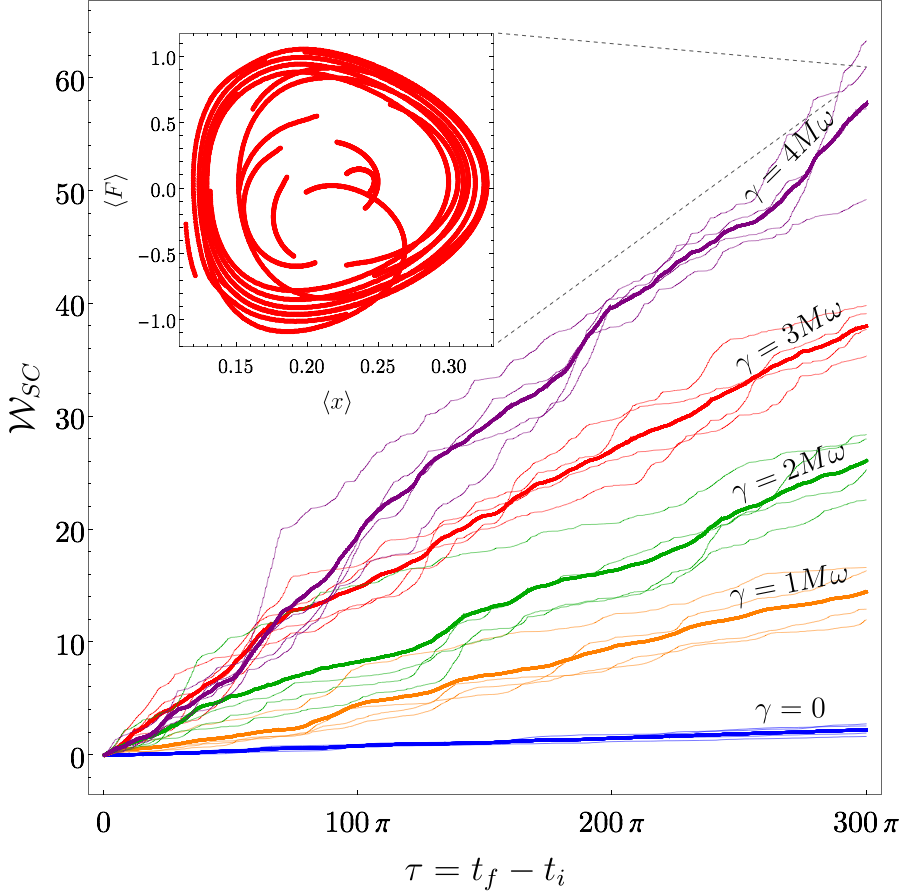
Figure 6: Semiclassical work calculated during the interval τ\tau for different values of γ\gamma. The interaction rate to the cold reservoir is chosen as κ=0.05\kappa=0.05 and initial time, tit_{i} is chosen well after transient to dynamical stationary state. Thin lines are single trajectories while thick lines are averaged over many trajectories. The inset figure shows plot of ⟨F⟩\langle F\rangle vs. ⟨x^⟩\langle\hat{\mathrm{x}}\rangle for the last 10 cycles of the trajectory with γ=4​M​ω\gamma=4M\omega. The semiclassical work for each cycle is the area enclosed in the force-position diagram.
Refer to caption
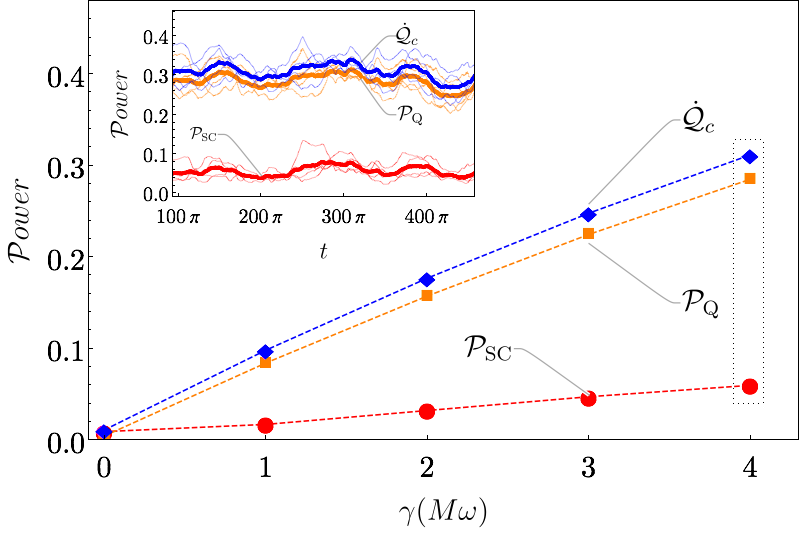
Figure 7: Shows time and trajectory averaged of 𝒫SC\mathcal{P}_{\text{SC}} (red circles), 𝒫Q\mathcal{P}_{\text{Q}} (orange squares) and 𝒬˙C\dot{\mathcal{Q}}_{\text{C}} (blue diamonds) for different value of γ\gamma with fixed κ=0.05\kappa=0.05. Dashed lines connecting the points to guide the eyes. All the quantities increase by increasing γ\gamma. Quantum power is about 5 times larger than semiclassical which indicates the importance of the force velocity correlation. Also quantum power is close to the heat flux to the cold bath. Inset plot shows 𝒫SC\mathcal{P}_{\text{SC}}, 𝒫Q\mathcal{P}_{\text{Q}} and 𝒬˙C\dot{\mathcal{Q}}_{\text{C}} for γ=4​M​ω\gamma=4M\omega as functions of time.

We use equations (17) and (22) to calculate semiclassical work for different quantum trajectories of the engine. Figure 6 shows 𝒲SC\mathcal{W}_{\text{SC}} for different value of γ\gamma. We have chosen tit_{i} well after all transitions to the dynamical steady state (i.e. system dynamics is independent from the initial state). Thin lines are 𝒲SC\mathcal{W}_{\text{SC}} for single trajectories while thick lines are averaged over trajectories. The inset plot shows the force-position diagram for the last 10 cycles of a single trajectory with γ=4​M​ω\gamma=4M\omega. The semiclassical work is the cumulative area enclosed by each cycle of this plot. The work done on the cold reservoir increases linearly (on average) which indicates a constant average power. Red circles in Figure 7 show the averaged semiclassical power. As we expect this power increases with larger γ∝THot2\gamma\propto T_{\text{Hot}}^{2}.

We also calculate power using equation (19) to include quantum correlations. Orange squares in Figure 7 shows 𝒫Q\mathcal{P}_{\text{Q}} (averaged over time and over trajectories) for different values of γ\gamma. We see that 𝒫Q\mathcal{P}_{\text{Q}} (orange squares) are about 5 times larger than 𝒫SC\mathcal{P}_{\text{SC}} (red circles). The discrepancy between the calculated semiclassical power output, and the fully correlated power output indicates that quantum correlations in the shuttle are significant

Since the cold bosonic reservoir is at zero temperature, we suspect that all the transferred energy into it, is attributable as “work”. To investigate this, we compare 𝒫SC\mathcal{P}_{\text{SC}} and 𝒫Q\mathcal{P}_{\text{Q}} to 𝒬˙C\dot{\mathcal{Q}}_{\text{C}} (blue diamonds in Figure 7) and we found that quantum power 𝒫Q\mathcal{P}_{\text{Q}} is close to 𝒬˙C\dot{\mathcal{Q}}_{\text{C}}. The small difference between 𝒫Q\mathcal{P}_{\text{Q}} and 𝒬˙C\dot{\mathcal{Q}}_{\text{C}} is approximately constant. This is shown in the inset plot in Figure 7 which compares time dependent 𝒫SC​(t)\mathcal{P}_{\text{SC}}(t),𝒫Q​(t)\mathcal{P}_{\text{Q}}(t) and 𝒬˙C​(t)\dot{\mathcal{Q}}_{C}(t) for γ=4​M​ω\gamma=4M\omega. This difference is a computational error due to truncation in oscillator energy basis which is more significant in the momentum operator of half-harmonic oscillator that is used to calculate FWorkF_{\text{Work}}.

The power is affected by the controller implicitly. It can be understood by considering that 𝒫Q≃𝒬˙C\mathcal{P}_{\text{Q}}\simeq\dot{\mathcal{Q}}_{\text{C}} and 𝒬˙C\dot{\mathcal{Q}}_{\text{C}} is proportional to phonon number. Since phonon number is affected by the controller, 𝒫Q\mathcal{P}_{\text{Q}} is affected too.

Our definitions of power were based on the damping of a classical oscillator and we adopted a zero temperature bosonic reservoir as both the cold bath and the work sink. Discriminating heat from work may be done by coupling the engine to a model of a quantum battery that stores the work output as internal energy. This will be the subject of future work.

To conclude, we have developed an autonomous heat engine based on the oscillation of a single electron shuttle. In this system the mechanical degree of freedom is the engine and the electric degree of freedom is the controller. We showed that the controller has an energetic cost to the engine power. We also defined both semiclassical and quantum power, and showed that quantum correlation between force and velocity is significant.

Acknowledgment

We would like to thank R. Kosloff, A. Nazir, J. Combes and C. Muller, K. Modi, F. Pollock and G. J. Milburn for useful discussions. This work was supported by the Australian Research Council Centre of Excellence for Engineered Quantum Systems (Grant No. CE 110001013).

References

  • [1] Ronnie Kosloff, “A quantum mechanical open system as a model of a heat engine,” The Journal of Chemical Physics 80, 1625–1631 (1984), http://dx.doi.org/10.1063/1.446862 .
  • [2] Robert Alicki, “The quantum open system as a model of the heat engine,” Journal of Physics A: Mathematical and General 12, L103 (1979).
  • [3] Ronnie Kosloff and Amikam Levy, “Quantum heat engines and refrigerators: Continuous devices,” Annual Review of Physical Chemistry 65, 365–393 (2014), pMID: 24689798, https://doi.org/10.1146/annurev-physchem-040513-103724 .
  • [4] Kay Brandner, Keiji Saito, and Udo Seifert, “Thermodynamics of micro- and nano-systems driven by periodic temperature variations,” Phys. Rev. X 5, 031019 (2015).
  • [5] Marlan O Scully, M Suhail Zubairy, Girish S Agarwal, and Herbert Walther, “Extracting work from a single heat bath via vanishing quantum coherence,” Science 299, 862–864 (2003).
  • [6] Marlan O Scully, Kimberly R Chapin, Konstantin E Dorfman, Moochan Barnabas Kim, and Anatoly Svidzinsky, “Quantum heat engine power can be increased by noise-induced coherence,” Proceedings of the National Academy of Sciences 108, 15097–15100 (2011).
  • [7] Johannes Roßnagel, Samuel T. Dawkins, Karl N. Tolazzi, Obinna Abah, Eric Lutz, Ferdinand Schmidt-Kaler, and Kilian Singer, “A single-atom heat engine,” Science 352, 325–329 (2016), http://science.sciencemag.org/content/352/6283/325.full.pdf .
  • [8] Max F Frenzel, David Jennings, and Terry Rudolph, “Quasi-autonomous quantum thermal machines and quantum to classical energy flow,” New Journal of Physics 18, 023037 (2016).
  • [9] Alexandre Roulet, Stefan Nimmrichter, Juan Miguel Arrazola, Stella Seah, and Valerio Scarani, “Autonomous rotor heat engine,” Phys. Rev. E 95, 062131 (2017).
  • [10] Johan Aberg, “Fully quantum fluctuation theorems,” Physical Review X 8, 011019 (2018).
  • [11] Michal Horodecki and Jonathan Oppenheim, “Fundamental limitations for quantum and nanoscale thermodynamics,” Nature communications 4, 2059 (2013).
  • [12] Carlo Sparaciari, Jonathan Oppenheim, and Tobias Fritz, “Resource theory for work and heat,” Physical Review A 96, 052112 (2017).
  • [13] John Goold, Marcus Huber, Arnau Riera, Lídia del Rio, and Paul Skrzypczyk, “The role of quantum information in thermodynamics—a topical review,” Journal of Physics A: Mathematical and Theoretical 49, 143001 (2016).
  • [14] Johan Aberg, “Catalytic coherence,” Physical review letters 113, 150402 (2014).
  • [15] L. Y. Gorelik, A. Isacsson, M. V. Voinova, B. Kasemo, R. I. Shekhter, and M. Jonson, “Shuttle mechanism for charge transfer in coulomb blockade nanostructures,” Phys. Rev. Lett. 80, 4526–4529 (1998).
  • [16] D. Wahyu Utami, Hsi-Sheng Goan, C. A. Holmes, and G. J. Milburn, “Quantum noise in the electromechanical shuttle: Quantum master equation treatment,” Phys. Rev. B 74, 014303 (2006).
  • [17] Crispin Gardiner and Peter Zoller, Quantum noise: a handbook of Markovian and non-Markovian quantum stochastic methods with applications to quantum optics, Vol. 56 (Springer Science & Business Media, 2004).
  • [18] Goran Lindblad, “On the generators of quantum dynamical semigroups,” Communications in Mathematical Physics 48, 119–130 (1976).
  • [19] T. M. Stace and C. H. W. Barnes, “Effect of stochastic noise on quantum-state transfer,” Phys. Rev. A 65, 062308 (2002).
  • [20] Hsi-Sheng Goan, Gerard J Milburn, Howard Mark Wiseman, and He Bi Sun, “Continuous quantum measurement of two coupled quantum dots using a point contact: A quantum trajectory approach,” Physical Review B 63, 125326 (2001).
  • [21] Yoshiaki Itoh and Kei-ichi Tainaka, “Stochastic limit cycle with power-law spectrum,” Physics Letters A 189, 37–42 (1994).
  • [22] Frank Moss, “5. stochastic resonance: From the ice ages to the monkey’s ear,” in Contemporary Problems in Statistical Physics, pp. 205–253, https://epubs.siam.org/doi/pdf/10.1137/1.9781611971552.ch5 .
  • [23] Hu Gang, T Ditzinger, CZ Ning, and H Haken, “Stochastic resonance without external periodic force,” Physical Review Letters 71, 807 (1993).
  • [24] Wouter-Jan Rappel and Steven H Strogatz, “Stochastic resonance in an autonomous system with a nonuniform limit cycle,” Physical Review E 50, 3249 (1994).
  • [25] H. Weimer, M. J. Henrich, F. Rempp, H. Schröder, and G. Mahler, “Local effective dynamics of quantum systems: A generalized approach to work and heat,” EPL (Europhysics Letters) 83, 30008 (2008).
  • [26] Warwick Bowen and Gerard James Milburn, Quantum optomechanics (CRC Press, 2015).

Appendix A Johnson Noise and Master Equation

Consider an oscillator carries nen_{e} electron and oscillates in an arbitrary potential between two grounded leads with no electric bias. We set one of the leads to be at finite temperature while keeping the other at zero temperature. At finite temperature, the electric potential of the hot lead fluctuates, an effect known as Johnson noise. Consequently an stochastic electric field occurs between the leads. We assume that this stochastic field, which we denote by ξ⁡(τ)\xi(\tau), is a white noise and has following average properties

⟨ξ⁡(τ)⟩noise\displaystyle\langle\xi(\tau)\rangle_{\mathrm{noise}} =0\displaystyle=0 (23)
⟨ξ⁡(τ)​ξ​(τ′)⟩noise\displaystyle\langle\xi(\tau)\xi(\tau^{\prime})\rangle_{\mathrm{noise}} =Er​m​s2​δ​(τ−τ′)\displaystyle=E^{2}_{rms}\delta(\tau-\tau^{\prime}) (24)

where Er​m​sE_{rms} is the root mean square of the electric field noise. We assume that the distance between the leads, dd, is small enough that Er​m​sE_{rms} is constant between the leads and therefore it is proportional to root mean square of Johnson noise as follows

Er​m​s2=Vr​m​s2d=4​kB​T​Rd,\displaystyle E^{2}_{rms}=\frac{V^{2}_{rms}}{d}=\frac{4k_{B}TR}{d}, (25)

where kBk_{B} is Boltzmann’s constant, TT is the temperature of the hot lead, RR is the resistance that connects the hot lead to the ground.

The Hamiltonian of the charged oscillator interacting with Johnson noise is

H^I=H0+ne​e​ξ​(τ)​x^,\hat{H}_{I}=H_{0}+n_{e}e\xi(\tau)\hat{\mathrm{x}}, (26)

where H0H_{0} is the oscillator Hamiltonian. This system has two different time scales. One is the time scale of Johnson noise which we denote by τ\tau and the other is the time scale of the oscillator dynamics due to H0H_{0} and we label that by tt. We consider that time scale of noise is much shorter than dynamics, i.e. d​τ≪d​td\tau\ll dt. The master equation of the oscillator after making Born and Markov approximations is

ρ˙I=−(nee)2∫0∞dτ′ξ(τ)ξ(τ′)[x^I(τ),[x^I(τ′),ρI(τ′)]]\displaystyle\dot{\rho}_{I}=-(n_{e}e)^{2}\int_{0}^{\infty}d\tau^{\prime}\xi(\tau)\xi(\tau^{\prime})\left[\hat{\mathrm{x}}_{I}(\tau),[\hat{\mathrm{x}}_{I}(\tau^{\prime}),\rho_{I}(\tau^{\prime})]\right] (27)

where subscript II indicates that density matrix ρ\rho is in interaction picture.

Since we are interested in the dynamics of H0H_{0}, we average over the noise time scale,

ρ˙I\displaystyle\dot{\rho}_{I} =−⟨e2​∫0∞d​τ′​ξ​(τ)​ξ​(τ′)​[ne​x^I​(τ),[ne​x^I​(τ′),ρI​(τ′)]]⟩τ\displaystyle=-\Big\langle e^{2}\int_{0}^{\infty}d\tau^{\prime}\xi(\tau)\xi(\tau^{\prime})\left[n_{e}\hat{\mathrm{x}}_{I}(\tau),[n_{e}\hat{\mathrm{x}}_{I}(\tau^{\prime}),\rho_{I}(\tau^{\prime})]\right]\Big\rangle_{\tau}
=−e2∫0∞dτ′⟨ξ(τ)ξ(τ′)⟩τ[nex^I(τ),[nex^I(τ′),ρI(τ′)]]\displaystyle=-e^{2}\int_{0}^{\infty}d\tau^{\prime}\langle\xi(\tau)\xi(\tau^{\prime})\rangle_{\tau}\left[n_{e}\hat{\mathrm{x}}_{I}(\tau),[n_{e}\hat{\mathrm{x}}_{I}(\tau^{\prime}),\rho_{I}(\tau^{\prime})]\right]
=−γ∫0∞dτ′δ(τ−τ′)[nex^I(τ),[nex^I(τ′),ρI(τ′)]]\displaystyle=-\gamma\int_{0}^{\infty}d\tau^{\prime}\delta(\tau-\tau^{\prime})\left[n_{e}\hat{\mathrm{x}}_{I}(\tau),[n_{e}\hat{\mathrm{x}}_{I}(\tau^{\prime}),\rho_{I}(\tau^{\prime})]\right]
=−12​γ​[ne​x^I​(τ),[ne​x^I​(τ),ρI​(τ)]]\displaystyle=-\frac{1}{2}\gamma\left[n_{e}\hat{\mathrm{x}}_{I}(\tau),[n_{e}\hat{\mathrm{x}}_{I}(\tau),\rho_{I}(\tau)]\right] (28)

where γ=e2​Er​m​s2\gamma=e^{2}E^{2}_{rms}. After expanding the commutator we find

[ne​x^I,[ne​x^I,ρI]]=−2​ℒ​[ne​x^I]​ρI\left[n_{e}\hat{\mathrm{x}}_{I},[n_{e}\hat{\mathrm{x}}_{I},\rho_{I}]\right]=-2\mathcal{L}[n_{e}\hat{\mathrm{x}}_{I}]\rho_{I} (29)

where ℒ⁡[O]​ρ=O​ρ​O†−12​[O†​O​ρ+ρ​O†​O]\mathcal{L}[O]\rho=O\rho O^{\dagger}-\frac{1}{2}[O^{\dagger}O\rho+\rho O^{\dagger}O] is the Lindblad superoperator. Using this result, the master equation in the Schrodinger picture is

ρ˙=−i⁡[H0,ρ]+γ​ℒ​[ne​x^]​ρ.\dot{\rho}=-i[H_{0},\rho]+\gamma\mathcal{L}[n_{e}\hat{\mathrm{x}}]\rho. (30)

This result shows that the effect of Johnson noise is a dissipative term in the master equation, independent of the shape of the potential. If we include tunnelling on and off the oscillator, we need to substitute nen_{e} with the electron number c†​cc^{\dagger}c operator in the Hamiltonian (26), where cc is fermionic annihilation operator of an electron. Using the similar derivation we find

ρ˙=−i⁡[H1,ρ]+γ​ℒ​[c†​c​x^]​ρ.\dot{\rho}=-i[H_{1},\rho]+\gamma\mathcal{L}[c^{\dagger}c\hat{\mathrm{x}}]\rho. (31)

where H1H_{1} includes all tunnelling dynamics.

Appendix B Quantum Mechanics of the Half-Harmonic Potential

Consider a particle with mass MM in a half harmonic potential which is defined as

V⁡(x)={12​M​ω2​x2x≥0∞x<0.V(x)=\left\{\begin{array}[]{ll}\frac{1}{2}M\omega^{2}\mathrm{x}^{2}&\quad\mathrm{x}\geq 0\\ \infty&\quad\mathrm{x}<0.\end{array}\right. (32)

The solution to the time-independent Schrödinger equation in position space is similar to the full-harmonic oscillator. The boundary condition at x=0x=0 enforce the wavefunction to be zero for x≤0x\leq 0, therefore only the odd solutions are allowed. The wavefunctions and the energy eigenvalues are

ψn​(x)\displaystyle\psi_{n}(\mathrm{x}) =2​(1π)14​12n​n!​Hn​(x)​e−x22\displaystyle=\sqrt{2}\left(\frac{1}{\pi}\right)^{\frac{1}{4}}\frac{1}{\sqrt{2^{n}n!}}\mathrm{H}_{n}\left(\mathrm{x}\right)e^{-\frac{\mathrm{x}^{2}}{2}} (33)
En\displaystyle E_{n} =(n+12)ωfor n=1,3,5,…and x≥0,\displaystyle=(n+\frac{1}{2})\omega\penalty\ \penalty\ \penalty\ \penalty\ \penalty\ \text{for }n=1,3,5,...\quad\text{and }\mathrm{x}\geq 0, (34)

where Hn​(x)\mathrm{H}_{n}(\mathrm{x}) are Hermite polynomials and position x\mathrm{x} is in units of xc=ℏM​ωx_{c}=\sqrt{\frac{\hbar}{M\omega}}. An extra factor of 2\sqrt{2} in the wavefunction, in comparison to the full-harmonic oscillator, is due to normalising the wavefunction only in x>0\mathrm{x}>0.

We define |m⟩|m\rangle with m=0,1,2,3,…m=0,1,2,3,... as excitations of half-harmonic potential and we write the Hamiltonian eigenequation

H^​|m⟩=Em​|m⟩,\hat{H}|m\rangle=E_{m}|m\rangle, (35)

where EmE_{m} is the eigenenergy of the eigenstate |m⟩|m\rangle. We write the odd integers of the half-harmonic, nn, in terms of mm, n=2​m+1n=2m+1. Using this notation, we write the wavefunctions and the energy eigenvalues as

ψm​(x)\displaystyle\psi_{m}(\mathrm{x}) =(1π)14​122​m⋅(2​m+1)!​H2​m+1​(x)​e−x22\displaystyle=\left(\frac{1}{\pi}\right)^{\frac{1}{4}}\frac{1}{\sqrt{2^{2m}\cdot(2m+1)!}}H_{2m+1}\left(\mathrm{x}\right)e^{-\frac{\mathrm{x}^{2}}{2}} (36)
Em\displaystyle E_{m} =(m+34)(2ω)for m=0,1,2,3,…and x≥0.\displaystyle=(m+\frac{3}{4})(2\omega)\penalty\ \penalty\ \penalty\ \penalty\ \penalty\ \text{for }m=0,1,2,3,...\quad\text{and }\mathrm{x}\geq 0. (37)

Furthermore, we define the annihilation, a^\hat{a}, and creation, a^†\hat{a}^{\dagger}, operators of the half-harmonic as follows

a^\displaystyle\hat{a} =∑mm+1​|m⟩​⟨m+1|\displaystyle=\sum_{m}\sqrt{m+1}|m\rangle\langle m+1| (38)
a^†\displaystyle\hat{a}^{\dagger} =∑mm+1​|m+1⟩​⟨m|.\displaystyle=\sum_{m}\sqrt{m+1}|m+1\rangle\langle m|. (39)

These operators obey the usual bosonic commutation relation [a^,a^†]=1[\hat{a},\hat{a}^{\dagger}]=1. Using these operators and equations (35) and (37), we write the Hamiltonian in terms of the creation and annihilation operators,

H^=(a^†​a^+34)​(2​ω).\hat{H}=\left(\hat{a}^{\dagger}\hat{a}+\frac{3}{4}\right)(2\omega). (40)

This Hamiltonian is similar to the Hamiltonian of a full-harmonic oscillator with the frequency 2​ω2\omega and the ground state energy, E0=32​ωE_{0}=\frac{3}{2}\omega. But there are more differences between half-harmonic and full-harmonic. Specifically, the position and the momentum operators in half-Harmonic are not trivial and there is no simple form of these operators in terms of a^\hat{a} and a^†\hat{a}^{\dagger}. Instead, we find the matrix elements of these operators in energy basis.

x^=∑m,m′|m⟩​⟨m|x^|m′⟩​⟨m′|=∑m,m′⟨m|x^​|m′⟩|m⟩​⟨m′|=∑m,m′xm​m′​|m⟩​⟨m′|p^=∑m,m′|m⟩​⟨m|p^|m′⟩​⟨m′|=∑m,m′⟨m|p^​|m′⟩|m⟩​⟨m′|=∑m,m′Pm​m′​|m⟩​⟨m′|\begin{aligned} \hat{\mathrm{x}}&=\sum_{m,m^{\prime}}|m\rangle\langle m|\hat{\mathrm{x}}|m^{\prime}\rangle\langle m^{\prime}|\\ &=\sum_{m,m^{\prime}}\langle m|\hat{\mathrm{x}}|m^{\prime}\rangle|m\rangle\langle m^{\prime}|\\ &=\sum_{m,m^{\prime}}\mathrm{x}_{mm^{\prime}}|m\rangle\langle m^{\prime}|\end{aligned}\qquad\qquad\qquad\begin{aligned} \hat{\text{p}}&=\sum_{m,m^{\prime}}|m\rangle\langle m|\hat{\text{p}}|m^{\prime}\rangle\langle m^{\prime}|\\ &=\sum_{m,m^{\prime}}\langle m|\hat{\text{p}}|m^{\prime}\rangle|m\rangle\langle m^{\prime}|\\ &=\sum_{m,m^{\prime}}\text{P}_{mm^{\prime}}|m\rangle\langle m^{\prime}|\end{aligned}

where Xm​m′=⟨m|x^|m′⟩X_{mm^{\prime}}=\langle m|\hat{\mathrm{x}}|m^{\prime}\rangle and Pm​m′=⟨m|p^|m′⟩P_{mm^{\prime}}=\langle m|\hat{\text{p}}|m^{\prime}\rangle are matrix elements of x^\hat{\mathrm{x}} and p^\hat{\text{p}} and we calculate them, using their known wavefunctions as follows

Xm​m′=⟨m|x^|m′⟩=⟨m|∫0∞dx|x⟩​⟨x|x^|m′⟩=⟨m|∫0∞dx|x⟩​x​⟨x|m′⟩=∫0∞d​x​⟨m|x⟩​x​⟨x|m′⟩=∫0∞ψm∗​(x)​x​ψm′​(x)​dx,Pm​m′=⟨m|p^|m′⟩=⟨m|∫0∞dx|x⟩​⟨x|p^|m′⟩=−i⁡⟨m|∫0∞dx|x⟩​∂∂x​⟨x|m′⟩=−i∫0∞dx⟨m|x⟩∂∂x⟨x|m′⟩=−i∫0∞ψm∗(x)∂∂xψm′(x)dx.\begin{aligned} X_{mm^{\prime}}=\langle m|\hat{\mathrm{x}}|m^{\prime}\rangle&=\langle m|\int_{0}^{\infty}dx|x\rangle\langle x|\hat{\mathrm{x}}|m^{\prime}\rangle\\ &=\langle m|\int_{0}^{\infty}dx|x\rangle x\langle x|m^{\prime}\rangle\\ &=\int_{0}^{\infty}dx\langle m|x\rangle x\langle x|m^{\prime}\rangle\\ &=\int_{0}^{\infty}\psi_{m}^{*}(x)x\psi_{m^{\prime}}(x)dx,\end{aligned}\qquad\qquad\qquad\begin{aligned} P_{mm^{\prime}}=\langle m|\hat{\text{p}}|m^{\prime}\rangle&=\langle m|\int_{0}^{\infty}dx|x\rangle\langle x|\hat{\text{p}}|m^{\prime}\rangle\\ &=-i\langle m|\int_{0}^{\infty}dx|x\rangle\frac{\partial}{\partial x}\langle x|m^{\prime}\rangle\\ &=-i\int_{0}^{\infty}dx\langle m|x\rangle\frac{\partial}{\partial x}\langle x|m^{\prime}\rangle\\ &=-i\int_{0}^{\infty}\psi_{m}^{*}(x)\frac{\partial}{\partial x}\psi_{m^{\prime}}(x)dx.\end{aligned}
Refer to caption
Figure 8: shows the matrix elements of the position (a) and momentum (b) operators in the energy eigenbasis. (c) shows the diagonal elements of Xn​mX_{nm} which are not zero in contrast to the full harmonic potential. (d) shows the main and the first upper and lower diagonal elements of Pn​mP_{nm}

Figure 8a and b shows matrix elements of these operators. The diagonal elements of the position operator, Figure 8c, are not zero. This feature is the main reason that half-harmonic potential rectifies Johnson noise.

These operators obey the canonical commutation relation [x^,p^]=i[\hat{\mathrm{x}},\hat{p}]=i, as they must.

Another interesting property is the commutation relation of the number operator, a†​aa^{\dagger}a, with position operator [x^,a†​a]=i2​p^[\hat{x},a^{\dagger}a]=\frac{i}{2}\hat{p} (This commutator in full-harmonic potential is [x^,a†​a]=i​p^[\hat{x},a^{\dagger}a]=i\hat{p}). On the other hand there is no similar commutation relation between a†​aa^{\dagger}a and the momentum operator.

Appendix C Rectifiction of Johnson Noise with the Half-Harmonic Potential

In this section we show how a half-harmonic potential rectifies Johnson noise. Consider a charged oscillator with nen_{e} electrons, inside a half-harmonic potential under the effect of Johnson noise and subject to damping with Hamiltonian

H^=2​ℏ​ω​a^†​a^−e​ne​ξ​(t)​x^+∑pℏωpd^p†d^p+∑pg(a^†d^p+a^d^p†).\begin{split}\hat{H}&=2\hbar\omega\hat{a}^{\dagger}\hat{a}-en_{e}\xi(t)\hat{\mathrm{x}}\\ &+\sum_{p}\hbar\omega_{p}\hat{d}_{p}^{\dagger}\hat{d}_{p}+\sum_{p}g(\hat{a}^{\dagger}\hat{d}_{p}+\hat{a}\hat{d}_{p}^{\dagger}).\end{split} (41)

The first term is the Hamiltonian of the half-harmonic oscillator, the second term is due to Johnson noise while the second line shows the hamiltonian of the cold bosonic bath which the oscillator is coupled via the last term. Master equation of the oscillator in Born-Markov approximation is

ρ˙=−i⁡(2​ω)​[a^†​a^,ρ]+γ​ne2​ℒ​[x^]​ρ+κ​ℒ​[a]​ρ\dot{\rho}=-i(2\omega)\left[\hat{a}^{\dagger}\hat{a},\rho\right]+\gamma n_{e}^{2}\mathcal{L}[\hat{\mathrm{x}}]\rho+\kappa\mathcal{L}[a]\rho (42)

where we choose the bosonic bath to be at zero temperature and we used dimensionless units. We write equations of motion for the expectation value of phonon number N=⟨a^†​a^⟩N=\langle\hat{a}^{\dagger}\hat{a}\rangle

d​Nd​t=Tr​[a^†​a^​ρ˙]=ne2​γ4−κ​N\displaystyle\frac{dN}{dt}=\text{Tr}[\hat{a}^{\dagger}\hat{a}\dot{\rho}]=\frac{n_{e}^{2}\gamma}{4}-\kappa N (43)

and find the steady state of the phonon number Ns​sN_{ss} by equating the equation (43) to zero

Ns​s=ne2​γ4​κ\displaystyle N_{ss}=\frac{n_{e}^{2}\gamma}{4\kappa} (44)

Equation (44) shows that the average number of phonons at steady state is greater when γ\gamma (Johnson noise) is larger and κ\kappa (damping rate) is smaller. This shows that Johnson noise act as an energy source (hot bath) and bosonic reservoir acts as an energy sink (cold bath). Also the average number of phonons is zero when ne=0n_{e}=0. This means that an uncharged shuttle looses all mechanical energy to the cold bath. Figure 9a shows Ns​sN_{ss} as a function of γ\gamma for a fixed κ\kappa. Numerical calculations of steady states for phonon numbers (blue circles) matches with the analytical result of equation (44) (green line).

To show the rectification of the half-harmonic potential we need to show that Johnson noise affects the steady state of the position. In a full-harmonic potential, the steady state of the position is zero even after being heated by Johnson noise. Due to the complication in the position operator of the half-harmonic potential, writing an equation of motion for the position is impossible. Alternatively, we derive the steady state of the master equation numerically and then calculate the expectation value of the position operator. Figure 9b shows the expectation value of position at steady state for different value γ\gamma. At γ=0\gamma=0, the steady state of position is as it is for the ground state. Larger γ\gamma causes an increase in ⟨x⟩s​s\langle\mathrm{x}\rangle_{ss}. This result shows that Johnson noise applies, on average, a net force on the charged shuttle and we conclude that the half-harmonic potential rectifies the Johnson noise.

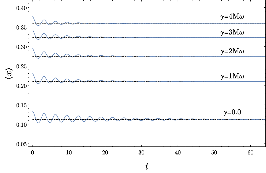
In addition we show that the steady states are stable points (i.e. attractors or sinks). To see this, we solve the master equation (7) with an initial state near to the steady states. Specifically, we chose the steady state and displaced it by a small amount. We found that with this choice of initial state the oscillator damps to the related steady state. Figure 9 shows unconditional solutions to the master equation (7) with different initial conditions (blue), each near to a steady state (dashed black line). All the solutions damp to their related steady states.

Refer to caption
Figure 9: a) Numerical (blue circles) and analytical (green line) of expectation value of phonon numbers at steady state vs γ\gamma. b) Numerical calculation of expectation value of position at steady state for differnet γ\gamma.
Refer to caption
Figure 10: Unconditional solutions to the master equation near steady state for different values of γ\gamma. Each solution eventually damps to the steady state.

Appendix D Derivation of the Master Equation

We showed the effect of Johnson noise after average over the noise and found that adding Johnson noise to the Hamiltonian will add the term due to Johnson noise (the last term of equation (31) ) to the master equation. In this section we consider an electron shuttle without Johnson noise and find its master equation in the Born-Markov approximation and at the end add the Johnson noise term to the master equation.

The Hamiltonian of the shuttle, the leads and the bosonic reservoir (for damping) is

H1\displaystyle H_{1} =H0+HI\displaystyle=H_{0}+H_{I} (45)
H0\displaystyle H_{0} =ℏ​ω​a^†​a^+ℏ​ωI​c^†​c^+∑ℓ,kωk​b^ℓ,k†​b^ℓ,k+∑pℏ​ωp​d^p†​d^p\displaystyle=\hbar\omega\hat{a}^{\dagger}\hat{a}+\hbar\omega_{I}\hat{c}^{\dagger}\hat{c}+\sum_{\ell,k}\omega_{k}\hat{b}_{\ell,k}^{\dagger}\hat{b}_{\ell,k}+\sum_{p}\hbar\omega_{p}\hat{d}_{p}^{\dagger}\hat{d}_{p} (46)
HI\displaystyle H_{I} =∑ℓ,kτℓ,k​Fℓ​(x^)​b^ℓ,k​c^†+∑pgp​a^†​d^p+h.c.\displaystyle=\sum_{\ell,k}\tau_{\ell,k}F_{\ell}(\hat{\mathrm{x}})\hat{b}_{\ell,k}\hat{c}^{\dagger}+\sum_{p}g_{p}\hat{a}^{\dagger}\hat{d}_{p}+\mathrm{h.c.} (47)

We first move to the interaction frame

HI​(t)\displaystyle H_{I}(t) =ei​H0​t/ℏHIe−iH0t/ℏ\displaystyle=e^{iH_{0}t/\hbar}H_{I}e^{-iH_{0}t/\hbar} (48)
=∑ℓ,kτℓ​k(ei​ω​a^†​a^​tFℓ(x^)e−i​ω​a^†​a^​t)(ei​ωI​c^†​c^​tc^†e−i​ωI​c^†​c^​t)(ei​∑ℓ,kωk​b^ℓ​k†​b^ℓ​k​tb^ℓ​ke−i∑ℓ,kωkb^ℓ​k†b^ℓ​kt)\displaystyle=\sum_{\ell,k}\tau_{\ell k}\left(e^{i\omega\hat{a}^{\dagger}\hat{a}t}F_{\ell}(\hat{\mathrm{x}})e^{-i\omega\hat{a}^{\dagger}\hat{a}t}\right)\left(e^{i\omega_{I}\hat{c}^{\dagger}\hat{c}t}\hat{c}^{\dagger}e^{-i\omega_{I}\hat{c}^{\dagger}\hat{c}t}\right)\left(e^{i\sum_{\ell,k}\omega_{k}\hat{b}_{\ell k}^{\dagger}\hat{b}_{\ell k}t}\hat{b}_{\ell k}e^{-i\sum_{\ell,k}\omega_{k}\hat{b}_{\ell k}^{\dagger}\hat{b}_{\ell k}t}\right)
+∑p(ei​ω​a^†​a^​ta^†e−i​ω​a^†​a^​t)(gpei​∑pωp​d^p†​d^p​td^pe−i∑pωpd^p†d^pt)+h.c.\displaystyle+\sum_{p}\left(e^{i\omega\hat{a}^{\dagger}\hat{a}t}\hat{a}^{\dagger}e^{-i\omega\hat{a}^{\dagger}\hat{a}t}\right)\left(g_{p}e^{i\sum_{p}\omega_{p}\hat{d}_{p}^{\dagger}\hat{d}_{p}t}\hat{d}_{p}e^{-i\sum_{p}\omega_{p}\hat{d}_{p}^{\dagger}\hat{d}_{p}t}\right)+\mathrm{h.c.} (49)
=∑ℓ,kτℓ​k​F~ℓ​(x^)​c^†​ei​ωI​t​b^ℓ​k​e−i​ωk​t+a^†​ei​ω​t​∑pgp​d^p​e−i​ωp​t+h.c.\displaystyle=\sum_{\ell,k}\tau_{\ell k}\tilde{F}_{\ell}(\hat{\mathrm{x}})\penalty\ \hat{c}^{\dagger}e^{i\omega_{I}t}\penalty\ \hat{b}_{\ell k}e^{-i\omega_{k}t}+\hat{a}^{\dagger}e^{i\omega t}\sum_{p}g_{p}\hat{d}_{p}e^{-i\omega_{p}t}+\mathrm{h.c.} (50)

where the time dependence of HI​(t)H_{I}(t) shows we are in the interaction frame and F~ℓ​(x^)=ei​ω​a^†​a^​t​Fℓ​(x^)​e−i​ω​a^†​a^​t\tilde{F}_{\ell}(\hat{\mathrm{x}})=e^{i\omega\hat{a}^{\dagger}\hat{a}t}F_{\ell}(\hat{\mathrm{x}})e^{-i\omega\hat{a}^{\dagger}\hat{a}t}. Then we decompose the system and bath operator by defining

C1​ℓ​(t)\displaystyle C_{1\ell}(t) ≡F~ℓ​(x^)​c^†​ei​ωI​t\displaystyle\equiv\tilde{F}_{\ell}(\hat{\mathrm{x}})\hat{c}^{\dagger}e^{i\omega_{I}t} C2​ℓ​(t)\displaystyle C_{2\ell}(t) ≡F~ℓ​(x^)​c^​e−i​ωI​t\displaystyle\equiv\tilde{F}_{\ell}(\hat{\mathrm{x}})\hat{c}e^{-i\omega_{I}t} (51a)
B1​ℓ​(t)\displaystyle B_{1\ell}(t) ≡∑kτℓ​k​b^ℓ​k​e−i​ωk​t\displaystyle\equiv\sum_{k}\tau_{\ell k}\hat{b}_{\ell k}e^{-i\omega_{k}t} B2​ℓ​(t)\displaystyle B_{2\ell}(t) ≡∑kτℓ​k​b^ℓ​k†​ei​ωk​t\displaystyle\equiv\sum_{k}\tau_{\ell k}\hat{b}_{\ell k}^{\dagger}e^{i\omega_{k}t} (51b)
A1​(t)\displaystyle A_{1}(t) ≡a^†​ei​ω​t\displaystyle\equiv\hat{a}^{\dagger}e^{i\omega t} A2​(t)\displaystyle A_{2}(t) ≡a^​e−i​ω​t\displaystyle\equiv\hat{a}e^{-i\omega t} (52a)
D1​(t)\displaystyle D_{1}(t) ≡∑pgp​d^p​e−i​ωp​t\displaystyle\equiv\sum_{p}g_{p}\hat{d}_{p}e^{-i\omega_{p}t} D2​(t)\displaystyle D_{2}(t) ≡∑pgp​d^p†​ei​ωp​t\displaystyle\equiv\sum_{p}g_{p}\hat{d}^{\dagger}_{p}e^{i\omega_{p}t} (52b)

and we write the interaction Hamiltonian in terms of these operators

HI​(t)=∑i,ℓCi​ℓ​(t)⊗Bi​ℓ​(t)+Ai​(t)⊗Di​(t).H_{I}(t)=\sum_{i,\ell}C_{i\ell}(t)\otimes B_{i\ell}(t)+A_{i}(t)\otimes D_{i}(t). (53)

Now the master equation becomes

ρ˙​(t)=\displaystyle\dot{\rho}(t)= −∑ℓ=s,d∑i,j∫0∞dτ([Ci​ℓ(t),Cj​ℓ(t−τ)ρ(t)]ℬi​jℓ(τ)+[ρ(t)Cj​ℓ(t−τ),Ci​ℓ(t)]ℬj​iℓ(−τ))\displaystyle-\sum_{\ell=s,d}\sum_{i,j}\int_{0}^{\infty}d\tau\left(\left[C_{i\ell}(t),C_{j\ell}(t-\tau)\rho(t)\right]\mathcal{B}_{ij}^{\ell}(\tau)+\left[\rho(t)C_{j\ell}(t-\tau),C_{i\ell}(t)\right]\mathcal{B}_{ji}^{\ell}(-\tau)\right)
−∑i,j∫0∞dτ([Ai(t),Aj(t−τ)ρ(t)]𝒟i​j(τ)+[ρ(t)Aj(t−τ),Ai(t)]𝒟j​i(−τ))\displaystyle-\sum_{i,j}\int_{0}^{\infty}d\tau\left(\left[A_{i}(t),A_{j}(t-\tau)\rho(t)\right]\mathcal{D}_{ij}(\tau)+\left[\rho(t)A_{j}(t-\tau),A_{i}(t)\right]\mathcal{D}_{ji}(-\tau)\right) (54)

where ℬi​jℓ​(t−t′)=⟨Bi​ℓ​(t)​Bj​ℓ​(t′)⟩E\mathcal{B}_{ij}^{\ell}(t-t^{\prime})=\langle B_{i\ell}(t)B_{j\ell}(t^{\prime})\rangle_{E} and 𝒟i​j​(t−t′)=⟨Di​(t)​Dj​(t′)⟩E\mathcal{D}_{ij}(t-t^{\prime})=\langle D_{i}(t)D_{j}(t^{\prime})\rangle_{E} are baths correlations and to calculate them we use the following averages,

⟨bℓ​k​bl​k′⟩E\displaystyle\langle b_{\ell k}b_{lk^{\prime}}\rangle_{E} =Tr​[bℓ​k​bl​k′​ρE]=0\displaystyle=\text{Tr}[b_{\ell k}b_{lk^{\prime}}\rho_{E}]=0 ⟨dp​dp′⟩E\displaystyle\langle d_{p}d_{p^{\prime}}\rangle_{E} =Tr​[dp​dp′​ρE]=0\displaystyle=\text{Tr}[d_{p}d_{p^{\prime}}\rho_{E}]=0 (55a)
⟨bℓ​k†​bl​k′†⟩E\displaystyle\langle b_{\ell k}^{\dagger}b_{lk^{\prime}}^{\dagger}\rangle_{E} =Tr​[bℓ​k†​bl​k′†​ρE]=0\displaystyle=\text{Tr}[b_{\ell k}^{\dagger}b_{lk^{\prime}}^{\dagger}\rho_{E}]=0 ⟨dp†​dp′†⟩E\displaystyle\langle d_{p}^{\dagger}d_{p^{\prime}}^{\dagger}\rangle_{E} =Tr​[dp†​dp′†​ρE]=0\displaystyle=\text{Tr}[d_{p}^{\dagger}d_{p^{\prime}}^{\dagger}\rho_{E}]=0 (55b)
⟨bℓ​k†​bl​k′⟩E\displaystyle\langle b_{\ell k}^{\dagger}b_{lk^{\prime}}\rangle_{E} =Tr​[bℓ​k†​bl​k′​ρE]=δk​k′​fℓ​(ωk)\displaystyle=\text{Tr}[b_{\ell k}^{\dagger}b_{lk^{\prime}}\rho_{E}]=\delta_{kk^{\prime}}f_{\ell}(\omega_{k}) ⟨dp†​dp′⟩E\displaystyle\langle d_{p}^{\dagger}d_{p^{\prime}}\rangle_{E} =Tr​[dp†​dp′​ρE]=δp​p′​n​(ωp)\displaystyle=\text{Tr}[d_{p}^{\dagger}d_{p^{\prime}}\rho_{E}]=\delta_{pp^{\prime}}n(\omega_{p}) (55c)
⟨bℓ​k​bl​k′†⟩E\displaystyle\langle b_{\ell k}b_{lk^{\prime}}^{\dagger}\rangle_{E} =Tr​[bℓ​k​bl​k′†​ρE]=δk​k′​(1−fℓ​(ωk))\displaystyle=\text{Tr}[b_{\ell k}b_{lk^{\prime}}^{\dagger}\rho_{E}]=\delta_{kk^{\prime}}(1-f_{\ell}(\omega_{k})) ⟨dp​dp′†⟩E\displaystyle\langle d_{p}d_{p^{\prime}}^{\dagger}\rangle_{E} =Tr​[dp​dp′†​ρE]=δp​p′​(1+n⁡(ωp))\displaystyle=\text{Tr}[d_{p}d_{p^{\prime}}^{\dagger}\rho_{E}]=\delta_{pp^{\prime}}(1+n(\omega_{p})) (55d)

where fℓ​(ωI)=1/(e(ωI−μ)/Tℓ+1)f_{\ell}(\omega_{I})=1/(e^{(\omega_{I}-\mu)/T_{\ell}}+1) is Fermi distribution of lead ℓ\ell and n⁡(ωp)=1/(eωp/T−1)n(\omega_{p})=1/(e^{\omega_{p}/T}-1) is the Bose-Einestien distribution for the cold reservoir. Using these we find

ℬ11ℓ​(t−t′)=⟨B1​ℓ​(t)​B1​ℓ​(t′)⟩E\displaystyle\mathcal{B}_{11}^{\ell}(t-t^{\prime})=\langle B_{1\ell}(t)B_{1\ell}(t^{\prime})\rangle_{E} =⟨B1​ℓ​(t−t′)​B1​ℓ​(0)⟩E=0\displaystyle=\langle B_{1\ell}(t-t^{\prime})B_{1\ell}(0)\rangle_{E}=0 (56a)
ℬ22ℓ​(t−t′)=⟨B2​ℓ​(t)​B2​ℓ​(t′)⟩E\displaystyle\mathcal{B}_{22}^{\ell}(t-t^{\prime})=\langle B_{2\ell}(t)B_{2\ell}(t^{\prime})\rangle_{E} =⟨B2​ℓ​(t−t′)​B2​ℓ​(0)⟩E=0\displaystyle=\langle B_{2\ell}(t-t^{\prime})B_{2\ell}(0)\rangle_{E}=0 (56b)
ℬ12ℓ​(t−t′)=⟨B1​ℓ​(t)​B2​ℓ​(t′)⟩E\displaystyle\mathcal{B}_{12}^{\ell}(t-t^{\prime})=\langle B_{1\ell}(t)B_{2\ell}(t^{\prime})\rangle_{E} =⟨B1​ℓ​(t−t′)​B2​ℓ​(0)⟩E\displaystyle=\langle B_{1\ell}(t-t^{\prime})B_{2\ell}(0)\rangle_{E}
=∑k​k′τℓ​k​τl​k′​⟨b^ℓ​k​b^l​k′†⟩E​e−i​ωk​(t−t′)\displaystyle=\sum_{kk^{\prime}}\tau_{\ell k}\tau_{lk^{\prime}}\langle\hat{b}_{\ell k}\hat{b}_{lk^{\prime}}^{\dagger}\rangle_{E}e^{-i\omega_{k}(t-t^{\prime})}
=∑kτℓ​k2​(1−fℓ​(ωk))​e−i​ωk​(t−t′)\displaystyle=\sum_{k}\tau_{\ell k}^{2}(1-f_{\ell}(\omega_{k}))e^{-i\omega_{k}(t-t^{\prime})}
=∫0∞d​ϵ​Jℓ​(ϵ)​(1−fℓ​(ϵ))​e−i​ϵ​(t−t′)\displaystyle=\int_{0}^{\infty}d\epsilon J_{\ell}(\epsilon)(1-f_{\ell}(\epsilon))e^{-i\epsilon(t-t^{\prime})} (56c)
ℬ21ℓ​(t−t′)=⟨B2​l​(t)​B1​ℓ​(t′)⟩E\displaystyle\mathcal{B}_{21}^{\ell}(t-t^{\prime})=\langle B_{2l}(t)B_{1\ell}(t^{\prime})\rangle_{E} =⟨B2​ℓ​(t−t′)​B1​ℓ​(0)⟩E\displaystyle=\langle B_{2\ell}(t-t^{\prime})B_{1\ell}(0)\rangle_{E}
=∑k​k′τℓ​k​τl​k′​⟨b^ℓ​k†​b^l​k′⟩E​ei​ωk​(t−t′)\displaystyle=\sum_{kk^{\prime}}\tau_{\ell k}\tau_{lk^{\prime}}\langle\hat{b}_{\ell k}^{\dagger}\hat{b}_{lk^{\prime}}\rangle_{E}e^{i\omega_{k}(t-t^{\prime})}
=∑kτℓ​k2​fℓ​(ωk)​ei​ωk​(t−t′)\displaystyle=\sum_{k}\tau_{\ell k}^{2}f_{\ell}(\omega_{k})e^{i\omega_{k}(t-t^{\prime})}
=∫0∞d​ϵ​Jℓ​(ϵ)​fℓ​(ϵ)​ei​ϵ​(t−t′)\displaystyle=\int_{0}^{\infty}d\epsilon J_{\ell}(\epsilon)f_{\ell}(\epsilon)e^{i\epsilon(t-t^{\prime})} (56d)

where we have defined the spectral density Jℓ​(ϵ)≡∑k|τℓ​k|2​δ​(ϵ−ωk)J_{\ell}(\epsilon)\equiv\sum_{k}|\tau_{\ell k}|^{2}\delta(\epsilon-\omega_{k}). Similarly we find the bosonic bath correlation

𝒟11​(t−t′)=⟨D1​(t)​D1​(t′)⟩E\displaystyle\mathcal{D}_{11}(t-t^{\prime})=\langle D_{1}(t)D_{1}(t^{\prime})\rangle_{E} =⟨D1​(t−t′)​D1⟩E=0\displaystyle=\langle D_{1}(t-t^{\prime})D_{1}\rangle_{E}=0 (57a)
𝒟22​(t−t′)=⟨D2​(t)​D2​(t′)⟩E\displaystyle\mathcal{D}_{22}(t-t^{\prime})=\langle D_{2}(t)D_{2}(t^{\prime})\rangle_{E} =⟨D2​(t−t′)​D2⟩E=0\displaystyle=\langle D_{2}(t-t^{\prime})D_{2}\rangle_{E}=0 (57b)
𝒟12​(t−t′)=⟨D1​(t)​D2​(t′)⟩E\displaystyle\mathcal{D}_{12}(t-t^{\prime})=\langle D_{1}(t)D_{2}(t^{\prime})\rangle_{E} =⟨D1​(t−t′)​D2⟩E\displaystyle=\langle D_{1}(t-t^{\prime})D_{2}\rangle_{E}
=∑p​p′gp​gp′​⟨d^d​d^p′†⟩E​e−i​ωp​(t−t′)\displaystyle=\sum_{pp^{\prime}}g_{p}g_{p^{\prime}}\langle\hat{d}_{d}\hat{d}_{p^{\prime}}^{\dagger}\rangle_{E}e^{-i\omega_{p}(t-t^{\prime})}
=∑pgp2​(1+n⁡(ωp))​e−i​ωp​(t−t′)\displaystyle=\sum_{p}g_{p}^{2}(1+n(\omega_{p}))e^{-i\omega_{p}(t-t^{\prime})}
=∫0∞d​ϵ​Jb​(ϵ)​(1+n⁡(ϵ))​e−i​ϵ​(t−t′)\displaystyle=\int_{0}^{\infty}d\epsilon J_{b}(\epsilon)(1+n(\epsilon))e^{-i\epsilon(t-t^{\prime})} (57c)
𝒟21​(t−t′)=⟨D2​(t)​D1​(t′)⟩E\displaystyle\mathcal{D}_{21}(t-t^{\prime})=\langle D_{2}(t)D_{1}(t^{\prime})\rangle_{E} =⟨D2​(t−t′)​D1⟩E\displaystyle=\langle D_{2}(t-t^{\prime})D_{1}\rangle_{E}
=∑p​p′gp​gp′​⟨b^p†​b^p′⟩E​ei​ωp​(t−t′)\displaystyle=\sum_{pp^{\prime}}g_{p}g_{p^{\prime}}\langle\hat{b}_{p}^{\dagger}\hat{b}_{p^{\prime}}\rangle_{E}e^{i\omega_{p}(t-t^{\prime})}
=∑pgp2​n​(ωp)​ei​ωp​(t−t′)\displaystyle=\sum_{p}g_{p}^{2}n(\omega_{p})e^{i\omega_{p}(t-t^{\prime})}
=∫0∞d​ω​Jb​(ϵ)​n​(ϵ)​ei​ϵ​(t−t′)\displaystyle=\int_{0}^{\infty}d\omega J_{b}(\epsilon)n(\epsilon)e^{i\epsilon(t-t^{\prime})} (57d)

where we defined spectral density of bosonic bath as Jb​(ϵ)≡∑k|gp|2​δ​(ϵ−ωp)J_{b}(\epsilon)\equiv\sum_{k}|g_{p}|^{2}\delta(\epsilon-\omega_{p}). Using these correlation functions, we write the master equation as sum of integrals,

ρ˙(t)=−∑ℓ=s,d∑i=14ℐiℓ−∑i=14𝒦i\dot{\rho}(t)=-\sum_{\ell=s,d}\sum_{i=1}^{4}\mathcal{I}_{i}^{\ell}-\sum_{i=1}^{4}\mathcal{K}_{i} (58)

where ℐiℓ\mathcal{I}_{i}^{\ell}s are integrals for lead ℓ\ell as follows

ℐ1ℓ\displaystyle\mathcal{I}_{1}^{\ell} =∫0∞d​τ​[C1​ℓ​(t),C2​ℓ​(t−τ)​ρ​(t)]​ℬ12ℓ​(τ)\displaystyle=\int_{0}^{\infty}d\tau\left[C_{1\ell}(t),C_{2\ell}(t-\tau)\rho(t)\right]\mathcal{B}_{12}^{\ell}(\tau)
=∫0∞d​τ​[F~ℓ​c^†​ei​ωI​t,F~ℓ​c^​e−i​ωI​(t−τ)​ρ​(t)]​∫0∞d​ϵ​Jℓ​(ϵ)​(1−fℓ​(ϵ))​e−i​ϵ​τ\displaystyle=\int_{0}^{\infty}d\tau\left[\tilde{F}_{\ell}\hat{c}^{\dagger}e^{i\omega_{I}t},\tilde{F}_{\ell}\hat{c}e^{-i\omega_{I}(t-\tau)}\rho(t)\right]\int_{0}^{\infty}d\epsilon J_{\ell}(\epsilon)(1-f_{\ell}(\epsilon))e^{-i\epsilon\tau}
=[F~ℓ​c^†,F~ℓ​c^​ρ​(t)]​∫0∞d​τ​∫0∞d​ϵ​J​(ϵ)​(1−fℓ​(ϵ))​ei⁡(ωI−ϵ)​τ\displaystyle=[\tilde{F}_{\ell}\hat{c}^{\dagger},\tilde{F}_{\ell}\hat{c}\rho(t)]\int_{0}^{\infty}d\tau\int_{0}^{\infty}d\epsilon J(\epsilon)(1-f_{\ell}(\epsilon))e^{i(\omega_{I}-\epsilon)\tau} (59)
=[F~ℓ​c^†,F~ℓ​c^​ρ​(t)]​Γℓ​(ωI)2​(1−fℓ​(ωI))\displaystyle=[\tilde{F}_{\ell}\hat{c}^{\dagger},\tilde{F}_{\ell}\hat{c}\rho(t)]\frac{\Gamma_{\ell}(\omega_{I})}{2}(1-f_{\ell}(\omega_{I})) (60)
ℐ2ℓ\displaystyle\mathcal{I}_{2}^{\ell} =∫0∞d​τ​[ρ⁡(t)​C2​ℓ​(t−τ),C1​ℓ​(t)]​ℬ21ℓ​(−τ)\displaystyle=\int_{0}^{\infty}d\tau\left[\rho(t)C_{2\ell}(t-\tau),C_{1\ell}(t)\right]\mathcal{B}_{21}^{\ell}(-\tau)
=∫0∞d​τ​[ρ⁡(t)​F~ℓ​c^​e−i​ωI​(t−τ),F~ℓ​c^†​ei​ωI​t]​∫0∞d​ϵ​Jℓ​(ϵ)​fℓ​(ϵ)​e−i​ϵ​τ\displaystyle=\int_{0}^{\infty}d\tau\left[\rho(t)\tilde{F}_{\ell}\hat{c}e^{-i\omega_{I}(t-\tau)},\tilde{F}_{\ell}\hat{c}^{\dagger}e^{i\omega_{I}t}\right]\int_{0}^{\infty}d\epsilon J_{\ell}(\epsilon)f_{\ell}(\epsilon)e^{-i\epsilon\tau}
=[ρ⁡(t)​F~ℓ​c^,F~ℓ​c^†]​∫0∞d​τ​∫0∞d​ϵ​Jℓ​(ϵ)​fℓ​(ϵ)​ei⁡(ωI−ϵ)​τ\displaystyle=[\rho(t)\tilde{F}_{\ell}\hat{c},\tilde{F}_{\ell}\hat{c}^{\dagger}]\int_{0}^{\infty}d\tau\int_{0}^{\infty}d\epsilon J_{\ell}(\epsilon)f_{\ell}(\epsilon)e^{i(\omega_{I}-\epsilon)\tau} (61)
=[ρ⁡(t)​F~ℓ​c^,F~ℓ​c^†]​Γℓ​(ωI)2​fℓ​(ωI)\displaystyle=[\rho(t)\tilde{F}_{\ell}\hat{c},\tilde{F}_{\ell}\hat{c}^{\dagger}]\frac{\Gamma_{\ell}(\omega_{I})}{2}f_{\ell}(\omega_{I}) (62)
ℐ3ℓ\displaystyle\mathcal{I}_{3}^{\ell} =∫0∞d​τ​[C2​ℓ​(t),C1​ℓ​(t−τ)​ρ​(t)]​ℬ21ℓ​(τ)\displaystyle=\int_{0}^{\infty}d\tau\left[C_{2\ell}(t),C_{1\ell}(t-\tau)\rho(t)\right]\mathcal{B}_{21}^{\ell}(\tau)
=∫0∞d​τ​[F~ℓ​c^​e−i​ωI​t,F~ℓ​c^†​ei​ωI​(t−τ)​ρ​(t)]​∫0∞d​ϵ​Jℓ​(ϵ)​fℓ​(ϵ)​ei​ϵ​τ\displaystyle=\int_{0}^{\infty}d\tau\left[\tilde{F}_{\ell}\hat{c}e^{-i\omega_{I}t},\tilde{F}_{\ell}\hat{c}^{\dagger}e^{i\omega_{I}(t-\tau)}\rho(t)\right]\int_{0}^{\infty}d\epsilon J_{\ell}(\epsilon)f_{\ell}(\epsilon)e^{i\epsilon\tau}
=[F~ℓ​c^,F~ℓ​c^†​ρ​(t)]​∫0∞d​τ​∫0∞d​ϵ​Jℓ​(ϵ)​fℓ​(ϵ)​e−i⁡(ωI−ϵ)​τ\displaystyle=[\tilde{F}_{\ell}\hat{c},\tilde{F}_{\ell}\hat{c}^{\dagger}\rho(t)]\int_{0}^{\infty}d\tau\int_{0}^{\infty}d\epsilon J_{\ell}(\epsilon)f_{\ell}(\epsilon)e^{-i(\omega_{I}-\epsilon)\tau} (63)
=[F~ℓ​c^,F~ℓ​c^†​ρ​(t)]​Γℓ​(ωI)2​fℓ​(ωI)\displaystyle=[\tilde{F}_{\ell}\hat{c},\tilde{F}_{\ell}\hat{c}^{\dagger}\rho(t)]\frac{\Gamma_{\ell}(\omega_{I})}{2}f_{\ell}(\omega_{I}) (64)
ℐ4ℓ\displaystyle\mathcal{I}_{4}^{\ell} =∫0∞d​τ​[ρ⁡(t)​C1​ℓ​(t−τ),C2​ℓ​(t)]​ℬ12ℓ​(−τ)\displaystyle=\int_{0}^{\infty}d\tau\left[\rho(t)C_{1\ell}(t-\tau),C_{2\ell}(t)\right]\mathcal{B}_{12}^{\ell}(-\tau)
=∫0∞d​τ​[ρ⁡(t)​F~ℓ​c^†​ei​ωI​(t−τ),F~ℓ​c^​e−i​ωI​t]​∫0∞d​ϵ​Jℓ​(ϵ)​(1−fℓ​(ϵ))​ei​ϵ​τ\displaystyle=\int_{0}^{\infty}d\tau\left[\rho(t)\tilde{F}_{\ell}\hat{c}^{\dagger}e^{i\omega_{I}(t-\tau)},\tilde{F}_{\ell}\hat{c}e^{-i\omega_{I}t}\right]\int_{0}^{\infty}d\epsilon J_{\ell}(\epsilon)(1-f_{\ell}(\epsilon))e^{i\epsilon\tau}
=[ρ⁡(t)​F~ℓ​c^†,F~ℓ​c^]​∫0∞d​τ​∫0∞d​ϵ​Jℓ​(ϵ)​(1−fℓ​(ϵ))​e−i⁡(ωI−ϵ)​τ\displaystyle=[\rho(t)\tilde{F}_{\ell}\hat{c}^{\dagger},\tilde{F}_{\ell}\hat{c}]\int_{0}^{\infty}d\tau\int_{0}^{\infty}d\epsilon J_{\ell}(\epsilon)(1-f_{\ell}(\epsilon))e^{-i(\omega_{I}-\epsilon)\tau} (65)
=[ρ⁡(t)​F~ℓ​c^†,F~ℓ​c^]​Γℓ​(ωI)2​(1−fℓ​(ωI))\displaystyle=[\rho(t)\tilde{F}_{\ell}\hat{c}^{\dagger},\tilde{F}_{\ell}\hat{c}]\frac{\Gamma_{\ell}(\omega_{I})}{2}(1-f_{\ell}(\omega_{I})) (66)

and 𝒦i\mathcal{K}_{i} are integrals for bosonic bath,

𝒦1\displaystyle\mathcal{K}_{1} =∫0∞d​τ​[A1​(t),A2​(t−τ)​ρ​(t)]​𝒟12​(τ)\displaystyle=\int_{0}^{\infty}d\tau\left[A_{1}(t),A_{2}(t-\tau)\rho(t)\right]\mathcal{D}_{12}(\tau)
=∫0∞d​τ​[a^†​ei​ω​t,a^​e−i​ω​(t−τ)​ρ​(t)]​∫0∞d​ϵ​Jb​(ϵ)​(1+n⁡(ϵ))​e−i​ϵ​τ\displaystyle=\int_{0}^{\infty}d\tau\left[\hat{a}^{\dagger}e^{i\omega t},\hat{a}e^{-i\omega(t-\tau)}\rho(t)\right]\int_{0}^{\infty}d\epsilon J_{b}(\epsilon)(1+n(\epsilon))e^{-i\epsilon\tau}
=[a^†,a^​ρ​(t)]​∫0∞d​τ​∫0∞d​ϵ​Jb​(ϵ)​(1+n⁡(ϵ))​ei⁡(ω−ϵ)​τ\displaystyle=[\hat{a}^{\dagger},\hat{a}\rho(t)]\int_{0}^{\infty}d\tau\int_{0}^{\infty}d\epsilon J_{b}(\epsilon)(1+n(\epsilon))e^{i(\omega-\epsilon)\tau} (67)
=[a^†,a^​ρ​(t)]​κ⁡(ω)2​(1+n⁡(ω))\displaystyle=[\hat{a}^{\dagger},\hat{a}\rho(t)]\frac{\kappa(\omega)}{2}(1+n(\omega)) (68)
𝒦2\displaystyle\mathcal{K}_{2} =∫0∞d​τ​[ρ⁡(t)​A2​(t−τ),A1​(t)]​𝒟21​(−τ)\displaystyle=\int_{0}^{\infty}d\tau\left[\rho(t)A_{2}(t-\tau),A_{1}(t)\right]\mathcal{D}_{21}(-\tau)
=∫0∞d​τ​[ρ⁡(t)​a^​e−i​ω​(t−τ),a^†​ei​ω​t]​∫0∞d​ϵ​Jb​(ϵ)​n​(ϵ)​e−i​ϵ​τ\displaystyle=\int_{0}^{\infty}d\tau\left[\rho(t)\hat{a}e^{-i\omega(t-\tau)},\hat{a}^{\dagger}e^{i\omega t}\right]\int_{0}^{\infty}d\epsilon J_{b}(\epsilon)n(\epsilon)e^{-i\epsilon\tau}
=[ρ⁡(t)​a^,a^†]​∫0∞d​τ​∫0∞d​ϵ​Jb​(ϵ)​n​(ϵ)​ei⁡(ω−ϵ)​τ\displaystyle=[\rho(t)\hat{a},\hat{a}^{\dagger}]\int_{0}^{\infty}d\tau\int_{0}^{\infty}d\epsilon J_{b}(\epsilon)n(\epsilon)e^{i(\omega-\epsilon)\tau} (69)
=[ρ⁡(t)​a^,a^†]​κ⁡(ω)2​n​(ω)\displaystyle=[\rho(t)\hat{a},\hat{a}^{\dagger}]\frac{\kappa(\omega)}{2}n(\omega) (70)
𝒦3\displaystyle\mathcal{K}_{3} =∫0∞d​τ​[A2​(t),A1​(t−τ)​ρ​(t)]​𝒟21​(τ)\displaystyle=\int_{0}^{\infty}d\tau\left[A_{2}(t),A_{1}(t-\tau)\rho(t)\right]\mathcal{D}_{21}(\tau)
=∫0∞d​τ​[a^​e−i​ω​t,a^†​ei​ω​(t−τ)​ρ​(t)]​∫0∞d​ϵ​Jb​(ϵ)​n​(ϵ)​ei​ϵ​τ\displaystyle=\int_{0}^{\infty}d\tau\left[\hat{a}e^{-i\omega t},\hat{a}^{\dagger}e^{i\omega(t-\tau)}\rho(t)\right]\int_{0}^{\infty}d\epsilon J_{b}(\epsilon)n(\epsilon)e^{i\epsilon\tau}
=[a^,a^†​ρ​(t)]​∫0∞d​τ​∫0∞d​ϵ​Jb​(ϵ)​n​(ϵ)​e−i⁡(ω−ϵ)​τ\displaystyle=[\hat{a},\hat{a}^{\dagger}\rho(t)]\int_{0}^{\infty}d\tau\int_{0}^{\infty}d\epsilon J_{b}(\epsilon)n(\epsilon)e^{-i(\omega-\epsilon)\tau} (71)
=[a^,a^†​ρ​(t)]​κ⁡(ω)2​n​(ω)\displaystyle=[\hat{a},\hat{a}^{\dagger}\rho(t)]\frac{\kappa(\omega)}{2}n(\omega) (72)
𝒦4\displaystyle\mathcal{K}_{4} =∫0∞d​τ​[ρ⁡(t)​A1​(t−τ),A2​(t)]​𝒟12​(−τ)\displaystyle=\int_{0}^{\infty}d\tau\left[\rho(t)A_{1}(t-\tau),A_{2}(t)\right]\mathcal{D}_{12}(-\tau)
=∫0∞d​τ​[ρ⁡(t)​a^†​ei​ω​(t−τ),a^​e−i​ω​t]​∫0∞d​ϵ​Jb​(ϵ)​(1+n⁡(ϵ))​ei​ϵ​τ\displaystyle=\int_{0}^{\infty}d\tau\left[\rho(t)\hat{a}^{\dagger}e^{i\omega(t-\tau)},\hat{a}e^{-i\omega t}\right]\int_{0}^{\infty}d\epsilon J_{b}(\epsilon)(1+n(\epsilon))e^{i\epsilon\tau}
=[ρ⁡(t)​a^†,a^]​∫0∞d​τ​∫0∞d​ϵ​Jb​(ϵ)​(1+n⁡(ϵ))​e−i⁡(ω−ϵ)​τ\displaystyle=[\rho(t)\hat{a}^{\dagger},\hat{a}]\int_{0}^{\infty}d\tau\int_{0}^{\infty}d\epsilon J_{b}(\epsilon)(1+n(\epsilon))e^{-i(\omega-\epsilon)\tau} (73)
=[ρ⁡(t)​a^†,a^]​κ⁡(ω)2​(1+n⁡(ω))\displaystyle=[\rho(t)\hat{a}^{\dagger},\hat{a}]\frac{\kappa(\omega)}{2}(1+n(\omega)) (74)

We used the following relation to calculate the time integrals

∫0∞d​t​e±i​ϵ​t=π​δ​(ϵ)±i​Pϵ,\int_{0}^{\infty}dte^{\pm i\epsilon t}=\pi\delta(\epsilon)\pm i\frac{P}{\epsilon}, (75)

where PP denotes the Cauchy principal value. We only use the real part of the integral since the imaginary part can be absorbed into H0H_{0}. Also we defind the following zero temperature rates

Γℓ​(ϵ)\displaystyle\Gamma_{\ell}(\epsilon) =2​π​Jℓ​(ϵ)\displaystyle=2\pi J_{\ell}(\epsilon) (76)
κ⁡(ϵ)\displaystyle\kappa(\epsilon) =2​π​Jb​(ϵ).\displaystyle=2\pi J_{b}(\epsilon). (77)

Now we write the master equation by adding the calculated integrals

ρ˙​(t)\displaystyle\dot{\rho}(t) =−∑ℓ=s,d\displaystyle=-\sum_{\ell=s,d} (Γℓ2​(1−fℓ​(ωI))​[F~ℓ​c^†,F~ℓ​c^​ρ​(t)]+Γℓ2​fℓ​(ωI)​[ρ⁡(t)​F~ℓ​c^,F~ℓ​c^†]CLOSE\displaystyle\left(\frac{\Gamma_{\ell}}{2}(1-f_{\ell}(\omega_{I}))[\tilde{F}_{\ell}\hat{c}^{\dagger},\tilde{F}_{\ell}\hat{c}\rho(t)]+\frac{\Gamma_{\ell}}{2}f_{\ell}(\omega_{I})[\rho(t)\tilde{F}_{\ell}\hat{c},\tilde{F}_{\ell}\hat{c}^{\dagger}]\right.
+\displaystyle+ OPENΓℓ2​fℓ​(ωI)​[F~ℓ​c^,F~ℓ​c^†​ρ​(t)]+Γℓ2​(1−fℓ​(ωI))​[ρ⁡(t)​F~ℓ​c^†,F~ℓ​c^])\displaystyle\left.\frac{\Gamma_{\ell}}{2}f_{\ell}(\omega_{I})[\tilde{F}_{\ell}\hat{c},\tilde{F}_{\ell}\hat{c}^{\dagger}\rho(t)]+\frac{\Gamma_{\ell}}{2}(1-f_{\ell}(\omega_{I}))[\rho(t)\tilde{F}_{\ell}\hat{c}^{\dagger},\tilde{F}_{\ell}\hat{c}]\right)
−\displaystyle- (κ2​(1+n⁡(ω))​[a^†,a^​ρ​(t)]+κ2​n​(ω)​[ρ⁡(t)​a^,a^†]CLOSE\displaystyle\left(\frac{\kappa}{2}(1+n(\omega))[\hat{a}^{\dagger},\hat{a}\rho(t)]+\frac{\kappa}{2}n(\omega)[\rho(t)\hat{a},\hat{a}^{\dagger}]\right.
+\displaystyle+ OPENκ2​n​(ω)​[a^,a^†​ρ​(t)]+κ2​(1+n⁡(ω))​[ρ⁡(t)​a^†,a^])\displaystyle\left.\frac{\kappa}{2}n(\omega)[\hat{a},\hat{a}^{\dagger}\rho(t)]+\frac{\kappa}{2}(1+n(\omega))[\rho(t)\hat{a}^{\dagger},\hat{a}]\right)
=−∑ℓ=s,d\displaystyle=-\sum_{\ell=s,d} (Γℓ2​(1−fℓ​(ωI))​([F~ℓ​c^†,F~ℓ​c^​ρ​(t)]+[ρ⁡(t)​F~ℓ​c^†,F~ℓ​c^])+Γℓ2​fℓ​(ωI)​([ρ⁡(t)​F~ℓ​c^,F~ℓ​c^†]+[F~ℓ​c^,F~ℓ​c^†​ρ​(t)]))\displaystyle\left(\frac{\Gamma_{\ell}}{2}(1-f_{\ell}(\omega_{I}))\left([\tilde{F}_{\ell}\hat{c}^{\dagger},\tilde{F}_{\ell}\hat{c}\rho(t)]+[\rho(t)\tilde{F}_{\ell}\hat{c}^{\dagger},\tilde{F}_{\ell}\hat{c}]\right)+\frac{\Gamma_{\ell}}{2}f_{\ell}(\omega_{I})\left([\rho(t)\tilde{F}_{\ell}\hat{c},\tilde{F}_{\ell}\hat{c}^{\dagger}]+[\tilde{F}_{\ell}\hat{c},\tilde{F}_{\ell}\hat{c}^{\dagger}\rho(t)]\right)\right)
−\displaystyle- (κ2​(1+n⁡(ω))​([a^†,a^​ρ​(t)]+[ρ⁡(t)​a^†,a^])+κ2​n​(ω)​([ρ⁡(t)​a^,a^†]+[a^,a^†​ρ​(t)]))\displaystyle\left(\frac{\kappa}{2}(1+n(\omega))\left([\hat{a}^{\dagger},\hat{a}\rho(t)]+[\rho(t)\hat{a}^{\dagger},\hat{a}]\right)+\frac{\kappa}{2}n(\omega)\left([\rho(t)\hat{a},\hat{a}^{\dagger}]+[\hat{a},\hat{a}^{\dagger}\rho(t)]\right)\right)
=∑ℓ=s,d\displaystyle=\sum_{\ell=s,d} (Γℓ​(1−fℓ​(ωI))​ℒ​[F~ℓ​c^]​ρ+Γℓ​fℓ​(ωI)​ℒ​[F~ℓ​c^†]​ρ)+(κ⁡(1+n⁡(ω))​ℒ​[a^]​ρ+κ​n​(ω)​ℒ​[a^†]​ρ).\displaystyle\left(\Gamma_{\ell}(1-f_{\ell}(\omega_{I}))\mathcal{L}[\tilde{F}_{\ell}\hat{c}]\rho+\Gamma_{\ell}f_{\ell}(\omega_{I})\mathcal{L}[\tilde{F}_{\ell}\hat{c}^{\dagger}]\rho\right)+\left(\kappa(1+n(\omega))\mathcal{L}[\hat{a}]\rho+\kappa n(\omega)\mathcal{L}[\hat{a}^{\dagger}]\rho\right). (78)

And the master equation in its final form is

ρ˙​(t)\displaystyle\dot{\rho}(t) =Γs​(1−fs​(ωI))​ℒ​[F~s​c^]​ρ+Γs​fs​(ωI)​ℒ​[F~s​c^†]​ρ\displaystyle=\Gamma_{s}(1-f_{s}(\omega_{I}))\mathcal{L}[\tilde{F}_{s}\hat{c}]\rho+\Gamma_{s}f_{s}(\omega_{I})\mathcal{L}[\tilde{F}_{s}\hat{c}^{\dagger}]\rho
+Γd​(1−fd​(ωI))​ℒ​[F~d​c^]​ρ+Γℓ​fd​(ωI)​ℒ​[F~d​c^†]​ρ\displaystyle+\Gamma_{d}(1-f_{d}(\omega_{I}))\mathcal{L}[\tilde{F}_{d}\hat{c}]\rho+\Gamma_{\ell}f_{d}(\omega_{I})\mathcal{L}[\tilde{F}_{d}\hat{c}^{\dagger}]\rho
+κ⁡(1+n⁡(ω))​ℒ​[a^]​ρ+κ​n​(ω)​ℒ​[a^†]​ρ\displaystyle+\kappa(1+n(\omega))\mathcal{L}[\hat{a}]\rho+\kappa n(\omega)\mathcal{L}[\hat{a}^{\dagger}]\rho (79)

Appendix E Evidence for Stochastic Resonance

In this section we show the evidence for existence of Stochastic Resonance.

The following table of histograms shows the momentum distribution of solutions to the conditional master equation. The value of γ\gamma is increasing from top to bottom and each histogram at each row is a different trajectory for the same parameters. Gaussian fit shown in blue curve and the residual is shown below each histogram.

Gaussian fit matches pretty well and show the oscillator is mostly in thermal equilibrium. In the middle of histograms, some disagreements with the gaussian fit are seen. These are due to non equilibrium state of the oscillator after electron jumps.

[Uncaptioned image]

The following 3D histograms show distribution of the phase space coordinates over 400 cycles. Similar to the previous table of histograms, the value of γ\gamma increases from top to bottom and each histogram at each row represents a different trajectory for the same parameters. The ‘crater-like’ depression in the centre of these histograms suggests the existence of a stochastic resonance.

[Uncaptioned image]

Following figures show the power spectrum of the position (Sx​(ω~)S_{x}(\tilde{\omega})) and the velocity (Sv​(ω~)S_{v}(\tilde{\omega})). The peak at ω~≈2.0​ω\tilde{\omega}\approx 2.0\omega shows stochastic resonance frequency.

[Uncaptioned image]
[Uncaptioned image]