Coupling of skyrmions mediated by RKKY interaction
Abstract
A discussion on the interaction between skyrmions in a bi-layer system connected by a non-magnetic metal is presented. From considering a free charge carrier model, we have shown that the Ruderman-Kittel-Kasuya-Yosida () interaction can induce attractive or repulsive interaction between the skyrmions depending on the spacer thickness. We have also shown that due to an increasing in RKKY energy when the skyrmions are far from each other, their widths are diminished. Finally, we have obtained analytical solutions to the skyrmion position when the in-plane distance between the skyrmions is small and it is shown that an attractive RKKY interaction yields a skyrmion precessory motion. This RKKY-induced coupling could be used as a skyrmion drag mechanism to displace skyrmions in multilayers.
The possibility of using magnetic patterns such as vortices [1], domain walls [2] and skyrmions [3] in spintronic devices has resulted in an increasing interest in studying statical and dynamical properties of these magnetization collective modes. In particular, skyrmions are topological spin textures that may appear as groundstate in non-centrosymmetric crystals in the presence of the bulk Dzyaloshinskii-Moriya interaction () [4, 5, 6, 7, 8]. Due to their topological stability, small size and low driving magnetic field/current density [9, 10], skyrmions are also promising candidates to compose spintronic devices based on the interesting concept of racetrack memory [3, 11, 12], as well as in logic devices [13, 14] and spin transfer nano-oscillators [15, 16].
Nevertheless, as a consequence of the skyrmion Hall effect, the use of these objects in racetrack devices is strongly hampered because a skyrmion cannot move in a straight line along the driving current or external magnetic field direction. Therefore, magnetic skyrmions can be destroyed at the edges of nanostripes[17, 18]. A possible way to avoid the skyrmion Hall effect is the coupling between two skyrmions lying in different layers. In fact, when two skyrmions are on separate planes, changes in the interlayer exchange interaction and the signs of the can induce different statical and dynamical properties of the magnetization [19]. In this context, it has been shown that the Skyrmion Hall effect can be suppressed by considering two perpendicularly magnetized ferromagnetic sublayers strongly coupled via an antiferromagnetic exchange interaction [20]. Furthermore, skyrmions belonging to different layers can move simultaneously. That is, the skyrmion in the layer without current follows the motion of the skyrmion belonging to the layer in which an electrical current is injected [20]. From experimental point of view, a superimposition of skyrmions can be obtained from the strong dipolar stray field of two skyrmions, which behave as a single particle [21].
In this paper, we study the statical and dynamical properties of two skyrmions in superimposed layers connected by a non-magnetic conductor material. The presence of the conductor causes the magnetic layers interact through the Ruderman-Kittel-Kasuya-Yosida() interaction[22, 23, 24, 25, 26]. The interaction is one of the most important and frequently discussed couplings between the localized magnetic moments in solids and adatoms interactions[27, 28, 29, 30]. Particularly, concerning topological objects, this interaction has been proposed as a mechanism to stabilize an isolated magnetic skyrmion in a magnetic monolayer on a nonmagnetic conducting substrate [31]. Here, we show that due to the oscillatory signal of interaction as a function of the spacer thickness, the interaction between skyrmions placed in different layers can be attractive or repulsive. Additionally, we show that the skyrmion radius diminishes when the skyrmions are far from each other, recovering their widths of isolated skyrmions when they are superimposed. Finally, we obtain an interaction potential for the case of ferromagnetic coupling and solve the Thiele’s equation aiming to describe the skyrmion dynamics when the in-plane distance between the two skyrmions is small.
The considered magnetic system consists of two rectangular monolayer with dimensions and separated by a non-magnetic metal with thickness (See Fig. 1). The layer spacer consists of a conductor material and the electrons are described as free charge carrier, whose formula to interaction is well established [26, 32]. Without lost of generality, it is assumed that the skyrmion placed in the lower layer is located at the origin of the adopted coordinate system in such way that the magnetization pattern of the layers comprises a skyrmion positioned in the coordinate and a skyrmion at , where the subindices and refer respectively to the upper and lower layer.

The magnetic energy of an arbitrary magnetization profile will be given by , where , e are respectively the energies coming from exchange, Dzyaloshinskii-Moriya and interactions. It is important to note that if the magnetic properties of the system is described only in terms of exchange and DMI interactions, helical states are predicted to appear [33]. Nevertheless, despite anisotropy and Zeeman interactions are important to ensure skyrmion stability, for our purposes, the knowledge on exchange and DMI energies is enough to describe our results. For more details and analysis of another terms to the magnetic energy, see Ref. [34].
In the continuous limit, the exchange and energies are respectively given by
| (1) |
and
where is the unitary vector describing the magnetization direction, is the saturation magnetization of the material, is the exchange constant and is the constant. The interaction will be determined from a continuous approximation considering that the properties of the non-magnetic material connecting the layers can be well described by a free electron gas. In this context, the energy coming from the interaction between two magnetic moments is given by [22, 25, 26], where is a magnetic moment in layer , is a magnetic moment in layer , is the function that determines the coupling between two magnetic moments belonging to different layers, is the Fermi vector of the conductor material and is the distance between two magnetic moments in different layers. For a free electron gas, the function is given by [32]
| (3) |
where , is the exchange interaction between electrons in the magnetic layer and conduction electrons, is the effective mass of the conduction electrons and is the Planck constant. It can be observed that, due to the periodicity of trigonometric functions, the coupling between two magnetic moments can be ferromagnetic or antiferromagnetic, depending on the distance between them. The total interaction energy is given by the sum of all pairs of magnetic moments of the bi-layer. Thus, in a continuous approximation, the energy can be written as
| (4) |
where is the surface area of a unitary cell of the magnetic material and the integrals are performed along the surfaces of the two magnetic layers. It is important to note that the interaction is inversely proportional to and for , oscillates with a period and decays as [25].
In the adopted model, the magnetization vector field is considered as a continuous function depending on the position inside the magnetic layer. There are several ansatz describing the magnetization profile of a skyrmion [35, 36, 37, 38, 39]. In this work, we use the ansatz of Refs. [40, 34], in which the magnetization is parametrized as , with
| (5) |
where is the skyrmion characteristic length and . The subindex describes the layer in which the skyrmion lies, that is, for layer and for layer . Therefore, Eq.(1) can be rewritten as
| (6) |
Subindex in the sum refers to (1) and (2) coordinates. In addition, Eq. (Coupling of skyrmions mediated by RKKY interaction) is also rewritten as
| (7) |
From the described model we are in position to calculate the total magnetic energy of the bi-layer system. Therefore, from considering that the skyrmions are far from the borders of the stripe, the exchange and energies of the described skyrmion profile are given respectively by and , where
It can be noted that, in the limit , the exchange energy of the skyrmions is and , which is in accord to the energy of solitonic solutions of the non-linear -model [42]. Figure 2 shows the skyrmion energy as a function of its width for different . It can be noted that, despite the energy decreases when increases, there is no qualitative changes of the value that minimizes the magnetic energy. This is associated with the fact that we are not considering anisotropy or Zeeman interactions in this work. For more details and analysis on the skyrmion size, see Ref. [41].


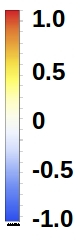
Our main goal in this work is to determine the magnetic energy when the skyrmions are separated by a conductor layer. Nevertheless, an expression for energy is hard to be obtained analytically and so, it is numerically solved by the integration of Eq.(4). We consider that the conductor material is a copper layer for which . The integration along all the region of the stripe demands a very long computational time. Therefore, aiming to obtain numerical results faster, we have performed the numerical integration by cutting the integration region. That is, we have calculated the energy of one magnetic moment located in layer with the magnetic moments located inside a square of side in the layer . This procedure was performed for all magnetic moments in layer . It is noted that differences in the obtained energy values starts to be negligible when the square side is on the order of nm. Thus, by using this value to the square side, we have calculated the energy as a function of the spacer thickness and the skyrmion position along -direction. The main results are summarized in Fig.3, in which it can be noted that due to the periodicity of the interaction, the skyrmion-skyrmion interaction can be attractive or repulsive, depending on the interlayer thickness. We have also performed the numerical integration of Eq.(4) for different values of aiming to understand how interaction influences the skyrmion width; the results are shown in Fig.4. We have obtained that the energy depends on the skyrmon width only when they are far away one to another. That is, for large distances, the skyrmion radius diminishes aiming to reduce energy. However, when the distance between them decreases, energy is independent of the skyrmion width and then, when the skyrmions are superimposed, their widths must be determined by the interplay among uniaxial anisotropy, exchange and interactions, being equal to the isolated skyrmion width [34, 41].
We will now describe the skyrmion dynamics from considering two layers in the absence of currents and external magnetic fields. Additionaly, we will assume that the in-plane skymion distance is on the order of because, for larger distances, the potential coming from interaction is practically constant. In our analytical model, we neglect the dynamical deformation of the skyrmions in such way that, the Landau-Lifshitz-Gilbert equation can be reduced to the Thiele equation[43], written as
| (8) |
where subscripts label the layers ( and ). The first term in the above equation describes the Magnus force exerted by the magnetic texture in the magnetic skyrmion located in the -th layer, which displaces with velocity . Once we are considering the dynamics of a highly symmetrical skyrmion, we have that , where is the gyromagnetic ratio. The second term represents the dissipative force action in each magnetic skyrmion. The right side of Eq.(8) represents the force that determines the skyrmions dynamics, which contains a contribution from the potential , originated from the skyrmion-skyrmion interaction. From the results obtained to the energy, we can state that when is very small, the interaction energy between skyrmions is given by a harmonic potential , where depends on the layer distance and the conductor parameters and is the distance between the skyrmions along the -plane. From Fig. 3 one can note that this approximation is very good when the skyrmion centers are separated by a distance nm. On the other hand, in the asymptotic limit , the interaction energy is almost constant and comes from the interaction of the skyrmion in layer with the ferromagnetic state in layer and vice-versa, with . In these asymptotic limits, we can obtain the analytical solution to Eq.(8) and it is presented into the Appendix A. By using the result given in Fig.3, we can also assume that the potential in the intermediary zone (that is, ) can be very well represented by (See Fig. 3a). From estimating Jm, we have obtained the position of the skyrmions for nm as a function of time and the results can be viewed in Fig. 5. It can be noted that when the in-plane distance between skyrmions is on the order of , a drag effect is observed and an attractive interaction is observed in such way that the two skyrmions become coupled, precessing one around other with frequency . This precessory motion is resulted from the interplay between skyrmion-skyrmion attraction and the Magnus force exerted by the magnetic texture in the magnetic skyrmions. In this way, when the skyrmions move one towards the other, the skyrmion Hall effect produces a displacement of skyrmions in opposite directions and the resulting motion is that one shown in Fig. 5b. The skyrmions can be decoupled by changing the interlayer distance when an antiferromagnetic interaction appears.


The observed skyrmion coupling is a very interesting result because it opens the possibility to realize devices based on the concept of skyrmion drag effects. That is, if it is possible to apply different in-plane magnetic fields or different anisotropies in layers and , the skyrmions can displace with different velocities; however, when the distance between them is small, skyrmions couple and can displace together, which can diminishes the skyrmion Hall effect due to the increasing of the effective skyrmion mass. In addition, a magnetoresistive device can be proposed because there is a decreasing in the resistence when the skyrmion are superimposed. In fact, the value of an electric current passing through the multilayer system in the direction perpendicular to the planes depends on the skyrmion positions because magnetoresistive effects take place and the resistence diminishes when the skyrmions are superimposed.
In conclusion, we have described the coupling between skyrmions in different layers separated by a conductor non-magnetic material. It has been shown that the interaction can lead to a skyrmion coupling/decoupling, depending on the spacer thickness. The skyrmion radius is also affected by interaction in such way that it diminishes when the skyrmions are far from each other and it increases when they are in an small in-plane distance. The dynamics of this system show that when skyrmions in different layers are put near one to another, they execute a precession motion around each other. The drag effect mediated by can be used to move skyrmions in different layers with the same velocity.
References
- [1] D. Kumar, S. Barman, and A. Barman, Sci. Rep. 4, 04108 (2014).
- [2] G. Catalan, J. Seidel, R. Ramesh, and J. F. Scott, Rev. Mod. Phys. 84, 119 (2012).
- [3] R. Tomasello, E. Martinez, R. Zivieri, L. Torres, M. Carpentieri, G. Finocchio, Sci. Rep. 4, 6784 (2014).
- [4] W. Jiang, G. Chen, K. Liu, J. Zang, S.G.E. te Velthuis, and A. Hoffmann, Phys. Reports 704, 1 (2017).
- [5] N. Nagaosa, ant Y. Tokura, Nat. Nano. 8, 899 (2013).
- [6] S. Mühlbauer, B. Binz, F. Jonietz, C. Pfleiderer, A. Rosch, A. Neubauer, R. Georgii, P. Böni, Science 323, 915 (2009)
- [7] X.Z. Yu, N. Kanazawa, Y. Onose, K. Kimoto, W. Z. Zhang, S. Ishiwata, Y. Matsui, and Y. Tokura, Nat. Mater. 10, 106 (2011).
- [8] F. Jonietz, S. Mühlbauer, C. Pfleiderer, A. Neubauer, W. Münzer, A. Bauer, T. Adams, R. Georgii, P. Böni, and R. A. Duine, Science 330, 1648 (2010).
- [9] J. Sampaio, V. Cros, S. Rohart, A. Thiaville, and A. Fert, Nat. Nano. 8, 839 (2013).
- [10] W. Kang, Y. Huang, C. Zheng, W. Lv, N. Lei, Y. Zhang, X. Zhang, Y. Zhou, and W. Zhao, Sci. Rep. 6, 23164 (2016).
- [11] S.S. P. Parkin, M. Hayashi, and L. Thomas, Science 320, 190 (2008).
- [12] D.A. Allwood, G. Xiong, M.D. Cooke, C.C. Faulkner, D.A.N. Vernier, and R.P. Cowburn, Science 296, 2003 (2002).
- [13] X. Zhang, M. Ezawa, and Y. Zhou, Sci. Rep. 5, 9400 (2015).
- [14] X. Zhang, Y. Zhou, M. Ezawa, G. P. Zhao, and W. Zhao, Sci. Rep. 5, 11369 (2015).
- [15] F. Garcia-Sanchez, J. Sampaio, N. Reyren, V. Cros, and J.-V. Kim, New J. Phys. 18, 075011 (2016).
- [16] C. Chui and Y. Zhou, AIP Adv. 5, 097126 (2015).
- [17] I. Purnama, W.L. Gan, D.W. Wong, and W.S. Lew, Sci. Rep. 5, 10620 (2015).
- [18] X. Zhang, G.P. Zhao, H. Fangohr, J.P. Liu, W.X. Xia, J. Xia, and F.J. Morvan, Sci. Rep. 5, 7643 (2015).
- [19] W. Koshibae, and N. Nagaosa, Sci. Rep. 7, 42645 (2017).
- [20] X. Zhang, Y. Zhou, and M. Ezawa, Nat. Comm. 7, 10293 (2016).
- [21] A. Hrabec, J. Sampaio, M. Belmeguenai, I. Gross, R. Weil, S.M. Chérif, A. Stashkevich, V. Jacques, A. Thiaville, and S. Rohart, Nat. Comm. 8, 15765 (2017).
- [22] M.A. Ruderman, C. Kittel, Phys. Rev. 96, 99 (1954).
- [23] T. Kasuya, Prog. Theor. Phys. 16, 45 (1956).
- [24] K. Yosida, Phys. Rev. 106, 893 (1957).
- [25] P. Bruno, C. Chappert, Phys. Rev. B 46, 261 (1992).
- [26] D.N. Aristov, Phys. Rev. B 55, 8064 (1997).
- [27] V.S. Stepanyuk, L. Niebergall, R.C. Longo, W. Hergert, and P. Bruno, Phys. Rev. B 70, 075414 (2004).
- [28] V.S. Stepanyuk, N.N. Negulyaev, L. Niebergall, and P. Bruno, New J. Phys. 9, 388 (2007).
- [29] O.O. Brovko, P.A. Ignatiev, V.S. Stepanyuk, and P. Bruno, Phys. Rev. Lett. 101, 036809 (2008).
- [30] A.A. Khajetoorians, J. Wiebe, B. Chilian, S. Lounis, S. Blügel, and R. Wiesendanger, Nat. Phys. 8, 427 (2012).
- [31] A.V. Bezvershenko, A.K. Kolezhuk, and B.A. Ivanov, Phys. Rev. B 97, 054408 (2018).
- [32] K. Szalowski, and T. Balcerzak, Phys. Rev. B 78, 024419 (2008).
- [33] J.H. Han, J. Zang, Z. Yang, J.-H. Park, and N. Nagaosa, Phys. Rev. B 82, 094429 (2010).
- [34] A.R. Aranda, A. Hierro-Rodriguez, G.N. Kakazei, O. Chubykalo-Fesenko, and K.Y. Guslienko, J. Magn. Mag. Mat. 465, 471 (2018).
- [35] F. Tejo, A. Riveros, J. Escrig, K. Y. Guslienko, and O. Chubykalo-Fesenko, Sci. Rep. 8, 6280 (2018).
- [36] C. Mourafis, S. Komineas, C.A.F. Vaz, J.A.C. Bland, Phys. Rev. B 74, 214406 (2006).
- [37] M. Finazzi, M. Savioni, A.R. Khorsand, A. Tsukamoto, A. Itoh, L. Duó, A. Kirilyuk, T. Rising, M. Esawa, Phys. Rev. Lett. 110, 177205 (2013).
- [38] V.L. Carvalho-Santos, R.G. Elías, D. Altbir, J.M. Fonseca, J. Magn. Mag. Mat. 391, 179 (2015).
- [39] V.L. Carvalho-Santos, R.G. Elías, J.M. Fonseca, D. Altbir, J. Appl. Phys. 117, 17E518 (2015).
- [40] K.Y. Guslienko, IEEE Mag. Lett. 6, 4000104 (2015).
- [41] X.S. Wang, H.Y. Yuan, and X.R. Wang, Comm. Phys. 1, 31 (2018).
- [42] R. Rajaraman, Solitons and Instantons: An Introduction to Quantum Field Theory (North-Holland, Amsterdam, 1984).
- [43] A.A. Thiele, Phys. Rev. Lett. 30, 230 (1972).
- [44] L. Landau, and E. Lifshitz, Ukr. J. Phys. 53, 14 (2008); Reprinted from Phys. Z. Sow. 8, 153 (1935).
- [45] T.L. Gilbert, IEEE Trans. Magn. 40, 3443 (2004).
Appendix A Solution of Thiele Equation for interacting skyrmions
The dynamics of the skyrmion pair is determined from the solution of Thiele’s equation (8). In the limit of the potential can be approximated by a harmonic oscillator of the kind . The analytical solution to the Thiele equation is given by
| (9) |
| (10) |
| (11) |
| (12) |