Dynamical invariants of mapping torus categories

Let $M^{2n}$ be a Weinstein manifold and let $\phi$ be a symplectomorphism. For simplicity, assume $\phi$ acts as the identity on the boundary and it is exact with respect to boundary. Associated to this data one can construct the open symplectic mapping torus as

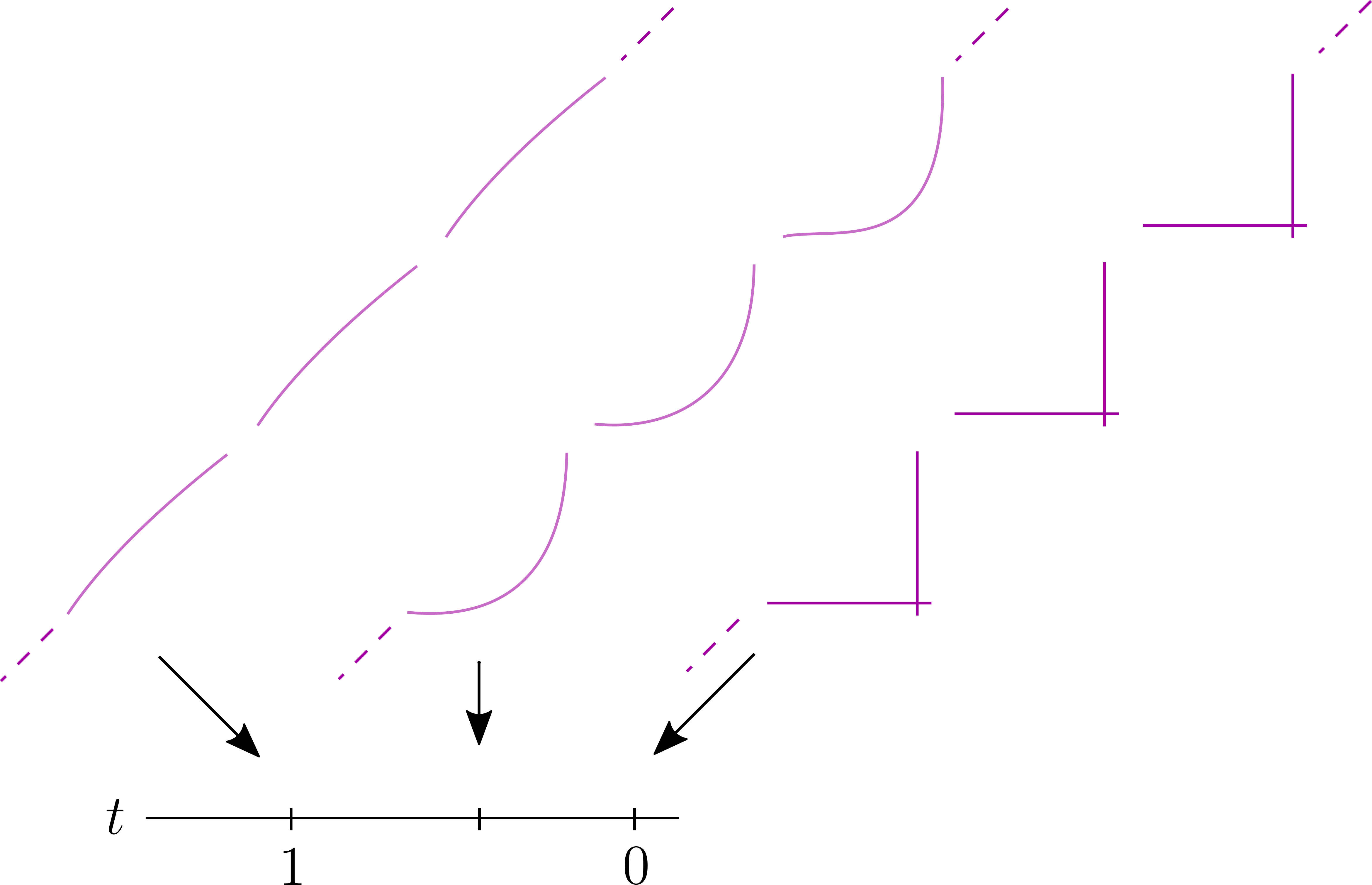
This is a symplectic fibration over punctured torus $T_{0}=T^{2}\setminus\{*\}$ with monodromy as shown in Figure 1.1. It can be shown to carry a Liouville structure and its contact boundary at infinity is isomorphic to that of $T_{0}\times M$, in other words the boundary of the mapping torus of identity.

One would like to distinguish the fillings $T_{\phi}$ and $T_{0}\times M$, when $\phi$ is not Hamiltonian isotopic to identity. An attempt can be made as follows: Assume the fillings are the same. Consider the partial compactification

Assume we are able to identify $\overline{T}_{\phi}$ with $\overline{T}_{1_{M}}=T^{2}\times M$. Every circle action on $T^{2}$ lifts to a circle action on $T^{2}\times M$; however, this is not the case with $\overline{T}_{\phi}$. Indeed, the flow of the obvious lift of $\partial_{t}$ at time $t=1$ gives us the symplectomorphism

which is different from the identity. In other words, it seems there are “more circle actions” on $T^{2}\times M$ and its flux group is bigger. The first and major limitation of this approach is our inability to identify the partial compactifications. Second limitation is even if one successfully runs the above program and rigorously computes the flux groups, they would only be able to conclude fiberwise $\phi$, the inverse of the symplectomorphism (1.3), is Hamiltonian isotopic to identity. We do not know how to conclude the same for $\phi$ acting on $M$.

One can instead try to follow an algebraic counterpart of the same idea, namely by executing this procedure at the level of Fukaya categories. By [Sei02], a compactification of a symplectic manifold by adding a divisor gives rise to a deformation of its Fukaya category, called the relative Fukaya category. For instance, by [LP12], the (compact) Fukaya category of the punctured torus $T_{0}$ is derived equivalent to the perfect complexes over the nodal elliptic curve $\mathcal{T}_{0}$, and the relative Fukaya category corresponding to partial compactification $T_{0}\subset T^{2}$ is equivalent to perfect complexes over the Tate family, which deforms $\mathcal{T}_{0}$. “The generic fiber” of this deformation is equivalent to Fukaya category of $T^{2}$. Therefore, instead of considering partial compactifications of $T_{\phi}$, one can consider deformations of its Fukaya category, which admit a classification in terms of invariants such as Hochschild cohomology. In the example above, the category corresponding to $T_{0}\subset T^{2}$ is essentially the unique deformation of the Fukaya category of $T_{0}$. One then runs a categorical incarnation of the dynamical idea above that goes back to [Sei14]. Namely, instead of counting circle actions on the manifold, one counts periodic “flow lines” on its Fukaya category. A periodic flow line is a family of derived equivalences of the category. Since derived equivalences are realized as convolution with an invertible bimodule (its “Fourier-Mukai kernel”), one can instead consider periodic families of invertible bimodules. Seidel [Sei14], makes this notion precise and considers such families parametrized by elliptic curves as a categorical replacement for the circle actions.

We run a similar idea on the Fukaya category of $T_{\phi}$. Fukaya category associated to a symplectic manifold is a category whose objects consist of Lagrangian manifolds. It is hard to construct interesting compact Lagrangians in $T_{\phi}$; for instance, if there are no $\phi$-invariant Lagrangians in $M$, then one does not have a Lagrangian in $T_{\phi}$ that is fibered over a longitude of the torus in Figure 1.3. On the other hand, for any Lagrangian $L\subset M$ and any open arc $\ell\subset T_{0}$, one can construct a Lagrangian in $T_{\phi}$ fibered over $\ell$ and has fiber $L$, but this Lagrangian is non-compact. As a result, one needs to consider the version of Fukaya categories that contain non-compact Lagrangians as well, called the wrapped Fukaya category $\mathcal{W}(T_{\phi})$ of $T_{\phi}$. Another advantage of working with wrapped Fukaya categories is the strong properties they satisfy, such as homological smoothness. Note that one does not have an analogue of the relative Fukaya category for wrapped Fukaya categories. However, we will take this as heuristic and work with deformations of the category directly.

Computations with Fukaya categories can be challenging. For instance, algebro-geometric machinery for deformation theory computations is not available. Taking homological mirror symmetry as the guiding principle, we give a semi-algebro geometric description of the wrapped Fukaya category of $T_{\phi}$, which simplifies various computations, construction of explicit deformations, as well as families of bimodules over the deformations, which we see as the categorical flow lines. More precisely, we describe the wrapped Fukaya category of $T_{\phi}$ in terms of the wrapped Fukaya category of $M$ and the action of $\phi$ on the category. The construction is very general: to every $A_{\infty}$-category $\mathcal{A}$ and auto-equivalence– still denoted by $\phi$– we associate a category $M_{\phi}$, called the mapping torus category of $\phi$. The goal of this paper is to run the program above in purely algebraic terms to distinguish $M_{\phi}$ from $M_{1_{\mathcal{A}}}$, the mapping torus of the identity, under various assumptions on $\mathcal{A}$. Note that $M_{\phi}$ will be a category “over $D^{b}(Coh(\mathcal{T}_{0}))$”, rather than $Perf(\mathcal{T}_{0})$, mirroring the use of non-compact Lagrangians.

An heuristic picture of the mapping torus category from algebraic geometry is as follows: given variety $X$ and automorphism $\phi_{X}$, one can construct an algebraic space by taking the product $\mathbb{P}^{1}\times X$ and gluing $\{0\}\times X$ to $\{\infty\}\times X$ after twisting by $\phi_{X}$ (i.e. by identifying $(0,x)$ with $(\infty,\phi_{X}(x))$ for all $x\in X$). This is a fibration over the nodal elliptic curve $\mathcal{T}_{0}$, and deforms compatibly with Tate family deforming $\mathcal{T}_{0}$. This deformation can be thought as the mirror analogue of the partial compactification $T_{\phi}\subset\overline{T}_{\phi}$. The generic fiber of this deformation is a rigid analytic mapping torus fibered over the generic fiber of the Tate family. For instance, when $\phi_{X}=1_{X}$, this is the product of an elliptic curve with $X$ (after appropriate base change). One has an analytic $\mathbb{G}_{m}$-action on the rigid analytic mapping torus, and it is periodic for $1_{X}$, whereas it is either non-periodic or has a larger period for other $\phi_{X}$. In other words, trivial mapping torus has more periodic actions, and this lets one to distinguish the non-trivial and trivial mapping tori. It is clear that before the deformation, there is no periodic action, as $\mathcal{T}_{0}$ is singular. Hence, one has to pass to this deformation, analogous to one’s need to pass to partial compactification of $T_{\phi}$ to see any circle actions. This is the mirror analogue of the above program. We categorify this idea to distinguish $M_{\phi}$ from $M_{1_{\mathcal{A}}}$. In other words, we construct deformation of these categories over the formal disc. Algebraic computations allow us to classify this deformation as the unique one that is non-trivial in the first order.

As mentioned, the idea to use “periodic flow lines” to distinguish Fukaya categories of symplectic manifolds is introduced in [Sei14]. There the author uses the “categorical flux” to distinguish Fukaya categories of compact mapping tori (similar to $\overline{T}_{\phi}$), as well as some related manifolds that could not be distinguished by other means. There are some differences between [Sei14] and our work: for instance, in our case, the periodic dynamics is broken for $M_{\phi}$ itself, but is only recovered once we pass to deformations. Another difference is that in [Sei14], the author does not construct “flow lines” and check if they are periodic. Instead, he realizes ”periodic flow lines” as families parametrized by elliptic curves, where the elliptic curve is allowed to vary. In our case, we construct families parametrized by a formal model for an annulus in the analytic multiplicative group $\mathbb{G}_{m}^{an}$, i.e. by a formal scheme whose generic fiber is the annulus in $\mathbb{G}_{m}^{an}$. Therefore, as we characterize families up to changes in the special fiber, they can actually be thought as families parametrized by (an annulus in) the analytic multiplicative group. Another difference between [Sei14] and the present work, at a more technical level, is the non-properness of the categories we consider. The tools introduced in [Sei14] are for proper categories; more precisely, this is needed to show the uniqueness of “flow lines”. We go around this problem by assuming the input category $\mathcal{A}$, despite being non-proper, is proper in each degree. This implies the same for $M_{\phi}$.

Let $\mathcal{A}$ be an $A_{\infty}$-category over $\mathbb{C}$ and $\phi$ be an auto-equivalence, i.e. an $A_{\infty}$-functor $\phi:\mathcal{A}\rightarrow\mathcal{A}$ such that $H^{*}(\phi):H^{*}(\mathcal{A})\rightarrow H^{*}(\mathcal{A})$ is an equivalence. For simplicity assume $\mathcal{A}$ is a dg category and $\phi$ is a dg functor acting bijectively on objects and hom-complexes of $\mathcal{A}$. Based on this, we construct an $A_{\infty}$ category $M_{\phi}$ over $\mathbb{C}$, and we call it the mapping torus category of $\phi$.

Briefly, the construction goes as follows. Consider the universal cover of the Tate curve $\tilde{\mathcal{T}}_{0}$ whose definition will be recalled in Section 2.1 (also see Figure 1.2). It is a nodal infinite chain of projective lines parametrized by $i\in\mathbb{Z}$, and it admits a translation automorphism $\mathfrak{tr}$ which moves one projective line to the next. Consider the bounded derived category of coherent sheaves supported on finitely many projective lines, denoted by $D^{b}(Coh_{p}(\tilde{\mathcal{T}}_{0}))$. We will construct a dg category $\mathcal{O}(\tilde{\mathcal{T}}_{0})_{dg}$ whose triangulated envelope is a dg enhancement of $D^{b}(Coh_{p}(\tilde{\mathcal{T}}_{0}))$. Moreover, it admits a strict dg autoequivalence, still denoted by $\mathfrak{tr}$, which lifts $\mathfrak{tr}_{*}$. Then, $\mathfrak{tr}\otimes\phi$ endows $\mathcal{O}(\tilde{\mathcal{T}}_{0})_{dg}\otimes\mathcal{A}$ with a $\mathbb{Z}$-action, and we define the mapping torus category as

The smash product with $\mathbb{Z}$, whose definition will be recalled in Section 4, corresponds geometrically to taking the quotient by the $\mathbb{Z}$-action.

The following example justifies the terminology “mapping torus category” from an algebro-geometric perspective:

We will assume the following conditions hold throughout the paper:

1. C.1

   $\mathcal{A}$ is (homologically) smooth, see [KS09] for a definition

2. C.2

   $\mathcal{A}$ is proper in each degree and bounded below, i.e. $H^{*}(hom_{\mathcal{A}}(x,y))=0$ is finite dimensional in each degree and vanishes for $*\ll 0$ for any $x,y\in Ob(\mathcal{A})$

3. C.3

   $HH^{i}(\mathcal{A})$, the $i^{th}$ Hochschild cohomology group of $\mathcal{A}$, is $0$ for $i<0$ and is isomorphic to $\mathbb{C}$ for $i=0$

Based on this $M_{\phi}$ will be shown to satisfy C.1-C.3 as well.

Now we can state our main theorem:

The proof goes as follows. Assume $M_{\phi}$ is Morita equivalent to $M_{1_{\mathcal{A}}}$. The notion of Morita equivalence will be recalled later in Definition 6.28, but we remark that this is equivalent to equivalence of derived categories for $A_{\infty}$-categories over $\mathbb{C}$. To any categorical mapping torus one can associate a natural formal deformation (with curvature) over the topological local ring $R=\mathbb{C}[[q]]$. We denote this deformation by $M_{\phi}^{R}$ (resp. $M_{1_{\mathcal{A}}}^{R}$). Its explicit construction is as follows. There exists a natural smoothing of $\tilde{\mathcal{T}}_{0}$, denoted by $\tilde{\mathcal{T}}_{R}$ (see Figure 2.1). To this we associate a curved dg category, denoted by $\mathcal{O}(\tilde{\mathcal{T}}_{R})_{cdg}$, and then apply the same construction as (1.4) replacing $\mathcal{O}(\tilde{\mathcal{T}}_{0})_{dg}$ by $\mathcal{O}(\tilde{\mathcal{T}}_{R})_{cdg}$. The deformations $M_{\phi}^{R}$ and $M_{1_{\mathcal{A}}}^{R}$ have no a priori relation to the Morita equivalence; however, $HH^{2}(M_{\phi})\cong HH^{2}(M_{1_{\mathcal{A}}})\cong\mathbb{C}$, under the assumptions of the theorem and the construction. Hence, there is only one formal deformation that is non-trivial at first order (up to reparametrization). Thus, we may assume without loss of generality that the Morita equivalence deforms to a Morita equivalence between $M_{\phi}^{R}$ and $M_{1_{\mathcal{A}}}^{R}$.

$M_{\phi}^{R}$ (resp. $M_{\phi}$) carries a canonical $\mathbb{G}_{m}(R)$ (resp. $\mathbb{G}_{m}$)-action for which the infinitesimal action makes sense (i.e. one can differentiate the action, see Definition 6.41). Infinitesimal action gives a class $\gamma_{\phi}^{R}\in HH^{1}(M_{\phi}^{R})$ (resp. $\gamma_{\phi}\in HH^{1}(M_{\phi})$). The action can be considered as a family of $M_{\phi}^{R}$-bimodules which is parametrized by the formal spectrum of $\mathbb{C}[t,t^{-1}][[q]]$, and which “follows” the class $1\otimes\gamma_{\phi}^{R}$ along $t\partial_{t}$ direction. This family can be considered as a “short flow line” for $1\otimes\gamma_{\phi}^{R}$, and we extend it to a “longer flow line”, i.e. to a family over the formal spectrum of $\mathbb{C}[u,t][[q]]/(ut-q)$. This is the formal completion of $\{ut=0\}\subset\mathbb{A}^{2}_{\mathbb{C}}$ and contains the formal spectrum $Spf(\mathbb{C}[t,t^{-1}][[q]])$ as a formal open subscheme, where the inclusion is induced by $t\mapsto t,u\mapsto qt^{-1}$. See Figure 1.3.

To construct the extended family we consider a formal subscheme $\mathcal{G}_{R}\subset\tilde{\mathcal{T}}_{R}\times\tilde{\mathcal{T}}_{R}\times Spf(\mathbb{C}[u,t][[q]]/(ut-q))$ with the following properties:

1. (1)

   it is flat over $Spf(\mathbb{C}[u,t][[q]]/(ut-q))$

2. (2)

   it restricts to the graph of $\widehat{\mathbb{G}_{m,R}}$-action (see Remark 2.3) over the formal spectrum $Spf(\mathbb{C}[t,t^{-1}][[q]])$

3. (3)

   it restricts to graph of composition of the inverse action with backwards translation $\mathfrak{tr}^{-1}$ over $Spf(\mathbb{C}[u,u^{-1}][[q]])$

In particular, we obtain the diagonal over the $R$-point $t=1$ and the graph of backwards translation over $u=1$. We turn $\mathcal{G}_{R}$ into a family of bimodules over $M_{\phi}^{R}$ by defining an $\mathcal{O}(\tilde{\mathcal{T}}_{R})_{cdg}$-$\mathcal{O}(\tilde{\mathcal{T}}_{R})_{cdg}$-bimodule

and showing it naturally descends to $M_{\phi}^{R}=(\mathcal{O}(\tilde{\mathcal{T}}_{R})_{cdg}\otimes\mathcal{A})\#\mathbb{Z}$. After some other technical replacements, we obtain a family $\mathcal{G}_{R}^{sf}$ of bimodules over $M_{\phi}^{R}$ parametrized by $\mathbb{C}[u,t][[q]]/(ut-q)$ satisfying properties G.1-G.3 below for $\gamma=\gamma_{\phi}^{R}$ and which restricts to “fiberwise $\phi$” at $u=1$, i.e. to the bimodule corresponding to descent of auto-equivalence $1\otimes\phi$ on $\mathcal{O}(\tilde{\mathcal{T}}_{R})_{cdg}\otimes\mathcal{A}$ to $M_{\phi}^{R}$. Hence, if we can show families constructed in this way correspond to each other under the Morita equivalence between $M_{\phi}^{R}$ and $M_{1_{\mathcal{A}}}^{R}$, this would imply the triviality of “fiberwise $\phi$” and therefore triviality of $\phi$, finishing the proof of the theorem.

For this, we would first need to show the classes $\gamma_{\phi}^{R}$ and $\gamma_{1_{\mathcal{A}}}^{R}$ correspond to each other under the isomorphism $HH^{1}(M_{\phi}^{R})\cong HH^{1}(M_{1_{\mathcal{A}}}^{R})$ induced by the Morita equivalence. To achieve this, we prove in Section 7 that these classes fall into natural rank $2$ lattices inside $HH^{1}(M_{\phi}^{R})\cong\mathbb{C}^{2}$ resp. $HH^{1}(M_{1_{\mathcal{A}}}^{R})\cong\mathbb{C}^{2}$ that are matched by the Morita equivalence, and show in Section 8 that the symmetries of $M_{1_{\mathcal{A}}}^{R}$ induce $SL_{2}(\mathbb{Z})$ symmetry on the lattice. Hence, we can use these categorical symmetries to fix the initial Morita equivalence so that the classes $\gamma_{\phi}^{R}$ and $\gamma_{1_{\mathcal{A}}}^{R}$ match.

Given this result, one would only need to prove a general theorem that states once the class $\gamma$ is fixed, the family is uniquely characterized by the following axioms:

1. G.1

   The restriction $\mathfrak{M}|_{q=0}$ is coherent. This is equivalent to its representability by an object of $tw^{\pi}(\mathcal{B}_{0}\otimes\mathcal{B}_{0}^{op}\otimes``\mathcal{C}oh(A)")$. See Definition 6.8.

2. G.2

   The restriction $\mathfrak{M}|_{t=1}$ is isomorphic to the diagonal bimodule over $\mathcal{B}$.

3. G.3

   The family follows the class $1\otimes\gamma\in HH^{1}(\mathcal{B}^{e})$.

This is achieved in Theorem 9.1, namely we show that two families satisfying G.1-G.3 are quasi-isomorphic up to $q$-torsion. The proof of Theorem 9.1 relies on two things: the ideas in [Sei14], which we recall in Section 6.2, and the algebra/geometry of modules over $\mathbb{C}[u,t][[q]]/(ut-q)$ which carry connections along the derivation $t\partial_{t}-u\partial_{u}$. More explicitly, given two such family $\mathcal{G}_{1}$ and $\mathcal{G}_{2}$, we show the hom-complexes in the category of families involving them are chain complexes of $\mathbb{C}[u,t][[q]]/(ut-q)$-modules carrying such connections in each degree that commute with the differentials. Hence, degree $0$ homomorphisms in the cohomological category give rank $1$ modules with connection, and we show in Appendix A that such modules are free up to $q$-torsion. Following this line of ideas we prove the isomorphism $\mathcal{G}_{1}|_{t=1}\simeq\mathcal{G}_{2}|_{t=1}$ extends over $\mathbb{C}[u,t][[q]]/(ut-q)$ to an isomorphism up to $q$-torsion. This completes the proof.

Now, let us detail the moral idea given in Section 1.2 for the algebro-geometric minded reader. Consider the algebro-geometric torus given in Example 1.1. It has a natural deformation

which is a fibration over the formal smoothing $\mathcal{T}_{R}=\tilde{\mathcal{T}}_{R}/t\sim\mathfrak{tr}(t)$. Its generic fiber $\mathfrak{Y}_{\mathbb{C}((q))}$ (in the sense of Raynaud, see [Tem15, Section 5]) gives

a rigid analytic version of $\mathbb{C}^{*}\times X/(t,x)\sim(q_{0}t,\phi_{X}(x))$, where $|q_{0}|<1$. There is an action of $\mathbb{G}_{m,\mathbb{C}((q))}^{an}$ on this rigid analytic space; however, it descends to an action of the elliptic curve $\mathbb{G}_{m,\mathbb{C}((q))}^{an}/q$ if and only if $\phi_{X}=1_{X}$. In other words, the trivial mapping torus will be distinguished from the others in that the restriction of the graph of the action to $z=q\in\mathbb{G}_{m,\mathbb{C}((q))}^{an}$ is the diagonal of $\mathfrak{Y}_{\mathbb{C}((q))}$ while in general it is the graph of fiberwise $\phi_{X}$. This action can be thought as analogous to the flow of a vector field. The uniqueness of the family is an analogue of the uniqueness of the flow of a vector field. This is more explicit if we consider the philosophy of Raynaud and realize rigid analytic spaces as formal schemes over $R=\mathbb{C}[[q]]$ up to admissable blow-ups in the special fiber $q=0$. In particular, the family $\mathcal{G}_{R}^{sf}$ obtained from the graph

morally corresponds to such a degeneration of the graph of action, restricted to a smaller annulus in $\mathbb{G}_{m,\mathbb{C}((q))}^{an}$ afterwards.

In Sections 2 and 3 we review the construction of $\tilde{\mathcal{T}}_{0}$, $\tilde{\mathcal{T}}_{R}$, and present the dg model $\mathcal{O}(\tilde{\mathcal{T}}_{0})_{dg}$ and its deformation $\mathcal{O}(\tilde{\mathcal{T}}_{R})_{cdg}$. In Section 4 we review the smash products and define $M_{\phi}$ and $M_{\phi}^{R}$. Section 5 is dedicated to computation of Hochschild cohomology and its results will be referred in other computations later. In Section 6, we construct the family $\mathcal{G}_{R}^{sf}$ and prove it satisfies desired properties. This section also contains a brief review of families. Sections 7 and 8 provide us the statements we need to fix the image of $\gamma_{\phi}\in HH^{1}(M_{\phi})\cong\mathbb{C}^{2}$ under the Morita equivalence. In Section 7, we show that the classes that are obtained as the infinitesimal action of a $\mathbb{G}_{m}$ (resp. $\mathbb{G}_{m}(R)$)-action on $M_{\phi}$ (resp. $M_{\phi}^{R}$) form a copy of $\mathbb{Z}^{2}$ inside $HH^{1}(M_{\phi})$ (resp. $HH^{1}(M_{\phi}^{R})\cong R^{2}$) generated by basis elements. This “cocharacter lattice” is obviously preserved under Morita equivalences, and Section 8 provides us symmetries of the categories acting transitively on primitive elements of the lattice. In Section 9, we finally conclude the proof of uniqueness(up to $q$-torsion) of families satisfying G.1-G.3 and the proof of Theorem 1.4. In the final section, Section 10, we relate the growth rates of $rk(HH^{*}(M_{\phi}^{R},\Phi^{k}_{f}))$, where $\Phi^{k}_{f}$ is the bimodule kernel of fiberwise $\phi^{k}$, to growth rates for $\phi$. In Appendix A, we prove some results (such as freeness up to $q$-torsion) for finitely generated modules over $A_{R}=\mathbb{C}[u,t][[q]]/(ut-q)$ with connections along $t\partial_{t}-u\partial_{u}$.

In [Kar19], we show that $M_{\phi}$ is actually derived equivalent to $\mathcal{W}(T_{\phi})$ with a canonical grading. Using this we find pairs of Liouville manifolds that can be distinguished by Theorem 1.4, but that have the same topology, contact boundary, symplectic cohomology groups, etc. Indeed, these examples are obtained by attaching subcritical handles to $T_{\phi}$ and $T_{1_{M}}$. One can kill the first cohomology of $T_{\phi}$, resp. $T_{1_{M}}$ by this process without changing wrapped Fukaya category. Theorem 1.4 implies $\mathcal{W}(T_{\phi})$ and $\mathcal{W}(T_{0}\times M)$ -endowed with canonical gradings- are not derived equivalent (one can grade these categories in different ways, but after killing the first cohomology the grading is unique). Note vanishing of first cohomology implies that arguments involving flux cannot be used either.

We believe Theorem 1.4 can be generalized as follows:

This produces an infinite family of pairwise non-equivalent categories; therefore, by the results of [Kar19], an infinite family of pairwise non-symplectomorphic Liouville manifolds. To prove Conjecture Conjecture, one only needs to prove existence of families like $\mathcal{G}_{\phi}$ that follow different (primitive) classes in the natural rank $2$ lattice in $HH^{1}(M_{\phi}^{R})$. Then, one obtains “flow lines along any class in the rank two lattice”. More precisely, these are families parametrized by formal schemes possibly different from $Spf(A_{R})$ (it is $Spf(A_{R})$ when the class is primitive in the lattice, note we do not define families with more general bases). The order of $\phi$ would be the index of the subgroup of the lattice given by the elements for which the restriction of the corresponding flow line to “other end” is the diagonal. More concretely, given $\gamma=k\gamma_{0}$, where $\gamma_{0}$ is a primitive class, construct a family parametrized by $Spf(A_{R})$ that follow $\gamma_{0}$ and that restrict to diagonal at $t=1$ and to $\Psi_{1}$ at $u=1$. Inductively construct a family parametrized by $A_{R}$ that follow $\gamma_{0}$ and that restricts to $\Psi_{1}$ at $t=1$ and to $\Psi_{2}$ at $u=1$, …, a family that restricts to $\Psi_{k-1}$ at $t=1$ and to $\Psi_{k}$ at $u=1$. Then, the elements $k\gamma_{0}$ such that $\Psi_{k}$ is quasi-isomorphic to diagonal bimodule form a subgroup of the lattice whose index is given by the order of $\phi$. This subgroup is intrinsic to $M_{\phi}$ and should be thought as an analogue of the flux group.

A generalization in an orthogonal direction is the following: one can construct a version of open symplectic mapping torus for two commuting symplectomorphisms: namely, given $\phi$ and $\psi$ acting on $M$, construct $T_{\phi,\psi}$ as the quotient of $(M\times\mathbb{R}\times\mathbb{R})\setminus(M\times\mathbb{Z}\times\mathbb{Z})$ by the relations

This generalizes $T_{\phi}$ and it still carries the structure of a symplectic fibration over $T_{0}=T^{2}\setminus\{*\}$ with non-trivial monodromy in both $\partial_{t}$ and $\partial_{s}$ directions. One can easily produce an analogous algebraic model for this construction. First build a model for the doubly infinite cover $(\mathbb{R}\times\mathbb{R})\setminus(\mathbb{Z}\times\mathbb{Z})\to T_{0}$ as follows: $\mathcal{O}(\tilde{\mathcal{T}}_{0})_{dg}$ contains a non-full quasi-equivalent subcategory $\mathcal{O}(\tilde{\mathcal{T}}_{0})_{dg}^{eval}$, on which the $\mathbb{G}_{m}$-action is rational. Consider the category $\tilde{\tilde{\mathcal{O}}}$ whose objects are given as the pairs $(\mathcal{F},i)$, where $\mathcal{F}\in ob(\mathcal{O}(\tilde{\mathcal{T}}_{0})_{dg})$ and $i\in\mathbb{Z}$. Let $\tilde{\tilde{\mathcal{O}}}((\mathcal{F},i),(\mathcal{F}^{\prime},i^{\prime}))$ be defined as the weight $i^{\prime}-i$ part of $\mathcal{O}(\tilde{\mathcal{T}}_{0})_{dg}^{eval}(\mathcal{F},\mathcal{F}^{\prime})$ with respect to the rational $\mathbb{G}_{m}$-action. This category carries a strict action of $\mathbb{Z}\times\mathbb{Z}$, where the first action is induced by $\mathfrak{tr}$ and the second by $(L,i)\mapsto(L,i+1)$. Clearly, $\tilde{\tilde{\mathcal{O}}}\#\mathbb{Z}$ (for the second $\mathbb{Z}$-action) is equivalent to $\mathcal{O}(\tilde{\mathcal{T}}_{0})_{dg}^{eval}$ (hence to $\mathcal{O}(\tilde{\mathcal{T}}_{0})_{dg}$). Then, given $\mathcal{A}$ as before with strictly commuting strict dg auto-equivalences $\phi$ and $\psi$, define $M_{\phi,\psi}$ to be $(\tilde{\tilde{\mathcal{O}}}\otimes\mathcal{A})\#(\mathbb{Z}\times\mathbb{Z})$. We expect this category to be equivalent to $\mathcal{W}(T_{\phi,\psi})$ with a canonical grading. We believe the following generalization of Theorem 1.4 and Conjecture Conjecture holds:

The intuition for this conjecture is similar. We believe this conjecture can be proven using similar steps, although we have not checked this.

One can also consider the category $M_{\phi[m],[n]}$, where $[m]$ and $[n]$ are the shift functors. An easy version of Conjecture Conjecture would state that $M_{\phi[m],[n]}$ is not Morita equivalent to $M_{[m^{\prime}],[n^{\prime}]}$, unless $\phi$ is quasi-isomorphic to a shift functor itself. Indeed, such a result can presumably be proven applying the results of this paper. First, observe $M_{\phi[m],[n]}$ can be obtained from $M_{\phi}$ by modifying the grading. Therefore, the same holds for Hochschild cohomology groups and in particular, one can show that $HH^{*}(M_{\phi[m],[n]})$ remains the same. One can attempt to construct a family following the class corresponding to $\gamma_{\phi}$ via change of grading. $\mathbb{G}_{m}\times\mathbb{G}_{m}$ still acts on $M_{\phi[m],[n]}$, and there exists a rank $2$ lattice consisting of classes followed by cocharacters of this action, as in Section 7. The action of $SL_{2}(\mathbb{Z})$-elements on $M_{1_{\mathcal{A}}}$ (see the action constructed in Section 8) turn into isomorphisms of $M_{[m^{\prime}],[n^{\prime}]}$ and $M_{[m^{\prime\prime}],[n^{\prime\prime}]}$, for when $gcd(m,n)=gcd(m^{\prime},n^{\prime})$ (i.e. when they are in the same $SL_{2}(\mathbb{Z})$-orbit). Hence, starting with a Morita equivalence $M_{\phi[m],[n]}\simeq M_{[m^{\prime}],[n^{\prime}]}$, one can switch to a Morita equivalence with $M_{[m^{\prime\prime}],[n^{\prime\prime}]}$ that preserves the canonical first Hochschild cohomology class. Their deformations match as before, and the families following degree $1$ classes also match again. The same argument works, but this time only to conclude that $\phi$ is equivalent to a shift functor. The importance of this generalization is that one obtains all possible gradings of $\mathcal{W}(T_{\phi})$ by changing $[m]$ and $[n]$; therefore, proving that $T_{0}\times M$ and $T_{\phi}$ are not symplectomorphic (as opposed to graded symplectomorphic, note grading becomes canonical after some subcritical handle attachment, i.e. one concludes that handle attached manifolds are not symplectomorphic without any need to use this generalization).

$R$ will always denote $\mathbb{C}[[q]]$ with the $q$-adic topology. Similarly, $A_{R}=\mathbb{C}[u,t][[q]]/(ut-q)$ with the $q$-adic topology and $A=\mathbb{C}[u,t]/(ut)=A_{R}/(q)$. $Spf(B)$ denotes the formal spectrum of a complete topological ring $B$ equipped with $I$-adic topology for an ideal $I\subset B$. This is a ringed space whose underlying topological space is $Spec(B/I)$(which is homeomorphic to $Spec(B/I^{m})$ for any $m>0$) and whose ring of global functions is the topological ring $\lim\limits_{\longleftarrow}B/I^{n}$. For more details see [Bos14]. Note, in our paper most formal affine schemes are completions of varieties along a closed subvariety.

Constructions/concepts over $R=\mathbb{C}[[q]]$ are implicitly assumed to be $q$-adically completed and continuous. This applies to categories over $R$, Hochschild cochains $CC^{*}(\mathcal{B})$ of such categories, and to tensor products of topological complete modules over $R$. For instance if $M$ and $N$ are such modules, $M\otimes N$ refers to $M\hat{\otimes}_{R}N$, which is the $q$-adic completion of $M\otimes N$. If $M$ is over $R$ and $N$ is over $\mathbb{C}$, $M\otimes N$ refers to $q$-adic completion of $M\otimes_{\mathbb{C}}N$. We also mostly drop the subscripts of tensor products from the notation. Similarly, the base of products of schemes or formal schemes are written only when it is unclear (for instance $\tilde{\mathcal{T}}_{R}\times\tilde{\mathcal{T}}_{R}$ refers to fiber product over $Spf(R)$).

We have elaborated on the definition of $\tilde{\mathcal{T}}_{0}$ in Section 2 (see also Figure 2.1). Indeed one can take

as the definition. For an explicit equation defining $\mathcal{T}_{0}$, see [LP12].

Given an ordinary algebra $B$, $\mathcal{C}_{dg}(B)$ denotes the dg category of chain complexes over $B$.

Given dg categories $\mathcal{B}$ and $\mathcal{B}^{\prime}$, we can their tensor product category as a category with objects $Ob(\mathcal{B})\times Ob(\mathcal{B}^{\prime})$. Let $b\times b^{\prime}$ denote the corresponding object of $\mathcal{B}\otimes\mathcal{B}^{\prime}$ for given $b\in Ob(\mathcal{B}),b^{\prime}\in Ob(\mathcal{B}^{\prime})$. Morphisms satisfy

See [Kel06] for more details.

For a given $A_{\infty}$-category $\mathcal{B}$, $tw(\mathcal{B})$ stands for the category of twisted complexes over $\mathcal{B}$ and $tw^{\pi}(\mathcal{B})$ stands for the split-closure (a.k.a. idempotent completion) of $tw(\mathcal{B})$. For a definition see [Sei08b, Chapter I.3,I.4]. $D^{\pi}(\mathcal{B})$ stands for the triangulated category $H^{0}(tw^{\pi}(\mathcal{B}))$. A dg/$A_{\infty}$ enhancement of a triangulated category $D$ is a dg/$A_{\infty}$ category $\mathcal{B}$ such that $D$ is equivalent to $H^{0}(\mathcal{B})$ as a triangulated category.

By generation, we mean split generation unless specified otherwise. See [Sei08b, Chapter I.4]. We used the notations $CC^{*}(\mathcal{B})$ and $CC^{*}(\mathcal{B},\mathcal{B})$ interchangeably. They both stand for the Hochschild complex of an $A_{\infty}$-category $\mathcal{B}$. See [Sei15], [Sei13]. The notation $Bimod(\mathcal{B},\mathcal{B}^{\prime})$ is used to mean the dg category of $A_{\infty}$-bimodules over $\mathcal{B}$-$\mathcal{B}^{\prime}$. There is a functor

which is naturally quasi-isomorphic to Yoneda functor of the diagonal bimodule. In the case of an $A_{\infty}$-algebra over $\mathbb{C}$, $CC^{*}(\mathcal{B},\mathfrak{M})$ has underlying graded vector space $\bigoplus_{i\geq 0}hom_{\mathbb{C}}(\mathcal{B}^{\otimes i},\mathfrak{M})[-i]=hom_{\mathbb{C}}(T\mathcal{B}[1],\mathfrak{M})$, where $T\mathcal{B}[1]=\bigoplus_{i\geq 0}\mathcal{B}^{\otimes i}[i]$(which is also defined in Section 6). We note that this direct sum means each degree of each summand is summed separately. Also, as remarked before the constructions take place in the category of completed $R$-modules in the case $\mathcal{B}$ is a curved category over $R$. For instance, $hom(\mathcal{B}^{\otimes i},\mathfrak{M})$ only involves convergent sums of continuous homomorphisms and direct sums are assumed to be $q$-adically completed. For the differential of $CC^{*}(\mathcal{B},\mathfrak{M})$, which involves $\mu_{\mathcal{B}}$ and $\mu_{\mathfrak{M}}$, see [Sei13, Remark 9.2].

For more homological algebra preliminaries see [Kel06], [Sei15],[Sei08b], [Sei13].

I would like to first thank to my advisor Paul Seidel, who introduced me to this problem and without his guidance this work would not be possible. I would also like to thank Padmavathi Srinivasan for illuminating conversations on the Tate curve and Neron models, to Yank$\char 16\relax$ Lekili for conversations on their work [LP12] and [LP16] and to Dhruv Ranganathan for conversations on the Tate curve as a rigid model for $\mathbb{G}_{m,K}^{an}$. Finally, I would like to thank the referee for reading the paper, and useful suggestions. This work was partially supported by NSF grant DMS-1500954 and by the Simons Foundation (through a Simons Investigator award).

We first review the construction of $\tilde{\mathcal{T}}_{R}$ following [LP12]. We slightly change the notation. Recall $R=\mathbb{C}[[q]]$ endowed with $q$-adic topology.

Given $i\in\mathbb{Z}$, let $\bar{U}_{i+1/2}$ denote $Spec\big(\mathbb{C}[q][X_{i},Y_{i+1}]/(X_{i}Y_{i+1}-q)\big)$. It is a scheme over $Spec(\mathbb{C}[q])$, and it is isomorphic to $\mathbb{A}^{2}_{\mathbb{C}}$ as a scheme over $\mathbb{C}$. Moreover,

is isomorphic to

as a scheme over $\mathbb{C}[q]$. Denote this scheme by $\bar{V}_{i}.$ The isomorphism is given by the coordinate change $X_{i}\leftrightarrow Y_{i}^{-1}$. In other words, the coordinates $X_{i}$ and $Y_{i}$ satisfy $X_{i}Y_{i}=1$ on $\bar{V}_{i}$.

By using the identifications $\bar{U}_{i+1/2}[X_{i}^{-1}]\cong\bar{U}_{i-1/2}[Y_{i}^{-1}]$, we can glue $\bar{U}_{i+1/2}$, $i\in\mathbb{Z}$. Hence, we obtain a scheme over $Spec(\mathbb{C}[q])$, which we denote by $\tilde{\mathcal{T}}_{\mathbb{C}[q]}$. It is not Noetherian and it is covered by charts $\bar{U}_{i+1/2}$, $i\in\mathbb{Z}$.

Note, there is a $\mathbb{G}_{m,\mathbb{C}[q]}$-action over $\mathbb{C}[q]$ on this scheme. Locally, the action is given by

where $t$ is the coordinate of $\mathbb{G}_{m,\mathbb{C}[q]}$.

We will mainly be interested in

and its formal completion inside $\tilde{\mathcal{T}}_{\mathbb{C}[q]}$. We denote this formal completion by

where the fiber product is taken with respect to the obvious morphism

(recall that $Spf(R)$ denotes the formal spectrum of the topological ring $R=\mathbb{C}[[q]]$).

Let $U_{i+1/2}:=\bar{U}_{i+1/2}|_{q=0}$ and $\tilde{U}_{i+1/2}:=\bar{U}_{i+1/2}\times_{Spec(\mathbb{C}[q])}Spf(\mathbb{C}[[q]])$. In the coordinates above,

and

respectively. In the latter, the formal spectrum is taken with respect to $q$-adic topology. Let

References

• [Abo10] Mohammed Abouzaid. A geometric criterion for generating the Fukaya category. Publ. Math. Inst. Hautes Études Sci., (112):191–240, 2010.
• [AG15] D. Arinkin and D. Gaitsgory. Singular support of coherent sheaves and the geometric Langlands conjecture. Selecta Math. (N.S.), 21(1):1–199, 2015.
• [AL17] Rina Anno and Timothy Logvinenko. Spherical DG-functors. J. Eur. Math. Soc. (JEMS), 19(9):2577–2656, 2017.
• [AM69] M. F. Atiyah and I. G. Macdonald. Introduction to commutative algebra. Addison-Wesley Publishing Co., Reading, Mass.-London-Don Mills, Ont., 1969.
• [Bos14] Siegfried Bosch. Lectures on formal and rigid geometry, volume 2105 of Lecture Notes in Mathematics. Springer, Cham, 2014.
• [Cha60] Stephen U. Chase. Direct products of modules. Trans. Amer. Math. Soc., 97:457–473, 1960.
• [Eis95] David Eisenbud. Commutative algebra, volume 150 of Graduate Texts in Mathematics. Springer-Verlag, New York, 1995. With a view toward algebraic geometry.
• [Fn07] Christian Frø nsdal. Quantization on curves. Lett. Math. Phys., 79(2):109–129, 2007. With an appendix by Maxim Kontsevich.
• [Gai13] Dennis Gaitsgory. ind-coherent sheaves. Mosc. Math. J., 13(3):399–528, 553, 2013.
• [GL87] Mark Green and Robert Lazarsfeld. Deformation theory, generic vanishing theorems, and some conjectures of Enriques, Catanese and Beauville. Invent. Math., 90(2):389–407, 1987.
• [GPS17] Sheel Ganatra, John Pardon, and Vivek Shende. Covariantly functorial wrapped Floer theory on Liouville sectors. arXiv e-prints, page arXiv:1706.03152v3, June 2017.
• [GPS18] Sheel Ganatra, John Pardon, and Vivek Shende. Sectorial descent for wrapped Fukaya categories. arXiv e-prints, page arXiv:1809.03427v2, September 2018.
• [Har66] Robin Hartshorne. Residues and duality. Lecture notes of a seminar on the work of A. Grothendieck, given at Harvard 1963/64. With an appendix by P. Deligne. Lecture Notes in Mathematics, No. 20. Springer-Verlag, Berlin-New York, 1966.
• [Har77] Robin Hartshorne. Algebraic geometry. Springer-Verlag, New York-Heidelberg, 1977. Graduate Texts in Mathematics, No. 52.
• [hh] Saal Hardali (https://mathoverflow.net/users/22810/saal hardali). Are all formal schemes *really* ind-schemes? MathOverflow. URL:https://mathoverflow.net/q/236351 (version: 2016-04-16).
• [hs] Zoran Skoda (https://mathoverflow.net/users/35833/zoran skoda). Functorial point of view for formal schemes. MathOverflow. URL:https://mathoverflow.net/q/33079 (version: 2010-07-23).
• [Huy06] D. Huybrechts. Fourier-Mukai transforms in algebraic geometry. Oxford Mathematical Monographs. The Clarendon Press, Oxford University Press, Oxford, 2006.
• [Kar19] Yusuf Barış Kartal. Distinguishing open symplectic mapping tori via their wrapped Fukaya categories. arXiv e-prints, page arXiv:1907.01156, Jul 2019.
• [Kel04] Bernhard Keller. Hochschild cohomology and derived Picard groups. J. Pure Appl. Algebra, 190(1-3):177–196, 2004.
• [Kel05] Bernhard Keller. On triangulated orbit categories. Doc. Math., 10:551–581, 2005.
• [Kel06] Bernhard Keller. On differential graded categories. In International Congress of Mathematicians. Vol. II, pages 151–190. Eur. Math. Soc., Zürich, 2006.
• [KS09] M. Kontsevich and Y. Soibelman. Notes on A∞A_{\infty}-algebras, A∞A_{\infty}-categories and non-commutative geometry. In Homological mirror symmetry, volume 757 of Lecture Notes in Phys., pages 153–219. Springer, Berlin, 2009.
• [LM08] Volodymyr Lyubashenko and Oleksandr Manzyuk. Quotients of unital A∞A_{\infty}-categories. Theory Appl. Categ., 20:No. 13, 405–496, 2008.
• [LO06] Volodymyr Lyubashenko and Sergiy Ovsienko. A construction of quotient A∞A_{\infty}-categories. Homology Homotopy Appl., 8(2):157–203, 2006.
• [LP12] Yanki Lekili and Timothy Perutz. Arithmetic mirror symmetry for the 2-torus, 2012.
• [LP16] Yanki Lekili and Alexander Polishchuk. Arithmetic mirror symmetry for genus 1 curves with nn marked points, 2016.
• [LS16] Valery A. Lunts and Olaf M. Schnürer. New enhancements of derived categories of coherent sheaves and applications. J. Algebra, 446:203–274, 2016.
• [Lun10] Valery A. Lunts. Categorical resolution of singularities. J. Algebra, 323(10):2977–3003, 2010.
• [Man04] Marco Manetti. Lectures on deformations of complex manifolds (deformations from differential graded viewpoint). Rend. Mat. Appl. (7), 24(1):1–183, 2004.
• [Mar06] Martin Markl. Transferring A∞A_{\infty} (strongly homotopy associative) structures. Rend. Circ. Mat. Palermo (2) Suppl., (79):139–151, 2006.
• [Sei02] Paul Seidel. Fukaya categories and deformations. In Proceedings of the International Congress of Mathematicians, Vol. II (Beijing, 2002), pages 351–360. Higher Ed. Press, Beijing, 2002.
• [Sei08a] Paul Seidel. A∞A_{\infty}-subalgebras and natural transformations. Homology Homotopy Appl., 10(2):83–114, 2008.
• [Sei08b] Paul Seidel. Fukaya categories and Picard-Lefschetz theory. Zurich Lectures in Advanced Mathematics. European Mathematical Society (EMS), Zürich, 2008.
• [Sei13] Paul Seidel. Lectures on categorical dynamics and symplectic topology, 2013. URL: http://math.mit.edu/~seidel/937/lecture-notes.pdf. Last visited on 2017/08/30.
• [Sei14] Paul Seidel. Abstract analogues of flux as symplectic invariants. Mém. Soc. Math. Fr. (N.S.), (137):135, 2014.
• [Sei15] Paul Seidel. Homological mirror symmetry for the quartic surface. Mem. Amer. Math. Soc., 236(1116):vi+129, 2015.
• [Ser73] J.-P. Serre. A course in arithmetic. Springer-Verlag, New York-Heidelberg, 1973. Translated from the French, Graduate Texts in Mathematics, No. 7.
• [Spa88] N. Spaltenstein. Resolutions of unbounded complexes. Compositio Math., 65(2):121–154, 1988.
• [ST01] Paul Seidel and Richard Thomas. Braid group actions on derived categories of coherent sheaves. Duke Math. J., 108(1):37–108, 2001.
• [Sta17] The Stacks Project Authors. stacks project. http://stacks.math.columbia.edu, 2017.
• [Tem15] Michael Temkin. Introduction to Berkovich analytic spaces. In Berkovich spaces and applications, volume 2119 of Lecture Notes in Math., pages 3–66. Springer, Cham, 2015.
• [Tho79] R. W. Thomason. Homotopy colimits in the category of small categories. Math. Proc. Cambridge Philos. Soc., 85(1):91–109, 1979.