Physical properties and optical-infrared transmission spectrum of the giant planet XO-1 b
Abstract
We present ten high-precision light curves of four transits in the XO-1 planetary system, obtained using , , , redshifted H, and filters. We use these to measure the physical properties, orbital ephemeris, and a transmission spectrum of the planet covering the full optical wavelength range. We augment this with published HST/WFC3 observations to construct a transmission spectrum of the planet covering 0.37 to 1.65 m. Our best-fitting model to this spectrum is for a H2/He-rich atmosphere containing water (3.05 confidence), nitrogen-bearing molecules NH3 and HCN (1.5) and patchy cloud (1.3). We find that adding the optical to the near-infrared data does not lead to more precise constraints on the planetary atmosphere in this case. We conduct a detailed investigation into the effect of stellar limb darkening on our results, concluding that the choice of limb darkening law and coefficients is unimportant; such conclusions may not hold for other systems so should be reassessed for all high-quality datasets. The planet radius we measure in the -band is anomalously low and should be investigated with future observations at a higher spectral resolution. From the measured times of transit we determine an improved orbital ephemeris, calculate a lower limit on the modified stellar tidal quality factor of , and rule out a previously postulated sinusoidal variation in the transit times.
Keywords:
stars: planetary systems — planets and satellites: atmospheres — stars: fundamental parameters — stars: individual: XO-11 Introduction
| Telescope / | Date of | Start time | End time | Filter | Airmass | Moon | Aperture | Scatter | ||||
|---|---|---|---|---|---|---|---|---|---|---|---|---|
| instrument | first obs | (UT) | (UT) | (s) | (s) | illum. | radii (px) | (mmag) | ||||
| INT/WFC | 2010 04 27 | 23:56 | 03:33 | 95 | 100 | 30 | red. H | 1.29 1.00 1.01 | 0.995 | 25 40 60 | 2 | 0.63 |
| CAHA/BUSCA | 2012 05 07 | 22:34 | 03:56 | 107 | 120 | 61 | SDSS | 1.19 1.01 1.25 | 0.945 | 27 33 60 | 1 | 3.35 |
| CAHA/BUSCA | 2012 05 07 | 22:34 | 03:56 | 107 | 120 | 61 | SDSS | 1.19 1.01 1.25 | 0.945 | 30 40 70 | 1 | 0.76 |
| CAHA/BUSCA | 2012 05 07 | 22:34 | 03:56 | 107 | 120 | 61 | SDSS | 1.19 1.01 1.25 | 0.945 | 32 42 80 | 1 | 0.55 |
| CAHA/BUSCA | 2012 05 07 | 23:19 | 03:56 | 92 | 120 | 61 | SDSS | 1.10 1.01 1.25 | 0.945 | 30 40 70 | 1 | 0.75 |
| CAHA/BUSCA | 2012 05 11 | 21:35 | 03:58 | 142 | 100–120 | 52 | SDSS | 1.34 1.01 1.31 | 0.595 | 23 33 60 | 1 | 1.44 |
| CAHA/BUSCA | 2012 05 11 | 21:35 | 03:47 | 138 | 100–120 | 52 | SDSS | 1.34 1.01 1.27 | 0.595 | 30 40 70 | 1 | 0.64 |
| CAHA/BUSCA | 2012 05 11 | 21:35 | 03:58 | 147 | 100–120 | 52 | SDSS | 1.34 1.01 1.31 | 0.595 | 30 45 80 | 2 | 1.78 |
| CAHA/BUSCA | 2012 05 11 | 21:35 | 03:58 | 145 | 100–120 | 52 | SDSS | 1.34 1.01 1.31 | 0.595 | 25 40 80 | 2 | 0.72 |
| CAHA/1.23m | 2014 05 26 | 21:39 | 02:58 | 151 | 105–125 | 11 | Cousins | 1.15 1.01 1.30 | 0.036 | 30 45 80 | 1 | 0.61 |
The atmospheric properties of giant planets are an important indicator of the formation and evolution of planets and planetary systems (Madhusudhan et al., 2014; Mordasini et al., 2016). They are also observationally accessible in a large fraction of hot Jupiters (planets with mass 0.3 and orbital period 10 d) which transit their host star, via the method of transmission spectroscopy.
Transmission spectroscopy offers a way of measuring the radius of the planet as a function of wavelength, by determining the transit depth at multiple wavelengths. It is sensitive to the amount of absorption and scattering of starlight passing though the outer atmosphere of the planet whilst it is backlit by its host star. Transmission spectroscopy can be used to detect enhanced opacity due to atomic absorption, molecular absorption and Rayleigh scattering (Pont et al., 2013; Madhusudhan et al., 2014; Fischer et al., 2016, e.g.). This can yield constraints on the chemical composition of the atmosphere, its temperature-pressure structure, and the presence of cloud or haze particles. The first detection of the atmosphere of an extrasolar planet was due to sodium absorption in HD 209458 b (Charbonneau et al., 2002), and extensive results have recently been obtained from both the ground and space (Nikolov et al., 2016; Sing et al., 2016, e.g.).
In the near future the NASA James Webb Space Telescope (JWST) will revolutionise this research area with extensive observations covering wavelengths from 0.6 m to 28 m (Beichman et al., 2014; Greene et al., 2016). It is expected to be used to study a significant sample of planets, and by comparison to HST it will achieve much lower Poisson noise, more extensive wavelength intervals, and uninterrupted coverage of individual transits.
Stevenson et al. (2016) outlined an Early Release Science program intended to occur shortly after JWST enters service, in which extensive observations of a small number of transiting planets will be performed using multiple instruments and observing modes. The aims are to allow an assessment of the relative strengths of the observing modes, and to expedite the development of data reduction pipelines for this work. Stevenson et al. selected 12 transiting planets as promising targets. XO-1 is one of the most suitable targets within this list, with a sky position near the continuous viewing zone of JWST, a host star which is bright (; Skrutskie et al. 2006) and inactive (; Knutson et al. 2010), and a planet with an atmospheric scale height (277 km) suitable for obtaining transmission spectra with a significant signal to noise ratio. In this work we present a detailed analysis of the XO-1 system, based on new transit light curves in six optical passbands plus published infrared transmission spectroscopy, in order to measure the physical properties of the system, refine the orbital ephemeris, and investigate the atmospheric properties of the planet.
XO-1 was only the eleventh transiting extrasolar planet (TEP) discovered (McCullough et al., 2006), and was found to be a 0.92 and 1.21 planet orbiting a 1.04 and 0.94 G1 V star every 3.94 d (Southworth, 2010). Follow-up light curves from Holman et al. (2006) were analysed using homogeneous methods by both Torres et al. (2008) and Southworth (2008); Southworth (2009); Southworth (2011). Occultations (secondary eclipses) were observed by Machalek et al. (2008) using the Spitzer Space Telescope, from which flux ratios of the planet to the star were measured in the four IRAC passbands (3.6, 4.5, 5.8 and 8.0 m). Tinetti et al. (2010) and Burke et al. (2010) presented and studied HST/NICMOS transmission spectroscopy of XO-1 b, finding evidence for the presence of the molecules H2O, CH4 and CO2. Their results have been questioned by Gibson et al. (2011) based on a reanalysis of the same data, and by Deming et al. (2013) based on new HST/WFC3 transmission spectroscopy. Deming et al. found evidence for water in the transmission spectrum of XO-1 b, a conclusion also reached by Tsiaras et al. (2018).
In addition to the works cited above, transit light curves have been presented by Vaňko et al. (2009); Cáceres et al. (2009); Raetz et al. (2009) and Sada et al. (2012), spectroscopic analyses of the host star have been performed by Ammler-von Eiff et al. (2009); Torres et al. (2012); Mortier et al. (2013) and Teske et al. (2014), and the orbital eccentricity has been constrained to be less than 0.29 by Madhusudhan & Winn (2009) and Pont et al. (2011). Most recently, Bonomo et al. (2017) presented new radial velocity measurements from which they constrained the eccentricity to be less than 0.019 to and 0.043 to .
High-resolution imaging of TEP host stars is an important part of determining the physical properties of the system (Evans et al., 2016, e.g.). Lucky Imaging of the XO-1 system was presented by Wöllert et al. (2015), who found no nearby stars less than 3.97, 4.85, 5.79 and 6.46 mag fainter than XO-1 A (5 detection limits) in the band at distances of 0.25′′, 0.5′′, 1.0′′ and 2.0′′, respectively.
The outline of this paper is as follows. Section 2 presents our new observations of XO-1, which are analysed in Section 3 alongside published light curves. The results are used to measure the physical properties of the system in Section 4. Section 5 presents an improved orbital ephemeris and a search for transit timing variations. The transmission spectrum of XO-1 b is obtained and analysed in Section 6, after which the paper is concluded in Section 7.
2 Observations and data reduction
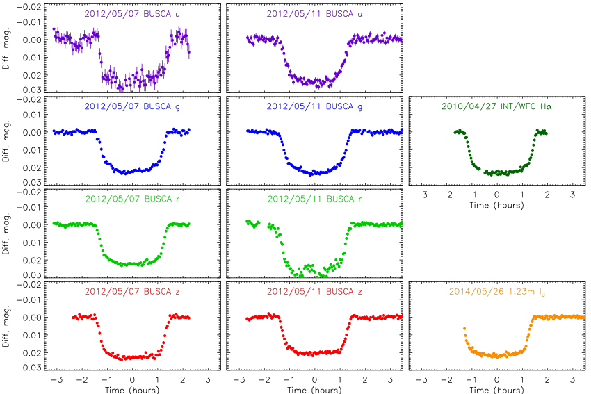
Two transits of XO-1 were observed using the BUSCA four-band imaging photometer on the 2.2 m telescope at Calar Alto, Spain. We selected Sloan , , and filters (Fukugita et al., 1996) from the Calar Alto filter database, which with BUSCA yield a circular field of view approximately 5.8′ in diameter. We were not able to obtain good photometry simultaneously in the bands with the lowest and highest counts ( and respectively), because the four arms of BUSCA cannot be operated at different focus levels or exposure times. We therefore optimised for the -band on the first night and the -band on the second night. The -band light curve from 2012/05/07 therefore has a large scatter due to low flux levels, and the - band light curve from 2012/05/11 displays systematic effects due to being near the saturation level of the CCD. An observing log is given in Table 1 and further details of our approach with BUSCA can be found in Southworth et al. (2012).
One transit of XO-1 was observed with the Isaac Newton Telescope (INT) and Wide Field Camera (WFC) on La Palma, Spain. We used CCD 4, as this is the one on the optical axis, and a redshifted H filter (ING filter11
1
http://catserver.ing.iac.es/filter/list.php?
instrument=WFC #226, central wavelength 689 nm, FWHM 10 nm) rather than a wide-band filter in order to limit the amount of defocussing used. We were not able to autoguide as the guide CCD is in the same focal plane as the science instrument.
One transit of XO-1 was obtained with the 1.23 m telescope at Calar Alto, using a Cousins filter. The transit ingress was missed due to technical problems, but the light curve is otherwise excellent.
The data were reduced using the defot pipeline (Southworth et al., 2009; Southworth et al., 2014), which depends on the NASA astrolib library22 2 http://idlastro.gsfc.nasa.gov/ idl33 3 http://www.harrisgeospatial.com/SoftwareTechnology/ IDL.aspx implementation of the aper routine from daophot (Stetson, 1987). Software apertures were placed by hand and their radii chosen to minimise the scatter in the final light curve. The apertures were shifted to account for telescope pointing wander, which was measured by cross-correlating each image with a reference image. We did not perform bias or flat-field calibrations as these had little effect on the final light curves beyond a slight increase in the scatter of the data.
A differential-magnitude light curve of XO-1 was generated for each observing sequence versus an ensemble comparison star containing the weighted flux sum of the good comparison stars. A polynomial was also fitted to the observations outside transit and subtracted to rectify the final light curve to zero differential magnitude. The order of the polynomial was chosen to be the lowest which gave a good fit to the out-of-transit data. The coefficients of the polynomial and the weights of the comparison stars were simultaneously optimised to minimise the scatter in the datapoints outside eclipse. The observational errors were then scaled so each transit had a reduced of versus a best-fitting model calculated with the jktebop code (see below). Table 1 includes the polynomial order and the of the residuals versus the best fit for each light curve. The final data are shown in Fig. 1 and listed in Table 2. The times given refer to the midpoint of the exposure on the BJD/TDB timescale (Eastman et al., 2010).
3 Light curve analysis
3.1 Approach
We modelled the available transit light curves of XO-1 using the jktebop44 4 jktebop is written in fortran77 and the source code is available at http://www.astro.keele.ac.uk/jkt/codes/jktebop.html code (Southworth, 2013, and references therein) and the formalism of the Homogeneous Studies project (see Southworth, 2012, and references therein). The fitted parameters were as follows.
- •
The sum and ratio of the fractional radii of the two components, and , where the fractional radii are the absolute radii in units of the semimajor axis: . These combinations of parameters were chosen because they are only weakly correlated.
- •
The orbital inclination, .
- •
A time of mid-transit, .
- •
The coefficients of a polynomial of differential magnitude versus time. The polynomial order for each light curve is given in Table 1. Whilst the fitted polynomials were removed at the data-reduction stage, their inclusion in the jktebop fit is necessary to propagate their uncertainties into the measured photometric parameters.
- •
One or two limb darkening (LD) coefficients, depending on the solution performed.
The orbital period was held fixed in each solution, because the uncertainty in its value was utterly negligible for this analysis. We also enforced orbital circularity in the absence of evidence for an eccentric orbit (Anderson et al., 2012, see discussion in).
| Telescope / | Filter | BJD(TDB) | Diff. mag. | Uncertainty |
|---|---|---|---|---|
| instrument | 2400000 | |||
| INT/WFC | rH | 55314.497407 | 0.0003821 | 0.0006442 |
| BUSCA | 56055.445999 | 0.0059505 | 0.0028984 | |
| BUSCA | 56055.445999 | 0.0006606 | 0.0007777 | |
| BUSCA | 56055.445999 | 0.0007141 | 0.0005374 | |
| BUSCA | 56055.477499 | 0.0002283 | 0.0007324 | |
| BUSCA | 56059.405206 | 0.0010300 | 0.0015896 | |
| BUSCA | 56059.405206 | 0.0006314 | 0.0006988 | |
| BUSCA | 56059.405206 | 0.0018004 | 0.0007984 | |
| BUSCA | 56059.405206 | 0.0008813 | 0.0008654 | |
| CAHA123 | 56804.408021 | 0.0063808 | 0.0005926 |
We performed jktebop solutions using each of four two-parameter LD ‘laws’: quadratic, square-root, logarithmic and cubic (Southworth, 2008, see). We furthermore calculated solutions with both LD coefficients fixed at theoretical values, the linear coefficient fitted and the nonlinear coefficient fixed, and both coefficients fitted. The theoretical LD coefficients were obtained by bilinearly interpolating55 5 Bilinear interpolation was performed using the jktld code at: http://www.astro.keele.ac.uk/jkt/codes/jktld.html in tabulated predictions to the host star’s measured effective temperature () and surface gravity (). We considered multiple sources of theoretical coefficients (Van Hamme, 1993; Claret, 2000; Claret & Hauschildt, 2003; Claret, 2004a) and averaged their predictions when necessary.
Least-squares best fits were obtained using the Levenberg-Marquardt method (Markquardt, 1963) as implemented in the mrqmin routine (Press et al., 1992). The uncertainties in the fitted parameters were estimated using both Monte Carlo and residual-permutation solutions (see Southworth, 2008, for further details), and the larger errorbar was retained for each measured parameter. Uncertainties were further inflated to account for any scatter in the measured values of a parameter from the solutions using different approaches to the inclusion of LD. Tables of results for each light curve can be found in the Supplementary Information. The measured photometric parameters are given in Table 3.
3.2 Our new data
| Source | (∘) | |||||||||
|---|---|---|---|---|---|---|---|---|---|---|
| BUSCA | 0.1048 | 0.0063 | 0.1372 | 0.0032 | 87.22 | 1.17 | 0.0923 | 0.0053 | 0.01253 | 0.00101 |
| BUSCA | 0.0993 | 0.0024 | 0.1289 | 0.0014 | 89.07 | 0.74 | 0.0880 | 0.0020 | 0.01133 | 0.00038 |
| BUSCA | 0.1002 | 0.0024 | 0.1331 | 0.0012 | 88.82 | 0.81 | 0.0884 | 0.0021 | 0.01177 | 0.00037 |
| BUSCA | 0.1014 | 0.0027 | 0.1327 | 0.0015 | 88.50 | 0.81 | 0.0895 | 0.0023 | 0.01188 | 0.00038 |
| INT/WFC rH | 0.0977 | 0.0015 | 0.1339 | 0.0027 | 89.88 | 0.62 | 0.0862 | 0.0013 | 0.01154 | 0.00022 |
| 1.23 m | 0.1012 | 0.0029 | 0.1334 | 0.0013 | 88.52 | 0.58 | 0.0893 | 0.0025 | 0.01191 | 0.00042 |
| Holman et al. (2006) FLWO | 0.1009 | 0.0023 | 0.1321 | 0.0012 | 88.56 | 0.66 | 0.0891 | 0.0019 | 0.01177 | 0.00033 |
| Holman et al. (2006) Palomar | 0.0953 | 0.0043 | 0.1265 | 0.0028 | 89.99 | 1.03 | 0.0846 | 0.0037 | 0.01070 | 0.00063 |
| Cáceres et al. (2009) SofI | 0.1018 | 0.0025 | 0.1324 | 0.0021 | 88.47 | 0.47 | 0.0899 | 0.0022 | 0.01191 | 0.00036 |
| Cáceres et al. (2009) ISAAC | 0.0978 | 0.0038 | 0.1321 | 0.0018 | 89.81 | 0.95 | 0.0863 | 0.0033 | 0.01140 | 0.00063 |
| Sada et al. (2012) | 0.1082 | 0.0110 | 0.1297 | 0.0063 | 87.92 | 1.86 | 0.0958 | 0.0092 | 0.01242 | 0.00176 |
| Final results | 0.0997 | 0.0008 | 0.1325 | 0.0008 | 88.84 | 0.22 | 0.0880 | 0.0007 | 0.01166 | 0.00012 |

The data from the two transits of XO-1 observed with BUSCA were collected into one light curve for each filter, and each was modelled with jktebop (see Fig. 2). We made two exceptions to this approach: the -band data from 2012/05/07 were ignored because the low flux levels caused a large scatter, and the -band data from 2012/05/11 were rejected because they suffer from saturation effects. We found that the -band light curves are in excellent agreement with each other ( when the individual light curves have ). However, the -band light curves are not (), as can be seen in Fig. 1. Our resulting parameters for the -band are therefore roughly the average for the two datasets, and are in fact in good agreement with the results from other light curves.
In all cases except BUSCA , we adopt the results from jktebop models with the linear LD coefficient fitted and the nonlinear LD coefficient fixed, as these agree very well both between different LD laws and between different datasets. For BUSCA we found that the data were unable to support fitting for even one LD coefficient, so we adopt the results obtained with both coefficients fixed. LD coefficients are not available for the redshifted H filter. We therefore used those for the Johnson filter, which has a similar central wavelength (0.67 m; Johnson 1964). The effect of the difference in passband on the LD coefficients is expected to be smaller than the intrinsic uncertainty of the coefficients, as judged from the variation in predictions for the same filters from different sources.
3.3 Reanalysis of published data

The literature for XO-1 includes several light curves of a quality sufficient for inclusion in the current work. We have obtained these data and modelled them using the same methods as for our own observations. The results are included in Table 3 and are discussed below.
Holman et al. (2006) presented light curves of two transits of XO-1 obtained with the FLWO 1.2 m telescope and KeplerCam in the -band, and one transit observed using the Palomar 1.5 m in the band. According to the webpage for this facility66
6
http://www.astro.caltech.edu/palomar/observer/
P60observers.html this corresponds to a Kron-Cousins band. Both datasets have been analysed in the past by the first author (Southworth, 2008) but were reanalysed with the modification that a first-order polynomial was applied to each transit, an option added to jktebop since the previous analysis (Southworth et al., 2014, see). The best fits are shown in Fig. 3 and were each obtained with one fitted and one fixed LD coefficient.
Cáceres et al. (2009) published observations of four transits of XO-1, all obtained at near-infrared wavelengths. We ignored their Run A due to the large systematic errors visible in the data, and their Run C due to the patches of very high scatter during transit. We therefore analysed their Run B, which was obtained using NTT/SofI in the -band, and their Run D, observed using VLT/ISAAC in the -band but with a blocking filter to remove flux from a red leak in the filter. Both runs were obtained at high cadence, with integration times of 0.8 s and 0.08 s respectively and very low dead times. We therefore binned the light curves by factors of 100 and 1000, respectively, to yield a sampling rate of approximately 80 s in both cases. Whereas the SofI data could be satisfactorily modelled with one fitted LD coefficient, we had to fix both to obtain an acceptable solution of the ISAAC observations. In both cases we included a second-order polynomial to model the baseline brightness of the system.
Sada et al. (2012) observed one transit in the -band using a 0.5 m telescope at Kitt Peak National Observatory. The ingress was missed and the data have an expectedly large scatter of 2.9 mmag, but we ran the usual jktebop solutions in order to determine whether this dataset can provide results worth including on our analysis. We allowed for a second-order polynomial baseline function.
3.4 Combined results

The measured photometric parameters are given in Table 3 and show a good agreement between light curves. We calculated the weighted mean value for each measured parameter for use in the next section. The value of the individual values versus the weighted mean is good for , and (0.6, 0.6 and 0.9, respectively) but less so for (1.8). This could be caused by residual systematic errors and/or by a true astrophysical signal (i.e. a non-flat transmission spectrum; see Southworth & Evans 2016). We have multiplied the uncertainty in the weighted mean of by to account for this.
Casual inspection of Table 3 suggests that correlations exist between several of the photometric parameters. Such correlations are widely known (Southworth, 2008; Pál, 2008; Carter et al., 2008, e.g.) and must be accounted for in the uncertainties of the parameter measurements. In Fig. 4 we illustrate two of these correlations: between and , and between and . The former arises because and together determine the duration of the transit (Seager & Mallén-Ornelas, 2003), and the latter occurs as is much better-determined than either or . It is clear from Fig. 4 that the correlations are greatly attenuated using the high-quality light curves presented here, and that the errorbars in Table 3 are not underestimated. For reference, the linear Pearson correlation coefficients are and , respectively.
4 Physical properties
References: (1) McCullough et al. (2006); (2) Ammler-von Eiff et al. (2009); (3) Torres et al. (2012); (4) Mortier et al. (2013); (5) Teske et al. (2014); (6) Brewer et al. (2016).
| (K) | (dex) | (c.g.s.) | Ref | |||
| 5750 | 13∗ | 0.015 | 0.040∗ | 4.53 | 0.065∗ | 1 |
| 5754 | 42 | 0.01 | 0.05 | 4.61 | 0.05 | 2 |
| 5738 | 65 | 0.06 | 0.05 | 4.50 | 0.01 | 3 |
| 5754 | 42 | 0.01 | 0.05 | 4.61 | 0.05 | 4 |
| 5695 | 26 | 0.11 | 0.06 | 4.42 | 0.12 | 5 |
| 5729 | 25∗ | 0.07 | 0.010∗ | 4.49 | 0.028∗ | 6 |
| Adopted parameters: | ||||||
| 5740 | 50 | 0.03 | 0.05 | |||
| Parameter | This work | Burke et al. (2010) | |||
| () | 1.018 | 0.028 | 0.034 | 1.027 | 0.06 |
| () | 0.930 | 0.011 | 0.010 | 0.94 | 0.02 |
| (cgs) | 4.509 | 0.009 | 0.005 | 4.50 | 0.01 |
| () | 1.23 | 0.03 | |||
| () | 0.907 | 0.022 | 0.020 | 0.92 | 0.08 |
| () | 1.199 | 0.017 | 0.013 | 1.21 | 0.03 |
| ( m s-2) | 15.5 | 1.1 | |||
| () | 0.492 | 0.018 | 0.005 | 0.48 | 0.04 |
| (K) | |||||
| (AU) | 0.04914 | 0.00045 | 0.00054 | 0.049 | 0.001 |
| Age (Gyr) | |||||
We used the results of the photometric analysis from the previous section to obtain the full physical properties of the system. This process also required knowledge of the spectroscopic properties of the host star (effective temperature and metallicity ) which are summarised in Table 4, and the stellar orbital velocity amplitude, m s-1 (Bonomo et al., 2017). As the necessary additional constraint, we used tabulated predictions from each one of five sets of theoretical stellar models (Claret, 2004b; Demarque et al., 2004; Pietrinferni et al., 2004; VandenBerg et al., 2006; Dotter et al., 2008).
We then estimated the value of the velocity amplitude of the planet, and calculated the physical properties of the system using this and the measured quantities. We iteratively adjusted to optimise the agreement between the calculated and the measured , and between the and that predicted by the stellar models for the observed and calculated stellar mass (). We did this for ages from 0.1 Gyr to 20 Gyr in steps of 0.1 Gyr, from which we identified the overall best fit and age of the system (Southworth, 2009, see). This process was undertaken for each of the five sets of tabulated theoretical model predictions, and the final parameters were taken to be the median of the five different possibilities arising from this repeated analysis.
We propagated the statistical errors in all input parameters using a perturbation analysis, and added all contributions in quadrature for each output parameter. We estimated the systematic uncertainties, which are incurred by the use of theoretical stellar models, by taking the maximum deviation between the final parameter value and the individual values obtained using the different sets of tabulated predictions.
The measured physical properties of the XO-1 system are given in Table 5. The mass, radius, gravity and density of the star are denoted by: , , and ; and of the planet by , , and , respectively. Our results are in good agreement with all previously published measurements. Our measured is equivalent to a relatively large stellar density, which means that the best-fitting theoretical star is near the zero-age main sequence. We therefore see a significant systematic uncertainty in our results caused by edge effects in the model tabulations, and by the intrinsic variation in how different stellar evolution codes initialise their stellar models. Table 5 also includes a comparison between our measurements and those of Burke et al. (2010), which are in very good agreement.
This young age is surprising because it is not supported by other age indicators such as chromospheric activity and rotational velocity. Knutson et al. (2010) observed the cores of the Ca II H & K lines, finding a small core emission due to stellar activity. They measured an activity index of , which indicates that it is a relatively inactive star. The calibration of Mamajek & Hillenbrand (2008) points to an age of roughly 6 Gyr with an uncertainty of perhaps 0.05 dex due to astrophysical scatter, and unknown uncertainties due to the value (which is not supplied with an errorbar) and activity cycles on XO-1 A (because we only have one measurement of ). One possible solution to this conflict is inaccuracies in theoretical models (Maxted et al., 2015, e.g.), with perhaps a small contribution from an orbital eccentricity which is large enough to affect the measured but small enough to hide in the available radial velocity measurements.
5 Transit timing analysis
| Time of minimum | Uncertainty | Cycle | Residual | Reference |
|---|---|---|---|---|
| (BJD/TDB) | (d) | number | (d) | |
| 2453127.03924 | 0.00580 | 555.0 | 0.00167 | Wilson et al. (2006) |
| 2453150.68624 | 0.01060 | 549.0 | 0.00036 | Wilson et al. (2006) |
| 2453154.62574 | 0.00260 | 548.0 | 0.00236 | Wilson et al. (2006) |
| 2453158.56704 | 0.00340 | 547.0 | 0.00257 | Wilson et al. (2006) |
| 2453162.51444 | 0.00250 | 546.0 | 0.00333 | Wilson et al. (2006) |
| 2453166.45124 | 0.00250 | 545.0 | 0.00138 | Wilson et al. (2006) |
| 2453170.39244 | 0.00370 | 544.0 | 0.00168 | Wilson et al. (2006) |
| 2453229.51504 | 0.00450 | 529.0 | 0.00165 | Wilson et al. (2006) |
| 2453237.40504 | 0.00320 | 527.0 | 0.00534 | Wilson et al. (2006) |
| 2453241.34174 | 0.00670 | 526.0 | 0.00054 | Wilson et al. (2006) |
| 2453808.91774 | 0.00110 | 382.0 | 0.00012 | McCullough et al. (2006) |
| 2453875.92321 | 0.00047 | 365.0 | 0.00023 | This work (Palomar data from Holman et al. 2006) |
| 2453879.86474 | 0.00110 | 364.0 | 0.00021 | Holman et al. (2006) |
| 2453883.80638 | 0.00018 | 363.0 | 0.00007 | This work (FLWO data from Holman et al. 2006) |
| 2453887.74746 | 0.00015 | 362.0 | 0.00049 | This work (FLWO data from Holman et al. 2006) |
| 2453887.74774 | 0.00060 | 362.0 | 0.00021 | B. Gary (AXA) |
| 2453911.39781 | 0.00049 | 356.0 | 0.00083 | J. Ohlert (TRESCA) |
| 2454171.53332 | 0.00170 | 290.0 | 0.00298 | Raetz et al. (2009) |
| 2454214.89274 | 0.00090 | 279.0 | 0.00011 | B. Gary (AXA) |
| 2454218.83405 | 0.00114 | 278.0 | 0.00030 | Cáceres et al. (2009) |
| 2454222.77623 | 0.00023 | 277.0 | 0.00037 | This work (SofI data from Cáceres et al. 2009) |
| 2454222.77671 | 0.00039 | 277.0 | 0.00085 | Cáceres et al. (2009) |
| 2454226.71808 | 0.00033 | 276.0 | 0.00072 | This work (ISAAC data from Cáceres et al. 2009) |
| 2454285.84036 | 0.00097 | 261.0 | 0.00043 | C. Foote (AXA) |
| 2454506.56417 | 0.00010 | 205.0 | 0.00003 | Burke et al. (2010) |
| 2454518.38906 | 0.00017 | 202.0 | 0.00034 | Burke et al. (2010) |
| 2454553.86244 | 0.00100 | 193.0 | 0.00018 | B. Gary (AXA) |
| 2454620.86554 | 0.00080 | 176.0 | 0.00230 | B. Gary (AXA) |
| 2454620.86784 | 0.00080 | 176.0 | 0.00000 | C. Foote (AXA) |
| 2454624.81004 | 0.00140 | 175.0 | 0.00069 | C. Foote (AXA) |
| 2454624.81214 | 0.00130 | 175.0 | 0.00279 | C. Foote (AXA) |
| 2454628.75154 | 0.00040 | 174.0 | 0.00069 | Healy (AXA) |
| 2454888.89006 | 0.00070 | 108.0 | 0.00012 | B. Gary (AXA) |
| 2454959.83746 | 0.00060 | 90.0 | 0.00019 | B. Gary (AXA) |
| 2454959.83783 | 0.00150 | 90.0 | 0.00056 | This work (data from Sada et al. 2012) |
| 2454967.71916 | 0.00070 | 88.0 | 0.00112 | B. Gary (AXA) |
| 2454983.48656 | 0.00080 | 84.0 | 0.00026 | J. Gregorio (AXA) |
| 2454987.42836 | 0.00080 | 83.0 | 0.00055 | Ayoinemas (AXA) |
| 2455058.37686 | 0.00100 | 65.0 | 0.00196 | Srdoc (AXA) |
| 2455290.92347 | 0.00060 | 6.0 | 0.00023 | B. Gary (AXA) |
| 2455298.80597 | 0.00060 | 4.0 | 0.00074 | B. Gary (AXA) |
| 2455314.57290 | 0.00014 | 0.0 | 0.00017 | This work (INT/WFC light curve) |
| 2455365.81217 | 0.00050 | 13.0 | 0.00013 | B. Gary (AXA) |
| 2455369.75357 | 0.00070 | 14.0 | 0.00023 | B. Gary (AXA) |
| 2455369.75517 | 0.00070 | 14.0 | 0.00137 | B. Gary (AXA) |
| 2455629.89263 | 0.00041 | 80.0 | 0.00052 | S. Shadic (TRESCA) |
| 2455653.54256 | 0.00056 | 86.0 | 0.00038 | R. Naves (TRESCA) |
| 2455700.84090 | 0.00053 | 98.0 | 0.00066 | S. Shadic |
| 2455712.66431 | 0.00077 | 101.0 | 0.00045 | S. Dvorak (TRESCA) |
| 2455834.85186 | 0.00017 | 132.0 | 0.00044 | Deming et al. (2013) |
| 2455984.62762 | 0.00061 | 170.0 | 0.00100 | J. Trnka (TRESCA) |
| 2456055.57528 | 0.00019 | 188.0 | 0.00044 | This work (-band light curve from BUSCA) |
| 2456055.57529 | 0.00013 | 188.0 | 0.00043 | This work (-band light curve from BUSCA) |
| 2456055.57614 | 0.00017 | 188.0 | 0.00042 | This work (-band light curve from BUSCA) |
| 2456059.51669 | 0.00030 | 189.0 | 0.00053 | This work (-band light curve from BUSCA) |
| 2456059.51659 | 0.00014 | 189.0 | 0.00063 | This work (-band light curve from BUSCA) |
| 2456059.51756 | 0.00016 | 189.0 | 0.00034 | This work (-band light curve from BUSCA) |
| 2456059.51881 | 0.00054 | 189.0 | 0.00159 | R. Naves (TRESCA) |
| 2456063.45989 | 0.00063 | 190.0 | 0.00116 | A. Carreño (TRESCA) |
| 2456067.40080 | 0.00061 | 191.0 | 0.00057 | S. Poddaný (TRESCA) |
| 2456106.81198 | 0.00105 | 201.0 | 0.00331 | S. Curry (TRESCA) |
| 2456106.81544 | 0.00127 | 201.0 | 0.00015 | D. Mitchell (TRESCA) |
| Time of minimum | Uncertainty | Cycle | Residual | Reference |
|---|---|---|---|---|
| (BJD/TDB)) | (d) | number | (d) | |
| 2456130.46286 | 0.00185 | 207.0 | 0.00146 | F. Emering (TRESCA) |
| 2456725.63020 | 0.00067 | 358.0 | 0.00145 | M. Zibar (TRESCA) |
| 2456729.57470 | 0.00039 | 359.0 | 0.00155 | M. Zibar (TRESCA) |
| 2456737.45381 | 0.00086 | 361.0 | 0.00235 | J. Trnka (TRESCA) |
| 2456800.52272 | 0.00073 | 377.0 | 0.00246 | CAAT (TRESCA) |
| 2456804.46170 | 0.00015 | 378.0 | 0.00006 | This work (CAHA 1.23m light curve) |
| 2457210.43605 | 0.00097 | 481.0 | 0.00079 | J. Trnka (TRESCA) |
| 2457210.43733 | 0.00032 | 481.0 | 0.00049 | M. Bretton (TRESCA) |
| 2457257.73677 | 0.00130 | 493.0 | 0.00186 | O. Mazurenko (TRESCA) |
| 2457454.80941 | 0.00125 | 543.0 | 0.00079 | K. Menzies (TRESCA) |
| 2457478.45983 | 0.00081 | 549.0 | 0.00060 | A. Marchini (TRESCA) |
| 2457545.46405 | 0.00101 | 566.0 | 0.00078 | F. Lomoz (TRESCA) |
| 2457545.46612 | 0.00083 | 566.0 | 0.00129 | F. Lomoz (TRESCA) |

A crucial part of obtaining observations of XO-1 with JWST is the availability of a high-precision orbital ephemeris for the scheduling of observations. The most recent detailed study of the ephemeris of XO-1 is as long ago as that of Burke et al. (2010). We have therefore redetermined times of minimum from all available transit light curves in order to obtain an ephemeris with the highest possible precision.
We first measured the times of mid-transit for each of our own light curves by fitting the data from each passband and each night with , , , , the linear LD coefficient of the quadratic law, and the relevant coefficients of the baseline polynomials as fitted parameters. All times of mid-transit are collected in Table 6. The uncertainty in each measured was calculated using 1000 Monte Carlo simulations and residual-permutation simulations and the larger of the two errorbars kept.
We performed the same steps for the published light curves which we included in our analysis above. The photometry from some of these sources (Holman et al., 2006; Cáceres et al., 2009) is given on the “HJD” timescale, which we assumed to mean HJD/UTC and therefore converted into BJD/TDB for consistency with modern analysis methods. The data from Sada et al. (2012) are already expressed as a function of BJD/TDB; however we found a large offset between our and their results which is probably due to the differing treatments of the out-of-transit baseline. Our measured has a significantly larger errorbar and also a better agreement with the final linear ephemeris.
McCullough et al. (2006) quoted one time of mid-transit based on their follow-up photometry. Wilson et al. (2006) presented two timings from the original XO survey data (McCullough et al., 2006) as well as nine times of mid-transit from SuperWASP data (Pollacco et al., 2006). We ignored one timing with a quoted uncertainty of 31 min. One more timing was obtained from Raetz et al. (2009). The timings discussed in this paragraph so far were quoted as being on the “HJD” system: we have assumed this to represent HJD/UTC and converted them all to BJD/TDB for consistency. Finally, we obtained two timings from Burke et al. (2010) and one from Deming et al. (2013), all three being on the BJD/TDB timescale.
XO-1 was one of the earliest-discovered transiting planetary systems and has a deep transit well suited for observation with small telescopes. It therefore has a rich history of timings obtained by amateur observers. These have been systematically accumulated and fitted by contributors to the Exoplanet Transit Database (ETD77 7 http://var2.astro.cz/ETD/credit.php; Poddaný et al. 2010). We have included all timings based on observations of a complete transit with a scatter sufficiently low to clearly identify the transit shape by eye (sometimes by recourse to the AXA88 8 http://brucegary.net/AXA/x.htm website), resulting in 43 values. These were all assumed to be on the HJD/UTC system and converted to BJD/TDB.
We fitted all times of mid-transit with a straight line to give the linear ephemeris:
where the bracketed numbers show the uncertainty in the final digit of the preceding number and gives the cycle count versus the reference epoch. We chose the transit observed with the INT as the reference transit because it is close to the weighted mean of the values so the two terms in the ephemeris have a negligible correlation. The of the fit is 1.66, a typical value for this kind of analysis (Southworth et al., 2016, e.g.). We interpret this as an indication that the errorbars of the individual measurements are modestly underestimated, and not as evidence of transit timing variations. We have multiplied the errorbars for the ephemeris by to account for this – the orbital period of the XO-1 system is now known to a precision of 0.017 s. The residuals versus the linear ephemeris are shown in Fig. 5.
5.1 Constraints on orbital decay
Tidal effects dominate the orbital evolution of short-period giant planets (Ogilvie, 2014, e.g.). Tidally-induced orbital decay is expected to shorten the orbital period of XO-1 and shift its transits earlier in time in the usual case that the stellar rotation period exceeds the planet orbital period (Levrard et al., 2009; Jackson et al., 2009). Tidal evolution timescales depend on the stellar tidal quality factor, , which has a canonical value of but is uncertain by several orders of magnitude (Ogilvie & Lin, 2007; Jackson et al., 2008; Penev & Sasselov, 2011; Penev et al., 2012).
The relatively long observational history of XO-1 means that it is reasonable to check if transit times are useful in constraining the strength of . Orbital decay would give rise to a progressive advance of the time of transit, imprinting a quadratic term in its orbital ephemeris. We fitted a quadratic ephemeris to the transit times collected in Table 6, finding that the quadratic term was consistent with zero ( d d-1, or ms yr-1). The Bayesian Information Criterion (Schwarz, 1978) is higher for this ephemeris (219.6) than for the linear ephemeris (216.1). So is the Akaike Information Criterion (Akaike, 1974) with 212.7 versus 211.5, respectively. We conclude that there is no observational support for a quadratic ephemeris, and thus no detection of orbital decay in this planetary system.
To derive an upper limit on orbital decay, and thus a lower limit on , we followed the procedure outlined by Birkby et al. (2014) and rediscussed by Wilkins et al. (2017). In this method, the quadratic term in the orbital ephemeris, , constrains the modified tidal quality factor
where is the Love number (Love, 1911). The relevant equation is99 9 Note that the term is inverted in equations 3 and 5 of Wilkins et al. (2017).
The quantity is of course the fractional radius of the star, , measured directly from the transit light curves in Section 3.
As the quadratic term is formally greater than zero – which equates to an increasing orbital period – we set the 3 limit on orbital decay to be d d-1 (i.e. ms yr-1). Using the quantities in Table 5 and this constraint on , we find a lower limit on the tidal quality factor to be . The uncertainty was calculated by propagating the errors on , and with a Monte Carlo approach. For ease of comparison, this limit can also be expressed as .
5.2 Constraints on periodic transit timing variations
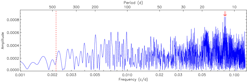
Burke et al. (2010) investigated a possible sinusoidal variation in the transit timing values with a period 118.3 orbital cycles, following a suggestion by B. Gary. They found that this more complex ephemeris provided a better fit to the data but by an amount which fell far short of statistical significance. To check this out we calculated a periodogram of the residuals of the best-fitting linear ephemeris with the period04 code (Lenz & Breger, 2004) covering the frequency range from 0.0 to the Nyquist frequency of 0.13 cycles per day (i.e. equivalent to twice the orbital period).
Fig. 6 shows the resulting frequency spectrum. The red dotted line indicates the possible period at 118.3 orbital cycles (466.3 d) mentioned by Burke et al. (2010): the periodogram shows no significant power at this period. The two strongest peaks are at much higher frequencies of 0.0807 and 0.0802 cycles per day, and both have a signal to noise ratio of 3.04. This is well below the value of 4.0 typically considered to be the level at which a frequency is significant (Breger et al., 1993, e.g.). We therefore conclude that there is no evidence for a periodic variation in the orbital ephemeris of XO-1.
6 The optical-infrared transmission spectrum of XO-1 b
We now study how the transit depth varies as a function of wavelength. This effect is caused by changes in the apparent radius of the planet, which in turn arise from variations in opacity and scattering processes in its extended atmosphere. Its transmission spectrum therefore potentially holds information about the abundances of atoms and molecules, and the temperature structure of the atmosphere.
Following the approach of Southworth et al. (2012), we modelled all available transit light curves of XO-1 in order to measure the planet radius (in the form of ) as a function of wavelength. It is important to fix the geometric parameters to representative values in order to maximise the consistency between different light curve fits and to avoid sources of uncertainty which are common to all light curves. The choice of these parameters is not simple because of conflicting results from published transmission spectroscopic studies of XO-1 b.
6.1 Consideration of published results


Tinetti et al. (2010) presented HST/NICMOS observations of a transit of XO-1 which yielded a transmission spectrum covering 1.2–1.8 m. They claimed the detection of H2O, CH4 and CO2 molecules in the planetary atmosphere. Burke et al. (2010) extended this analysis to the geometric parameters of the system, and included a second (or should that be first?) NICMOS observation of XO-1 obtained 12 days (three planetary orbits) prior to the observations utilised by Tinetti et al. (2010).
Gibson et al. (2011) presented a reanalysis of the NICMOS data used by Tinetti et al. (2010), with differences of approach concerning the use of decorrelation parameters to remove systematic errors in the data which arise from both HST and NICMOS. Gibson et al. (2011) obtained a more scattered and much more uncertain transmission spectrum, and concluded that the detection of molecules claimed by Tinetti et al. (2010) was not supported by the data. Gibson et al. (2011) concluded that NICMOS is not a suitable instrument for transmission spectroscopy as it displays unremovable systematics of similar size to the astrophysical signal being sought.
Crouzet et al. (2012) also presented a reanalysis of the NICMOS observations from Tinetti et al. (2010), but also included the second transit of XO-1 observed 12 days earlier. They performed a similar reduction of the data as Tinetti et al. (2010) and Gibson et al. (2011), but with some different choices of instrumental parameters against which the light curves were decorrelated. They found results which were much closer to those of Tinetti et al. (2010) than Gibson et al. (2011), but with important differences remaining at the level of the expected astrophysical signal in the transmission spectrum.
Deming et al. (2013) used the improved capabilities of HST/WFC3 to obtain a transmission spectrum of XO-1 b over the 1.12–1.65 m wavelength interval. This was used to claim a detection of water absorption in the planetary atmosphere, as well as to rule out spectral features at the level claimed by Tinetti et al. (2010). As the work by Deming et al. (2013) is based on a more modern analysis of data obtained using a better instrument than previous transmission spectroscopy, we have chosen to anchor our new results on the geometric parameters used in this work. They are, in turn, those found by Burke et al. (2010): (the inverse of the quoted quantity ) and .
6.2 Analysis method
For each light curve we calculated the best-fitting model with jktebop. We fixed at 0.0890, at 88.8∘ and the orbital period at a representative value. We fitted for , the time of mid-transit (to guard against possible orbital period variations) and the coefficients of the baseline polynomial (see Table 1). Uncertainties in were calculated using both Monte Carlo and residual-permutation simulations, and the larger errorbar for was retained in each case. We found that the uncertainties for the BUSCA -band light curve were relatively large, especially for the residual-permutation simulations: this is a result of the moderate differences between the two light curves and therefore is expected.
The phenomenon of LD deserves special consideration. In a recent work on GJ 1132 (Southworth et al., 2017), and in provisional analyses for the current work, we found that the transmission spectrum was significantly affected by way in which LD was treated. We therefore modelled the light curves with a range of ways of dealing with LD. The quadratic LD law is the most widely used in the literature, but recent theoretical studies (Espinoza & Jordán, 2016; Morello et al., 2017) have found that other laws, such as logarithmic and square-root (see Southworth, 2008, for the equations), are capable of matching theoretical LD predictions more precisely. Logarithmic should be better than square-root in the current case, particularly for the redder optical passbands under consideration (Van Hamme, 1993).
We therefore obtained solutions to the light curves using the quadratic, logarithmic and square-root LD laws, in each case with both coefficients fixed and with the linear coefficient fitted but the nonlinear coefficient fixed. For consistency we adopted theoretical LD coefficients obtained by Claret (2000); Claret (2004a) using the atlas9 atmosphere models (Kurucz, 1993), for all light curves, with the exception of the redshifted H filter for which we used LD coefficients from the Johnson filter tabulated by Van Hamme (1993).
For a comparison with the results above, and in order to capture the effect of differences in the LD coefficients used, we also fit each light curve using LD coefficients from Claret (2000); Claret (2004a) calculated using the phoenix model atmospheres. Fig. 7 shows the results for all alternatives investigated. It can be seen that the measured value of is not significantly affected by either the choice of LD law, whether or not one of the LD coefficients is fitted, or whether the LD coefficients come from the atlas9 or phoenix model atmospheres. We also notice – perhaps counterintuitively – that fixing both LD coefficients can yield larger errorbars despite the loss of one dimension from the area of parameter space in which the solution can be located. This occurs because fixing the LD coefficients can cause a poorer fit to the data, leading to larger errorbars from the residual-permutation algorithm.
From Fig. 7 we conclude that the treatment of LD does not have a significant effect on the results for individual light curves, and that it is safe to proceed with a representative set of measurements. One possible exception to this rule is the -band, for which the effect of LD treatment on the measured planet radius is significantly above the (very small) errorbars. Notwithstanding this, we chose as the representative set of values those measured using the quadratic LD law with the linear coefficient fitted at values from the atlas9 model atmospheres. Table 8 contains these values, and also for reference contains those from the quadratic LD law with both LD coefficients fixed. Table 8 also includes values for the central wavelength and full width at half maximum of the filters used to obtain our observations with BUSCA1010
10
https://www.caha.es/CAHA/Instruments/filterlist.html and the INT/WFC1111
11
http://catserver.ing.iac.es/filter/list.php?
instrument=WFC, and for published data obtained using the Palomar 50 in1212
12
http://www.astro.caltech.edu/palomar/observer/
60inchResources/p60filters.html, SofI1313
13
http://www.eso.org/sci/facilities/lasilla/
instruments/sofi/inst/Imaging.html and ISAAC1414
14
http://www.eso.org/sci/facilities/paranal/
decommissioned/isaac/doc/VLT-MAN-ESO-14100-0841_v90.pdf instruments.
6.3 Results
| Data | Filter | Central | Band full | ||||
|---|---|---|---|---|---|---|---|
| source | wavelength (nm) | width (nm) | (LD fixed | (LD fitted) | |||
| INT/WFC | redshifted H | 689 | 10 | 0.011983 | 0.000210 | 0.011911 | 0.000150 |
| BUSCA | SDSS | 366 | 38 | 0.011844 | 0.000129 | 0.011690 | 0.000129 |
| BUSCA | SDSS | 478 | 150 | 0.011483 | 0.000048 | 0.011450 | 0.000035 |
| BUSCA | SDSS | 663 | 105 | 0.011840 | 0.000074 | 0.011698 | 0.000123 |
| BUSCA | SDSS | 910 | 90 | 0.011906 | 0.000126 | 0.011837 | 0.000112 |
| CAHA 1.23 m | Cousins | 810 | 110 | 0.011804 | 0.000074 | 0.011741 | 0.000071 |
| Holman FLWO | SDSS | 0.011716 | 0.000075 | 0.011750 | 0.000069 | ||
| Holman Palomar | Cousins | 647 | 152 | 0.011297 | 0.000196 | 0.011231 | 0.000164 |
| Cáceres SofI | 1247 | 290 | 0.011725 | 0.000170 | 0.011719 | 0.000175 | |
| Cáceres ISAAC | + block | 1250 | 290 | 0.011907 | 0.000208 | 0.011822 | 0.000265 |
| Sada | 0.011170 | 0.000355 | 0.011880 | 0.000437 | |||
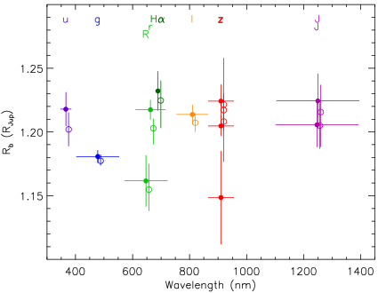
In Fig. 8 we show the transmission spectrum of XO-1 b determined from the light curves studied in this work, both new and previously published. Our preferred approach is to fit for the linear LD coefficient, and these results are shown as filled circles. The alternative approach of fixing both LD coefficients yields the results shown using open circles. Fig. 8 shows the values of obtained by multiplying the values in Table 8 by the semimajor axis (0.04914 AU) and a conversion factor (1 AU 2092.5).
It is immediately apparent from Fig. 8 that different light curves in the same or similar passbands show significant variations in . On closer inspection the two worst offenders are the Palomar -band data from Holman et al. (2006) and the -band light curve from Sada et al. (2012). Both have a high scatter and include no observations on one side of the transit, so it is not surprising that they give values which are very uncertain. This issue can be dealt with either by combining results from multiple light curves in the same or similar passbands or by ignoring the problematic results. In the current case, both options give a similar outcome.
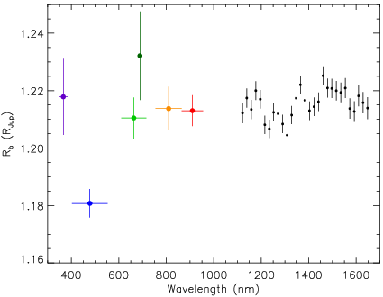
In Fig. 9 we show the transmission spectrum of XO-1 b after some consolidation of the results. The three -band values have been reduced into their weighted mean, as have the Palomar and BUSCA bands, in order to stop their large errorbars obfuscating such plots. We have not combined the redshifted H result with any other as the value of from this light curve has much greater wavelength resolution (resolving power ) than the and bands. We have furthermore ignored the -band results from now on because they add nothing to our analysis: they are consistent with and are completely overlapped by published transmission spectra, but are of lower precision and much lower wavelength resolution.
In Fig. 9 we have also plotted the HST/WFC3 transmission spectrum of XO-1 b obtained by Deming et al. (2013), after converting it from the values of (Deming et al., 2013, their table 3) to consistently with our values of . The treatment of LD by Deming et al. (2013) is relevant: they used the linear LD law with coefficients fixed to values interpolated from the - and -band coefficients tabulated by Claret & Bloemen (2011). They account for minor variations between different sources of theoretical LD coefficients, but do not allow for any imperfections in the description of real stars by current theoretical model atmospheres. They also neglect the spectral variation of LD coefficients over wavelength intervals smaller than those of the broad-band and filters. This approach is quite simplistic, but has less impact in the infrared than at visual wavelengths, because stellar LD is weaker in the infrared.
6.4 Interpretation

We used a forward transmission spectrum model to fit the optical and near infrared data of XO-1 b. For the pressure-temperature profile, we use the parameterisation of Madhusudhan & Seager (2009) which consists of six free parameters. We partitioned our model atmosphere into 100 layers spaced equally in log-pressure between bar and bar. For the atmospheric composition, we considered several chemical species with prevalent signatures in the the spectral range of the optical and near-infrared observations (Madhusudhan, 2012; Moses et al., 2013; Venot et al., 2015). These include Na, K, H2O, NH3, HCN, and CH4. The mixing ratio of each species was assumed to be uniform in the observable atmosphere and we assumed an atmosphere rich in H2 and He with a He/H2 ratio of 0.17. We considered line absorption from each molecular species and collision-induced opacity from H2-H2 and H2-He. The sources of opacity for the chemical species are described in Gandhi & Madhusudhan (2017); Gandhi & Madhusudhan (2018). In addition, we accounted for cloud effects due to small and large modal particle sizes. Large cloud particles were represented by a grey opacity throughout the whole spectrum and small cloud particles and/or hazes modified the H2 scattering Rayleigh slope in the optical.
The full set of observations were best fitted (Fig. 10) with a patchy cloud model having a terminator cloud and haze fraction of 0.54. The patchy cloud model is generally preferred to a clear-atmosphere model at the 1.3 confidence level. H2O is present at 3.05 confidence to fit the HST/WFC3 data, signifying water vapour is present with a certainty of 99.87%. Nitrogen chemistry (NH3 and HCN) is hinted at 1.5. The data do not provide evidence for the presence of either Na or K in the planetary atmosphere. Our model fits the optical transmission spectrum in the , /, and bands to within 0.5.
The best-fit model is unable to explain the measured planet radius in the band, which lies 8 below the model transmission spectrum and well below all other planet radius measurements. The reason for this discrepancy is not clear but is very difficult to explain theoretically, as none of our model transmission spectra exhibit a planet radius at any point in the optical which is below the radii in the infrared. It is also hard to understand observationally, as the two light curves in this passband are of high precision and very good mutual agreement, and such an effect has not been seen in this band in previous observations by our team1515 15 For example WASP-57 (Southworth et al., 2015), HAT-P-23 and WASP-48 (Ciceri et al., 2015), Qatar-2 (Mancini et al., 2014) and HAT-P-32 (Tregloan-Reed et al., 2018).. Temporal variability of the planet or stellar (Oshagh et al., 2014; Rackham et al., 2017, e.g.) atmosphere cannot be culpable because both -band light curves were obtained simultaneously with -band and either -band or -band observations.
We conclude that the transmission spectrum is best reproduced by a H2/He-rich planetary atmosphere containing H2O with low confidence levels of patchy clouds and nitrogen-bearing molecules (NH3 and HCN). An anomalously small planet radius in the -band is difficult to explain either observationally or theoretically and should be investigated by obtaining new observations in this wavelength region, preferably with a significantly higher resolution.
6.5 Discrepant transit depths
The referee expressed concern over the discrepant transit depth obtained from the -band light curves. It is clear that there is something affecting the -band data which is not accounted for in our data reduction and analysis procedures. These datasets were processed through the same data reduction and analysis programs as used by our group in many previous studies, which implies that the problem lies with the data themselves rather than with the reduction and analysis. Based on this, we rejected the -band data from the analysis of the transmission spectrum. This implicitly assumes that the problem is isolated to the -band alone; our results could be affected if the problem exists in other light curves or is an artefact of our data reduction pipeline.
We chose not to reject the -band data when determining the physical properties of the system, and have assessed the impact of this choice by rerunning the analysis without the -band data. We find that the final photometric results (Table 3) differ by 0.3 for and less than 0.1 for and . The physical properties of the system in Table 5 are unchanged except that increases by 0.2 and decreases by 0.3. The inclusion of the -band data therefore does not have a significant effect on the measured physical properties of the XO-1 system.
6.6 Impact of the optical data

One purpose of the current work was to see what improvement in our understanding of the properties of the atmosphere of XO-1 b could be obtained by adding optical transit data to the HST near-infrared transmission spectrum. We investigated this by modelling both the full transmission spectrum and the HST results only.
We find that the addition of the optical data to the near-infrared observations introduces an alternative water abundance estimate. Fig. 11 shows the retrieved water abundances for the case of our optical observations plus the HST data, and for the HST data alone. In the latter case the modal H2O abundance is approximately dex with a median and errorbars of . The slight tail of the posterior distribution arises from a weak degeneracy with HCN. The adjoined observations in the visible offer a complementary interpretation of XO-1 b’s atmosphere, adding a second mode to the H2O mixing ratio at dex and thus altering the median abundance by approximately dex.
The two interpretations of XO-1 b’s atmospheric H2O concentration emerge from two possible cloud condensate configurations. The water abundance mode at approximately dex that is introduced by the optical data suggests an atmosphere with condensate clouds composed of particle sizes 1 m whose cloud-top pressures are 0.01 to 0.1 mbar. The formation efficiency of condensate particles decreases with atmospheric height (Parmentier et al., 2013), and therefore clouds extending to low pressures of 0.01–0.1 mbar require vertical mixing processes such as convection which could advect material upward. On the other hand, the second mode constituting a high water abundance of approximately dex proposes cloud-top pressures greater than 1 mbar. Ultimately, elucidating the atmosphere of XO-1 b from these two distinct possibilities (low water abundance/high-extending clouds, and high water abundance/low-extending clouds) will have to await more precise observations in the optical.
7 Summary and discussion
XO-1 has been identified as a good candidate for the JWST Early Release Science program (Stevenson et al., 2016). A near-infrared transmission spectrum for XO-1 b has previously been obtained using HST/WFC3, resulting in the detection of water in the planetary atmosphere. We have obtained a total of ten high-precision transit light curves covering the full optical wavelength range (366 nm to 910 nm) in order to extend this transmission spectrum to optical wavelengths.
We use our data, alongside published transit light curves and spectroscopic quantities of the host star, to measure the physical properties of the system. Our results are in good agreement with, and more precise than, previous studies. We also assemble all available transit timing measurements and derive a high-precision orbital ephemeris useful for scheduling future observations. We find no evidence for periodic deviations from this ephemeris, contrary to previous suggestions. The non-detection of any quadratic deviation from the linear ephemeris allows us to constrain the tidal quality factor for the host star to be .
We fitted the transit light curves using the same system geometry as for the HST/WFC3 observations, in order to measure the radius of the planet as a function of wavelength. This optical-infrared transmission spectrum is well fitted by a model spectrum for a planet with a H2/He-rich atmosphere and patchy cloud. H2O is detected to 3.05 while suggestions of patchy clouds (1.3) and nitrogen chemistry (1.5) are weak given the present observations. We find that adding the optical to the near-infrared data leads to less precise constraints on the planetary atmosphere. This indicates that optical observations of a higher precision and spectral resolution would be needed to improve our understanding of the atmosphere of XO-1 b, and also that there is some tension between the best-fitting atmospheric properties in the optical and in the near-infrared. The planet radius we measure in the -band is anomalously low, a finding difficult to explain either observationally or theoretically. We advocate further observations in this wavelength region, with a higher spectral resolution.
Throughout this work we have paid careful attention to the treatment of LD when fitting transit light curves. When measuring the physical properties of the system we used four different LD laws and two different approaches to fitting the coefficients of these. We find that the range of solutions produced by these different fits is very small when fitting high-quality data, so the treatment of LD is thankfully not a significant hindrance to measuring the system properties. From a similarly detailed investigation concerning the transmission spectrum, we find that the choice of LD law, and whether or not to fit for one of the coefficients, is unimportant, giving rise to a scatter in the planet radius measurements which is small compared to the variation between light curves. The only exception to this rule is for the -band, where the very small uncertainties in the planet radius do not fully cover the scatter between solutions with a different treatment of LD. Whilst the situation for XO-1 is encouraging, we urge that similar analysis should be performed as standard procedure when obtaining transmission spectra. This is particularly true for planets transiting low-mass stars, whose LD may not be well captured by parametric laws and for which LD coefficients are more difficult to derive theoretically.
We confirm that XO-1 is an excellent target for future observations with JWST. Its physical properties are well-understood, the planet’s transmission spectrum has features comparatively easy to measure using existing instrumentation, its solar-type host star shows no sign of chromospheric activity, and our new orbital ephemeris is precise enough to predict transits to within 5 s up to the year 2266.
Acknowledgements
We thank the referee for comments which improved the paper and encouraged us to test the reliability of our results. The reduced light curves presented in this work will be made available at the CDS (http://vizier.u-strasbg.fr/) and at http://www.astro.keele.ac.uk/jkt/. JS acknowledges financial support from the Leverhulme Trust in the form of a Philip Leverhulme Prize. AP is grateful for research funding from the Gates Cambridge Trust. LM acknowledges support from the Italian Minister of Instruction, University and Research (MIUR) through FFABR 2017 fund, and from the Department of Physics of the University of Rome Tor Vergata, through Mission Sustainability 2016 funds. The following internet-based resources were used in research for this paper: the ESO Digitized Sky Survey; the NASA Astrophysics Data System; the SIMBAD database and VizieR catalogue access tool operated at CDS, Strasbourg, France; and the ariv scientific paper preprint service operated by Cornell University. Based on observations collected at the Centro Astronómico Hispano Alemán (CAHA) at Calar Alto, Spain, operated jointly by the Max-Planck Institut für Astronomie and the Instituto de Astrofísica de Andalucía (CSIC), and on observations made with the Isaac Newton Telescope operated on the island of La Palma by the Isaac Newton Group in the Spanish Observatorio del Roque de los Muchachos of the Instituto de Astrofísica de Canarias
References
- Akaike (1974) Akaike, H., 1974, IEEE Transactions on Automatic Control, 19, 716
- Ammler-von Eiff et al. (2009) Ammler-von Eiff, M., Santos, N. C., Sousa, S. G., Fernandes, J., Guillot, T., Israelian, G., Mayor, M., Melo, C., 2009, A&A, 507, 523
- Anderson et al. (2012) Anderson, D. R., et al., 2012, MNRAS, 422, 1988
- Beichman et al. (2014) Beichman, C., et al., 2014, PASP, 126, 1134
- Birkby et al. (2014) Birkby, J. L., et al., 2014, MNRAS, 440, 1470
- Bonomo et al. (2017) Bonomo, A. S., et al., 2017, A&A, 602, A107
- Breger et al. (1993) Breger, M., et al., 1993, A&A, 271, 482
- Brewer et al. (2016) Brewer, J. M., Fischer, D. A., Valenti, J. A., Piskunov, N., 2016, ApJS, 225, 32
- Burke et al. (2010) Burke, C. J., et al., 2010, ApJ, 719, 1796
- Cáceres et al. (2009) Cáceres, C., Ivanov, V. D., Minniti, D., Naef, D., Melo, C., Mason, E., Selman, F., Pietrzynski, G., 2009, A&A, 507, 481
- Carter et al. (2008) Carter, J. A., Yee, J. C., Eastman, J., Gaudi, B. S., Winn, J. N., 2008, ApJ, 689, 499
- Charbonneau et al. (2002) Charbonneau, D., Brown, T. M., Noyes, R. W., Gilliland, R. L., 2002, ApJ, 568, 377
- Ciceri et al. (2015) Ciceri, S., et al., 2015, A&A, 577, A54
- Claret (2000) Claret, A., 2000, A&A, 363, 1081
- Claret (2004a) Claret, A., 2004a, A&A, 428, 1001
- Claret (2004b) Claret, A., 2004b, A&A, 424, 919
- Claret & Bloemen (2011) Claret, A., Bloemen, S., 2011, A&A, 529, A75
- Claret & Hauschildt (2003) Claret, A., Hauschildt, P. H., 2003, A&A, 412, 241
- Crouzet et al. (2012) Crouzet, N., McCullough, P. R., Burke, C., Long, D., 2012, ApJ, 761, 7
- Demarque et al. (2004) Demarque, P., Woo, J.-H., Kim, Y.-C., Yi, S. K., 2004, ApJS, 155, 667
- Deming et al. (2013) Deming, D., et al., 2013, ApJ, 774, 95
- Dotter et al. (2008) Dotter, A., Chaboyer, B., Jevremović, D., Kostov, V., Baron, E., Ferguson, J. W., 2008, ApJS, 178, 89
- Eastman et al. (2010) Eastman, J., Siverd, R., Gaudi, B. S., 2010, PASP, 122, 935
- Espinoza & Jordán (2016) Espinoza, N., Jordán, A., 2016, MNRAS, 457, 3573
- Evans et al. (2016) Evans, D. F., Southworth, J., Smalley, B., 2016, ApJ, 833, L19
- Fischer et al. (2016) Fischer, P. D., et al., 2016, ApJ, 827, 19
- Fukugita et al. (1996) Fukugita, M., Ichikawa, T., Gunn, J. E., Doi, M., Shimasaku, K., Schneider, D. P., 1996, AJ, 111, 1748
- Gandhi & Madhusudhan (2017) Gandhi, S., Madhusudhan, N., 2017, MNRAS, 472, 2334
- Gandhi & Madhusudhan (2018) Gandhi, S., Madhusudhan, N., 2018, MNRAS, 474, 271
- Gibson et al. (2011) Gibson, N. P., Pont, F., Aigrain, S., 2011, MNRAS, 411, 2199
- Greene et al. (2016) Greene, T. P., Line, M. R., Montero, C., Fortney, J. J., Lustig-Yaeger, J., Luther, K., 2016, ApJ, 817, 17
- Holman et al. (2006) Holman, M. J., et al., 2006, ApJ, 652, 1715
- Jackson et al. (2008) Jackson, B., Greenberg, R., Barnes, R., 2008, ApJ, 678, 1396
- Jackson et al. (2009) Jackson, B., Barnes, R., Greenberg, R., 2009, ApJ, 698, 1357
- Johnson (1964) Johnson, H. L., 1964, Boletin de los Observatorios Tonantzintla y Tacubaya, 3, 305
- Knutson et al. (2010) Knutson, H. A., Howard, A. W., Isaacson, H., 2010, ApJ, 720, 1569
- Kurucz (1993) Kurucz, R., 1993, ATLAS9 stellar atmosphere programs and 2 km/s grid. Kurucz CD-ROM No. 13
- Lenz & Breger (2004) Lenz, P., Breger, M., 2004, in J. Zverko, J. Žižnovsky, S. J. Adelman, & W. W. Weiss, ed., The A-Star Puzzle, Cambridge University Press, Cambridge, UK., vol. 224 of IAU Symposium, p. 786
- Levrard et al. (2009) Levrard, B., Winisdoerffer, C., Chabrier, G., 2009, ApJ, 692, L9
- Love (1911) Love, A. E. H., 1911, Some Problems of Geodynamics, Cambridge University Press, Cambridge, 1911
- Machalek et al. (2008) Machalek, P., McCullough, P. R., Burke, C. J., Valenti, J. A., Burrows, A., Hora, J. L., 2008, ApJ, 684, 1427
- Madhusudhan (2012) Madhusudhan, N., 2012, ApJ, 758, 36
- Madhusudhan & Seager (2009) Madhusudhan, N., Seager, S., 2009, ApJ, 707, 24
- Madhusudhan & Winn (2009) Madhusudhan, N., Winn, J. N., 2009, ApJ, 693, 784
- Madhusudhan et al. (2014) Madhusudhan, N., Amin, M. A., Kennedy, G. M., 2014, ApJ, 794, L12
- Mamajek & Hillenbrand (2008) Mamajek, E. E., Hillenbrand, L. A., 2008, ApJ, 687, 1264
- Mancini et al. (2014) Mancini, L., et al., 2014, MNRAS, 443, 2391
- Markquardt (1963) Markquardt, D. W., 1963, J. Soc. Ind. Appl. Math., 11, 431
- Maxted et al. (2015) Maxted, P. F. L., Serenelli, A. M., Southworth, J., 2015, A&A, 577, A90
- McCullough et al. (2006) McCullough, P. R., et al., 2006, ApJ, 648, 1228
- Mordasini et al. (2016) Mordasini, C., van Boekel, R., Mollière, P., Henning, T., Benneke, B., 2016, ApJ, 832, 41
- Morello et al. (2017) Morello, G., Tsiaras, A., Howarth, I. D., Homeier, D., 2017, AJ, 154, 111
- Mortier et al. (2013) Mortier, A., Santos, N. C., Sousa, S. G., Fernandes, J. M., Adibekyan, V. Z., Delgado Mena, E., Montalto, M., Israelian, G., 2013, A&A, 558, A106
- Moses et al. (2013) Moses, J. I., Madhusudhan, N., Visscher, C., Freedman, R. S., 2013, ApJ, 763, 25
- Nikolov et al. (2016) Nikolov, N., Sing, D. K., Gibson, N. P., Fortney, J. J., Evans, T. M., Barstow, J. K., Kataria, T., Wilson, P. A., 2016, ApJ, 832, 191
- Ogilvie (2014) Ogilvie, G. I., 2014, ARA&A, 52, 171
- Ogilvie & Lin (2007) Ogilvie, G. I., Lin, D. N. C., 2007, ApJ, 661, 1180
- Oshagh et al. (2014) Oshagh, M., Santos, N. C., Ehrenreich, D., Haghighipour, N., Figueira, P., Santerne, A., Montalto, M., 2014, A&A, 568, A99
- Pál (2008) Pál, A., 2008, MNRAS, 390, 281
- Parmentier et al. (2013) Parmentier, V., Showman, A. P., Lian, Y., 2013, A&A, 558, A91
- Penev & Sasselov (2011) Penev, K., Sasselov, D., 2011, ApJ, 731, 67
- Penev et al. (2012) Penev, K., Jackson, B., Spada, F., Thom, N., 2012, ApJ, 751, 96
- Pietrinferni et al. (2004) Pietrinferni, A., Cassisi, S., Salaris, M., Castelli, F., 2004, ApJ, 612, 168
- Poddaný et al. (2010) Poddaný, S., Brát, L., Pejcha, O., 2010, New Astronomy, 15, 297
- Pollacco et al. (2006) Pollacco, D. L., et al., 2006, PASP, 118, 1407
- Pont et al. (2011) Pont, F., Husnoo, N., Mazeh, T., Fabrycky, D., 2011, MNRAS, 414, 1278
- Pont et al. (2013) Pont, F., Sing, D. K., Gibson, N. P., Aigrain, S., Henry, G., Husnoo, N., 2013, MNRAS, 432, 2917
- Press et al. (1992) Press, W. H., Teukolsky, S. A., Vetterling, W. T., Flannery, B. P., 1992, Numerical Recipes in FORTRAN 77. The art of scientific computing, Cambridge: University Press, 2nd ed.
- Rackham et al. (2017) Rackham, B., et al., 2017, ApJ, 834, 151
- Raetz et al. (2009) Raetz, S., et al., 2009, AN, 330, 475
- Sada et al. (2012) Sada, P. V., et al., 2012, PASP, 124, 212
- Schwarz (1978) Schwarz, G., 1978, Annals of Statistics, 5, 461
- Seager & Mallén-Ornelas (2003) Seager, S., Mallén-Ornelas, G., 2003, ApJ, 585, 1038
- Sing et al. (2016) Sing, D. K., et al., 2016, Nature, 529, 59
- Skrutskie et al. (2006) Skrutskie, M. F., et al., 2006, AJ, 131, 1163
- Southworth (2008) Southworth, J., 2008, MNRAS, 386, 1644
- Southworth (2009) Southworth, J., 2009, MNRAS, 394, 272
- Southworth (2010) Southworth, J., 2010, MNRAS, 408, 1689
- Southworth (2011) Southworth, J., 2011, MNRAS, 417, 2166
- Southworth (2012) Southworth, J., 2012, MNRAS, 426, 1291
- Southworth (2013) Southworth, J., 2013, A&A, 557, A119
- Southworth & Evans (2016) Southworth, J., Evans, D. F., 2016, MNRAS, 463, 37
- Southworth et al. (2012) Southworth, J., Mancini, L., Maxted, P. F. L., Bruni, I., Tregloan-Reed, J., Barbieri, M., Ruocco, N., Wheatley, P. J., 2012, MNRAS, 422, 3099
- Southworth et al. (2017) Southworth, J., Mancini, L., Madhusudhan, N., Mollière, P., Ciceri, S., Henning, T., 2017, AJ, 153, 191
- Southworth et al. (2009) Southworth, J., et al., 2009, MNRAS, 396, 1023
- Southworth et al. (2014) Southworth, J., et al., 2014, MNRAS, 444, 776
- Southworth et al. (2015) Southworth, J., et al., 2015, MNRAS, 454, 3094
- Southworth et al. (2016) Southworth, J., et al., 2016, MNRAS, 457, 4205
- Stetson (1987) Stetson, P. B., 1987, PASP, 99, 191
- Stevenson et al. (2016) Stevenson, K. B., et al., 2016, PASP, 128, 094401
- Teske et al. (2014) Teske, J. K., Cunha, K., Smith, V. V., Schuler, S. C., Griffith, C. A., 2014, ApJ, 788, 39
- Tinetti et al. (2010) Tinetti, G., Deroo, P., Swain, M. R., Griffith, C. A., Vasisht, G., Brown, L. R., Burke, C., McCullough, P., 2010, ApJ, 712, L139
- Torres et al. (2008) Torres, G., Winn, J. N., Holman, M. J., 2008, ApJ, 677, 1324
- Torres et al. (2012) Torres, G., Fischer, D. A., Sozzetti, A., Buchhave, L. A., Winn, J. N., Holman, M. J., Carter, J. A., 2012, ApJ, 757, 161
- Tregloan-Reed et al. (2018) Tregloan-Reed, J., et al., 2018, MNRAS, 474, 5485
- Tsiaras et al. (2018) Tsiaras, A., et al., 2018, AJ, 155, 156
- Van Hamme (1993) Van Hamme, W., 1993, AJ, 106, 2096
- VandenBerg et al. (2006) VandenBerg, D. A., Bergbusch, P. A., Dowler, P. D., 2006, ApJS, 162, 375
- Vaňko et al. (2009) Vaňko, M., et al., 2009, in Pont, F., Sasselov, D., Holman, M. J., eds., Transiting Planets, vol. 253 of IAU Symposium, p. 440
- Venot et al. (2015) Venot, O., Hébrard, E., Agúndez, M., Decin, L., Bounaceur, R., 2015, A&A, 577, A33
- Wilkins et al. (2017) Wilkins, A. N., Delrez, L., Barker, A. J., Deming, D., Hamilton, D., Gillon, M., Jehin, E., 2017, ApJ, 836, L24
- Wilson et al. (2006) Wilson, D. M., et al., 2006, PASP, 118, 1245
- Wöllert et al. (2015) Wöllert, M., Brandner, W., Bergfors, C., Henning, T., 2015, A&A, 575, A23