Effect of van-Hove singularities in single-walled carbon nanotube leads on transport through double quantum dot system

We now study, the effect of swapping energy levels of the dots. In Fig. 4, we plot conductance as a function of chemical potential $\mu$ in the armchair $(5,5)$ CNT leads for two different values of the interdot tunneling matrix-element $t=0.07U,0.1U$. The energy levels of the dots, in Figs. 4(a) and 4(b) are respectively kept as $\varepsilon_{1}=0.56U$, $\varepsilon_{2}=0.589U$ and $\varepsilon_{1}=0.589U$, $\varepsilon_{2}=0.56U$ with interdot Coulomb interaction $g=0.08U$. In either case, $\left|\varepsilon_{1}-\varepsilon_{2}\right|=0.029U$ and the energy level of one of the two dots is aligned with the first vHs about the Fermi level in the DOS of the armchair $(5,5)$ CNT leads at $0.589$. The ground states of the isolated DQD system with $U_{1}=U_{2}=U$ corresponding to one, three and four electrons are respectively given as $\lambda^{0}_{1e}=\frac{1}{2}\left[\varepsilon_{1}+\varepsilon_{2}-\sqrt{(\varepsilon_{1}-\varepsilon_{2})^{2}+4t^{2}}\right]$, $\lambda^{0}_{3e}=\frac{1}{2}\left[3\left(\varepsilon_{1}+\varepsilon_{2}\right)+4g+2U-\sqrt{(\varepsilon_{1}-\varepsilon_{2})^{2}+4t^{2}}\right]$, and $\lambda^{0}_{4e}=2(\varepsilon_{1}+\varepsilon_{2})+4g+2U$, whereas for two electrons $\lambda^{0}_{2e}$ is obtained numerically. At zero temperature, the four peaks would appear at the positions $\lambda^{0}_{1e}=0.5030$, $\lambda^{0}_{2e}-\lambda^{0}_{1e}=0.7051$, $\lambda^{0}_{3e}-\lambda^{0}_{2e}=1.6039$ and $\lambda^{0}_{4e}-\lambda^{0}_{3e}=1.8060$, respectively. But the positions of peaks in Fig. 4 are slightly shifted due to several factors such as the temperature, ondot and interdot interactions also coupling to the leads. The actual positions of respective four peaks for $t=0.07U$, as read from Figs. 4(a) or 4(b) are at $0.50$, $0.64$, $1.70$ and $2.08$. The splitting between any two corresponding peaks in Figs. 4(a) and 4(b) remains the same, but the heights of the peaks are different. It is seen that with $\varepsilon_{1}<\varepsilon_{2}$ in Fig. 4(a), there is alternate suppression in the peak heights, i.e. the heights of the second and fourth peaks are less as compared to the first and third peaks, respectively. Whereas for $\varepsilon_{1}>\varepsilon_{2}$ in Fig. 4(b), the heights of the first and third peaks are less as compared to the second and fourth peaks, respectively. In either case, the first and second peaks exhibit significant change in their heights as compared to the third and the fourth peak heights. With this observation, one may attribute the alternate suppression of peak heights to the effect of aligning one of the dot levels with the position of the vHs in the DOS of CNT leads. This we further investigate in the following.

To examine it further, in Fig. 5, we plot conductance as a function of chemical potential $\mu$ in the armchair $(5,5)$ CNT leads for same values of parameters as in Fig. 4, except that the dot levels in Fig. 5(a), are kept at values $\varepsilon_{1}=0.971U$, $\varepsilon_{2}=1.0U$ and in Fig. 5(b), at values $\varepsilon_{1}=1.0U$, $\varepsilon_{2}=0.971U$. The energy level of one of the two dots, in either case is aligned with the second vHs position; away from the Fermi level in the DOS of the armchair $(5,5)$ CNT at $1.0$. The dot levels are kept separated by the same value $\left|\varepsilon_{1}-\varepsilon_{2}\right|=0.029$ as in Fig. 4. It is observed from Figs. 4 and 5 that the conductance profiles in the two situations resemble, qualitatively. The difference lies only in the heights of peaks which are less in Fig. 5 compared to the ones in Fig. 4. This is due to the effect of variation in DOS of CNT leads.

In Fig. 6, we plot conductance as a function of chemical potential $\mu$ in the armchair $(5,5)$ CNT leads for two different values of the interdot tunneling matrix-element $t=0.07U,0.1U$. The dot levels in Fig. 6(a), are fixed to align with the first vHs position present near the Fermi level in the DOS of the armchair $(5,5)$ CNT at $0.589$ i.e. $\varepsilon_{1}=\varepsilon_{2}=0.589U$ and in Fig. 6(b), at same values closed to the Fermi level in the leads $\varepsilon_{1}=\varepsilon_{2}=0.10U$. A rough approximation of the positions of peaks, at zero temperature, can be obtained by the ground states of the isolated DQD system. The positions of all four peaks in this case can be obtained with $\varepsilon_{1}=\varepsilon_{2}=\varepsilon$ and $U_{1}=U_{2}=U$ from the results given above. The positions of the first, second, third and fourth peaks are given as $E_{0}^{1}=\varepsilon-t$, $E_{0}^{2}=\varepsilon+t+\frac{1}{2}\left(g+U-\sqrt{(U-g)^{2}+16t^{2}}\right)$, $E_{0}^{3}=(\varepsilon-t)+\frac{1}{2}(3g+U)+\frac{1}{2}\sqrt{(U-g)^{2}+4t^{2}}$ and $E_{0}^{4}=\varepsilon+t+2g+U$, respectively [38]. Using peak positions; peak separations $E_{0}^{i}-E_{0}^{j}$ between the peaks can also be obtained [56]. The corresponding positions of the peaks obtained using above expressions for $t=0.07$, in Fig. 6(a), are given as $0.5190$, $0.7182$, $1.6198$ and $1.8190$ whereas in Fig. 6(b), at $0.03$, $0.2292$, $1.1308$ and $1.33$. However, the actual positions are slightly different. It is observed that the heights of the peaks gradually fall and their widths broaden from the first to fourth peak. This is due to the electron-electron interaction which modifies each time an electron is added when $N-$electron chemical potential of isolated DQD system reached. The first peak corresponds to non-interacting case and is sharpest and tallest. This picture modifies when there are two electrons in the DQD system. Now, the two electrons can interact in two ways, they can stay on the same dot by costing an additional energy equal to the ondot Coulomb interaction $U$ or on different dot by costing an additional energy equal to the interdot Coulomb interaction $g$. Further, the three electron situation on DQD would necessarily cost an additional energy $U$ and also $g$ as one of the two dots must be doubly occupied. The four electron situation has only possible configuration that each dot is doubly occupied, necessitating an energy $U$ and $g$ to be further incorporated. The gradual peak broadening and falling from first to fourth peak is therefore caused by the electron-electron correlation at a fixed temperature.
It is observed that the heights of the second and third peaks in Fig. 6(a) are shorter as compared to the heights of the corresponding peaks in Fig. 6(b) whereas, the first and fourth peaks are nearly of the same heights. The DOS of the CNT leads slightly differs about the positions of the first and fourth peaks in two situations, but significantly differs about the second and third peaks positions.
The conductance profiles when energy levels of both the dots are kept at values $\varepsilon_{1}=\varepsilon_{2}=0.951U$ and $\varepsilon_{1}=\varepsilon_{2}=1.0U$ are found similar to those in Fig. 6(a). The DOS of CNT has vHs at these values as given in Table 1. The conductance profiles when energy levels of both the dots are kept at values $\varepsilon_{1}=\varepsilon_{2}=0.953U$ and $\varepsilon_{1}=\varepsilon_{2}=0.952U$ were observed to be almost identical as DOS of CNT vary very slightly at the positions of conductance peaks in two cases. These values lie close the vHs at $0.951$ in DOS of CNT; the conductance profiles in two cases are qualitatively similar to the above cases for $\varepsilon_{1}=\varepsilon_{2}$.

To investigate the effect of large separation between the energy levels of the dots, in Fig. 7, we plot conductance and the corresponding occupancies $<n_{i}>$ of the dots as a function of chemical potential $\mu$ in the armchair $(5,5)$ CNT leads at a fixed value of the interdot tunneling matrix-element $t=0.1U$ with $g=0.08U$ and $k_{B}T=0.02U$. The dot levels in Fig. 7(a), are kept at values $\varepsilon_{1}=0.59U$, $\varepsilon_{2}=0.4U$ and in Fig. 7(b), at $\varepsilon_{1}=0.4$, $\varepsilon_{2}=0.59U$. The dot levels are far separated by value $\left|\varepsilon_{1}-\varepsilon_{2}\right|=0.19U$. One of the two dots in either case is aligned with the first vHs position away from the Fermi level; present in the DOS of armchair $(5,5)$ CNT leads at $0.589$. It is observed that the alternate conductance peaks are suppressed similar to those seen in Figs. 4 and 5, but the differences between the heights of the suppressed and unsuppressed peaks are relatively large. The corresponding occupancies in Figs. 7(a) and 7(b), show plateau structures investigated as a function of chemical potential. The structure originates due the quantization of charge. The occupancies show that the peaks in the conductance profiles in Figs. 7(a) and 7(b), correspond to the jumps in the occupancies of dot-1 $\left<n_{1}\right>$. The sharp jump signifies narrow peak where the tapered as broad peak. In Fig. 7(a), corresponding to the first peak, the occupancy of the dot-1 is less than that of dot-2 i.e. $\left<n_{1}\right><\left<n_{2}\right>$, due to the fact that the energy level of dot-2 is fixed below that of the dot-1 i.e. $\varepsilon_{2}<\varepsilon_{1}$. There are only two pathways possible for electron transport in the system viz. $Source\rightarrow Dot-1\rightarrow Drain$ ($SD_{1}D$) and $Source\rightarrow Dot-1\rightarrow Dot-2\rightarrow Dot-1\rightarrow Drain$ ($SD_{1}D_{2}D_{1}D$). However, the conductance results due to the transport through the quantum mechanical superposition of these two paths [57, 11]. In one-electron situation with $\varepsilon_{2}<\varepsilon_{1}$, the path $SD_{1}D_{2}D_{1}D$ is more probable. In the two-electron situation, the second electron occupies dot-1 in order to avoid extra energy due to ondot Coulomb interaction $U$ therefore, the corresponding occupancy of dot-1 is more than that dot-2 i.e. $\left<n_{1}\right>>\left<n_{2}\right>$. In this situation, the path $SD_{1}D$ is more probable and there is a sharper jump in the occupation number of dot-1 $\left<n_{1}\right>$ leading to a narrow peak with long height. The third electron would prefer to occupy the dot-2, since $U$ (not $g$) will make a difference in the energy as $(2\varepsilon_{2}+U)<(2\varepsilon_{1}+U)$. The occupancy of dot-2 is therefore, more than that of dot-1 $\left<n_{2}\right>>\left<n_{1}\right>$, the path $SD_{1}D_{2}D_{1}D$ is more probable. There is a tapered jump in the occupation number of dot-1 $\left<n_{1}\right>$ due to electron-electron correlation leading to broad and short peak. Now, the fourth electron has only one possibility to occupy the first dot and to take the path $SD_{1}D$. The occupancy of dot-1, which is more than that of the dot-2 $\left<n_{1}\right>>\left<n_{2}\right>$, has a tapered jump due to correlation, lead to a peak further broader in the width. The peaks present in the conductance profile in Fig. 7(b), for $\varepsilon_{1}<\varepsilon_{2}$ has similar behavior to that in Fig. 7(a). In Fig. 7, one of the two dots in either case is aligned with the vHs position, but suppression in the heights of peaks are not due to vHs position rather due to large dot level separations.

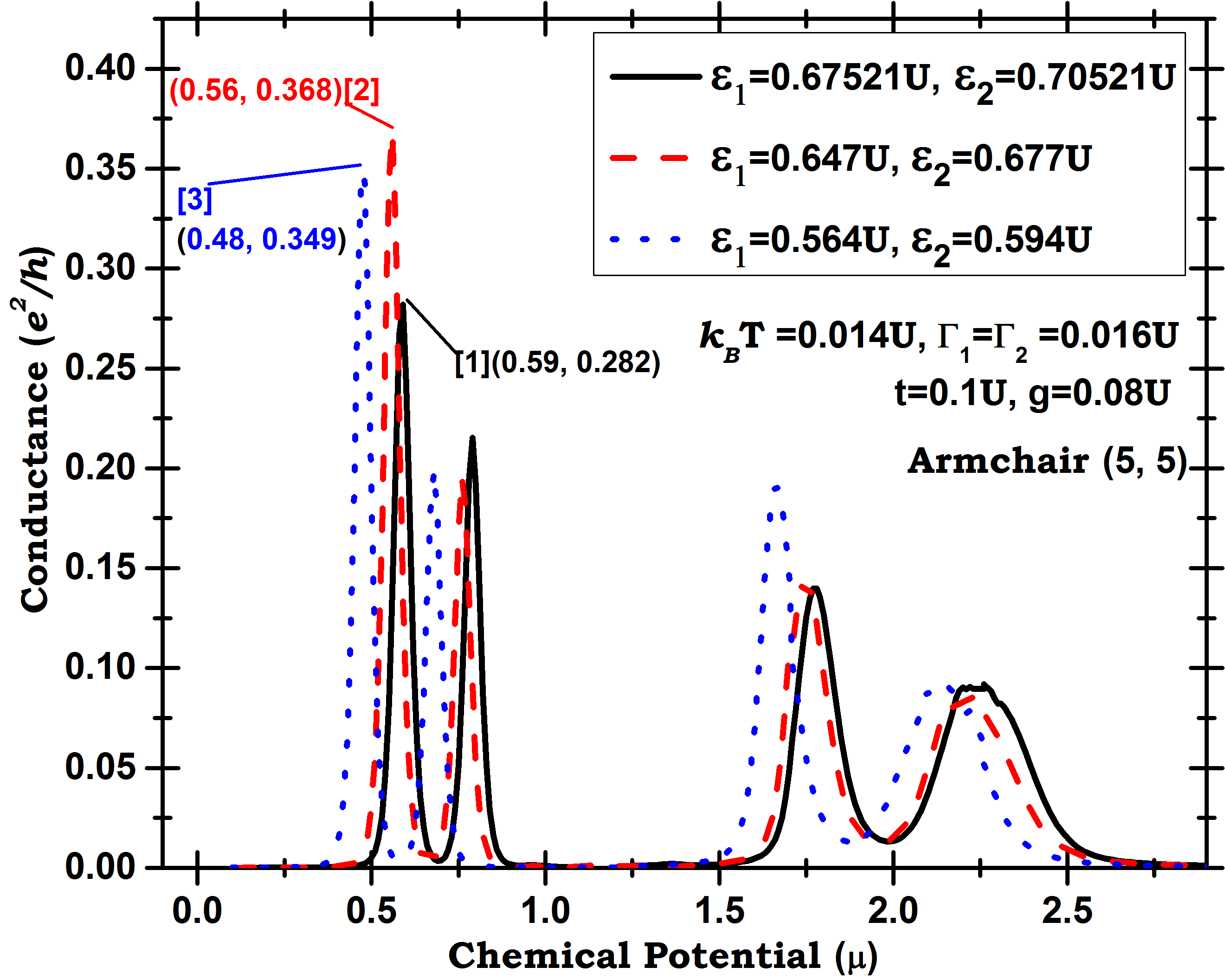
The study, so far has not revealed any distinctive attribute of the vHs. Now, we investigate the effect of one of the vHs present in the DOS of the armchair $(5,5)$ CNT leads. In Fig. 8, we plot, at a fixed value of the interdot tunneling matrix-element $t=0.1U$ with $g=0.08U$, the conductance as a function of chemical potential $\mu$ in the armchair $(5,5)$ CNT leads for three different set of values of the energy levels of two dots, in Fig. 8(a), for $\varepsilon_{1}=0.70521U$, $\varepsilon_{2}=0.67521U$; $\varepsilon_{1}=0.677U$, $\varepsilon_{2}=0.647U$ and $\varepsilon_{1}=0.594U$, $\varepsilon_{2}=0.564U$. Where in Fig. 8(b), for $\varepsilon_{1}=0.67521U$, $\varepsilon_{2}=0.70521U$; $\varepsilon_{1}=0.647U$, $\varepsilon_{2}=0.677U$ and $\varepsilon_{1}=0.564U$, $\varepsilon_{2}=0.594U$. The couplings, are taken even smaller $\Gamma_{1}=\Gamma_{2}=0.016U$, so that the many-body eigenstates of the DQD system are less affected. The temperature is kept as the smallest parameter $k_{B}T=0.014U<\Gamma_{1}(\Gamma_{2})$.

For a situation when two-electron chemical potential aligns with one of the vHs position, we plot in Fig. 9, the conductance for three different set of values of the energy levels $\left(\varepsilon_{1},\varepsilon_{2}\right)$ of QDs. The parameters are taken as $\varepsilon_{1}>\varepsilon_{2}$ such that the difference $\left|\varepsilon_{1}-\varepsilon_{2}\right|=0.03U$ and other parameters are the same as in Fig. 8. The set of values $\varepsilon_{1}=0.917U$, $\varepsilon_{2}=0.887U$ corresponding to solid curve are adjusted such that the two electron chemical potential of the isolated DQD system coincides with vHs present in DOS of armchair $(5,5)$ CNT at 1.0. For solid curve the positions of all four conductance peaks obtained using the eigenvalues of the isolated DQDs are respectively given as $0.801$, $1.042$, $1.922$ and $2.163$. From the results given in Figs. 4(b), 5(b), 7(a) and 8(a), we find that when $\varepsilon_{1}>\varepsilon_{2}$ the height of the second conductance peak is generally higher than that of the first peak. But, as can be noted that the height of the second conductance peak corresponding to the solid curve is less than that of the first peak whereas the heights of the second conductance peaks are higher than that of their corresponding first peaks for dashed and dotted curves. This observation is similar to the one observed in Fig. 8.

In order to further investigate the observations in Figs. 8 and 9, we plot in Fig. 10(b), the modified DOS of the armchair $(5,5)$ CNT. To clarify whether the effect of vHs manifests itself as fall in the height of the conductance peak or this is some numerical artifact. The DOS is modified in such a way that the vHs at $0.589$ is absent but the positions of the other vHs remain unchanged and the area under the curve is also unchanged. In Fig. 10(a), we plot, the conductance as a function of the chemical potential $\mu$ for the same values of parameters as in Fig. 8(a). The conductance profiles comes out to be different because of the modified DOS of the leads. The height of the first peak for solid curve corresponding to the set of values $\varepsilon_{1}=0.70521U$, $\varepsilon_{2}=0.67521U$ does not fall shorter as there is no vHs present to coincide at $0.589$ as in Fig. 8(a). Therefore, the conductance peaks can significantly fall in heights when their positions are aligned with the vHs in the CNT leads.

References

- [1] D. K. Ferry, S. M. Goodnick and J. Bird Transport in Nanostructures (Cambridge University Press, 2009).
- [2] S. Datta, Quantum Transport: Atom to Transistor (Cambridge University Press, 2005).
- [3] J. P. Bird, Electron Transport in Quantum Dots (Kluwer Academic Publishers, 2003).
- [4] I. L. Aleiner, P. W. Brouwer and L. I. Glazman, Phys. Rep. 358, 309 (2002).
- [5] Y. Alhassid, Rev. Mod. Phys. 72, 895 (2000).
- [6] K. Kang, S. Y. Cho, J. J. Kim and S. C. Shin, Phys. Rev. B 63, 113304 (2001).
- [7] M. E. Torio, K. Hallberg, A. H. Ceccatto and C. R. Proetto, Phys. Rev. B 65, 085302 (2002).
- [8] R. Franco, M. S. Figueira and E. V. Anda, Phys. Rev. B 67, 155301 (2003).
- [9] M. A. Kastner, Rev. Mod. Phys. 64, 849 (1992).
- [10] H. Grabert and M. H. Devoret, Single Charge Tunneling: Coulomb Blockade Phenomena in Nanostructures (Plenum press, New York, 1992).
- [11] S. Chand, R. K. Moudgil and P. K. Ahluwalia, Physica B 405 239-246 (2010).
- [12] J. Fransson and O. Eriksson, Phys. Rev. B 70 085301 (2004).
- [13] M. L. Ladron de Guevara, F. Claro and P. A. Orellana,Phys. Rev. B 67 195335 (2003).
- [14] J. J. Palacios and P. Hawrylak, Phys. Rev. B 51, 1769 (1995).
- [15] D. Loss and D. P. DiVincenzo, Phys. Rev. A 57, 120 (1998).
- [16] D. Loss and E. V. Sukhorukov, Phys. Rev. Lett. 84, 1035 (2000).
- [17] Hu and S. D. Sarma, Phys. Rev. A 61, 062301 (2000).
- [18] Hanson and G. Burkard, Phys. Rev. Lett. 98, 050502 (2007).
- [19] M. Krawiec and K. I. Wysokinski, Supercond. Sci. Technol. 17 103-112 (2004).
- [20] R. Allub and C. R. Proetto, Phys. Rev. B 91, 045442 (2015).
- [21] A. Kadlecova, M. Zonda and T. Novotny, Phys. Rev. B 95, 195114 (2017).
- [22] N. Mason, M. J. Biercuk, C. M. Marcus, Science 303, 655-658 (2004).
- [23] M. J. Biercuk, N. Mason, J. Martin, A. Yacoby and C. M. Marcus, Phys. Rev. Lett. 94, 026801 (2005).
- [24] H. W. C. Postma, T. Teepen, Z. Yao, M. Grifoni and C. Dekker, Science 293, 76-79 (2001).
- [25] A. Makarovski, J. Liu and G. Finkelstein, Phys. Rev. Lett. 99, 066801 (2007).
- [26] S. Iijima, Nature 354, 56-58 (1991).
- [27] B. Zheng, C. Lu, G. Gu, A. Makarovski, G. Finkelstein and J. Liu, Nano Letters 2, 895 (2002).
- [28] P. L. McEuen, M. Bockrath, D. H. Cobden, Y. G. Yoon and S. G. Louie, Phys. Rev. Lett. 83, 5098 (1999); J. Nygard, D. H. Cobden and P. E. Lindelof, Nature 408, 342-346 (2000).
- [29] M. J. Biercuk, N. Mason and C. M. Marcus, Nano Letters 4, 1-4 (2004).
- [30] M. Bockrath, W. Liang, D. Bozovic, J. H. Hafner, C. M. Lieber, M. Tinkham and H. Park, Science 291, 283-285 (2001).
- [31] Y. Meir and N. S. Wingreen, Phys. Rev. Lett. 68, 2512(1992).
- [32] M. J. Biercuk, S. Garaj, N. Mason, J. M. Chow and C. M. Marcus, Nano Lett. 5 (7), 1267-1271 (2005).
- [33] S. J. Chorley, M. R. Galpin, F. W. Jayatilaka, C. G. Smith, D. E. Logan and M. R. Buitelaar, Phys. Rev. Lett. 109, 156804 (2012).
- [34] D. Bozovic, M. Bockrath, J. H. Hafner, C. M. Lieber, H. Park and M. Tinkham, Appl. Phys. Lett. 78, 3693 (2001).
- [35] K. P. Singh, S. Lamba and S. K. Joshi, J. Appl. Phys., 99, 124503 (2006).
- [36] P. W. Anderson, Phys. Rev. 124, 41(1961); M. Lee, M. S. Choi, R. Lopez, R. Aguado, J. Martinek and R. Zitko, Phys. Rev. B 81, 121311 (2010).
- [37] C. Lacroix, J. Phys. F: Met. Phys. 11, 2389 (1981).
- [38] B. R. Bulka and T. Kostyrko, Phys. Rev. B 70, 205333 (2004).
- [39] P. S. Cornaglia and D. R. Grempel, Phys. Rev. B 71, 075305 (2005).
- [40] W. Gong, Y. Zheng, Y. Liu and T. Lu, Phys. Rev. B 73, 245329 (2006).
- [41] Z. Feng, Q.-F. Sun, L. Wan and H. Guo, J.Phys. Condens. Matter 23, 415301 (2011).
- [42] A. -P. Jauho, N. S. Wingreen and Y. Meir, Phys. Rev. B 50, 5528 (1994).
- [43] R. Saito, G. Dresselhaus and M. S. Dresselhaus, Physical Properties of Carbon Nanotubes (Imperial College Press, London, 1998).
- [44] S. Reich, J. Maultzsch, C. Thomsen and P. Ordejon,Phys. Rev. B 66, 035412 (2002).
- [45] S. Reich, C. Thomsen and J. Maultzsch, Carbon Nanotubes: Basic Concepts and Physical Properties (John Wiley & Sons, 2004).
- [46] D. Akinwande, Y. Nishi and H.-S. P. Wong, IEEE Trans. Electron Devices 50, 1, 289-297 (2008).
- [47] D. Akinwande, Y. Nishi and H.-S. P. Wong, “Analytical Model of carbon Nanotube Electrostatics: Density of States, Effective Mass, Carrier Density, and Quantum Capacitance”, IEEE IEDM Tech. Dig., Washington, DC, 753-756 (2007).
- [48] L. G. G. V. Dias da Silva, K. Ingersent, N. Sandler, and S. E. Ulloa, Phys. Rev. B 78, 153304 (2008).
- [49] G. -H. Ding, C. K. Kim, and K. Nahm, Phys. Rev. B 71, 205313 (2005).
- [50] R. Lopez, D. Sanchez, M. Lee, M.-S. Choi, P. Simon and K. Le Hur, Phys. Rev. B 71, 115312 (2005).
- [51] Y. Meir, N. S. Wingreen and P. A. Lee, Phys. Rev. Lett. 66, 3048 (1991).
- [52]
http://www.jmi.ac.in/upload/Research
/ab2011_Physics_KrishanPal.pdf. - [53] T. K. Ng and P. A. Lee., Phys. Rev. Lett. 61, 1768-1771 (1988).
- [54] P. Pals and A. MacKinnon, J. Phys.: Condens. Matter 8, 5401 (1996); J. Q. You and H. Z. Zheng, Phys. Rev. B 60, 13314 (1999).
- [55] S. Lamba and S. K. Joshi, Phys. Rev. B 62, 1580 (2000).
- [56] H. Lu, R. Lu and B. -F. Zhu, J. Phys.:Condens. Matter 18, 8961-8972 (2006).
- [57] S. Chand , G. Rajput, K. C. Sharma and P. K. Ahluwalia, Pramana Journal of Physics 72, 887-902 (2009).