The WIRCam Ultra Deep Survey (WUDS)
Abstract
The aim of this paper is to introduce the WIRCam Ultra Deep Survey (WUDS), a near-IR photometric survey carried out at the CFH Telescope in the field of the CFHTLS-D3 field (Groth Strip). WUDS includes four near-IR bands (, , and ) over a field of view of 400 arcmin2. The typical depth of WUDS data reaches between 26.8 in and , and 26 in and (AB, 3 in 1.3″aperture), whereas the corresponding depth of the CFHTLS-D3 images in this region ranges between 28.6 and 29 in , 28.2 in and 27.1 in (same S/N and aperture). The area and depth of this survey were specifically tailored to set strong constraints on the cosmic star formation rate and the luminosity function brighter or around in the z6-10 redshift domain, although these data are also useful for a variety of extragalactic projects.
This first paper is intended to present the properties of the public WUDS survey in details: catalog building, completeness and depth, number counts, photometric redshifts, and global properties of the galaxy population. We have also concentrated on the selection and characterization of galaxy samples at z4.5 – 7 in this field. For these purposes, we include an adjacent shallower area of 1260 arcmin2 in this region, extracted from the WIRCam Deep Survey (WIRDS), and observed in , and bands. UV luminosity functions were derived at z5 and z6 taking advantage from the fact that WUDS covers a particularly interesting regime at intermediate luminosities, which allows a combined determination of M⋆ and with increased accuracy.
Our results on the luminosity function are consistent with a small evolution of both M⋆ and between z5 and z6, irrespective of the method used to derive them, either photometric redshifts applied to blindly-selected dropout samples or the classical Lyman Break Galaxy color-preselected samples. Our results lend support to higher determinations at z6 than usually reported. The selection and combined analysis of different galaxy samples at z7 will be presented in a forthcoming paper, as well as the evolution of the UV luminosity function between z 4.5 and 9. WUDS is intended to provide a robust database in the near-IR for the selection of targets for detailed spectroscopic studies, in particular for the EMIR/GTC GOYA Survey.
Key Words.
surveys – galaxies: high-redshift – cosmology: dark ages, reionization, first stars1 Introduction
This paper introduces the WIRCam Ultra Deep Survey (WUDS), a public near-IR photometric survey carried out at the CFH Telescope in the field of the CFHTLS-D3 field (Groth Strip). The area and depth of this survey were specifically tailored to set strong constraints on the cosmic star-formation rate (SFR) and the UV luminosity function (hereafter LF) around or brighter than in the z6-10 redshift domain, taking advantage from the large field of view and sensitivity of WIRCam. Determining the precise contribution of star-forming sources at z to the cosmic reionization remains an important challenge for modern cosmology. The study of their physical properties, starting with the spectroscopic confirmation of current photometric candidates, requires the use of the most efficient ground-based and space facilities presently available and, in practice, this exercise is limited to the brightest candidates. Although the motivation of WUDS is clearly focused on the high-z universe, these data are also useful for a variety of extragalactic projects.
Deep and/or wide-field surveys in the near-IR bands are recognized since the pioneering studies in the 90’s as key observations to understand the process of galaxy evolution at intermediate redshifts, in particular to address the process of stellar mass assembly at 1z3 (see e.g., Cowie et al., 1994; Cimatti et al., 2002; Labbé et al., 2003a; McCracken et al., 2012; Cassata et al., 2013; Papovich et al., 2015; Laigle et al., 2016, and the references therein). One of the main applications of deep near-IR photometry is the selection of star-forming galaxies at z based on their rest-frame UV continuum, a study conducted during the last decade in a context of international competition using the Hubble Space Telescope (HST) and various ground-based facilities, both in blank and in lensing fields (see e.g., Kneib et al., 2004; Pelló et al., 2004; Bouwens et al., 2004; Bunker et al., 2010; Oesch et al., 2010; Finkelstein et al., 2012; Coe et al., 2013; McLure et al., 2013; Bouwens et al., 2015; Ono et al., 2018, and the references therein). The efficiency on the selection of high-z galaxies depends on the availability of ultra-deep multiwavelength data, using an appropriate set of near-IR filters in combination with optical data. Although lensing clusters and ultra-deep pencil-beam surveys are more efficient to conduct detailed studies toward the faint-end of the LF, given the strong field to field variance in number counts in these regimes, observations of wide blank fields are mandatory and equally important to set reliable constraints on the brightest end of the UV LF. Figure 1 displays a comparison between the effective area versus depth for different representative “deep” NIR surveys available in the H-band (5). WUDS covers an interesting niche between wide (but still deep) surveys such as UltraVISTA (McCracken et al., 2012; Laigle et al., 2016), and ultra-deep pencil beam surveys such as the eXtreme Deep Field (Illingworth et al., 2013, XDF,), or lensing clusters, such as CLASH (Postman et al., 2012) and the Hubble Frontier Fields (Lotz et al., 2017). In this respect, the region covered by WUDS is a single field in the northern hemisphere, with an area comparable to the HST MCT CANDELS-N Survey (Grogin et al., 2011; Koekemoer et al., 2011). Contrary to CANDELS WFC3 imaging, which is limited to wavelengths up to 1.6m (excepted for some -band imaging on the CANDELS-S), WUDS also includes deep -band imaging, and a complete and homogeneous coverage in the visible domain from the CFHTLS-D3 field (Groth strip), that is a photometric catalog survey in nine filter-bands ().
WUDS was originally proposed by the Galaxy Origins and Young Assembly (GOYA11 1 http://www.astro.ufl.edu/GOYA/home.html) team as part of the effort for the exploitation of the multiobject near-IR spectrograph EMIR at the GTC (Balcells, 2003; Garzón et al., 2016), in particular to provide a robust selection of targets for observations with EMIR. EMIR is a wide-field, near-IR spectrograph commissioned in 2016 at the Nasmyth A focus of the Spanish GTC at Canary Islands22 2 http://www.gtc.iac.es/instruments/emir/emir.php. EMIR is one of the first fully cryogenic multiobject spectrographs to be operated on a 10m-class telescope, with a spectral resolution R4000-5000, high enough to achieve an efficient OH-line suppression. It was specifically designed for the study of distant galaxies, in particular the GOYA project to be carried as part of the EMIR’s GTO program (Guzman, 2003; Balcells, 2003; Garzón et al., 2007, see e.g.,).
In this paper we have concentrated on the presentation of the survey, as well as on the selection and characterization of galaxy samples at z4.5 – 7 in this field. The results obtained on the LF at z, as well as the evolution of the bright edge of the UV LF between z 4.5 and 9, will be presented in a separate paper (Laporte et al. 2018; hereafter Paper II).
In Sect. 2 we describe the WUDS observations. Sect. 3 is devoted to data processing and the construction of the image dataset. Sect. 4 presents the extraction of sources and the construction of photometric catalogs. The characterization of the photometric survey is given in Sect. 5, including the determination of the depth and completeness of the survey, and number counts. Sect. 6 presents the quality achieved in the computation of photometric redshifts up to z1.5, and the global properties of the galaxy population at low-. Sect. 7 presents the selection of candidates in the redshift interval z4.5 – 7. The properties of these samples of galaxies are studied, in particular the luminosity function (LF), and compared to previous findings. Conclusions and perspectives are given in Sect. 8.
Throughout this paper, a concordance cosmology is adopted, with , and . All magnitudes are given in the AB system (Oke & Gunn, 1983). Table 1 presents the conversion values between Vega and AB systems for our photometric dataset. Data products described in this paper are available through the following website: http://wuds.irap.omp.eu/

2 Observations
Observations were carried out with WIRCam at the Canada France Hawaii Telescope. WIRCam33 3 http://www.cfht.hawaii.edu/Instruments/Imaging/WIRCam/ is a wide-field near-IR camera with four HAWAII2-RG detectors, pixels each, and a pixel scale of 0.306″. The total WIRCam field of view is 21.5′ 21.5′, with a gap of 45″ between adjacent detectors.
WUDS was carried out on the CFHTLS-D3 (Groth Strip), on a field centered around =14:18:15.3 =+52:38:45 (J2000), in order to avoid the presence of bright stars while maximizing the coverage by other surveys, in particular the DEEP Groth Strip Survey (Vogt et al., 2005; Weiner et al., 2005a) and the AEGIS Survey44 4 http://aegis.ucolick.org (Davis et al., 2007). The WUDS pointing was chosen in such a way that observations could be combined with public CFHTLS-Deep data on this field, obtained through five bands in the optical domain, namely , , , , and (see TERAPIX55 5 http://terapix.iap.fr). Fig. 2 presents the layout of WUDS showing the regions covered by the different data sets on the CFHTLS-D3 field.
WUDS images were obtained in queue scheduling mode between May and July 2008, in the four broad-band filters of WIRCam, namely , , and , covering a field of view of 400 arcmin2. This means a single shot with WIRCam, with nodding and dithering configurations allowing us to maximize the area covered with more than 75% of the total exposure time over the WIRCam field. In addition to these observations, we included 16.6h of exposure time on the same area, obtained by the WIRDS Survey in , and (Bielby et al., 2012). Table 2 summarizes these observations, referenced as “WUDS” in Table 1, also corresponding to the area delimited in red in Figure 2.
In order to obtain well sampled images given the goal seeing conditions, and to achieve an optimum matching with the CFHTLS-D3 images, on-target observations were performed using the micro-dithering pattern of WIRCam. This consists of a dithering pattern with offset positions separated by 0.5 pixels, constituting a “data-cube”. Each data-cube in Tab. 2 contains four such images. Table 2 also reports the individual exposure times and the number of exposures needed to complete the total exposures. Observations were performed with large dithering patterns (the equivalent of 1/2 of detector, the four detectors being separated by 45″; see above) and large overlaps providing an optimized gap filling and also a better object removal for sky-subtraction (see below). Exposure times in the near-IR were setup in such a way that a good S/N is achieved for the detection of the rest-frame UV continuum of Lyman-Break Galaxy samples (hereafter LBG) given the depth of the CFHTLS-D3 images in the optical domain (see also Sect. 7.1). We have also extended the search for high-z candidates in Sect. 7 to an adjacent area of 1000 arcmin2 in the CFHTLS-D3 field, extracted from the WIRDS Survey in this area (Bielby et al., 2012), and observed only in , and bands. This dataset is referenced as “WIRDS” in Table 1, and corresponds to the area delimited in green in Fig. 2.
The seeing in each individual image was determined as the median FWHM of four reference stars. The mean and standard deviation values measured across the sample presented in Table 2 for the different filters are : 0.66″ 0.09″(), 0.58″ 0.07″(), 0.57″ 0.16″(), and 0.54″ 0.06″(). The seeing distribution in and is a little wider than in the two other filters, leading to a larger rms. In fact, more than 90% of the sample has a FWHM better than 0.75″in these filters, leading to a mean and standard deviation of 0.65″ 0.08″and 0.53″ 0.06″in and respectively when excluding these extreme values. The seeing of individual images was included in the weighting process when building the final stacks, as explained in Sect. 3. Depending on the filter, the averaged seeing values achieved on the stacked images typically range between 0.55 and 0.63″, as seen in Table 1.
Table 1 summarizes the properties of the photometric dataset used in this paper, when combining the whole WUDS, WIRDS and CFHTLS-D3 observations in this field. The total effective area covered by this survey with 50% and 75% of the total exposure time is also given in Tab. 1 for the different bands. The maximum intersection with all nine filter-bands and 50% of exposure time is limited by the Y-band (i.e., 390 arcmin2), whereas it is 440 arcmin2 with eight filter-bands in the extended (WIRDS) area (outside the WUDS region, that is 830 arcmin2 in total on the CFHTLS-D3 field of view covered at least by bands with 50% of the total exposure time).
| Reference | Filter | m(3) | m(50%) | seeing | Area (50%) | ||||
|---|---|---|---|---|---|---|---|---|---|
| [nm] | [Å] | [mag] | [ksec] | [mag] | [mag] | [″] | [arcmin2] | ||
| CFHTLS-D3 | 382 | 544 | 0.312 | 76.6 | 28.52 | 26.97 | 0.89 | 3224 | |
| CFHTLS-D3 | 490 | 1309 | -0.058 | 79.6 | 28.94 | 26.79 | 0.84 | 3224 | |
| CFHTLS-D3 | 625 | 1086 | 0.176 | 142.8 | 28.57 | 26.30 | 0.78 | 3224 | |
| CFHTLS-D3 | 766 | 1330 | 0.404 | 249.4 | 28.24 | 25.95 | 0.76 | 3224 | |
| CFHTLS-D3 | 884 | 1033 | 0.525 | 175.4 | 27.09 | 25.46 | 0.69 | 3224 | |
| WUDS | 1027 | 1077 | 0.632 | 44.9 | 26.78 | 26.26 | 0.63 | 392 | |
| WUDS | 1256 | 1531 | 0.949 | 50.4 | 26.69 | 26.17 | 0.60 | 396 | |
| WIRDS | 26.3 | 25.80 | 24.80 | 0.60 | 437 | ||||
| WUDS | 1636 | 2734 | 1.390 | 39.6 | 26.06 | 25.61 | 0.55 | 477 | |
| WIRDS | 15.5 | 25.73 | 24.80 | 0.55 | 681 | ||||
| WUDS | 2154 | 3071 | 1.862 | 25.9 | 25.93 | 25.46 | 0.56 | 450 | |
| WIRDS | 17.5 | 25.59 | 24.63 | 0.56 | 547 |
(1) Data from May-July 2008 observations
(2) Data from the WIRDS survey on the same area
| Filter | Number | Total exposure | |
|---|---|---|---|
| of cubes | [sec] | [h] | |
| (1) | 561 | 80 | 12.5 |
| (1) | 400 | 60 | 6.7 |
| (2) | 589 | 45 | 7.3 |
| (1) | 1616 | 15 | 6.7 |
| (2) | 1017 | 15 | 4.3 |
| (1) | 320 | 25 | 2.2 |
| (2) | 874 | 20 | 5.0 |

3 Data processing
Data processing was performed at CFHT (preprocessing phase) and Terapix/IAP (advanced processing). A two-step approach was adopted for sky-subtraction and image stacking mostly inspired from the reduction of near-IR observations by Labbé et al. (2003b) and Richard et al. (2006) with similar goals. The main steps are the following:
- 1.
Detrending process of raw images, performed at the CFHT. This includes flagging the saturated pixels, correcting for non-linearity, reference pixels subtraction, dark subtraction, dome flat-fielding, bad-pixels masking, and guide-window masking. These steps are described in details at the WIRCam home page at CFHT.
- 2.
First sky-subtraction. Given the fast variations of the sky-background on large and small spatial scales, we used all the science images taken between 10 minutes before and after the actual image to produce a “sky” background, by medianing these adjacent exposures. The efficiency of this process strongly depends on the dithering strategy, that is using larger offset-paths provides better results.
- 3.
Astrometry and photometric calibration (standard preprocessing; see below).
- 4.
First image stack. Images were sky-subtracted using the previous “local” backgrounds and then registered and combined together into a first stack.
- 5.
Object mask. Sources were detected with SExtractor (Bertin & Arnouts, 1996) in the first image stacks in order to create an object mask.
- 6.
Second sky-subtraction. The second step was repeated using the object mask to reject pixels located on detected sources when computing the sky value. A second sky-subtraction was applied to the data using these new backgrounds.
- 7.
Final stack. Before combining the frames into a final stack, we applied weight values to individual images optimized to improve the detectability of faint compact sources in this way: , where and correspond to zero-point and seeing values respectively, and is the pixel-to-pixel variance derived in a reference clean area.
Automatic preprocessing at CFHT included steps from 1 to 3 above. It was done with the ’I’iwi IDL Interpretor of WIRCam Images (see details at the WIRCam home page at CFHT). Astrometry included the detection of stars using SExtractor, the computation of a full mosaic WCS linear solution, followed by a detector-by-detector refinement using IMWCS. For each filter-band, photometric calibration was performed by WCS matching all stars detected by SExtractor to the 2MASS photometry, on a detector by detector basis. For the , and bands, ZPs were derived from reference 2MASS stars in the Vega system (Skrutskie et al., 2006), converted into AB magnitudes using the conversion values in Table 1. For the band, a ZP was estimated using reference spectrophotometric stars. The first images obtained in this way suffered from several problems described below, and were used only for tests as first-epoch data.
The advanced processing at Terapix started from detrended images, therefore including steps from 2 to 7 above. Fig. 3 presents a schematic view of this process. Two particular problems needed a specific solution to improve the final stack. Firstly, a large fraction of images suffered from horizontal stripe-like residuals due to the detector amplifier, with a small amplitude (typically 10 counts over 10000 counts for the sky background). They were successfully removed from the individual images by subtracting a model obtained from the horizontal projection of thin stripes (1/4 of the amplifier width), after object masking. The second correction was performed to suppress large-scale gradient residuals from the background sky. This correction was obtained through SExtractor background subtraction, using a large mesh-size (256 pixels) on images where objects had been previously masked. It is worth to note the highly time-consuming process of manual quality-assessment of individual images (using QualityFITS), given the huge number of images in the stacks (560 in , 1420 in , 3670 in and 1920 in ), and the fact that the whole process was performed twice. Also weight maps were obtained during this phase, using the WeightWatcher software developed by Marmo & Bertin (2008).
Astrometric calibration was performed with SCAMP88 8 http://www.astromatic.net/software/. The accuracy of internal astrometry ranges between 0.02 and 0.035″at 1 level for all filters. Images were combined using the weighting scheme given in point 7 above, with the SWARP software. The combination was a sigma-clipped mean with a 3 rejection threshold. The final stacks were matched to the CFHTLS-D3 T0006 images and pixel scale (0.186″). The astrometric solution was computed by SCAMP including internal constraints (overlapping frames) and external references (CFHTLS-D3 objects catalog). The accuracy of astrometry in this case is typically =0.05″, with a systematic offset of less than 0.005″.
Regarding the accuracy achieved in the determination of ZPs, it ranges from 0.021 to 0.023 magnitudes in , and bands in the WUDS survey alone (it is between 0.03 and 0.04 when combining WUDS and WIRDS data on the whole field). It is 0.067 magnitudes in the -band for WUDS (0.075 for WUDS WIRDS) due to indirect recalibration. These estimates are based the comparison between individual detections of several 104 stars in each band.

4 WUDS Multiband Catalogs
This Section presents the extraction of sources and the construction of the photometric catalogs, publicly available at http://wuds.irap.omp.eu/
To built the final catalogs, WUDS data were combined with public CFHTLS-Deep data on this field, obtained through five bands in the optical domain, namely , , , , and . Therefore, WUDS catalogs include nine filter bands with full wavelength coverage between 0.35 and 2.3 m. Hereafter, we refer to this ensemble as WUDS (or WUDSWIRDS) data.
Two near-IR-selected catalogs were built for the needs of this project. The first one (hereafter C1) is based on the detection image. It was primarily intended to be used for the identification of and dropouts in this paper (i.e., z6 and z7 candidates respectively). The second one (C2) is based on the detection image, as it was intended to be used for the identification of and dropouts (i.e., z7-11 candidates). This later selection will be presented in Paper II. We also computed a catalog based on the detection image to be used for the identification of -dropouts (i.e., z5 candidates) in addition to the near-IR selected samples. All these catalogs are used in Sect. 7 for the selection of galaxies at z4.5 – 7.
Sources were detected with the SExtractor package version 2.8 (Bertin & Arnouts, 1996), using the weight maps mentioned in Sect. 3. Extraction was performed using a very low detection threshold of 0.8 sigma (SExtractor definition) for a minimum number of four pixels above the threshold, in order to optimize the detection of compact and faint sources. A background mesh of 64 pixels was used for background subtraction. Magnitudes and fluxes were measured in all images with the “double-image” using the corresponding detection images (, or ). Total magnitudes and fluxes were computed based on SExtractor MAG_AUTO magnitudes. Also aperture magnitudes were derived within 14 different apertures ranging from 1.3 to 5″diameter, on the original images, and also on images matched to the -band seeing using a simple Gaussian convolution. Photometric errors were measured using the typical background variance of the original images (without any seeing matching or rescaling), within apertures of the same physical size as for flux measurements (either aperture or MAG_AUTO magnitudes). Errors in colors were derived by quadratically adding the corresponding errors in magnitude.
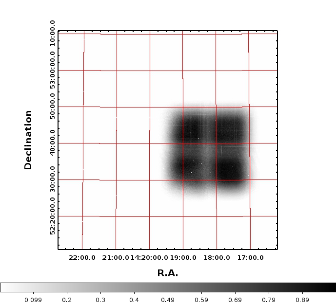
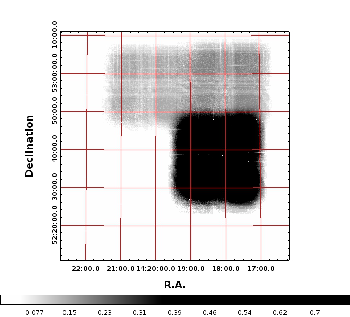
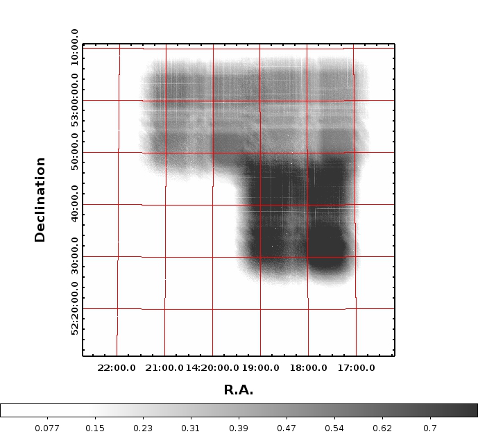
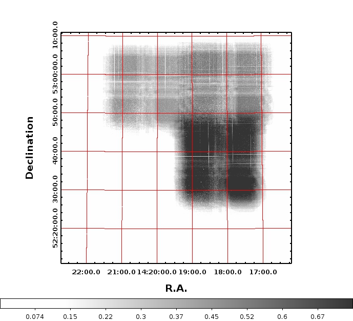
Figure 4 displays the exposure-time maps for the 11° CFHTLS-D3 field of view, and for the different near-IR filters. We note the difference in the total exposure times between the WUDS (deep) region and the extended region of WIRDS. Table 3 summarizes the number of sources detected in the different areas, for the different filters and detection images. Table 1 also presents the 3 limiting magnitudes achieved in the different filters within 1.3″diameter aperture (point sources). Completeness and depth achieved by WUDS are discussed below (see Sect. 5.1).
5 Characterization of the photometric survey
In this Section we characterize the properties of the WUDS photometric catalogs in different ways. Completeness and depth are estimated based on realistic simulations of stars and galaxies. Number counts are obtained in the near-IR bands and compared to previous findings.
| Area | |||||||
|---|---|---|---|---|---|---|---|
| (1) | AB | AB | AB | AB | |||
| WUDS | 77715 | 91340 | 59552 | 66623 | 34832 | 29841 | |
| 66479 | 79526 | 66627 | 72960 | 35791 | 30655 | ||
| 49920 | 57574 | 46185 | 49089 | 31900 | 28088 | ||
| WIRDS | - | 82200 | 35999 | 46225 | 21721 | - | |
| - | 86985 | 48063 | 65858 | 21706 | - | ||
| - | 41637 | 31759 | 36056 | 18371 | - |
5.1 Completeness and depth
The completeness of the WUDS survey has been estimated through simulations of stars and galaxies based on the STUFF and SKYMAKER softwares. Simulated samples of stars/galaxies have been randomly added to real images after masking of objects detected in the stacks, with the appropriate PSF convolution. These sources are then detected with SExtractor, using the same extraction parameters as for science images, therefore the completeness levels are directly obtained as a function of magnitude in the different bands. These values are reported in Tab. 1. The difference between the completeness levels in regions with the highest exposure time (90% ) and regions with smaller exposure times, for instance regions with 70% and 50% exposure time, is typically 0.08 and 0.13 magnitudes worse respectively. Therefore, given the geometry of the survey, the search for optical dropouts is limited in practice to regions with at least 50% of the total exposure time in the final stack (see Tab. 1). This means that the detection level does not change dramatically across the surveyed field.
The typical depth of the WUDS data reaches between 26.8 in and , and 26 in and Ks (AB, 3 in 1.3″aperture), for a completeness level of 80% at 26 and and Ks25.2, and excellent seeing values for the final stacks (ranging between 0.55 and 0.65 arcsec). The corresponding depth of the CFHTLS-D3 images in this region ranges between 28.6 and 29 in , 28.2 in and 27.1 in (same S/N ratio and aperture).
The price to pay for the low detection threshold used in this survey is an enhanced fraction of spurious detections, increasing with magnitude. As explained in Sect. 5.2 below, we have estimated this contamination using the same detection scheme on “negative” images and, in addition, all high-z candidates have been manually inspected. Based on these results, we have estimated that our catalogs are robust (in the sense that they are not dominated by false-positive detections in the near-IR images) up to AB 25.5 in and , and AB24.75 in and , irrespective of the detection image. The number of sources detected in the different areas, with magnitudes brighter than these limits are reported in Table 3, for the different filters and detection images.
5.2 Number counts
Galaxy number counts have been obtained in the four bands of WUDS and compared to the literature, as a consistency check for the calibration of the present data set. The separation between stars and galaxies is based on the SExtractor stellarity index99 9 This index ranges between 0.0 for extended sources and 1.0 for unresolved ones (Bertin & Arnouts, 1996, see).. Since the reliability of this index for galaxies diminishes toward the faintest magnitudes, we have applied this selection up to a S/N10 in the detection images, with galaxies selected by imposing a SExtractor stellarity index <0.9. These threshold values are based on straightforward simulations, using the same approach as for the determination of the completeness levels in Sect. 5.1.
Figure 5 displays the resulting number counts in the four bands of WUDS, as compared to previous findings from the literature (Cristóbal-Hornillos et al., 2003; Cristóbal-Hornillos et al., 2009; Laigle et al., 2016, e.g.,), without any correction for incompleteness. The detection image was for and bands, whereas it was for and . The 50% completeness levels for point sources coincide with the drop in number counts in the WUDS area. Compact sources with magnitudes brighter than 17.7 in , 18.1 in , 17.2 in and 17.6 in are affected by saturation. Although there is some scatter toward the bright end (AB20), there is a good agreement with previously published results, in particular Bielby et al. (2012).
The detection scheme described above was optimized to identify faint and compact sources (see Sect. 5.1). Therefore, a large fraction of spurious detections was expected in the near-IR bands, increasing toward the faintest magnitudes. In order to evaluate the incidence of this effect, we have applied an identical scheme for source detection as described in Sect. 5.1 to negative images obtained by multiplying the original stacks by , to blindly extract these spurious non-astronomical signal. The result of this procedure is also shown in Fig. 5 (open dots). The structure of the noise in these negative images is somewhat different with respect to the astronomical ones, in the sense that an excess of faint and compact sources appears toward the faintest magnitudes. As seen in Fig. 5, this systematic trend and the dominance of false positives start close to the 50% completeness levels in WUDS. The reason for this trend, which is also observed in other similar surveys (e.g., public CLASH data from HST), is not clear. It could be due to the drizzling and resampling procedure. For this reason, we did not try to use these negative counts to correct our results, but as an indication of the flux level at which severe contamination is expected. In practice, we have limited the detection samples to magnitudes reported in Table 3, where contamination is not expected to dominate. In addition, all the high-z candidates presented in this paper and in Paper II have been manually inspected to remove obvious spurious sources.
Regarding the comparison with previous findings on near-IR counts, our results are fully consistent with Cristóbal-Hornillos et al. (2003), Cristóbal-Hornillos et al. (2009) and Laigle et al. (2016) at m20, whereas a larger dispersion is observed for brighter sources as expected. WUDS is still deeper than UltraVISTA-DR2 survey in the -band (Laigle et al., 2016). The change in the slope of the near-IR counts at AB19.5-20.0 is clearly visible in the -band, whereas it is less obvious in the other bands, and not present in the optical bands (Cristóbal-Hornillos et al., 2009; Eliche-Moral et al., 2006, e.g.,). This trend has been identified by several authors using models (e.g., Eliche-Moral et al., 2010; Prieto & Eliche-Moral, 2015, and the references therein) as the result of the late assembly by major-mergers of a substantial fraction of present-day massive early-type galaxies at 0.7z1.2, and inconsistent with a simple passive evolution since z2.


6 Data properties at low-
In this Section we assess the quality achieved in the computation of photometric redshifts based on these data, up to z1.5. We also use the SED-fitting approach to derive the properties of the near-IR selected galaxy population in this field in terms of redshift distribution and stellar masses.
6.1 Photometric redshifts
Photometric redshifts have been computed with the version v12 of the public code Hyperz (NewHyperz1010 10 http://userpages.irap.omp.eu/rpello/newhyperz/), originally developped by Bolzonella et al. (2000). This method is based on the fitting of the photometric Spectral Energy Distributions (SED) of galaxies. The accuracy of photometric redshifts ( ) is used here as a consistency check for the calibration of the whole data set, as well as for the characterization of the different high-z samples in WUDS.
The template library used in this paper includes 14 templates: eight evolutionary synthetic SEDs computed with the last version of the Bruzual & Charlot code (Bruzual & Charlot, 2003), with Chabrier IMF (Chabrier, 2003) and solar metallicity, matching the observed colors of local galaxies from E to Im types (namely a delta burst -SSP-, a constant star-forming system, and six -models with exponentially decaying SFR); a set of four empirical SEDs compiled by Coleman et al. (1980), and two starburst galaxies from the Kinney et al. (1996) library. Internal extinction is considered as a free parameter following the Calzetti et al. (2000) extinction law, with AV ranging between 0 and 3.0 magnitudes (E(B-V) in the range [0,0.75] mag).
Photometric redshifts have been computed in the range z[0,12] using two different priors in luminosity. The first one is the usual flat luminosity prior in redshift, that is a simple cut in the permitted range of luminosities for extragalactic sources, with absolute magnitudes in the range MB=-14,-23. The second one is a “soft” probability distribution as a function of redshift and magnitude, following Benítez (2000), encompassing the -band luminosity function derived by Ilbert et al. (2006b). This new option of NewHyperz computes a smooth probability distribution prior for each object as a function of redshift, the absolute magnitude MB being derived from the apparent magnitude which is closer to the rest-frame -band. The final probability distribution is given by the usual combined with the prior.
NewHyperz performs a minimization in the parameter space in the first pass, followed by a small correction for systematics trends as a function of obtained through the polynomial fit of the residuals between the best-fit redshift above and the true value for the spectroscopic sample described below, excluding outliers. These residuals encode our lack of precise knowledge on the overall system transmission as a function of wavelength. The procedure yields the best fit and model template for each source, as well as a number of fitting byproducts (e.g., absolute magnitudes in the different bands, normalized redshift probability distribution, error bars, secondary solutions, …). An interesting indicator of the goodness of the fit is provided by the integrated probability between 0.1, where stands for the best fit redshift, with the probability distribution normalized between z[0, 12]. Among the fitting byproducts is a rough classification of the rest-frame SED of galaxies into five different spectral types, according to their best fit with the simplest empirical templates given by Coleman et al. (1980) and Kinney et al. (1996): (1) E/S0, (2) Sbc, (3) Scd, (4) Im and (5) S (starbursts).
The photometric redshift accuracy has been estimated through a direct comparison between and secure spectroscopic samples publically available in the CFHTLS-D3 field, extracted from the DEEP Groth Streep Survey DR3 (Weiner et al., 2005b; Davis et al., 2003; Davis et al., 2007). Photometric and spectroscopic catalogs were blindly matched in ALPHA and DEC positions. Only objects with the highest spectroscopic redshift quality (ZQUALITY 3) were considered in this comparison, that is 3424(3409) galaxies in the entire WUDSWIRDS area based on () detection images. Magnitudes in this sample range between =18 and 24.4, with median value =22.4, corresponding to =17.0 – 24.8 with median value =21.9. Results based on detection are the same as for the -based catalog. We have also considered the 3828 galaxies extracted form the detection image. Figure 6 displays the comparison between photometric and spectroscopic redshifts based on the detection image across the entire field, and the same restricted to the WUDS area, that is with photometry including -band data and 1651 spectroscopic sources.
Table 4 presents a summary of the quality achieved in this survey based on the usual statistical indicators, namely , , the median of , the normalized median absolute deviation (defined as = 1.48 median , which is less sensitive to outliers), and the percentage of outliers. These results are based on SExtractor MAG_AUTO magnitudes. Outliers are defined here as sources with . As shown in the table, the dispersion is below or on the order of in all cases based on the usual indicators, and the percentage of outliers ranges between 4 and 5% for the entire field, improving to 3-4% for the WUDS area, the results being slightly better for the near-IR selected samples. The same trends are also seen in Fig. 6, although the difference is small and hardly significant. The correction for systematic trends mentioned above is included in the results presented in Table 4 and Fig. 6. When this correction is not included, the results on the dispersion are worse by to 0.006 depending on the sample and indicator, whereas the median bias is up to a factor of 10 larger.
(1) Flat prior
(2) LF prior
(3) Median
| Detection | (all) | (all) | ||
|---|---|---|---|---|
| (1) | (2) | (1) | (2) | |
| 0.047 | 0.048 | 0.051 | 0.050 | |
| 0.031 | 0.031 | 0.032 | 0.032 | |
| Median (3) | 0.0016 | 0.0017 | -0.0017 | -0.0012 |
| 0.043 | 0.043 | 0.046 | 0.045 | |
| Outliers | 4.4% | 4.4% | 4.9% | 4.9% |
| Detection | (WUDS) | (WUDS) | ||
| (1) | (2) | (1) | (2) | |
| 0.047 | 0.047 | 0.049 | 0.049 | |
| 0.030 | 0.030 | 0.031 | 0.031 | |
| Median (3) | 0.0005 | 0.0007 | 0.0007 | 0.0007 |
| 0.042 | 0.042 | 0.044 | 0.045 | |
| Outliers | 2.9% | 2.8% | 3.8% | 3.9% |
The availability of near-IR filters helps improving the accuracy beyond 1.3, where the 4000Å break goes out of the filter and the Lyman break is not yet detectable in the band. The main impact when including -band data is on the percentage of outliers. Unfortunately, only 3% of the spectroscopic control sample is found at 1.3. Results obtained with a flat luminosity prior are not significantly different from those achieved using a more aggressive prior based on the LF. Results based on seeing-matched aperture magnitudes taking the -band as a reference are significantly worse than those based on MAG_AUTO, with a dispersion increasing by 0.01 to 0.02 with respect to the values displayed in Table 4. The reason for this is that the improved sampling in the SED obtained for seeing-matched apertures is compensated by a worse S/N ratio in the photometry as compared to MAG_AUTO, the net effect being a lower quality in the photometric redshifts.
The final quality achieved for WUDS without further refinement is within the requirements for large cosmological surveys (Laureijs et al., 2011, e.g., Euclid,), and it is expected to be representative of the general behavior for other SED-fitting codes applied to these data. Indeed, the dispersion and the percentage of outliers are comparable to the ones obtained with a similar number of filters in this redshift domain, such as for the 22.524.0 -selected sample in the VIMOS VLT Deep Survey (VVDS) (Ilbert et al., 2006a), the Hubble Ultra Deep Field (Coe et al., 2006), or the COSMOS field (Mobasher et al., 2007), whereas a better accuracy could be achieved by using a wider filter set (Ilbert et al., 2009, see e.g.,).


6.2 Properties of the galaxy population
We have taken advantage from the SED-fitting byproducts obtained by NewHyperz when deriving , as described in Sect. 6.1, to characterize the properties of the galaxy population in the WUDS survey. These quantities have been computed based on the catalogs used to select high-z sources in Sect. 7 below. Hereafter in this section, we limit the sample to sources fainter than the saturation limits in all WUDS filters, with SExtractor stellarity index 0.9, and detected in at least two near-IR filters with magnitudes brighter than AB25.5 in and , and AB24.75 in and . As discussed in Sect. 5.2, these limits ensure that the sample is not dominated by spurious sources. The sample presented here contains 110(118) x 103 sources in both catalogs based on () detection images.
Figure 7 displays the photometric redshift distribution obtained for different -band selected samples in this survey. As expected, the distribution extends to higher redshifts with increasing magnitudes, with a clear drop in the distribution of galaxies at z3.5, when the 4000Å break enters the -band.

Stellar masses are among the quantities derived by the SED-fitting procedure, based on the best-fit model obtained with the Bruzual & Charlot code (Bruzual & Charlot, 2003), with Chabrier IMF (Chabrier, 2003) and solar metallicity. The parameter space is precisely the same used for . As discussed by Davidzon et al. (2013), stellar masses derived in this way depend very weakly on the parameter space used for SED-fitting, in particular the detailed star-formation histories. A rough classification for the rest-frame SED of galaxies is provided by NewHyperz using five arbitrary spectral types, according to their best fit with the simplest empirical templates in the local universe, namely (1) E/S0, (2) Sbc, (3) Scd, (4) Im and (5) Starbursts (see Sect. 6.1). We consider here as genuine “early-type” all galaxies with best-fit type (1), and all the others are considered as “late-type”. Following Pozzetti et al. (2010), we have determined the completeness in mass for the early and late-type galaxies respectively for a sample limited to 24.75. This was done by computing the mass it would have an early/late type galaxy at the center of each redshift bin if its apparent magnitude was =24.75. Figure 8 displays the distribution of stellar masses measured in the WUDS field as a function of redshift and galaxy types, together with the limiting mass corresponding to 24.75 for early and late-type galaxies. Error bars in this figure represent the dispersion within the sample for a typical 24.75 galaxy.
Several trends in Figure 8 deserve a specific comment. There is a systematic trend in the sense that the dispersion within the sample increases with redshift for a given spectral type. Uncertainties in the determination of individual stellar masses due to various degeneracies in the parameter space are expected to be typically below 0.2 dex up to z3.5, that is when the observed SED includes the 4000Å break, but the determination becomes hazardous beyond this redshift (see e.g., Pforr et al., 2013; Mitchell et al., 2013, for a detailed discussion). As seen in Figures 7 and 8, the population of galaxies beyond z3.5 strongly diminishes in our near-IR selected catalog, essentially because the region of the SED beyond the 4000Å break, tracing the “old” stellar population and the stellar mass, progressively moves beyond the reddest band (). This trend is expected given the limited wavelength coverage of WUDS (the reddest band is ). For this reason, the completeness limit displayed in Figure 8 for early-type galaxies stops at z3.5, whereas it is given as an indication only for late-type galaxies beyond this limit, given the uncertainties associated to the stellar mass determination beyond this redshift.
Although WUDS catalogs were built to fulfill the needs of our primary science goal around the z4.5 population, they could also be advantageously used for studies at low and mid-z, in particular for the stellar-mass preselection of galaxies for spectroscopic studies. Up to z3.5, early-type galaxies can be reliably identified and used for statistical purposes down to log(M∗/M)10.51.0 (completeness for a typical =24.75 galaxy), whereas we expect to detect late-type galaxies down to log(M∗/M)9.90.60. Beyond this limit in redshift, stellar masses cannot be properly determined.

7 Galaxies at z4.5 – 7
7.1 Selection Criteria
We have used two different methods to select high-z galaxies. The first one is the usual three-band dropout technique applied to a combination of WUDS data and deep optical data from the CFHTLS-D3, that is a photometric catalog including the nine filter-bands (). Different redshift intervals have been defined using an appropriate combination of filters. The second method is based on pure photometric redshifts and probability distributions, taking full advantage from the wide wavelength coverage. In all cases, a S/N higher than 5 was requested in the filters encompassing the rest-frame UV, irrespective of the detection image, together with a non-detection (2 level) in all filters bluewards from the Lyman limit. In this respect, CFHTLS-D3 data are particularly useful to provide robust non-detection constraints for candidates at z4.5 – 7. Detailed selection criteria are provided below. In the subsequent sections we compare the samples selected and the global properties derived when using different approaches.
Regarding the dropout technique, three selection windows have been used to cover the z4.5 – 7 interval, as shown in Fig. 9:
- (a)
, and . This window selects -dropout candidates in the z4.5 – 5.3 interval, as shown in the top panel of Fig. 9. This selection window is analogous to the one used in the literature to isolate RIz LBGs in the same redshift range from foreground interlopers and galactic stars (Ouchi et al., 2004; Yoshida et al., 2006; Bouwens et al., 2015; Ono et al., 2017, see e.g.,).
- (b)
and , a window selecting -dropout candidates in the z5.3 – 6.4 interval, as shown in the mid panel of Fig. 9. This selection window is analogous to the one used in other studies previous (Bouwens et al., 2007; Bouwens et al., 2015, see e.g.,), but less strict than in the selection conducted by Willott et al. (2013).
- (c)
and . This window is intended to select -band dropouts in the z6.3 – 7.2 interval, as shown in the bottom panel of Fig. 9. The field of view in this case is limited to the WUDS region (see Table 1 and Fig. 4). The use of deep -band images is particularly useful in this redshift interval and it is rarely found in the literature excepted for HST data (Bouwens et al., 2011; Bouwens et al., 2015, see e.g.,).
Photometric redshifts and associated probability distributions have several advantages with respect to the three-band dropout technique (McLure et al., 2009; Finkelstein et al., 2015, see e.g.,). Although the later have proven to be successful in isolating high-z galaxies, a significant fraction of the whole population could have been excluded due to different reasons (e.g., older stellar populations, redder colors, …). SED fitting analysis is particularly useful for objects lying close to the boundaries of the color-color selection boxes. The selection criteria in this case are simply given by magnitude-selected catalogs (at least 5 in the filter encompassing the rest-frame UV), and a detection below 2 level in all filters bluewards with respect to 912 rest-frame. We have adopted the redshift probability distributions (hereafter ) obtained when applying the procedure described in Sect. 6.1. Given the selection based on rest-frame UV, the final sample is still expected to be biased toward star-forming and low-reddening galaxies.


| C1 | C2 | ||
| () | () | () | |
| Criteria | N | N | N |
| dropout (raw) | 2016 | 2591 | 2797 |
| z4.5 - 5.3 CC window | 863 | 1085 | 1205 |
| CC window corrected | 817 | 711 | - |
| dropout (raw) | 166 | 134 | |
| dropout (corrected) | 91 | 71 | |
| z5.3 - 6.4 CC window | 98 | 66 | |
| CC window corrected | 48 | 32 | |
| dropout (raw) | 212 | 256 | |
| dropout (corrected) | 142 | 132 | |
| z6.3 - 7.2 CC window | 36 | 30 | |
| CC window corrected | 14 | 11 |
7.2 Samples of galaxies at z4.5 – 7
The results obtained when applying the selection criteria described in Sect. 7.1 are presented in this section. Table 5 summarizes these results for the different redshift bins and selection criteria. In all cases we compare the samples extracted from the different detection images and corresponding catalogs, namely , C1 () and C2 (), and we restrict the selection area to the region covered by all filters involved in the detection with at least 50% of the total exposure time, excluding noisy areas (e.g., around bright stars). The following samples have been selected:
- (a)
dropout sample: A S/N higher than 5 is requested in and , together with a non-detection at less than 2 level in and , and . This blind selection provides 2600(2800) sources in C1(C2) respectively, over the 1200 arcmin2 field covered by near-IR data. Among them, 1100(1200) are included within the color-color window for the selection of candidates in the z4.5 – 5.3 interval. When using the detection image instead, 2000 sources are found over the same area, 863 of them within the color-color window. An average(median) value of =4.82(4.80) is found for this sample. Although the number of sources is smaller in the later case, the -selected sample contains a smaller fraction of false positives, as discussed below. This -selected sample will be used to derive the LF at z5.
- (b)
dropout sample: A S/N higher than 5 is requested in and , together with a non-detection at less than 2 level in , and , and . In this case the selection is only applied to the deep WUDS region covered by the band. These criteria blindly select 166(134) sources in C1(C2) over 390 arcmin2, and among them 98(66) objects included within the color-color window for the selection of candidates at z5.3 – 6.4. An average(median) value of =5.84(5.89) is found for this sample.
- (c)
dropout sample: A S/N higher than 5 is requested in and , together with a non-detection at less than 2 level in , , and , and . As in the previous case, only the WUDS region is used for this selection. When these criteria are blindly applied, 655(627) objects are selected in C1(C2). However, there is a difference between this sample and the previous ones due to the depth in the -band filter, which is 0.5 magnitudes shallower than the -band, as shown in Table 1. A robust selection based on is only achieved for objects with . When introducing this additional constraint, the final sample reduces to 212(256) objects in C1(C2) over 390 arcmin2, and among them only 36(30) objects are included within the color-color window for the selection of candidates at z6.3 – 7.2. An average(median) value of =6.83(6.87) is found for this sample.
We have also corrected for obvious spurious sources in the above catalogs by visual inspection carried out by two different observers. The percentage of spurious sources in the dropout sample is smaller than for the and dropouts, reaching only 5% for the detection image. This trend was somewhat expected because a good S/N was requested in both and , that is at least two visible bands, together with a detection on the near-IR images for C1 and C2, making the selection of spurious signal highly unlikely. On the contrary, the contamination is expected to be much higher when the selection is essentially based on near-IR images, with extraction in double-image mode and a low detection threshold, together with a poor detection or not-detection in the optical bands. The presence of spurious sources is indeed larger in this case, reaching between 30 and 60% of the sample, depending on the detection image and selection window. Therefore we have visually inspected and validated all objects used in the subsequent analysis. Corrected counts are reported in Table 5 together with the raw counts, to illustrate this effect. A detailed study of the dropout sample is presented in Paper II, in particular the contamination affecting the z7 sample.
7.3 Luminosity functions at z5 and z6
In this section we derive the UV LF at 1500 Å in two different redshift bins around z5 and z6, based on the near-IR-selected samples of WUDS reported in Table 5. The results obtained on the LF at z7, as well as the evolution of the UV LF between z 4.5 and 9, are presented and discussed in Paper II.
For each redshift bin, two different approaches and samples have been used to derive the LF. In one hand, the complete dropout and dropout catalogs, corrected for spurious detections, without any additional color-selection, are used to compute the LF based on photometric redshifts probability distributions (). On the other hand, we have used the (corrected) subsamples included within the corresponding LBG color-color selection windows. These two different approaches and samples are widely used in the literature.
Number density values in luminosity bins have been computed using the method (Schmidt, 1968, see e.g.,). The bootstrap approach developed by Bolzonella et al. (2002) has been adopted to compute the LF data points, that is number density values and confidence intervals. This method is based on blind photometric redshifts and associated probability distributions . For a given redshift interval, 1000 realizations of each catalog have been performed; for each realization of the catalog and for each object, a random value of the photometric redshift was sorted out according to its . This procedure takes into account by construction the existence of degenerate solutions in redshift for a given source. The number of realizations of each catalog is large enough to ensure that the LF results do not depend on the number of realizations.
Absolute magnitudes in the UV at 1500Å (M1500) are derived from the photometric SED datapoints overlapping this wavelength for a given (photometric) redshift. We have checked that there is no significant difference in the LF results when using the closest filter-band, assuming a flat continuum, or the precise flux at rest-frame 1500Å for the best-fit model instead.
Number densities have been corrected for photometric incompleteness depending on the selection bands, according to Sect. 5.1. For samples selected in LBG windows, an additional multiplicative correction was applied to include the effect of color selection as a function of redshift and magnitude (S/N ratio) in the detection filter encompassing the 1500Å rest-frame. The shape of this later correction was obtained through simulated catalogs, each one containing 4 105 objects, fully covering the redshift windows 4.5,5.5 and 5.5,6.5. These catalogs are based on the same templates used to define the selection windows, with magnitudes and corresponding photometric errors sorted to uniformly sample the actual range of magnitudes in the WUDS survey. We have then applied to these simulated catalogs the same color selection as for real data. The correction factor in a given redshift and magnitude bin is simply derived as the ratio between the number of galaxies in the input sample and number actually retrieved by the selection process. Also the redshift interval defined by dropout and dropout selections is actually narrower than the nominal z=1. In order to facilitate the comparison between the different samples, we have used a fixed z=1 in all cases assuming a uniform number density of sources. Therefore, in the following, number densities are given for redshift bins 4.5,5.5 and 5.5,6.5 respectively for convenience, and also to facilitate the comparison with other surveys.
LF values have been computed using regularly spaced bins in luminosity of =0.125 at z5 and =0.250 at z6, excepted for the first (brightest) bins, arbitrarily set to =0.25 mags or 0.50 to improve statistics. Note that the number of sources used in the blind photometric redshift approach is larger than in the LBG color-color window (because less restrictive; see Table 5), allowing us to better sample the LF at z6. The fact that no source was detected at magnitudes brighter than M and respectively for and dropouts has been used to determine upper limits for the bright end of the LF.
It should be noted that results obtained at z5 strongly depend on the detection image used for the dropout selection. In the following and for a sake of consistency, we use the catalogs derived from detection images encompassing the rest-frame 1500Å (see discussion below), that is at z5 and C1 at z6. Tables 6 and 7 summarize the LF data points at z5 and z6 respectively, for the different detection catalogs. In all cases, error bars corresponding to 68% (1) confidence levels resulting from the bootstrap process are combined together with an estimate of Poisson uncertainties and field-to-field variance derived from the public cosmic variance calculator by Trenti & Stiavelli (2008). These later contributions clearly dominate the error budget, excepted for the brightest M luminosity bins.
Tables 6 and 7 present the LF points derived at z5 and z6 using the two approaches/samples to compute the LF, namely photometric redshifts applied to blindly selected dropout samples, and the classical LBG color-preselected samples. Results are found to be consistent, in general at better than 1 level, the largest deviations being observed for the faintest luminosities at z6. As discussed below, these results are also in agreement with previous findings at the same redshifts, as if photometric redshifts and associated probability distributions could be safely used for these purposes on the dropout samples, without introducing more sophisticated and to a certain extent dangerous cuts in color space. This statement requires some additional discussion (see below).


A subsequent maximum-likelihood fit of data points has been performed to the analytic Schechter function (Schechter, 1976) as follows:
| (1) |
based on a simple least-squares minimization, assuming that the Schechter function provides a good representation of data. The fit has been obtained separately for data points derived through the classical LBG color-selection window and blind photometric redshifts to facilitate the comparison with previous findings.
Our data being essentially sensitive to the normalization and M⋆, we have studied the influence of the slope in two different ways: by adding data points from the literature toward the faintest luminosities, and by setting the slope of the LF. First, we completed our step-wise data points toward the faint edge using the LF estimates by Bouwens et al. (2015) at z5 and z6, based on deep HST imaging. A good-quality fit was obtained at z5, with stable and consistent results for both the LBG color-selection window and blind photometric redshifts, also consistent with the slope value derived by Bouwens et al. (2015). On the contrary, at z6 a good-quality fit could not be achieved for the enlarged data set based on the LBG color-selection window, but only for the photometric redshift LF data (for which the sampling of the LF is better, as shown in Table 7). Therefore, in a second step, we imposed a constant slope for the LF following Bouwens et al. (2015) (also based on LBG color window) while leaving the normalization and M⋆ free. In this case, a good fit was also achieved at z6, yielding consistent results for both the LBG color-selection window and blind photometric redshifts. The effect of imposing a constant slope for the LF was studied by using also the steeper value from the Finkelstein (2016) review and from Livermore et al. (2017) in lensing fields, both studies being based on photometric redshifts. As seen in Table 8, our results for and L⋆ are in good agreement with those previously found by Finkelstein (2016) and Livermore et al. (2017) when imposing the same value of (see below).
Our best fit to WUDS data-sets yields the results summarized in Table 8, namely (8.20)10-4 Mpc-3, M-20.980.03 mag, and -1.74 0.02 for z5, and (7.5)10-4 Mpc-3 and M-20.580.022 mag with fixed -1.87 for z=6, for the LBG color-selection window. Figure 10 and 11 display the data points adopted for the LBG color-selection window for z5 and z6 respectively, together with the best-fit representation by a Schechter function as discussed above. Our results confirm a slight evolution in the UV LF between z5 and z6, consistent with a dimming of both and L⋆.
Oddly, when comparing our results at z6 with previous findings in Fig. 11, at first glance they are found to be more consistent with Bouwens et al. (2015) for the blind photometric redshift approach, whereas they are more consistent with Finkelstein et al. (2015) for the LBG color-selection window, while the opposite trend would have been expected. In reality, as seen in Table 8, the results of the Schechter fit derived from both the color-selection window and the photometric redshift approaches are fully consistent within the error bars with Bouwens et al. (2015) when imposing the same slope -1.87, the larger differences being in the normalization. When imposing a steeper slope -2, as found by Finkelstein (2016) or Livermore et al. (2017) based on the photometric redshift approach, then the results of the fit are fully consistent with their findings regarding and L⋆. In other words, the results obtained on L⋆ and the normalization seem to be more sensitive to the imposed value for the slope rather than to the approach/method used to select the samples.
It is worth to mention that the difference between the LF points derived from the two samples/approaches defined within the same WUDS field provides an estimate of the systematic uncertainties related to the selection function, that are not necessarily taken into account in the literature (see Finkelstein, 2016, for a review), meaning that the final errors on the LF points and fits could be systematically underestimated. In this study, the LF points derived at z5 are fully consistent within the error bars between the two approaches, making the LF parameters particularly robust. At z6, the difference between the two approaches is negligible for the brightest region, that is smaller than 30% up to M -21.5 (similar or smaller than the error bars), whereas at lower luminosities the photometric redshift approach yields 0.3 higher in average. When quadratically combining these differences with the current error bars, as if they were the expression of a systematic error, we find that the fit results for the LF are very slightly modified (e.g., 0.01 for the slope when it is let free, 0.02 for M1500, and a negligible amount for the normalization, the error bars on these parameters increasing by only 10%). This means that there is indeed a systematic effect to take into account, but it is not strong enough here to modify the conclusions of this study.
| drop Photometric Redshifts | LBG color window | ||||
|---|---|---|---|---|---|
| M1500 | M1500 | ||||
| [AB mag] | [Mpc-3 mag-1] | [Mpc-3 mag-1] | [AB mag] | [Mpc-3 mag-1] | [Mpc-3 mag-1] |
| -22.8750.500 | 1.23 10-7 | -22.8750.500 | 1.23 10-7 | ||
| -22.125 0.250 | 1.86 10-5 | 0.77 10-5 | -22.125 0.250 | 2.57 10-5 | 0.97 10-5 |
| -21.625 0.250 | 5.86 10-5 | 2.12 10-5 | -21.625 0.250 | 7.90 10-5 | 2.10 10-5 |
| -21.250 0.125 | 1.73 10-4 | 0.44 10-4 | -21.250 0.125 | 1.58 10-4 | 0.42 10-4 |
| -21.000 0.125 | 2.71 10-4 | 0.68 10-4 | -21.000 0.125 | 2.59 10-4 | 0.61 10-4 |
| -20.750 0.125 | 7.86 10-4 | 1.60 10-4 | -20.750 0.125 | 4.13 10-4 | 0.87 10-4 |
| -20.500 0.125 | 9.51 10-4 | 1.94 10-4 | -20.500 0.125 | 7.19 10-4 | 1.36 10-4 |
| drop Photometric Redshifts | LBG color window | ||||
|---|---|---|---|---|---|
| M1500 | M1500 | ||||
| [AB mag] | [Mpc-3 mag-1] | [Mpc-3 mag-1] | [AB mag] | [Mpc-3 mag-1] | [Mpc-3 mag-1] |
| -22.375 0.50 | 4.19 10-7 | -22.375 0.50 | 4.19 10-7 | ||
| -22.75 0.25 | 2.25 10-6 | 2.41 10-6 | -22.25 0.50 | 9.07 10-6 | 4.0 10-6 |
| -22.25 0.25 | 8.56 10-6 | 5.08 10-6 | -21.50 0.25 | 3.51 10-5 | 1.24 10-5 |
| -21.75 0.25 | 1.80 10-5 | 0.82 10-5 | -20.87 0.25 | 8.72 10-5 | 2.62 10-5 |
| -21.25 0.25 | 1.15 10-4 | 0.30 10-4 | |||
| -20.75 0.25 | 1.82 10-4 | 0.47 10-4 | |||
7.4 Discussion. Comparison with previous findings
The LF at z5 and z6 has been the subject of various studies during the last ten years (Yoshida et al., 2006; Bouwens et al., 2007; McLure et al., 2009; Su et al., 2011; Bouwens et al., 2012; Willott et al., 2013; Finkelstein et al., 2015; Bouwens et al., 2015; Finkelstein, 2016; Livermore et al., 2017; Ono et al., 2017, see e.g.,). Although detailed results on the evolution of the LF will be presented in Paper II, the comparison between the present results and previous findings is important to assess the quality of the survey. WUDS covers an interesting region in luminosity between the exponential and power-law-dominated regimes of the LF. WUDS has been designed to provide constraints on the brightest part of the LF at high-z, in particular on M⋆ and , and it is much less sensitive to the value of , as discussed in Sect. 7.3. We compare in Table 8 the LF parameters obtained in this survey at z5 and z6 with current findings in the literature, in complement to Fig. 10 and 11.
As expected by construction, the best-fit values when the slope is let free are fully consistent with Bouwens et al. (2015) because we used their data points to complete the LF toward the faintest luminosities. It should be mentioned however that, at z6, our faintest bins are in agreement with Bouwens et al. (2015) for the photometric redshift “blind” approach, whereas a better agreement is found with Finkelstein et al. (2015) when using the LBG color-window, as seen in Fig. 11, while the opposite trend would have been expected. As discussed in Sect. 7.3, given the error bars, the results obtained on and L⋆ seem to be more sensitive to the value imposed for the slope rather than to the method used to select the samples.
With the clarifications given above, our results are consistent with a small evolution of both M⋆ and between z5 and z6. There is also a good agreement in general between our M⋆ and values and recently published results within the error bars. At z6 this is true provided that the same value for the slope is imposed. At z5, the present combined determination of M⋆ and is more accurate then previous findings due to a better statistics in the intermediate-luminosity regime. Regarding the value of the slope at this redshift, we confirm the value proposed by Bouwens et al. (2015), and we are marginally consistent with Finkelstein et al. (2015) and Ono et al. (2017). Our results lend support to higher determinations than usually reported at z6, but still consistent with the latest findings by Bouwens et al. (2015), Finkelstein (2016), and Ono et al. (2017). Of particular interest is the comparison with Willott et al. (2013) at z6 (Table 3 in their paper), because it was based on CFHTLS-Deep data partly covering the WIRDS area. Even though the selection criteria are not the identical (see Sect. 7.1), and their LF was obtained at 1350 instead of 1500 Å , the global fit to our data as well as the number densities obtained in the present paper are consistent with their results. Given the error bars, our results are consistent with an evolution in L⋆, as expected if the UV luminosity of galaxies follows the assembly of host dark matter halos (Bouwens et al., 2008, see e.g.,), without excluding an evolution on the global normalization, as reported for instance by Bouwens et al. (2015). A direct comparison is recognized to be difficult given the degeneracy between the Schechter parameters on one hand, and the differences in the methods and samples used to build the LF on the other hand.
| z5 | |||
|---|---|---|---|
| References | M⋆ | ||
| [FUV AB mag] | [10-4 Mpc-3] | ||
| WUDS (LBG color window) | -1.74 0.02 | -20.980.03 | 8.20 |
| WUDS (Photometric Redshifts) | -1.74 0.04 | -21.020.08 | 8.00 |
| McLure et al. (2009) | -1.66 0.06 | -20.730.11 | 9.40.19 |
| Finkelstein et al. (2015) | -1.670.06 | -20.81 | 8.95 |
| Bouwens et al. (2015) | -1.760.06 | -21.170.12 | 7.4 |
| Ono et al. (2018) | -1.600.06 | -20.950.06 | 10.7 |
| z6 | |||
| References | M⋆ | ||
| [FUV AB mag] | [10-4 Mpc-3] | ||
| WUDS (LBG color window) | -1.87 (fixed) | -20.580.22 | 7.5 |
| WUDS (Photometric Redshifts) | -1.840.09 | -20.770.20 | 6.5 |
| WUDS (Photometric Redshifts) | -1.87 (fixed) | -20.830.22 | 5.8 |
| WUDS (Photometric Redshifts) | -1.91 (fixed) | -20.800.30 | 5.7 |
| WUDS (Photometric Redshifts) | -2.10 (fixed) | -21.20 | 2.45 |
| McLure et al. (2009) | -1.710.11 | -20.040.12 | 1.800.50 |
| Su et al. (2011) | -1.870.14 | -20.250.23 | 1.77 |
| Finkelstein et al. (2015) | -2.020.10 | -21.13 | 1.86 |
| Bouwens et al. (2015) | -1.870.10 | -20.940.20 | 5.0 |
| Bowler et al. (2015) | -1.88 | -20.77 | 5.7 |
| Finkelstein (2016) | -1.91 | -20.79 | 4.26 |
| Livermore et al. (2017) | -2.100.03 | -20.826 | 2.254 |
| Ono et al. (2018) | -1.860.07 | -20.900.07 | 5.5 |
8 Conclusions and Perspectives
In this paper we have introduced and characterized the WIRCam Ultra Deep Survey (WUDS), a 4-band near-IR photometric survey covering 400 arcmin2 on the CFHTLS-D3 field (Groth Strip). This public survey was specifically tailored to set strong constraints on the cosmic SFR and the UV luminosity function brighter or around in the z6-10 domain.
Regarding the properties of the data at low-, and according to the estimates presented in this article, WUDS should allow the users to detect early-type galaxies with stellar masses down to log(M⋆/M)10.51.0, and late-type galaxies down to log(M⋆/M)9.90.60 up to z3.5. The quality of the photometric redshifts achieved for the WUDS survey is comparable to the one obtained by other large surveys when using a similar number of filters and a similar depth.
As part of this effort, we have focused in this article on the selection of galaxy samples at z4.5 – 7 and the determination of the UV LF at z5 and z6, taking advantage from the deep optical data available from the CFHTLS-Deep Survey. We have also extended the research to an adjacent shallower area of 1000 arcmin2 extracted from the WIRDS Survey, and observed in three near-IR bands. Using two different approaches, the classical LBG color-selection technique and photometric redshifts blindly applied to dropout samples, we have selected high-z galaxies and computed the UV LF. At z5, the combined determination of M⋆ and is more accurate then previous results due to a better statistics in the intermediate-luminosity regime. The evolution in the UV LF between z5 and z6 is consistent with a small dimming in both and L⋆. These results are consistent with previous findings in terms of the M⋆ and values, knowing that WUDS covers a particularly interesting interval at intermediate luminosities.
The selection and combined analysis of different galaxy samples at z7 will be presented in a forthcoming paper, as well as the evolution of the UV luminosity function between z 4.5 and 9 (Laporte et al., submitted to A & A, Paper II). Photometric data and catalogs will be set publicly available at the http://wuds.irap.omp.eu/ web site.
WUDS is intended to provide a robust database in the near-IR for the selection of targets for the Galaxy Origins and Young Assembly (GOYA) Survey. GOYA is a scientific program to be developed mainly using the guaranteed time of the international consortium building EMIR, a wide-field, near-IR spectrograph currently installed in the Nasmyth focus of the Spanish 10.4m GTC at Canary Islands1414 14 http://www.gtc.iac.es (Garzón et al., 2006). The GOYA project addresses the formation and evolution of galaxies, in particular the structure, dynamics and integrated stellar populations of galaxies at high redshift (Guzman, 2003; Balcells, 2003; Balcells, 2007; Domínguez-Palmero et al., 2008, see e.g.,).
Acknowledgements.
Part of this work was supported by the French CNRS, the French Programme National de Cosmologie et Galaxies (PNCG) of CNRS/INSU with INP and IN2P3, co-funded by CEA and CNES. We acknowledge support from the Spanish Programa Nacional de Astronomía y Astrofísica under grant AYA 2006-02358 and the Swiss National Science Foundation. Partially funded by the Spanish MEC under the Consolider-Ingenio 2010 Program grant CSD2006-00070: First Science with the GTC (http://www.iac.es/consolider-ingenio-gtc/). This work recieved support from Agence Nationale de la recherche bearing the reference ANR-09-BLAN-0234, and from the ECOS SUD Program C16U02. This work has been carried out thanks to the support of the OCEVU Labex (ANR-11-LABX-0060) and the A*MIDEX project (ANR-11-IDEX-0001-02) funded by the "Investissements d’Avenir" French government program managed by the ANR. NL acknowledges financial support from European Research Council Advanced Grant FP7/669253. JG and NC acknowledge financial support from Spanish MINECO (AYA2016-75808-R). MB acknowledges support from AYA grant 2009-11139. This paper is based on observations obtained with WIRCam, a joint project of CFHT, Taiwan, Korea, Canada, France, and the Canada-France-Hawaii Telescope (CFHT) which is operated by the National Research Council (NRC) of Canada, the Institute National des Sciences de l’Univers of the Centre National de la Recherche Scientifique of France, and the University of Hawaii. Funding for the DEEP2 survey has been provided by NSF grants AST95-09298, AST-0071048, AST-0071198, AST-0507428, and AST-0507483 as well as NASA LTSA grant NNG04GC89G.References
- Balcells (2003) Balcells, M. 2003, in Revista Mexicana de Astronomia y Astrofisica, vol. 27, Vol. 16, Revista Mexicana de Astronomia y Astrofisica Conference Series, ed. J. M. Rodriguez Espinoza, F. Garzon Lopez, & V. Melo Martin, 69–72
- Balcells (2007) Balcells, M. 2007, in Revista Mexicana de Astronomia y Astrofisica, vol. 27, Vol. 29, Revista Mexicana de Astronomia y Astrofisica Conference Series, ed. R. Guzmán, 126–128
- Benítez (2000) Benítez, N. 2000, ApJ, 536, 571
- Bertin & Arnouts (1996) Bertin, E. & Arnouts, S. 1996, A&AS, 117, 393
- Bielby et al. (2012) Bielby, R., Hudelot, P., McCracken, H. J., et al. 2012, A&A, 545, A23
- Bolzonella et al. (2000) Bolzonella, M., Miralles, J.-M., & Pelló, R. 2000, A&A, 363, 476
- Bolzonella et al. (2002) Bolzonella, M., Pelló, R., & Maccagni, D. 2002, A&A, 395, 443
- Bouwens et al. (2007) Bouwens, R. J., Illingworth, G. D., Franx, M., & Ford, H. 2007, ApJ, 670, 928
- Bouwens et al. (2008) Bouwens, R. J., Illingworth, G. D., Franx, M., & Ford, H. 2008, ApJ, 686, 230
- Bouwens et al. (2011) Bouwens, R. J., Illingworth, G. D., Oesch, P. A., et al. 2011, ApJ, 737, 90
- Bouwens et al. (2015) Bouwens, R. J., Illingworth, G. D., Oesch, P. A., et al. 2015, ApJ, 803, 34
- Bouwens et al. (2012) Bouwens, R. J., Illingworth, G. D., Oesch, P. A., et al. 2012, ApJ, 752, L5
- Bouwens et al. (2004) Bouwens, R. J., Thompson, R. I., Illingworth, G. D., et al. 2004, ApJ, 616, L79
- Bowler et al. (2015) Bowler, R. A. A., Dunlop, J. S., McLure, R. J., et al. 2015, MNRAS, 452, 1817
- Bruzual & Charlot (2003) Bruzual, G. & Charlot, S. 2003, MNRAS, 344, 1000
- Bunker et al. (2010) Bunker, A. J., Wilkins, S., Ellis, R. S., et al. 2010, MNRAS, 409, 855
- Calzetti et al. (2000) Calzetti, D., Armus, L., Bohlin, R. C., et al. 2000, ApJ, 533, 682
- Cassata et al. (2013) Cassata, P., Giavalisco, M., Williams, C. C., et al. 2013, ApJ, 775, 106
- Chabrier (2003) Chabrier, G. 2003, PASP, 115, 763
- Cimatti et al. (2002) Cimatti, A., Daddi, E., Mignoli, M., et al. 2002, A&A, 381, L68
- Coe et al. (2006) Coe, D., Benítez, N., Sánchez, S. F., et al. 2006, AJ, 132, 926
- Coe et al. (2013) Coe, D., Zitrin, A., Carrasco, M., et al. 2013, ApJ, 762, 32
- Coleman et al. (1980) Coleman, G. D., Wu, C.-C., & Weedman, D. W. 1980, ApJS, 43, 393
- Cowie et al. (1994) Cowie, L. L., Gardner, J. P., Hu, E. M., et al. 1994, ApJ, 434, 114
- Cristóbal-Hornillos et al. (2009) Cristóbal-Hornillos, D., Aguerri, J. A. L., Moles, M., et al. 2009, ApJ, 696, 1554
- Cristóbal-Hornillos et al. (2003) Cristóbal-Hornillos, D., Balcells, M., Prieto, M., et al. 2003, ApJ, 595, 71
- Davidzon et al. (2013) Davidzon, I., Bolzonella, M., Coupon, J., et al. 2013, A&A, 558, A23
- Davis et al. (2003) Davis, M., Faber, S. M., Newman, J., et al. 2003, in Society of Photo-Optical Instrumentation Engineers (SPIE) Conference Series, Vol. 4834, Society of Photo-Optical Instrumentation Engineers (SPIE) Conference Series, ed. P. Guhathakurta, 161–172
- Davis et al. (2007) Davis, M., Guhathakurta, P., Konidaris, N. P., et al. 2007, ApJ, 660, L1
- Domínguez-Palmero et al. (2008) Domínguez-Palmero, L., Balcells, M., Erwin, P., et al. 2008, A&A, 488, 1167
- Eliche-Moral et al. (2006) Eliche-Moral, M. C., Balcells, M., Prieto, M., et al. 2006, ApJ, 639, 644
- Eliche-Moral et al. (2010) Eliche-Moral, M. C., Prieto, M., Gallego, J., et al. 2010, A&A, 519, A55
- Finkelstein (2016) Finkelstein, S. L. 2016, PASA, 33, e037
- Finkelstein et al. (2012) Finkelstein, S. L., Papovich, C., Salmon, B., et al. 2012, ApJ, 756, 164
- Finkelstein et al. (2015) Finkelstein, S. L., Ryan, Jr., R. E., Papovich, C., et al. 2015, ApJ, 810, 71
- Garzón et al. (2007) Garzón, F., Abreu, D., Barrera, S., et al. 2007, in Revista Mexicana de Astronomia y Astrofisica, vol. 27, Vol. 29, Revista Mexicana de Astronomia y Astrofisica Conference Series, ed. R. Guzmán, 12–17
- Garzón et al. (2006) Garzón, F., Abreu, D., Barrera, S., et al. 2006, in Society of Photo-Optical Instrumentation Engineers (SPIE) Conference Series, Vol. 6269, Society of Photo-Optical Instrumentation Engineers (SPIE) Conference Series
- Garzón et al. (2016) Garzón, F., Castro, N., Insausti, M., et al. 2016, in Proc. SPIE, Vol. 9908, Ground-based and Airborne Instrumentation for Astronomy VI, 99081J
- Grogin et al. (2011) Grogin, N. A., Kocevski, D. D., Faber, S. M., et al. 2011, ApJS, 197, 35
- Guzman (2003) Guzman, R. 2003, in Revista Mexicana de Astronomia y Astrofisica, vol. 27, Vol. 16, Revista Mexicana de Astronomia y Astrofisica Conference Series, ed. J. M. Rodriguez Espinoza, F. Garzon Lopez, & V. Melo Martin, 209–212
- Ilbert et al. (2006a) Ilbert, O., Arnouts, S., McCracken, H. J., et al. 2006a, A&A, 457, 841
- Ilbert et al. (2009) Ilbert, O., Capak, P., Salvato, M., et al. 2009, ApJ, 690, 1236
- Ilbert et al. (2006b) Ilbert, O., Lauger, S., Tresse, L., et al. 2006b, A&A, 453, 809
- Illingworth et al. (2013) Illingworth, G. D., Magee, D., Oesch, P. A., et al. 2013, ApJS, 209, 6
- Kinney et al. (1996) Kinney, A. L., Calzetti, D., Bohlin, R. C., et al. 1996, ApJ, 467, 38
- Kneib et al. (2004) Kneib, J.-P., Ellis, R. S., Santos, M. R., & Richard, J. 2004, ApJ, 607, 697
- Koekemoer et al. (2011) Koekemoer, A. M., Faber, S. M., Ferguson, H. C., et al. 2011, ApJS, 197, 36
- Labbé et al. (2003a) Labbé, I., Franx, M., Rudnick, G., et al. 2003a, AJ, 125, 1107
- Labbé et al. (2003b) Labbé, I., Franx, M., Rudnick, G., et al. 2003b, AJ, 125, 1107
- Laigle et al. (2016) Laigle, C., McCracken, H. J., Ilbert, O., et al. 2016, ApJS, 224, 24
- Laureijs et al. (2011) Laureijs, R., Amiaux, J., Arduini, S., et al. 2011, ArXiv e-prints [arXiv:1110.3193]
- Livermore et al. (2017) Livermore, R. C., Finkelstein, S. L., & Lotz, J. M. 2017, ApJ, 835, 113
- Lotz et al. (2017) Lotz, J. M., Koekemoer, A., Coe, D., et al. 2017, ApJ, 837, 97
- Marmo & Bertin (2008) Marmo, C. & Bertin, E. 2008, in Astronomical Society of the Pacific Conference Series, Vol. 394, Astronomical Data Analysis Software and Systems XVII, ed. R. W. Argyle, P. S. Bunclark, & J. R. Lewis, 619
- McCracken et al. (2012) McCracken, H. J., Milvang-Jensen, B., Dunlop, J., et al. 2012, A&A, 544, A156
- McLure et al. (2009) McLure, R. J., Cirasuolo, M., Dunlop, J. S., Foucaud, S., & Almaini, O. 2009, MNRAS, 395, 2196
- McLure et al. (2013) McLure, R. J., Dunlop, J. S., Bowler, R. A. A., et al. 2013, MNRAS, 432, 2696
- Mitchell et al. (2013) Mitchell, P. D., Lacey, C. G., Baugh, C. M., & Cole, S. 2013, MNRAS, 435, 87
- Mobasher et al. (2007) Mobasher, B., Capak, P., Scoville, N. Z., et al. 2007, ApJS, 172, 117
- Oesch et al. (2010) Oesch, P. A., Bouwens, R. J., Illingworth, G. D., et al. 2010, ApJ, 709, L16
- Oke & Gunn (1983) Oke, J. B. & Gunn, J. E. 1983, ApJ, 266, 713
- Ono et al. (2018) Ono, Y., Ouchi, M., Harikane, Y., et al. 2018, Publications of the Astronomical Society of Japan, 70, S10
- Ono et al. (2017) Ono, Y., Ouchi, M., Harikane, Y., et al. 2017, ArXiv e-prints [arXiv:1704.06004]
- Ouchi et al. (2004) Ouchi, M., Shimasaku, K., Okamura, S., et al. 2004, ApJ, 611, 660
- Papovich et al. (2015) Papovich, C., Labbé, I., Quadri, R., et al. 2015, ApJ, 803, 26
- Pelló et al. (2004) Pelló, R., Schaerer, D., Richard, J., Le Borgne, J.-F., & Kneib, J.-P. 2004, A&A, 416, L35
- Pforr et al. (2013) Pforr, J., Maraston, C., & Tonini, C. 2013, MNRAS, 435, 1389
- Pickles (1998) Pickles, A. J. 1998, PASP, 110, 863
- Postman et al. (2012) Postman, M., Coe, D., Benítez, N., et al. 2012, ApJS, 199, 25
- Pozzetti et al. (2010) Pozzetti, L., Bolzonella, M., Zucca, E., et al. 2010, A&A, 523, A13
- Prieto & Eliche-Moral (2015) Prieto, M. & Eliche-Moral, M. C. 2015, MNRAS, 451, 1158
- Richard et al. (2006) Richard, J., Pelló, R., Schaerer, D., Le Borgne, J.-F., & Kneib, J.-P. 2006, A&A, 456, 861
- Schechter (1976) Schechter, P. 1976, ApJ, 203, 297
- Schmidt (1968) Schmidt, M. 1968, ApJ, 151, 393
- Skrutskie et al. (2006) Skrutskie, M. F., Cutri, R. M., Stiening, R., et al. 2006, AJ, 131, 1163
- Su et al. (2011) Su, J., Stiavelli, M., Oesch, P., et al. 2011, ApJ, 738, 123
- Trenti & Stiavelli (2008) Trenti, M. & Stiavelli, M. 2008, ApJ, 676, 767
- Vogt et al. (2005) Vogt, N. P., Koo, D. C., Phillips, A. C., et al. 2005, ApJS, 159, 41
- Weiner et al. (2005a) Weiner, B. J., Phillips, A. C., Faber, S. M., et al. 2005a, ApJ, 620, 595
- Weiner et al. (2005b) Weiner, B. J., Phillips, A. C., Faber, S. M., et al. 2005b, ApJ, 620, 595
- Willott et al. (2013) Willott, C. J., McLure, R. J., Hibon, P., et al. 2013, AJ, 145, 4
- Yoshida et al. (2006) Yoshida, M., Shimasaku, K., Kashikawa, N., et al. 2006, ApJ, 653, 988