Analysis of luminosity measurements of the pre-white dwarf PG 1159-035: an approach featuring a dynamical database

Cao’s quantities $E1$ and $E2$ were evaluated from the filtered time-series arrays for embedding dimensions up to $m=15$, using (as the only input) $\nu=14$. The results are shown in Fig. 1.

The results of the separate analysis²² 2 To reduce the temporal correlations in the separate analysis of the data sets, all contributing (in the evaluation of $E1$ and $E2$) embedding vectors were required to have a temporal separation (constant distance between their corresponding elements) at least equal to the embedding delay $\nu=14$. A minimal temporal separation of $150~\Delta\tau$ (see Section 3.4) was also imposed on the data, but yielded similar results. of the filtered data sets are shown in Fig. 2. There is general agreement between Figs. 1 and 2, and they both also agree with the corresponding plots of Ref. [1]. As in Ref. [1], $E1$ will be assumed to saturate in the vicinity of $10$; in other words, $m_{0}=10$.

Introduced by Grassberger and Procaccia in 1983 [6], the correlation dimension is a measure of the dimensionality of the phase space of the system under study. It is obtained from the correlation sums $C(\epsilon)$, which represent the frequentness of embedding vectors in the time series whose distance does not exceed a given neighbourhood size $\epsilon$. If no parts of the test files enter the database, the correlation sum $C(\epsilon)$ for embedding dimension $m$ is defined in Eq. (8) of Ref. [1]. One is interested in the domain of neighbourhood sizes for which the relationship between $\ln C(\epsilon)$ and $\ln\epsilon$ is linear. Within that region,

where the slope $\alpha$ is identified with the quantity $\alpha(N,\epsilon)$ of Eq. (7) of Ref. [1]. At fixed $m$, the linearity between $\ln C(\epsilon)$ and $\ln\epsilon$ is investigated as in Ref. [1]: starting from the original ($\ln\epsilon$,$\ln C(\epsilon)$) points, the point with the largest $\epsilon$ value (one point per iteration) was removed, until the resulting p-value (obtained from the $\chi^{2}$ value and the number of degrees of freedom in the linear fit, see Ref. [1] for details) exceeded $\mathrm{p}_{\rm min}$, the threshold of statistical significance. Evidently, the surviving ($\ln\epsilon$,$\ln C(\epsilon)$) points are those for which the linearity between $\ln C(\epsilon)$ and $\ln\epsilon$ is accepted at the assumed significance level.

To avoid the inclusion of noisy data in Ref. [1], a lower limit in the number of contributions was set in the evaluation of the correlation sums $C(\epsilon)$: points with fewer than $N_{c}=10$ contributions to $C(\epsilon)$ were not considered. To investigate the stability of the results, it was decided to make use of four $N_{c}$ values in this work: $10$, $20$, $50$, and $100$. The results for the extent of the linearity region and for the parameters of the linear fit, for these four $N_{c}$ choices, are contained in Table 2.

From the entries of Table 2, one concludes that the dependence of the important results on $N_{c}$ is weak; this is not a surprise, as the $N_{c}$ cut affects only the points with the lowest $\epsilon$ values, hence those of the points which are accompanied by the largest statistical uncertainty. Using only sufficient embeddings ($10\leq m\leq 12$), one obtains for the slope $\alpha$ the values of $8.72\pm 0.15$, $8.69\pm 0.12$, $8.52\pm 0.13$, and $8.51\pm 0.12$ for $N_{c}=10$, $20$, $50$, and $100$, respectively. The estimate for the slope $\alpha$, obtained in Ref. [1] for $N_{c}=10$, was $8.830\pm 0.062$. One word about the increased uncertainties is due. In the approach followed in this work, the enhancement of statistics in the evaluation of the correlation sums $C(\epsilon)$ leads to smaller uncertainties $\delta\ln C(\epsilon)$, thus imposing more stringent conditions in the linear fits and, as it so happens, restricting the $\epsilon$ domain within which the linearity between $\ln C(\epsilon)$ and $\ln\epsilon$ is fulfilled. As a result, the estimates for the parameters of the linear fit are generally accompanied herein by larger fitted uncertainties (compared to those of Ref. [1]).

The estimates for the slope $\alpha$ agree within the uncertainties, and one does not have good reasons to depart from the choice $N_{c}=10$ of Ref. [1]. Figures 3 and 4 contain the main results regarding the correlation dimension (for $N_{c}=10$).

Before addressing the extraction of the maximal Lyapunov exponent, one word of caution is due. In this work, the contributions to the correlation sums $C(\epsilon)$ from two neighbouring vectors - belonging to two data sets, say, $i$ and $j$ - are bound to appear twice, once when the data set $i$ is chosen to be the input test file and a second time when the data set $j$ is selected. Provided that the quantities $C(\epsilon)$ are normalised, one might think that this ‘double counting’ is inessential. In reality, the $C(\epsilon)$ values do remain unchanged when using the complete database for each chosen test file (i.e., the embedding vectors constructed from all files, save the one chosen as test file at that iteration step), yet their uncertainties (which are required in the test of linearity between $\ln C(\epsilon)$ and $\ln\epsilon$) are obviously affected. Therefore, when the iteration is made over all data sets and the database comprises all other files, one must bear in mind to take this ‘double counting’ into account in order to estimate $\delta\ln C(\epsilon)$ correctly. As a matter of fact, the implementation may be made in a clever way, avoiding this pitfall altogether; for instance, one may assume the order of Table 1 and allow only the data sets after the chosen test file to become part of the database corresponding to that input file.

The estimates for the maximal Lyapunov exponent were obtained as described in Section 5.6 of Ref. [1]. The out-of-sample prediction-error arrays $S(k)$ were evaluated using the appropriate variation of $m$ and $\epsilon$ (i.e., within the linearity region in the ($\ln\epsilon$,$\ln C(\epsilon)$) scatter plots) and the distance-dependent weights $w_{ij}=1-(d_{ij}/\epsilon)^{2}$. Subsequently, their undulations were removed by fitting the monotonic function

where the parameters $x_{1,2,3}$ are associated with the variation of $S(k)$ between $k=0$ and saturation, the maximal Lyapunov exponent ($\lambda$), and the saturation level of $S(k)$, respectively; the expansion of $S(k)$ of Eq. (2) for small $k$ values is: $S(k)\approx\ln(x_1 + x_3)+x_{2}k$. The MINUIT package [7] of the CERN library (FORTRAN version) was used in the optimisation.

As in Ref. [1], the results of the fits with unreasonably large $\chi^{2}$ values were removed after the application of a $\chi^{2}$ cut, set equal to twice the median value of the original $\chi^{2}$ distribution; $62$ (out of the $81$ original) fits with $\chi^{2}\lesssim 264.23$ were accepted and yielded the maximal Lyapunov exponents shown in Fig. 5. The values, obtained for sufficient embeddings ($10\leq m\leq 12$), were found compatible: the grand-mean value $\lambda=(8.9\pm 0.7({\rm stat.})\pm 1.9({\rm syst.}))\cdot 10^{-2}~\Delta\tau^{-1}$ of this work is in very good agreement with the (slightly less precise) result of Ref. [1]: $\lambda=(9.2\pm 1.0({\rm stat.})\pm 2.7({\rm syst.}))\cdot 10^{-2}~\Delta\tau^{-1}$. It should be reminded that the first uncertainty is statistical (average over fitted uncertainties, corrected for the quality of each fit), whereas the second one is systematic (reflecting the variation of $\lambda$ with $\epsilon$ for the sufficient embeddings).

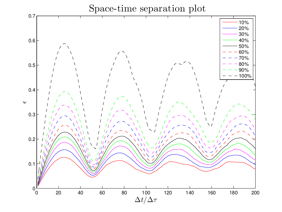
I decided to include in this paper a few words on the widely-used space-time separation plot (STSP), whose visual inspection enables the extraction of an estimate for the temporal interval within which the elements of a given time series are (temporally) correlated. It has been known since a long time (e.g., see Ref. [8] and the references therein) that the temporal correlations affect the evaluation of the correlation sums $C(\epsilon)$, hence the determination of the estimate for the correlation dimension.

Despite the fact that no use of the STSP is called for herein, I will nevertheless concisely describe the method for the sake of completeness, and obtain results from the available data of PG 1159-035. Such information may be useful to those interested in including more of the available data in the dynamically-created database (and therefore need to fix $n_{\rm min}$ in Eq. (6) of Ref. [1]).

For a time-series array comprised of independent elements, the probability $P(d_{ij}\leq\epsilon)$ (i.e., the probability that the distance $d_{ij}$ between two embedding vectors $i$ and $j$ does not exceed a neighbourhood size $\epsilon$) is expected to be only $\epsilon$-dependent; it should not depend on the temporal separation $\Delta t$ between the embedding vectors $i$ and $j$. Therefore, if the percentiles of the $d_{ij}$ distribution are plotted in $2$ dimensions, i.e., as functions of $\epsilon$ (vertical axis) and of $\Delta t$ (horizontal axis), the resulting curves should (in the absence of temporal correlations) be horizontal lines. On the contrary, if temporal correlations are present, a dependence of the percentiles of the $d_{ij}$ distribution on $\Delta t$ is unavoidable. To obtain an estimate for the minimal temporal separation between two elements of a time series, so that these elements be considered uncorrelated, Provenzale and collaborators [9] put forward the following procedure:

• •

  fixation of $\Delta t$ at several values,

• •

  extraction of the $d_{ij}$ distribution for embedding vectors separated by the chosen $\Delta t$ value, and

• •

  determination of the $\epsilon$ values corresponding to certain percentiles of the $d_{ij}$ distribution (e.g., $10\%$, $20\%$, etc.) at the chosen $\Delta t$ value.

The choice of the temporal interval which enables the mitigation/suppression of the effects of the temporal correlations simply reduces to the extraction (from the STSP) of the time above which the percentiles of the $d_{ij}$ distribution are not dependent (at least, in a discernible way) on $\Delta t$.

The STSP, obtained from the available time-series arrays of PG 1159-035, is displayed in Fig. 6. An oscillatory pattern is seen, reflecting the periodicity of the input signal. (Another manifestation of this periodicity is the presence of undulations in the out-of-sample prediction-error arrays $S(k)$.) The STSP of PG 1159-035 is similar to the one obtained by Kantz and Schreiber [8] from the measurements of the flow of a viscous fluid between two coaxial cylinders (Taylor-Couette flow). In my opinion, a reasonable choice of $n_{\rm min}$ would be $2-3$ oscillation periods, i.e., $n_{\rm min}\approx 100-150$ (that is, about the optimal embedding window in this study); Kantz and Schreiber would probably recommend the use of an even larger $n_{\rm min}$ value.

References

- [1] E. Matsinos, ‘Analysis of luminosity measurements of the pre-white dwarf PG 1159-035’, arXiv:1808.05132 [astro-ph.IM].
- [2] http://www.comp-engine.org
- [3] D.E. Winget et al., ‘Asteroseismology of the DOV star PG 1159-035 with the Whole Earth Telectope’, Astrophys. J. 378 (1991) 326–346. DOI: 10.1086/170434
- [4] J.E.S. Costa et al., ‘The pulsation modes of the pre-white dwarf PG 1159-035’, Astron. Astrophys. 477 (2008) 627–640. DOI: 10.1051/0004-6361:20053470
- [5] L. Cao, ‘Practical method for determining the minimum embedding dimension of a scalar time series’, Physica D 110 (1997) 43–50. DOI: 10.1016/S0167-2789(97)00118-8
- [6] P. Grassberger, I. Procaccia, ‘Measuring the strangeness of strange attractors’, Physica D 9 (1983) 189–208. DOI: 10.1016/0167-2789(83)90298-1
- [7] F. James, ‘MINUIT - Function Minimization and Error Analysis’, CERN Program Library Long Writeup D506.
- [8] H. Kantz, T. Schreiber, ‘Nonlinear Time Series Analysis’, Cambridge University Press, 1997; 2nd Edn., Cambridge University Press, 2004. ISBN: 0521821509, 0521529026
- [9] A. Provenzale, L.A. Smith, R. Vio, G. Murante, ‘Distinguishing between low-dimensional dynamics and randomness in measured time series’, Physica D 58 (1992) 31–49. DOI: 10.1016/0167-2789(92)90100-2