Certified Adversarial Robustness
with Additive Noise
Abstract
The existence of adversarial data examples has drawn significant attention in the deep-learning community; such data are seemingly minimally perturbed relative to the original data, but lead to very different outputs from a deep-learning algorithm. Although a significant body of work on developing defensive models has been considered, most such models are heuristic and are often vulnerable to adaptive attacks. Defensive methods that provide theoretical robustness guarantees have been studied intensively, yet most fail to obtain non-trivial robustness when a large-scale model and data are present. To address these limitations, we introduce a framework that is scalable and provides certified bounds on the norm of the input manipulation for constructing adversarial examples. We establish a connection between robustness against adversarial perturbation and additive random noise, and propose a training strategy that can significantly improve the certified bounds. Our evaluation on MNIST, CIFAR-10 and ImageNet suggests that the proposed method is scalable to complicated models and large data sets, while providing competitive robustness to state-of-the-art provable defense methods.
1 Introduction
Although deep neural networks have achieved significant success on a variety of challenging machine learning tasks, including state-of-the-art accuracy on large-scale image classification [1, 2], the discovery of adversarial examples [3] has drawn attention and raised concerns. Adversarial examples are carefully perturbed versions of the original data that successfully fool a classifier. In the image domain, for example, adversarial examples are images that have no visual difference from natural images, but that lead to different classification results [4].
A large body of work has been developed on defensive methods to tackle adversarial examples, yet most remain vulnerable to adaptive attacks [3, 4, 5, 6, 7, 8, 9, 10]. A major drawback of many defensive models is that they are heuristic and fail to obtain a theoretically justified guarantee of robustness. On the other hand, many works have focused on providing provable/certified robustness of deep neural networks [11, 12, 13, 14, 15, 16, 17].
Recently, [18] provided theoretical insight on certified robust prediction, building a connection between differential privacy and model robustness. It was shown that adding properly chosen noise to the classifier will lead to certified robust prediction. Building on ideas in [18], we conduct an analysis of model robustness based on Rényi divergence [19] between the outputs of models for natural and adversarial examples when random noise is added, and show a higher upper bound on the tolerable size of perturbations compared to [18]. In addition, our analysis naturally leads to a connection between adversarial defense and robustness to random noise. Based on this, we introduce a comprehensive framework that incorporates stability training for additive random noise, to improve classification accuracy and hence the certified bound. Our contributions are as follows:
- •
We derive a certified bound for robustness to adversarial attacks, applicable to models with general activation functions and network structures. Specifically, according to [20], the derived bound for perturbation is tight in the binary case.
- •
Using our derived bound, we establish a strong connection between robustness to adversarial perturbations and additive random noise. We propose a new training strategy that accounts for this connection. The new training strategy leads to significant improvement on the certified bounds.
- •
We conduct a comprehensive set of experiments to evaluate both the theoretical and empirical performance of our methods, with results that are competitive with the state of the art.
2 Background and Related Work
Much research has focused on providing provable/certified robustness for neural networks. One line of such studies considers distributionally robust optimization, which aims to provide robustness to changes of the data-generating distribution. For example, [21] study robust optimization over a -divergence ball of a nominal distribution. A robustness with respect to the Wasserstein distance between natural and adversarial distributions was provided in [22]. One limitation of distributional robustness is that the divergence between distributions is rarely used as an empirical measure of strength of adversarial attacks.
Alternatively, studies have attempted to provide a certified bound of minimum distortion. In [11] a certified bound is derived with a small loss in accuracy for robustness to perturbations in two-layer networks. A method based on semi-definite relaxation is proposed in [12] for calculating a certified bound, yet their analysis cannot be applied to networks with more than one hidden layer. A robust optimization procedure is developed in [13] by considering a convex outer approximation of the set of activation functions reachable through a norm-bounded perturbation. Their analysis, however, is still limited to ReLU networks and pure feedforward networks. Algorithms to efficiently compute a certified bound are considered in [14] by utilizing the property of ReLU networks as well. Recently, their idea has been extended by [15] and relaxed to general activation functions. However, both of their analyses only apply to the multi-layer perceptron (MLP), limiting the application of their results.
In general, most analyses for certified bounds rely on the properties of specific activation functions or model structures, and are difficult to scale. Several works aim to generalize their analysis to accommodate flexible model structures and large-scale data. For example, [16] formed an optimization problem to obtain an upper bound via Lagrangian relaxation. They successfully obtained the first non-trivial bound for the CIFAR-10 data set. The analysis of [13] was improved in [17], where it was scaled up to large neural networks with general activation functions, obtaining state-of-the-art results on MNIST and CIFAR-10. Certified robustness is obtained by [18] by analyzing the connection between adversarial robustness and differential privacy. Similar to [16, 17], their certified bound is agnostic to model structure and is scalable, but it is loose and is not comparable to [16, 17]. Our approach maintains all the advantages of [18], and significantly improves the certified bound with more advanced analysis.
The connection between adversarial robustness and robustness to added random noise has been studied in several works. In [23] this connection is established by exploring the curvature of the classifier decision boundary. Later, [24] showed adversarial robustness requires reducing error rates to essentially zero under large additive noise. While most previous works use concentration of measure as their analysis tool, we approach such connection from a different perspective using Rényi divergence [19]; we illustrate the connection to robustness to random noise in a more direct manner. More importantly, our analysis suggests improving robustness to additive Gaussian noise can directly result in the improvement of the certified bound.
3 Preliminaries
3.1 Notation
We consider the task of image classification. Natural images are represented by , where represents the image space, with and denoting the height, width, and number of channels of an image, respectively. An image classifier over classes is considered as a function . We only consider classifiers constructed by deep neural networks (DNNs). To present our framework, we define a stochastic classifier, a function over with output being a multinomial distribution over , i.e., for . One can classify by picking . Note this distribution is different from the one generated from softmax.
3.2 Rényi Divergence
Our theoretical result depends on the Rényi divergence, defined in the following [19].
Definition 1 (Rényi Divergence)
For two probability distributions and over , the Rényi divergence of order is
| (1) |
3.3 Adversarial Examples
Given a classifier for an image , an adversarial example satisfies for some small , and , where is some distance metric, i.e., is close to but yields a different classification result. The distance is often described in terms of an metric, and in most of the literature and metrics are considered. In our development, we focus on the metric but also provide experimental results for . More general definitions of adversarial examples are considered in some works [25], but we only address norm-bounded adversarial examples in this paper.
3.4 Adversarial Defense
Classification models that are robust to adversarial examples are referred to as adversarial defense models. We introduce the most advanced defense models in two categories.
Empirically, the most successful defense model is based on adversarial training [4, 26], that is augmenting adversarial examples during training to help improve model robustness. TRadeoff-inspired Adversarial DEfense via Surrogate-loss minimization (TRADES) [27] is a variety of adversarial training that introduces a regularization term for adversarial examples:
where is the cross-entropy loss. This defense model won 1st place in the NeurIPS 2018 Adversarial Vision Challenge (Robust Model Track) and has shown better performance compared to previous models [26].
On the other hand, the state-of-the-art approach for provable robustness is proposed by [17], where a dual network is considered for computing a bound for adversarial perturbation using linear-programming (LP), as in [13]. They optimize the bound during training to achieve strong provable robustness.
Although empirical robustness and provable robustness are often considered as orthogonal research directions, we propose an approach that provides both. In our experiments, presented in Sec. 6, we show our approach is competitive with both of the aforementioned methods.
4 Certified Robust Classifier
We propose a framework that yields an upper bound on the tolerable size of attacks, enabling certified robustness on a classifier. Intuitively, our approach adds random noise to pixels of adversarial examples before classification, to eliminate the effects of adversarial perturbations.
Our approach is summarized in Algorithm 1. In the following, we develop theory to prove the certified robustness of the proposed algorithm. Our goal is to show that if the classification of in Algorithm 1 is in class , then for any examples such that , the classification of is also in class .
To prove our claim, first recall that a stochastic classifier over has an output corresponding to a multinomial distribution over , with probabilities as . In this context, robustness to an adversarial example generated from means with and , where denotes the probability of an event. In the remainder of this section, we show Algorithm 1 achieves such robustness based on the Rényi divergence, starting with the following lemma.
Lemma 1
Let and be two multinomial distributions over the same index set . If the indices of the largest probabilities do not match on and , that is , then
where and are the largest and the second largest probabilities among the set of all .
To simplify notation, we define as the generalized mean. The right hand side (RHS) of the condition in Lemma 1 then becomes .
Lemma 1 proposes a lower bound of the Rényi divergence for changing the index of the maximum of , i.e., for any distribution , if , the index of the maximum of and must be the same. Based on Lemma 1, we obtain our main theorem on certified robustness as follows, validating our claim.
Theorem 2
Suppose we have , and a potential adversarial example such that . Given a -classifier , let and .
If the following condition is satisfied, with and being the first and second largest probabilities in :
then
The conclusion of Theorem 2 can be extended to the case by replacing Gaussian with Laplacian noise. Specifically, notice the Renyi divergence between two Laplacian distribution and is
Meanwhile, , thus we have the upper bound for the perturbation:
Theorem 3
In the same setting as in Theorem 2, with , let and . If is satisfied, then .
In the rest of this paper, we focus on the norm with Gaussian noise, but most conclusions are also applicable to norm with Laplacian noise. A more comprehensive analysis for norm can be found in [20]. Interestingly, they have proved that the bound is tight in the binary case for norm [20].
With Theorem 2, we can enable certified ( robustness on any classifier by adding i.i.d. Gaussian (Laplacian) noise to pixels of inputs during testing, as done in Algorithm 1. It provides an upper bound for the tolerable size of attacks for a classifier, i.e., as long as the pertubation size is less than the upper bound (the “” part in Theorem 2), any adversarial sample can be classified correctly.
Confidence Interval and Sample Size
In practice we can only estimate and from samples, thus the obtained lower bound is not precise and requires adjustment. Note that () forms a multinomial distribution, and therefore the confidence intervals for and can be estimated using one-sided Clopper-Pearson interval along with Bonferroni correction. We refer to [18] for further details. In all our subsequent experiments, we use the end points (lower for and upper for ) of the confidence intervals for estimating and , and multiply 95% for the corresponding accuracy. Moreover, the estimates for the confidence intervals are more precise when we increase the sample size , but at the cost of extra computational burden. In practice, we find a sample size of is sufficient.
Choice of
The formula of our lower bound indicates a higher standard deviation results in a higher bound. In practice, however, a larger amount of added noise also leads to higher classification error and a larger gap between and , which gives a lower bound. Therefore, the best choice of is not obvious. We will demonstrate the effect of different choices of in the experiments of Sec. 6.
5 Improved Certified Robustness
Based on the property of generalized mean, one can show that the upper bound is larger when the difference between and becomes larger. This is consistent with the intuition that a larger difference between and indicates more confident classification. In other words, more confident and accurate prediction in the presence of additive Gaussian noise, in the sense that is much larger than , leads to better certified robustness. To this end, a connection between robustness to adversarial examples and robustness to added random noise has been established by our analysis.
Such a connection is beneficial, because robustness to additive Gaussian noise is much easier to achieve than robustness to carefully crafted adversarial examples. Consequently, it is natural to consider improving the adversarial robustness of a model by first improving its robustness to added random noise. In the context of Algorithm 1, we aim to improve the robustness of to additive random noise. Note improving robustness to added Gaussian noise as a way of improving adversarial robustness has been proposed by [28] and was later shown ineffective [29]. Our method is different in that it requires added Gaussian noise during the testing phase, and more importantly it is supported theoretically.
There have been notable efforts at developing neural networks that are robust to added random noise [30, 31]; yet, these methods failed to defend against adversarial attacks, as they are not particularly designed for this task. Within our framework, since Algorithm 1 has no constraint on the classifier , which gives the flexibility to modify , we can adapt these methods to improve the accuracy of classification when Gaussian noise is present, hence improving the robustness to adversarial attacks. In this paper, we only discuss stability training, but a much wider scope of literature exists for robustness to added random noise [30, 31].
5.1 Stability Training
The idea of introducing perturbations during training to improve model robustness has been studied widely. In [32] the authors considered perturbing models as a construction of pseudo-ensembles, to improve semi-supervised learning. More recently, [33] used a similar training strategy, named stability training, to improve classification robustness on noisy images.
For any natural image , stability training encourages its perturbed version to yield a similar classification result under a classifier , i.e., is small for some distance measure . Specifically, given a loss function for the original classification task, stability training introduces a regularization term , where controls the strength of the stability term. As we are interested in a classification task, we use cross-entropy as the distance between and , yielding the stability loss , where and are the probabilities generated after softmax. In this paper, we add i.i.d. Gaussian noise to each pixel of to construct , as suggested in [33].
Stability training is in the same spirit as adversarial training, but is only designed to improve the classification accuracy under a Gaussian perturbation. Within our framework, we can apply stability training to , to improve the robustness of Algorithm 1 against adversarial perturbations. We call the resulting defense method Stability Training with Noise (STN).
Adversarial Logit Pairing
Adversarial Logit Pairing (ALP) was proposed in [34]; it adds as the regularizer, with being an adversarial example. Subsequent work has shown ALP fails to obtain adversarial robustness [35]. Our method is different from ALP and any other regularizer-based approach, as the key component in our framework is the added Gaussian noise at the testing phase of Algorithm 1, while stability training is merely a technique for improving the robustness further. We do not claim stability training alone yields adversarial robustness.
6 Experiments
We perform experiments on the MNIST and CIFAR-10 data sets, to evaluate the theoretical and empirical performance of our methods. We subsequently also consider the larger ImageNet dataset. For the MNIST data set, the model architecture follows the models used in [36], which contains two convolutional layers, each containing filters, followed with a fully connected layer of size . For the CIFAR-10 dataset, we use a convolutional neural network with seven convolutional layers along with MaxPooling. In both datasets, image intensities are scaled to , and the size of attacks are also rescaled accordingly. For reference, a distortion of in the scale corresponds to in scale. The source code can be found at https://github.com/Bai-Li/STN-Code.
6.1 Theoretical Bound
With Algorithm 1, we are able to classify a natural image and calculate an upper bound for the tolerable size of attacks for this particular image. Thus, with a given size of the attack , the classification must be robust if . If a natural example is correctly classified and robust for simultaneously, any adversarial examples with will be classified correctly. Therefore, we can determine the proportion of such examples in the test set as a lower bound of accuracy given size .
We plot in Figure 1 different lower bounds for various choices of and , for both MNIST and CIFAR-10. To interpret the results, for example on MNIST, when , Algorithm 1 achieves at least accuracy under any attack whose -norm size is smaller than .

When is fixed, there exists a threshold beyond which the certified lower bound degenerates to zero. The larger the deviation is, the later the degeneration happens. However, larger also leads to a worse bound when is small, as the added noise reduces the accuracy of classification.
As an ablation study, we include the corresponding lower bound without stability training. The improvement due to stability training is significant. In addition, to demonstrate the improvement of the certified bound compared to PixelDP [18], we also include the results for PixelDP. Although PixelDP also has tuning parameters and similar to in our setting, we only include the optimal pair of parameters found by grid search, for simplicity of the plots. One observes the accuracy lower bounds for PixelDP (green) are dominated by our bounds.
We also compare STN with the approach from [17]. Besides training a single robust classifier, [17] also proposed a strategy of training a sequence of robust classifiers as a cascade model which results in better provable robustness, although it reduces the accuracy on natural examples. We compare both to STN in Table 1. Since both methods show a clear trade-off between the certified bound and corresponding robustness accuracy, we include the certified bounds and corresponding accuracy in parenthesis for both models, along with the accuracy on natural examples.
| MNIST | CIFAR-10 | |||
| Model | Robust Accuracy | Natural | Robust Accuracy | Natural |
| [17] (Single) | 1.58 (43.5%) | 88.2% | 36.00 (53.0%) | 61.2% |
| [17] (Cascade) | 1.58 (74.6%) | 81.4% | 36.00 (58.7%) | 68.8% |
| STN | 1.58 (69.0%) | 98.9% | 36.00 (65.6%) | 80.5% |

Our bound is close to the one from [17] on MNIST, and becomes better on CIFAR-10. In addition, since the training objective of [17] is particularly designed for provable robustness and depends on the size of attacks, its accuracy on the natural examples decreases drastically when accommodating stronger attacks. On the other hand, STN is capable of keeping a high accuracy on natural examples while providing strong robustness guarantees.
Certified Robustness on ImageNet
As our framework adds almost no extra computational burden on the training procedure, we are able to compute accuracy lower bounds for ImageNet [37], a large-scale image dataset that contains over 1 million images and 1,000 classes. We compare our bound with PixelDP in Figure 2. Clearly, our bound is higher than the one obtained via PixelDP.
6.2 Empirical Results
We next perform classification and measure the accuracy on real adversarial examples to evaluate the empirical performance of our defense methods. For each pair of attacks and defense models, we generate a robust accuracy vs. perturbation size curve for a comprehensive evaluation. We compare our method to TRADES on MNIST and CIFAR-10. Although we have emphasized the theoretical bound of the defense, the empirical performance is promising as well. More details and results of the experiments, such as for gradient-free attacks, are included in the Appendix.
Avoid Gradient Masking
A defensive model incorporating randomness may make it difficult to apply standard attacks, by causing gradient masking as discussed in [10], thus achieving robustness unfairly. To ensure the robustness of our approach is not due to gradient masking, we use the expectation of the gradient with respect to the randomization when estimating gradients, to ensemble over randomization and eliminate the effect of randomness, as recommended in [10, 38]. In particular, the gradient is estimated as , where ’s are i.i.d. samples from distribution, and is the number of samples. We assume threat models are aware of the value of in Algorithm 1 and use the same value for attacks.
White-box Attacks
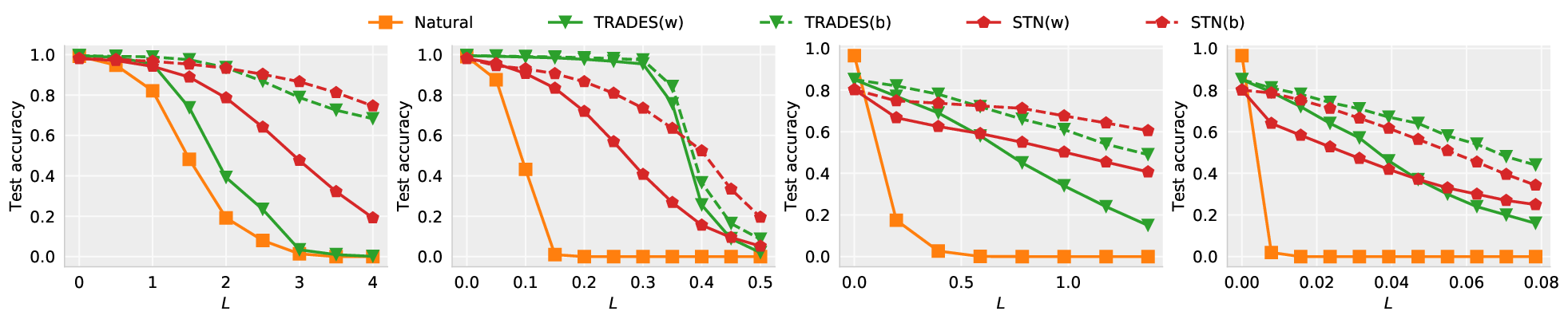
For attacks, we use Projected Gradient Descent (PGD) attacks [26]. It constructs an adversarial example by iteratively updating the natural input along with the sign of its gradient and projecting it into the constrained space, to ensure its a valid input. For attacks, we perform a Carlini & Wagner attack [8], which constructs an adversarial example via solving an optimization problem for minimizing distortion distance and maximizing classification error. We also use technique from [39], that has been shown to be more effective against adversarially trained model, where the gradients are estimated as the average of gradients of multiple randomly perturbed samples. This brings a variant of Carlini & Wagner attack with the same form as the ensemble-over-randomization mentioned above, therefore it is even more fair to use it. The results for white-box attacks are illustrated in Figure 3.

Black-box Attacks
To better understand the behavior of our methods and to further ensure there is no gradient masking, we include results for black-box attacks. After comparison, we realize the adversarial examples generated from Madry’s model [26] result in the strongest black-box attacks for both TRADES and STN. Therefore, we apply the and white-box attacks to Madry’s model and test the resulting adversarial examples on TRADES and STN. The results are reported as the dashlines in Figure 3.
Summary of Results
Overall, STN shows a promising level of robustness, especially regarding -bounded distortions, as anticipated. One observes that STN performs slightly worse than TRADES when the size of attacks is small, and becomes better when the size increases. Intuitively, the added random noise dominantly reduces the accuracy for small attack size and becomes beneficial against stronger attacks. It is worth-noting that Algorithm 1 adds almost no computational burden, as it only requires multiple forward passes, and stability training only requires augmenting randomly perturbed examples. On the other hand, TRADES is extremely time-consuming, due to the iterative construction of adversarial examples.
Choice of
In previous experiments, we use and for MNIST and CIFAR-10, respectively. However, the choice of plays an important role, as shown in Figure 1; therefore, we study in Figure 4 how different values of affect the empirical robust accuracy. The results make it more clear that the noise hurts when small attacks are considered, but helps against large attacks. Ideally, using an adaptive amount of noise, that lets the amount of added noise grow with the size of attacks, could lead to better empirical results, yet it is practically impossible as the size of attacks is unknown beforehand. In addition, we include results for , which is equivalent to a model without additive Gaussian noise. Its vulnerability indicates the essential of our framework is the additive Gaussian noise.
7 Comparison to [40]
Following this work, [40] proposed a tighter bound in norm than the one in section 4. Although they do indeed improve our bound, our work has unique contributions in several ways: We propose stability training to improve the bound and robustness, while they only use Gaussian augmentation. In general, stability training works better than Gaussian augmentation, as shown in Figure 1. Thus, stability training is an important and unique contribution of this paper. We conduct empirical evaluation against real attacks and compare to the state-of-the-art defense method (adversarial training) to show our approach is competitive. [40] only discusses the certified bound and does not provide evaluation against real attacks. The analysis from [40] is difficult to be extended to other norms, because it requires isotropy. On the other hand, ours lead to a tight certified bound by adding Laplacian noise, as discussed in Section 4.
8 Conclusions
We propose an analysis for constructing defensive models with certified robustness. Our analysis leads to a connection between robustness to adversarial attacks and robustness to additive random perturbations. We then propose a new strategy based on stability training for improving the robustness of the defense models. The experimental results show our defense model provides competitive provable robustness and empirical robustness compared to the state-of-the-art models. It especially yields strong robustness when strong attacks are considered.
There is a noticeable gap between the theoretical lower bounds and the empirical accuracy, indicating that the proposed upper bound might not be tight, or the empirical results should be worse for stronger attacks that have not been developed, as has happened to many defense models. We believe each explanation points to a direction for future research.
Acknowledgments
This research was supported in part by DARPA, DOE, NIH, NSF and ONR.
References
- [1] Kaiming He, Xiangyu Zhang, Shaoqing Ren, and Jian Sun. Identity mappings in deep residual networks. In European conference on computer vision, pages 630–645. Springer, 2016.
- [2] Gao Huang, Zhuang Liu, Laurens Van Der Maaten, and Kilian Q Weinberger. Densely connected convolutional networks. In Proceedings of the IEEE conference on computer vision and pattern recognition, pages 4700–4708, 2017.
- [3] Christian Szegedy, Wojciech Zaremba, Ilya Sutskever, Joan Bruna, Dumitru Erhan, Ian Goodfellow, and Rob Fergus. Intriguing properties of neural networks. arXiv preprint arXiv:1312.6199, 2013.
- [4] Ian J Goodfellow, Jonathon Shlens, and Christian Szegedy. Explaining and harnessing adversarial examples. arXiv preprint arXiv:1412.6572, 2014.
- [5] Seyed-Mohsen Moosavi-Dezfooli, Alhussein Fawzi, and Pascal Frossard. Deepfool: a simple and accurate method to fool deep neural networks. In Proceedings of the IEEE Conference on Computer Vision and Pattern Recognition, pages 2574–2582, 2016.
- [6] Nicolas Papernot, Patrick McDaniel, Xi Wu, Somesh Jha, and Ananthram Swami. Distillation as a defense to adversarial perturbations against deep neural networks. In Security and Privacy (SP), 2016 IEEE Symposium on, pages 582–597. IEEE, 2016.
- [7] Alexey Kurakin, Ian Goodfellow, and Samy Bengio. Adversarial machine learning at scale. arXiv preprint arXiv:1611.01236, 2016.
- [8] Nicholas Carlini and David Wagner. Towards evaluating the robustness of neural networks. In Security and Privacy (SP), 2017 IEEE Symposium on, pages 39–57. IEEE, 2017.
- [9] Wieland Brendel, Jonas Rauber, and Matthias Bethge. Decision-based adversarial attacks: Reliable attacks against black-box machine learning models. arXiv preprint arXiv:1712.04248, 2017.
- [10] Anish Athalye, Nicholas Carlini, and David Wagner. Obfuscated gradients give a false sense of security: Circumventing defenses to adversarial examples. arXiv preprint arXiv:1802.00420, 2018.
- [11] Matthias Hein and Maksym Andriushchenko. Formal guarantees on the robustness of a classifier against adversarial manipulation. In Advances in Neural Information Processing Systems, pages 2266–2276, 2017.
- [12] Aditi Raghunathan, Jacob Steinhardt, and Percy Liang. Certified defenses against adversarial examples. arXiv preprint arXiv:1801.09344, 2018.
- [13] J Zico Kolter and Eric Wong. Provable defenses against adversarial examples via the convex outer adversarial polytope. arXiv preprint arXiv:1711.00851, 2017.
- [14] Tsui-Wei Weng, Huan Zhang, Hongge Chen, Zhao Song, Cho-Jui Hsieh, Duane Boning, Inderjit S Dhillon, and Luca Daniel. Towards fast computation of certified robustness for relu networks. arXiv preprint arXiv:1804.09699, 2018.
- [15] Huan Zhang, Tsui-Wei Weng, Pin-Yu Chen, Cho-Jui Hsieh, and Luca Daniel. Efficient neural network robustness certification with general activation functions. In Advances in Neural Information Processing Systems, pages 4944–4953, 2018.
- [16] Krishnamurthy Dvijotham, Robert Stanforth, Sven Gowal, Timothy Mann, and Pushmeet Kohli. A dual approach to scalable verification of deep networks. arXiv preprint arXiv:1803.06567, 2018.
- [17] Eric Wong, Frank Schmidt, Jan Hendrik Metzen, and J Zico Kolter. Scaling provable adversarial defenses. arXiv preprint arXiv:1805.12514, 2018.
- [18] Mathias Lecuyer, Vaggelis Atlidakis, Roxana Geambasu, Daniel Hsu, and Suman Jana. Certified robustness to adversarial examples with differential privacy. arXiv preprint arXiv:1802.03471, 2018.
- [19] Tim Van Erven and Peter Harremos. Rényi divergence and kullback-leibler divergence. IEEE Transactions on Information Theory, 60(7):3797–3820, 2014.
- [20] Anonymous. $\ell_1$ adversarial robustness certificates: a randomized smoothing approach. In Submitted to International Conference on Learning Representations, 2020. under review.
- [21] Hongseok Namkoong and John C Duchi. Variance-based regularization with convex objectives. In Advances in Neural Information Processing Systems, pages 2971–2980, 2017.
- [22] Aman Sinha, Hongseok Namkoong, and John Duchi. Certifiable distributional robustness with principled adversarial training. arXiv preprint arXiv:1710.10571, 2017.
- [23] Alhussein Fawzi, Seyed-Mohsen Moosavi-Dezfooli, and Pascal Frossard. Robustness of classifiers: from adversarial to random noise. In Advances in Neural Information Processing Systems, pages 1632–1640, 2016.
- [24] Nic Ford, Justin Gilmer, Nicolas Carlini, and Dogus Cubuk. Adversarial examples are a natural consequence of test error in noise. arXiv preprint arXiv:1901.10513, 2019.
- [25] T. B. Brown, N. Carlini, C. Zhang, C. Olsson, P. Christiano, and I. Goodfellow. Unrestricted adversarial examples. arXiv preprint arXiv:1809.08352, 2018.
- [26] Aleksander Madry, Aleksandar Makelov, Ludwig Schmidt, Dimitris Tsipras, and Adrian Vladu. Towards deep learning models resistant to adversarial attacks. arXiv preprint arXiv:1706.06083, 2017.
- [27] Hongyang Zhang, Yaodong Yu, Jiantao Jiao, Eric P Xing, Laurent El Ghaoui, and Michael I Jordan. Theoretically principled trade-off between robustness and accuracy. arXiv preprint arXiv:1901.08573, 2019.
- [28] Valentina Zantedeschi, Maria-Irina Nicolae, and Ambrish Rawat. Efficient defenses against adversarial attacks. In Proceedings of the 10th ACM Workshop on Artificial Intelligence and Security, pages 39–49. ACM, 2017.
- [29] Nicholas Carlini and David Wagner. Magnet and" efficient defenses against adversarial attacks" are not robust to adversarial examples. arXiv preprint arXiv:1711.08478, 2017.
- [30] Junyuan Xie, Linli Xu, and Enhong Chen. Image denoising and inpainting with deep neural networks. In Advances in neural information processing systems, pages 341–349, 2012.
- [31] Kai Zhang, Wangmeng Zuo, Yunjin Chen, Deyu Meng, and Lei Zhang. Beyond a gaussian denoiser: Residual learning of deep cnn for image denoising. IEEE Transactions on Image Processing, 26(7):3142–3155, 2017.
- [32] Philip Bachman, Ouais Alsharif, and Doina Precup. Learning with pseudo-ensembles. In Advances in Neural Information Processing Systems, pages 3365–3373, 2014.
- [33] Stephan Zheng, Yang Song, Thomas Leung, and Ian Goodfellow. Improving the robustness of deep neural networks via stability training. In Proceedings of the IEEE Conference on Computer Vision and Pattern Recognition, pages 4480–4488, 2016.
- [34] Harini Kannan, Alexey Kurakin, and Ian Goodfellow. Adversarial logit pairing. arXiv preprint arXiv:1803.06373, 2018.
- [35] Logan Engstrom, Andrew Ilyas, and Anish Athalye. Evaluating and understanding the robustness of adversarial logit pairing. arXiv preprint arXiv:1807.10272, 2018.
- [36] Florian Tramèr, Alexey Kurakin, Nicolas Papernot, Ian Goodfellow, Dan Boneh, and Patrick McDaniel. Ensemble adversarial training: Attacks and defenses. arXiv preprint arXiv:1705.07204, 2017.
- [37] J. Deng, W. Dong, R. Socher, L.-J. Li, K. Li, and L. Fei-Fei. ImageNet: A Large-Scale Hierarchical Image Database. In CVPR09, 2009.
- [38] Nicholas Carlini, Anish Athalye, Nicolas Papernot, Wieland Brendel, Jonas Rauber, Dimitris Tsipras, Ian Goodfellow, and Aleksander Madry. On evaluating adversarial robustness. arXiv preprint arXiv:1902.06705, 2019.
- [39] Bai Li, Changyou Chen, Wenlin Wang, and Lawrence Carin. On norm-agnostic robustness of adversarial training, 2019.
- [40] Jeremy M Cohen, Elan Rosenfeld, and J Zico Kolter. Certified adversarial robustness via randomized smoothing. arXiv preprint arXiv:1902.02918, 2019.
Appendix A Comparison between Bounds
We first use simulation to show our proposed bound is higher than the one from PixelDP [18].
In PixelDP, the upper bound for the size of attacks is indirectly defined: if , where and are two tuning parameters, and the added noise has the distribution , then the classifier is robust to attacks whose size is less than .
As both our and their bound are determined by the models and data only through and , it is sufficient to compare them with simulation for different and as long as , and are satisfied, , and are valid first and second largest output probabilities.
For fixed , and are tuning parameters that affect the result. For a fair comparison, we use a grid search to find and that maximizes their bound.
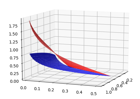
The simulation result in Figure 5 shows our bound is strictly higher than the one from PixelDP. In particular, when and are far apart, which is the most common case in practice, our bound is more than twice as high as theirs.
Appendix B Proof of Lemma 1
Lemma 1 Let and be two multinomial distributions over the same index set . If the indexes of the largest probabilities do not match on and , that is , then
| (2) |
where and are the largest and the second largest probabilities in ’s.
Proof Think of this problem as finding that minimizes such that argmax argmax for fixed . Without loss of generality, assume .
It is equivalent to solving the following problem:
As the logarithm is a monotonically increasing function, we only focus on the quantity part for fixed .
We first show for the that minimizes , it must have . Note here we allow a tie, because we can always let and for some small to satisfy while not changing the Renyi-divergence too much by the continuity of .
If for some , we can define by mutating and , that is , then
which conflicts with the assumption that minimizes . Thus for . Since cannot be the largest, we have .
Then we are able to assume , and the problem can be formulated as
which forms a set of KKT conditions. Using Lagrange multipliers, one can obtain the solution and for , where .
Plug in these quantities, the minimized Renyi-divergence is
Thus, we obtain the lower bound of for argmax argmax.
Appendix C Proof of Theorem 2
A simple result from information theory:
Lemma 4
Given two real-valued vectors and , the Rényi divergence of and is
| (3) |
Theorem 2 Suppose we have , and a potential adversarial example such that . Given a k-classifier , let and .
If the following condition is satisfied, with and being the first and second largest probabilities in ’s:
| (4) |
then
Proof From lemma 4, we know for and such that , with a k-class classification function :
if is a standard Gaussian noise. The first inequality comes from the fact that for any function [19].
Therefore, if we have
| (5) |
It implies
| (6) | ||||
Then from Lemma 1 we know that the index of the maximums of and must be the same, which means they have the same prediction, thus implies robustness.
Appendix D Details and Additional Results of the Experiments
In this section, we explain the details of our implementation of our models and include additional experimental results.
D.1 Gradient-Free methods
We include results for Boundary Attack [9] which is a gradient-free attack method. Boundary attack explores adversarial examples along the decision boundary using a rejection sampling approach. Their construction of adversarial examples do not require information about the gradient of models, thus is an important complement to gradient-based methods.
We test Boundary attacks on MNIST and CIFAR10 and compare them to other attacks considered.

From the plots, one can see Boundary attack is not effective in attacking our models. This is consistent with the observation from [38] that gradient-free method is not effective against randomized models. Nevertheless, we include the results as a sanity check.