from decay and four-flavor lattice QCD
Abstract
Using HISQ MILC ensembles with five different values of the lattice spacing, including four ensembles with physical quark masses, we perform the most precise computation to date of the vector form factor at zero momentum transfer, . This is the first calculation that includes the dominant finite-volume effects, as calculated in chiral perturbation theory at next-to-leading order. Our result for the form factor provides a direct determination of the Cabibbo-Kobayashi-Maskawa matrix element , with a theory error that is, for the first time, at the same level as the experimental error. The uncertainty of the semileptonic determination is now similar to that from leptonic decays and the ratio , which uses as input. Our value of is in tension at the 2– level both with the determinations from leptonic decays and with the unitarity of the CKM matrix. In the test of CKM unitarity in the first row, the current limiting factor is the error in , although a recent determination of the nucleus-independent radiative corrections to superallowed nuclear decays could reduce the uncertainty nearly to that of . Alternative unitarity tests using only kaon decays, for which improvements in the theory and experimental inputs are likely in the next few years, reveal similar tensions and could be further improved by taking correlations between the theory inputs. As part of our analysis, we calculated the correction to due to nonequilibrated topological charge at leading order in chiral perturbation theory, for both the full-QCD and the partially quenched cases. We also obtain the combination of low-energy constants in the chiral effective Lagrangian .
I Introduction
High-precision tests of the unitarity of the Cabibbo-Kobayashi-Maskawa (CKM) matrix, as predicted by the Standard Model (SM), are at the forefront of the current flavor physics program. Any violation of the unitarity of the CKM matrix, which describes flavor-changing interactions, would be evidence of the existence of physics beyond the Standard Model (BSM).
In particular, first-row unitarity, which requires that
| (1) |
vanish, is currently the most precisely tested condition. Even in the absence of deviations, high-precision determinations of the CKM matrix elements involved in the test in Eq. (1) put important constraints on the scale of the allowed new physics [1].
At the current level of precision one can neglect in Eq. (1). Of the other two CKM matrix elements involved, is precisely determined from superallowed nuclear decays [2]. It can also be extracted from measurements of the neutron lifetime [3] and pion decay [4], albeit with much larger errors [5]. Improved experimental measurements of these processes would be interesting because they are theoretically cleaner.
The best determinations of are from kaon decays [6]. The extraction of from semileptonic kaon () decay requires knowledge of the form factor at zero momentum transfer, , which is still the largest source of uncertainty on . On the experimental side, it is expected that the ongoing and forthcoming experiments (NA62, OKA, KLOE-2, LHCb and TREK E36) could reduce the experimental error to within 5 years [7]. Reducing the theoretical error in the vector form factor calculation is therefore a crucial task: it is this task that we take up in this paper.
Determinations of from leptonic kaon and pion decays ( and ), combined with from lattice QCD, currently have somewhat smaller errors than those from . The total error in from leptonic decays is 0.25% [8, 9, 10, 11, 12, 13, 14, 15, 16], while from semileptonic decays it is 0.34% [6]. These leptonic determinations are indirect, however, because they require an external input for , namely Ref. [2]. The direct extraction of from only kaon leptonic decays using as nonperturbative input gives a larger error of 0.46%.11 1 This error is based on the FLAG average for [6], which includes only calculations which do not use , and thus , to set the lattice scale [10, 13, 15].
Currently, the value of obtained from leptonic kaon decay is larger than the value from semileptonic kaon decay [16]. The leptonic decay is mediated by the axial-vector current while the semileptonic decay by the vector current. According to the SM, both approaches should give the same , because the boson current has a structure. Thus, any significant difference should be carefully analyzed.
In addition, if is taken from Ref. [2], the leptonic value of is consistent with unitarity, Eq. (1), but the semileptonic value of leads to a disagreement with unitarity. As we were finishing this work, a paper appeared with a new calculation of the nucleus-independent electroweak radiative corrections involved in the extraction of from superallowed decays with a new approach based on dispersion relations [19]. If this calculation is confirmed, the resulting value of would increase the present tension with unitarity. Investigating the origin of these tensions and performing even more stringent tests is crucial for the internal consistency of the Standard Model. It is thus necessary to reduce the error on both the experimental and the lattice-QCD inputs entering determinations of .
In this paper, we focus on semileptonic kaon decay. The (photon-inclusive) decay rate for can be written [21]
| (2) |
where is the Fermi constant as determined by muon decay, is the universal short-distance electroweak correction [22, 23, 24],22 2 This value of is from Ref. [24]. We use it because it is the value used for the experimental average in Ref. [7]. and is a phase-space integral which depends on the shape of the form factors given in Eq. (4) below. The long-distance electromagnetic corrections are parametrized by . The strong isospin-breaking parameter is defined as a correction with respect to the decay:
| (3) |
so that . The decay rate, , can be obtained by multiplying the right-hand side of Eq. (2) with the Clebsch-Gordan coefficient and replacing , , and with the analogous , , and . The long-distance electromagnetic corrections, which are mode dependent, were calculated to in Ref. [25] and are incorporated into the experimental average for , adding a uncertainty to the experimental errors.
The input needed from lattice QCD in Eq. (2) is the vector form factor at zero momentum transfer, , defined by
| (4) | |||||
where and .
The most precise value for to date is provided by the Fermilab Lattice/MILC calculation in Refs. [26, 27], . More recent lattice-QCD calculations by the RBC/UKQCD () [28] and ETMC () [29] collaborations agree very well with the Fermilab Lattice/MILC central value but with larger errors. Earlier calculations with unphysically heavy pions by the Fermilab Lattice/MILC [30] and RBC/UKQCD [31, 32] collaborations, as well as the more recent JLQCD calculation in Ref. [33], yielded smaller values for , but with larger errors. With the exception of the earliest calculation [32], these results are compatible with the newer ones. For comparison, the average of the relevant experimental input [7], , has a error. This average includes the strong isospin and electromagnetic corrections in Eq. (2) for each decay mode.
In this work we reduce the main sources of uncertainty in our previous calculation of to reach a total error of , obtaining the most precise calculation to date, and matching the current experimental uncertainty, for the first time. The main improvements over our previous calculation [26, 27] are increased statistics in some key ensembles, the addition of a new (smaller) lattice spacing, and the correction of finite-volume effects at next-to-leading order (NLO) in chiral perturbation theory (ChPT). Preliminary results were presented in Refs. [34, 35].
There are other ways to determine . Semileptonic hyperon decays unfortunately lack sufficiently precise knowledge of the SU(3)-breaking corrections, which precludes a competitive determination. A conservative estimate of such effects yields an uncertainty of [36]. Inclusive hadronic decays have, in the past, yielded values of smaller than the semileptonic kaon determination and, thus, were in even more disagreement with unitarity [37]. A more recent analysis [39] uses lattice QCD to compute dimension-larger-than-4 condensates and, more importantly, employs a dispersive technique to obtain the branching fractions. It points to an inclusive- value of compatible with unitarity [39], although it still remains on the low side. An even more promising approach also based on inclusive strange hadronic decay data is presented in Ref. [40]. Its basic ingredients are replacing the operator-product expansion in the relevant sum rules by lattice hadronic vacuum polarization functions and optimizing the weight functions to suppress contributions from the high-energy region, where the experimental data have poor precision. Preliminary results in Ref. [40] are compatible with both semileptonic and leptonic determinations (and thus with unitarity), but have larger errors than either. Because the total errors on in Refs. [38, 39, 40] are dominated by experimental uncertainties, it is expected that these determinations will be significantly improved with new data from the Belle II experiment [41]. Determinations of from exclusive decays, which use the same nonperturbative inputs as the leptonic kaon decay determinations, namely and , are still in tension with unitarity [42], but this could also change with future experimental measurements.
This paper is organized as follows. In Sec. II we describe the methodology of the numerical lattice-QCD simulations and the details of the ensembles, actions, and correlation functions used. Section III shows how, following the ChPT approaches of Refs. [43] and [44], one can correct for leading-order finite-volume effects and for the effects of nonequilibrated topological charge on the ensemble with finest lattice spacing ( fm), respectively. We discuss the joint chiral interpolation and continuum extrapolation of our data to the physical point in Sec. IV. Section V analyzes the statistical and systematic uncertainties. Final results for the form factor , as well as for the relevant low energy constants, are presented in Sec. VI. In Sec. VII, we use our form factor result to extract a value of from kaon semileptonic experimental data and discuss the implications of this value for phenomenology. Finally, we present our conclusions and the prospects for further improvement in Sec. VIII.
II Lattice setup and analysis
The methodology in this work largely follows that of our previous work in Refs. [30, 26, 27]. The approach, pioneered by HPQCD [45], is based on the Ward-Takahashi identity relating the matrix elements of a vector current to that of the corresponding scalar density:
| (5) |
with and the lattice renormalization factors for the vector current and scalar density, respectively, where the scalar density is defined as the product of the scalar current and the quark masses . Working with staggered fermions, and choosing to be the partially conserved, taste singlet, vector current, and to be its divergence, we have . Thus, is a local, taste-singlet density, with the same flavor content as the vector current, . With the above identity and the definition of the form factors in Eq. (4), one can extract the scalar form factor at any value of the momentum transfer by using
| (6) |
In addition, a kinematic constraint requires , so this relation can be employed to calculate from 3-point correlation functions with a scalar insertion. As already discussed in our first work [30], the use of a local scalar density instead of a vector current has two main advantages: avoiding the use of a renormalization factor and avoiding the use of noisier correlation functions with either a nonlocal vector current or external non-Goldstone mesons [45, 46].
II.1 Lattice actions, parameters, and correlation functions
We perform our calculation on the highly-improved staggered quark (HISQ) MILC configurations [47, 48, 49] with sea quarks simulated with the HISQ action [50]. We also employ the HISQ action for the valence quarks. We have already seen in our previous work that the use of the HISQ action greatly reduces discretization effects [26, 27]. The charm-quark and strange-quark masses on the MILC configurations are always tuned to values close to the physical ones, while the light-quark masses vary between and , with the latter approximately the physical value. In this work, we include data generated at five different values of the lattice spacing down to fm, with sea pion masses ranging from to MeV. Table 1 lists the key parameters of the ensembles analyzed here and the correlation functions calculated on them. The ensembles include four with physical quark masses and fm. Ensembles that are new since our analysis in Refs. [26, 27] are marked with a dagger in the last column; those where we have increased the statistics are marked with an asterisk. Table 1 also lists the pseudoscalar-taste (physical) pion mass and the root-mean-squared pion mass for each ensemble. The difference is a measure of the dominant discretization effects, which arise from taste-changing interactions. As expected, they decrease rapidly as the lattice spacing is reduced. The data included in this analysis are graphically depicted in Fig. 1.
| 0.15 | 0.035 | 3.2 | 1000 | 4 | 12,13,15,16,17,18 | 0.0647 | 0.06905 | 130 | 314 | ||
| 0.12 | 0.2 | 4.5 | 1053 | 8 | 15,18,20,21,22 | 0.0509 | 0.0535 | 299 | 364 | ||
| 0.1 | 3.2 | 1020 | 8 | 15,18,20,21,22 | 0.0507 | 0.053 | 221 | 303 | |||
| 0.1 | 4.3 | 993 | 4 | 15,18,20,21,22 | 0.0507 | 0.053 | 216 | 299 | |||
| 0.1 | 5.4 | 1029 | 8 | 15,18,20,21,22 | 0.0507 | 0.053 | 214 | 298 | * | ||
| 0.035 | 3.9 | 945 | 8 | 15,18,20,21,22 | 0.0507 | 0.0531 | 133 | 246 | |||
| 0.09 | 0.2 | 4.5 | 773 | 4 | 23,27,32,33,34 | 0.037 | 0.038 | 301 | 323 | ||
| 0.1 | 4.7 | 853 | 4 | 23,27,32,33,34 | 0.0363 | 0.038 | 215 | 221 | |||
| 0.035 | 3.7 | 950 | 8 | 23,27,32,33,34 | 0.0363 | 0.0363 | 130 | 176 | * | ||
| 0.06 | 0.2 | 4.5 | 1000 | 8 | 34,41,48,49,50 | 0.024 | 0.024 | 304 | 308 | * | |
| 0.035 | 3.7 | 692 | 6 | 31,39,40,48,49 | 0.022 | 0.022 | 135 | 144 | |||
| 0.042 | 0.2 | 4.3 | 432 | 12 | 40,52,53,64,65 | 0.0158 | 0.0158 | 294 | 296 |
The structure of the three-point function with a scalar insertion that we generate to access the matrix element in Eq. (6) is the same as in our previous work [30, 26, 27]. We generate light quarks at a time slice and extended strange propagators at a fixed distance from the source. For each configuration we have time sources placed at , where is the temporal length of the lattice. The time varies randomly from configuration to configuration in an interval to reduce autocorrelations. Roughly following Ref. [51] we use random-wall sources at the pion source time . On that spatial time-slice, we choose four stochastic color-vector fields from a Gaussian distribution, with support on all three colors, and compute light-quark propagators from each of the four sources. Between the source and the kaon sink at time , we contract the extended strange propagator with a light propagator to form the scalar density. We then study the dependence to isolate the desired matrix element.
The light-quark masses are always the same in the sea and valence sectors, while the sea and valence strange-quark masses are slightly different in some of the ensembles33 3 At the time the analysis began, the physical value of on those ensembles had been determined more accurately than when the ensembles were generated. We used the more accurate values for the valence strange-quark mass to be closer to the physical point.; see Table 1. Table 1 also lists the number of configurations and time sources on each ensemble. We compute three-point functions as described above for 5 or 6 different values of the source-sink separation , listed in Table 1, which correspond to approximately the same physical distances across ensembles. We include both even and odd values of to disentangle the effects from oscillating states in the correlation functions.
We simulate directly at zero momentum transfer, , by tuning the external momentum of the pion using partially twisted boundary conditions. In particular, we tune
| (7) |
with the twist angle of the daughter propagator going from the pion to the current. The rest of the propagators are generated with periodic boundary conditions, the same as in the sea sector. We always have diagonal twist angles, , which turn out to give smaller finite-volume effects than twisting in only one direction [43]. The values of for each ensemble, as well as the corresponding momentum of the pion, are given in Table 2.
For each ensemble, we generate zero-momentum two-point and correlation functions and two-point correlation functions with external momentum given by the twist angle , defined in Eq. (7). These correlators are given by
| (8) |
where the interpolating operator creates a meson at time with momentum . The random wall sources automatically implement the sum over . We also generate three-point correlation functions with the kaon at rest:
| (9) |
where the pion recoil momentum is either equal to zero or to the values listed in Table 2. The scalar density is a local taste-singlet.
| 0.15 | 0.035 | 3.2 | 1.80966 | 0.17766 |
| 0.12 | 0.2 | 4.5 | 0.84749 | 0.11094 |
| 0.1 | 3.2 | 0.98192 | 0.12853 | |
| 0.1 | 4.3 | 1.30923 | 0.12853 | |
| 0.1 | 5.4 | 1.63653 | 0.12853 | |
| 0.035 | 3.9 | 2.16464 | 0.14168 | |
| 0.09 | 0.2 | 4.5 | 0.82675 | 0.08117 |
| 0.1 | 4.7 | 1.45024 | 0.09492 | |
| 0.035 | 3.7 | 2.08413 | 0.10230 | |
| 0.06 | 0.2 | 4.5 | 0.81673 | 0.05345 |
| 0.035 | 3.7 | 2.01756 | 0.06602 | |
| 0.042 | 0.2 | 4.3 | 0.78006 | 0.03829 |
II.2 Fit methods and statistical analysis
The fitting strategy we follow to extract the physical quantities from our correlation functions has already been discussed in Refs. [30, 54]. We fit the two-point correlation functions for a pseudoscalar meson to the expression
| (10) |
using Bayesian techniques. In Eq. (10), is the temporal size of the lattice. The oscillating terms with do not appear for a zero-momentum . We fit the three-point correlation functions to
| (11) | |||||
where the pion and kaon energies and amplitudes, , , and , are the same as those appearing in the two-point fit functions.
We first fit the two-point functions one by one on each ensemble and check the stability of the ground state masses/energies and amplitudes under the choice of fitting range, , and the number of exponentials included in the fit function [ in Eq. (10)]. We always include the same number of regular and oscillating states in those fits, i.e., . To evaluate the relative quality of the fits we use the and the value defined in Ref. [53], a quality of fit statistic adapted for fits with Bayesian priors that is similar to the standard value [3]. By construction, with larger values indicating greater compatibility between the data and fit function given the prior constraints —see Ref. [53] for details and explicit formulas. In particular, we disregard any fit with . We also disregard fits with , since those low are generally an indication of a bad identification of the ground state and the corresponding fits tend to be unstable with the variation of , number of exponentials, and/or bootstrap resampling.
We observe that for most of the choices of time range and for all ensembles, fits stabilize when including 2+2 or 3+3 states. From that parameter-scanning procedure, we select an optimal set of fit parameters for the two-point functions, with a common for all the functions on the same ensemble. Fixing , the chosen is the smallest value for which the ground state parameters for all relevant two-point functions reach a plateau and, in addition, for which the fit results (central values, errors, and quality) are stable under variations of the number of exponentials and bootstrap resampling. For a fixed , is chosen, in general, as the value for which fit results are insensitive to the addition of late-time data for which statistical errors are larger.
We then use those ranges to perform a fully correlated combined Bayesian fit including the two- and three-point functions needed to extract : two-point correlation functions with and without momentum, two-point correlation functions without momentum, and three-point correlation functions with , where is the number of source-sink separations included in the combined fit. In general, we include three-point functions only at or 4 different values of out of the 5 or 6, for which we have data. However, the values included in the combined fits generally cover most of the available range, corresponding to a physical range of fm. This allows us to resolve excited states while at the same time including data with good ground state contributions. We find that the resulting fits are stable under variations of time range, number of exponentials, and bootstrap resampling. We also find that adding more values does not improve the quality (error and stability) of the fits. Table 3 lists our parameter choices for the combined three-point function fits.
In general, we use three-point data in the combined fits with , where is the value optimized for the two-point functions. However, on some ensembles, especially the largest ones, we need to either shorten the three-point fit range or thin the three-point data in order to obtain an acceptable fit, as measured by the and value. A comparison of fit results to data for the fm ensemble with physical quark masses, one of the most relevant in our analysis, is given in Fig. 2. This is a typical case, the comparisons of the fits and data on the other ensembles are similar. The figure plots the rescaled three-point functions, in which the time-dependent contributions of the kaon and pion ground states are removed:
| (12) |
In the absence of excited state contributions would be time independent. Figure 2 shows the comparison of the rescaled correlation functions included in the fit (filled green points) with the results from the fit (open orange circles). We see that the exhibit plateaus with a mild oscillation that is more pronounced for the smaller value, but which can be accounted for almost entirely by the first oscillating state included in the fit. The agreement between data and the fit is excellent, especially for the time ranges included in the fit, marked by the orange lines. For times closer to the source or the sink, the large errors on the orange points indicate a substantial contribution from the excited states included in the fit that the data cannot constrain accurately. Nevertheless, the falloff of the correlators is well described by the fit functions.
From the combined fits, we extract the scalar form factor at zero momentum transfer via
| (13) |
where is the ground state three-point parameter in Eq. (11), the meson masses and energies are the values extracted from the combined fits and and are the valence strange and light-quark masses simulated.
We check the stability of the combined fit results under the variation of fit ranges, number of states, and number and values of source-sink separations included, and choose a preferred fit for each ensemble so the shift on the central value with those variations is well under the statistical error, and the error is also stable. Examples of these stability studies are shown in Fig. 3. On a few ensembles, the stability tests lead to slight adjustments of our chosen value of , from the determined in the two-point only fits discussed above. Our final choices of correspond to very similar physical distances, approximately 0.6–0.7 fm, on each ensemble. The number of exponentials is always chosen to be 3+3, since also for these combined fits adding more exponentials does not change the fit results and also does not improve fit stability. The parameter values used in the preferred combined fits are listed in Table 3.
We study the effect of autocorrelations by blocking the data by increasing numbers of successive configurations and redoing the analysis. We do not see evidence of significant autocorrelations on all ensembles, but for those where we do see significant changes in central value and error, stability is reached with a block size of four. For ensembles where we observe significant changes in central value and error for the form factor with blocking, those effects stabilize when blocking by four. An example for the ensemble with fm and physical quark masses is given in Fig. 4. Similar results are obtained for the other ensembles. An alternate estimate of autocorrelation effects can be obtained by calculating the integrated autocorrelation time. We find that the integrated autocorrelation times in the two-point correlation functions included in our analysis are all smaller than 1.4, suggesting that a reasonable block size would be 3 or less. We thus choose to account for autocorrelation effects and block the data in all ensembles by four. In a another test, we construct the covariance matrix from the correlation matrix obtained with the unblocked data together with the variances obtained from the blocked data [49]. Using the same fit setup and parameter choices as before, we find results that are essentially the same as those obtained with our preferred fit method.
| 0.15 | 0.035 | 3.2 | 12,16,17 | 4 | 0.9744(24) | |
|---|---|---|---|---|---|---|
| 0.12 | 0.2 | 4.5 | 15,21,22 | 5 | 0.9874(24) | |
| 0.1 | 3.2 | 15,18,21 | 4 | 0.9830(31) | ||
| 0.1 | 4.3 | 15,18,21 | 4 | 0.9808(22) | ||
| 0.1 | 5.4 | 15,18,21 | 4 | 0.9809(17) | ||
| 0.035 | 3.9 | 18,21,22 | 6 | 0.9707(18) | ||
| 0.09 | 0.2 | 4.5 | 27,32,33 | 3 | 0.9868(18) | |
| 0.1 | 4.7 | 23,27,32 | 6 | 0.9807(22) | ||
| 0.035 | 3.7 | 23,27,32 | 8 | 0.9709(27) | ||
| 0.06 | 0.2 | 4.5 | 34,41,49,50 | 8 | 0.9862(16) | |
| 0.035 | 3.7 | 31,40,49 | 10 | 0.9697(33) | ||
| 0.042 | 0.2 | 4.3 | 40,52,53 | 12 | 0.9856(37) | 0.0010 |
In Table 3 and Fig. 5, we show the raw results for the vector form factor at zero momentum transfer from the combined fits described above. The statistical errors shown in the table and the figure as a function of come from 500 bootstrap resamples and range from to . The fully correlated covariance matrix is recalculated on each bootstrap resample. In the figure, one can see that for a fixed value of the light-quark mass, , the points with different shapes, which correspond to different values of the lattice spacing, lie on top of each other, with the exception of the data point for the fm ensemble with physical quark masses (in the leftmost cluster of points). This is the only ensemble where we observe statistically significant discretization effects.
III Form-factor corrections
Before performing the chiral-continuum fit, we correct the form factor results listed in Table 3 and shown in Fig. 5 for the leading-order finite-volume effects and the nonequilibrated topological charge in our finest ensemble. These corrections are described in the following two subsections.
III.1 Finite volume
In this work we use NLO ChPT to correct our form factor results for finite-volume effects, whereas in our previous calculation [26, 27] we simply estimated the associated systematic error from a comparison of the lattice data at two different spatial volumes, with other parameters held fixed. The partially twisted boundary conditions used in our calculation introduce several complications in the analysis. In particular, an extra form factor is required to parametrize the weak-current matrix element in finite volume:
| (14) |
The three form factors depend on the choice of twisting angles, as well as the value of .
We apply the one-loop formulas in Ref. [43] in the staggered partially-twisted partially-quenched case to all ensembles included in our calculation for the choices of twist angles in Table 3. Because we are calculating the vector form factor at zero momentum transfer via the relation in Eq. (6), and the quantity we obtain at finite volume on the lattice is , the FV correction to our results is given by
| (15) | |||||
where the meson masses in the denominators are the ones from the simulations, and quantities that are second order in the finite-volume corrections have been neglected. In Eq. (15), the FV correction for a given quantity , , is defined as . Notice that, since we extract the meson masses from correlation functions where all the propagators have zero momentum, the FV corrections to the meson masses should be calculated from the formulas in Ref. [43] with zero twisting angles.
The resulting FV corrections are listed in the last column of Table 3. We find that they are on all ensembles. Some of the values for are particularly small due to the cancellation between the two contributions in Eq. (15). We subtract the from the finite-volume (listed in the next-to-last column in Table 3) before performing the chiral-continuum fit discussed in Sec. IV.
III.2 Nonequilibrated topological charge
The HISQ MILC simulations with smallest lattice spacings have reached a regime where the distribution of the topological charge is not properly sampled [55, 44], which affects the physical observables calculated on those ensembles. The issue is relevant here for the ensemble with the finest lattice spacing, fm. On the other hand, the topological charge is reasonably well equilibrated on the other ensembles, which have fm.
In order to correct for this systematic effect, one can use ChPT to study the -dependence of a given observable [56, 57, 44]. The recent ChPT study in Ref. [44] has already been applied to the calculation of heavy-light meson decay constants and masses in Refs. [49, 58]. Here, we extend the analysis of Ref. [44] to .
The three-point correlation functions relevant for this study, as well as any meson mass calculated in a finite volume and at fixed , satisfy [56, 57]
| (16) |
where on the right-hand side is the infinite-volume value of the quantity of interest averaged over , is its second derivative with respect to the vacuum angle , evaluated at , and is the infinite-volume topological susceptibility. Knowing the dependence on or, equivalently, on , one can calculate the appropriate correction to to account for the difference between the correct and the simulation .
With Eq. (16), we follow Ref. [44] to calculate the correction as
| (17) |
where is the simulation value.
Although we extract from the scalar-density matrix element in Eq. (6) it is simpler to first calculate the dependence of the vector-current matrix element directly. In ChPT, the vector current with the relevant flavor is
| (18) |
where is the SU(3) chiral matrix. In the presence of , and for the and full QCD case (the case relevant for this work), the ChPT Lagrangian is
| (19) |
where is the chiral-limit value of the meson decay constant, and the low energy constant that relates meson and quark masses at leading order (LO)—see Eq. (37). Here , with the usual quark mass matrix in the absence of .
When , gets the vacuum expectation value
The parameter encodes the dependence on , with . The relation between and is obtained by minimizing the potential energy term in the Lagrangian, which gives the condition
| (24) |
For the expansion of the relevant observables, one needs , the first derivative of with respect to evaluated at . Equation (24) implies [44]
| (25) |
One may expand around its vacuum expectation value via
| (26) |
with the matrix of meson fields. With this result substituted into Eq. (18), at tree level there are two possible diagrams, shown in Fig. 6, that may contribute to the matrix element . The strong three-point vertex in the right-hand diagram is forbidden by parity when , but here comes from the mass term in Eq. (19), which violates parity symmetry unless one also takes (which is called “extended parity”). The weak vertex in the right-hand diagram generates a factor of , implying that that diagram contributes only to the form factor . From the left-hand diagram, one finds
| (27) |
Finally, from Eq. (25), the result needed to adjust the form factor via Eq. (17) is
| (28) |
Because we actually use Eq. (6) to calculate , it is important to check that we can reproduce Eq. (28) by calculating the matrix element of the scalar density that appears in the Ward identity at ,
| (29) |
with , and the appropriate flavor matrix to select the current. Note that it is no longer convenient to take out a factor of from , as we do for in Eq. (6), because the quark masses now carry factors of . In ChPT,
| (30) |
Evaluating the diagrams in Fig. 6, we find
| (31) | |||||
where the contributions in the first and second lines come from the propagator and vertex diagrams in Fig. 6, respectively.
The Ward identity in Eq. (29) is then satisfied trivially at LO for . For , we may calculate from Eq. (29) using Eq. (25), the fact that (which follows from extended parity), and the second derivatives
| (32) |
from [44]. After some algebra, we find that the result agrees with Eq. (28), as expected. We have also checked analytically that the Ward identity holds for arbitrary and .
Following the procedure in Ref. [44] for the partially quenched case, we may generalize Eq. (28) to
| (33) |
where and are the active valence quarks (the valence up and strange for ), and and are the light and strange sea quark masses. In deriving Eq. (33), we have set the spectator quark mass (the quark mass for ) equal to the light sea mass ; in other words, the spectator quark is unitary, not partially quenched. This has allowed us to avoid analyzing the case of three partially quenched quarks, which was not treated in Ref. [44]. Since the mass of the spectator quark does not affect to LO, we believe Eq. (33) will remain valid even when the spectator quark is partially quenched. As expected, Eq. (33) reduces to Eq. (28) when and .
As discussed at the beginning of this section, the correction is only needed on the finest ensemble included in this analysis, with fm. We calculate the correction of Eq. (17) using Eq. (28), the value of the average of the topological charge measured on that ensemble, [44], and the correct as estimated by the LO ChPT expression for the topological susceptibility [73, 74]
| (34) |
where the singlet meson sea masses are defined in Eq. (37), below. The resulting correction is subtracted from the value listed in the last row of Table 3 before performing the chiral-continuum fit.
IV Chiral-continuum interpolation/extrapolation
We follow a methodology very similar to that in our previous analyses [26, 27] in order to combine our simulation data into physical results in the continuum limit and with the correct quark/meson masses. Here we summarize the main ingredients and then discuss in more detail the new features added in order to accurately account for finite-volume and isospin-breaking corrections. Accounting for these effects turns out to be essential, given the improvements in the simulation data.
Our methodology is developed in the framework of chiral perturbation theory (ChPT), which allows us to incorporate effects due to mass dependence, discretization, finite volume, and isospin breaking in a systematic way. In particular, in the isospin limit, we can write as a chiral expansion
| (35) |
where the functions are chiral corrections of . The Ademollo-Gatto (AG) theorem [59] ensures that the vector form factor goes to 1 in the limit , and that corrections to this limit are second order. That means that the functions are proportional to or, equivalently, . The theorem thus implies that, in the continuum, the (one-loop) contribution, , is completely fixed in terms of experimental quantities: the decay constant and meson masses.
The specific fit function we employ for the extrapolation to the continuum and interpolation to the physical quark masses is the same as in Ref. [26]. It consists of a NLO partially quenched staggered ChPT (PQSChPT) expression [60] , plus NNLO continuum ChPT terms [61] , plus extra analytic terms to parametrize higher-order discretization and chiral effects. Schematically, it can be written
| (36) |
where the functions and account for higher-order discretization effects, and the function includes analytical terms that parametrize higher-order chiral effects. We have taken the pure counterterm contribution at two loops out of and written it separately. This contribution corresponds to the term proportional to , which is given by the combination of low energy constants (LECs) . The LEC can be extracted from global fits or from lattice-QCD calculations of light-light quantities, but the LECs and [62, 63] are not known. (Only model-based estimates and imprecise global fit values exist.) We therefore take as a constrained fit parameter. All dimensionful quantities entering in the fit function in Eq. (36) are converted into units by using the values of in Table 4.
| (fm) | 0.15 | 0.12 | 0.09 | 0.06 | 0.042 | continuum |
|---|---|---|---|---|---|---|
| fm | ||||||
| MeV | ||||||
| 1.2163 | ||||||
| 2.0565 | 1.6994 | 1.2820 | 0.8873 | 0.6986 | ||
| 2.090(6) | 2.608(4) | 3.588(7) | 5.442(10) | 7.143(24) | ||
| 0 | 0 | 0 | 0 | 0 | ||
| 0.301197 | 0.167563 | 0.052723 | 0.009542 | 0.004794 | ||
| 0.204127 | 0.103326 | 0.034894 | 0.006974 | 0.003504 | ||
| 0.106046 | 0.053983 | 0.018187 | 0.003588 | 0.001803 | ||
| 0.399862 | 0.209269 | 0.066393 | 0.012493 | 0.006276 | ||
Since our simulations are performed in the isospin limit, , and are evaluated for degenerate up and down quarks. The explicit NLO PQSChPT function can be found in Ref. [60]. It incorporates the dominant discretization effects coming from the taste-symmetry breaking of staggered fermions. The function depends on the HISQ taste splittings through the sea meson masses
| (37) |
with sea quark masses, the slope to be determined by fits of the ChPT expressions to experimentally measured meson masses, and labeling the meson taste. Values of for each ensemble are given in Table 4. The function also depends on the taste-violating hairpin parameters, and , which come from ChPT disconnected diagrams. We fix the taste splittings in the fit function to their values in Table 4 since they are precisely enough known that the corresponding errors do not affect our results significantly. The values are from Ref. [48], as well as unpublished updates with better statistics and the inclusion of new ensembles not previously analyzed. The uncertainty in the hairpin parameters is, however, quite large. We therefore treat them as constrained fit parameters with central values and widths equal to those in Table 5, determined from fits to light-light meson quantities [68]. Their uncertainty is thus propagated to the final fit errors.
| Fit parameters | Gaussian priors | ChPT fit |
| (central value width) | posteriors | |
For some of the meson masses that appear in there are no experimental measurements or lattice results, as for example, for or for the sea-valence meson masses involving strange quarks. Because we use values given by NLO ChPT for these masses, our function has some dependence on the corresponding LECs . This is the best approximation we have, and we find that different implementations of higher-order corrections result in changes to the central values that are significantly smaller than the statistical errors.
The continuum NNLO ChPT function also depends on the LECs. We take most of them as constrained fit parameters with prior central values equal to the posteriors obtained in the global fit BE14 in Ref. [67]. We take as an input parameter the combination instead of because the fit is more sensitive to that combination and because is fixed in fit BE14. The prior widths are set to twice the errors in Ref. [67]. The chiral scale, at which the LECs and chiral logarithms in the ChPT expression of Eq. (36) are evaluated, is set equal to the mass of the meson, i.e., . The LECs from Ref. [67], used as priors here, agree within errors with (but are more precise than) the only realistic lattice calculations available at the moment: the MILC [13] and the HPQCD [12] calculations. The prior central values and widths used in our chiral-continuum fit to Eq. (36) are listed in Table 5.
The LECs and appear only in the isospin corrections and in the NLO expressions for some of the meson masses in and . Their effect on and in the isospin limit is, however, negligibly small, and their main impact is via the isospin-breaking corrections, which are added after performing the chiral-continuum fit (see Sec.V.6). We choose then to take and as fixed parameters in the chiral-continuum fit and include their uncertainties in the total error as described in Sec. V.2.
Once the taste-violating discretization errors for staggered fermions are removed through the explicit dependence on of , the dominant discretization errors at in ChPT are and . Since we are forced to use continuum ChPT at , the discretization errors there are and . We take these errors into account through the functions and in Eq. (36):
| (38a) | |||
| (38b) | |||
where the are fit parameters, is the average taste splitting, and is a proxy for . Table 5 lists the priors employed for the s. The terms proportional to and are generic terms parametrizing discretization effects of and , respectively, obeying the AG theorem. We include the terms proportional to and to account for and violations of the AG theorem at finite lattice spacing arising from symmetry-breaking discretization effects in the form factor decomposition, Eq. (4), and in the continuum dispersion relation. We find that adding an term instead of the one proportional to yields fit results that are nearly identical.
As in Refs. [26, 27], we also add generic analytical terms corresponding to higher orders in the chiral expansion until the error of the chiral-continuum fit saturates, i.e., until the central value, the error and the (and ) value do not change appreciably. That happens at N4LO []—see Sec. V. The function in Eq. (36), which collects these effects, therefore takes the form
| (39) |
The terms proportional to and are and , respectively. The are constrained fit parameters; the priors for them can be found in Table 5. Further discussion of the fit function, priors used in the Bayesian approach, and tests performed can be found in Refs. [26, 27].
IV.1 Fit results
We fit our finite-volume corrected form factor data to the functional form in Eq. (36) with the functions and given in Eqs. (38) and (39), respectively. All the results listed in Table 3 are included in our central-value fit, except for the ensemble with fm and , which we use only to check finite-volume effects. We then extrapolate to the continuum limit and interpolate to the pure-QCD meson masses, i.e., with electromagnetic effects removed, using the parameters determined from the fit described above together with the continuum isospin-breaking NNLO ChPT expressions in Ref. [69], plus the N3LO and the N4LO chiral terms in Eq. (39), which do not vanish in the continuum limit. We take the pure-QCD masses from Ref. [49]:44 4 The QCD mass is just the experimental one, and the QCD mass includes the estimate of the small isospin-breaking correction, which comes from Ref. [72]. , , , . For the case we find
| (40) |
where the error is from the fit only, and does not yet include all systematic effects. The statistical error is estimated by fitting to a set of 500 bootstrap samples for each ensemble. On each of those fits, we randomly change the central values of all the priors sampling over Gaussian distributions, keeping the same widths as in Table 5. The plot in Fig. 7 shows, as a function of the light-quark mass, the central interpolation curve as well as its error band in the continuum and with the strange-quark mass adjusted to its physical value. In order to make the comparison to data clearer, the curve in Fig. 7 does not include any strong isospin-breaking effects, i.e., . The point at the physical masses (yellow star) in Fig. 7, however, is our central result in Eq. (40), which includes strong isospin-breaking effects at NNLO.
The result in Eq. (40) includes isospin corrections up to NNLO—see Sec. V.6 for more details. For decays, isospin corrections enter only at NLO () and beyond, and are small, . It also includes corrections for the leading-order finite-volume effects as described in Sec. III.1.
The second column in Table 5 shows the posteriors for the fit parameters of the chiral-continuum fit that leads to the result in Eq. (40). We cannot determine the coefficients accurately since there is very little dependence in our results. In fact, if we remove the fm point we could fit our data without including discretization effects at all. Our lattice data also provide little constraint on the individual values of the LECs. As seen in Table 5, the posterior fit values of the are generally the same as the priors.
V Systematic error analysis
The error in Eq. (40) includes statistical, chiral-extrapolation, and discretization errors, as well as the uncertainties associated with the inputs that are treated as constrained fit parameters: LECs (except ) and taste-violating hairpin parameters. The uncertainties of the data and constrained input parameters are propagated through the fit via 500 bootstrap resamples.
In this section, we further study these sources of uncertainty, perform tests of the stability of our preferred fit strategies, and estimate the other sources of systematic error entering in our calculation of : uncertainty in the inputs, scale error, partial-quenching effects, higher-order finite-volume effects, isospin-breaking corrections, and the effects of nonequilibrated topological charge.
V.1 Fit function, discretization error and chiral interpolation
Because we have data at the physical light-quark masses, the chiral fit is an interpolation, and is largely independent of the precise form of the fit function and the values of the ChPT parameters. We have performed a number of tests to check this stability under variations in the fit function and to estimate the effect of higher-order terms in the chiral and Symanzik expansions. Figure 8 shows the tests performed and discussed in this subsection, together with the results from additional fits discussed in the following subsections, which we use to estimate several systematic uncertainties.
First of all, in order to be sure that effects due to higher-order terms in the chiral expansion are properly included in the Bayesian analysis that leads to the fit error shown in Eq. (40), we need to check that this error stabilizes as we add higher-order chiral terms. The point labeled NNLO in Fig. 8 includes only terms up to NNLO, i.e., without the function in Eq. (36). Only minimal changes in the central value and errors are produced by the addition of the N3LO term from Eqs. (39) and (36). The difference between this and the base fit is the N4LO term , and we see that it has a negligibly small effect.
Different values of the decay constant used in the two-loop (NNLO) term are equivalent up to omitted higher-order terms, and therefore should have a negligible effect on our analysis. In contrast, the decay constant at one loop has to be set equal to the physical pion decay constant, , in order to be consistent with the particular expression chosen for . In the base fit, we use as the chiral expansion parameter in . We check that other possible choices, such as MeV [16] (labeled “ vs. at two loops” in Fig. 8) and an estimate of the decay constant in the chiral limit, MeV [13], shift the central value in Eq. (40) by less than 0.06%, well under the statistical error.
As another test of the ChPT fit and errors, we replace the continuum two-loop ChPT expression in Eq. (36), , by an analytic function, and consecutively add N3LO and N4LO analytic terms—see results labeled “NNLO analyt.,” “N3LO analyt.,” and “N4LO analyt.,” respectively, in Fig. 8. All the results agree very well with our base fit within statistics, being nearly identical once the N3LO analytic term is included.
The three results labeled “no analyt. ” (which corresponds to a fit without including and in the fit function), “”, and “” in Fig. 8 represent a check that the discretization errors are properly included in the fit error of Eq. (40). Once we include the term of order (proportional to ) in Eq. (38), which is required to get a fit of similar quality to our base fit —see Fig. 8, the central value and errors barely change with the addition of corrections (the result labeled “”). Adding the two remaining discretization terms in and , which returns us to the base fit, makes no noticeable difference. The rapid stabilization of the fit reflects the tiny lattice-spacing dependence of our data.
Of all the data in Fig. 5, only the point at fm shows what appear to be significant discretization effects. Dropping that data point has the effect of increasing the errors (see result labeled “no fm”), since the other ensembles provide very little constraint of the analytical fit parameters. In fact, after dropping that point, we can fit our remaining data with a continuum fit function, although we see from Fig. 8 (result labeled “continuum, no fm”) that the result is larger than our central result by about two standard deviations, measured in terms of the fit errors, and the quality of the fit significantly drops. Adding analytical discretization corrections via the functions and to the continuum fit function allows us to fit all our data, giving a result that is consistent with the base fit and with a similar value (see result labeled “continuum + analyt. ”), although with a larger error.
In contrast to the noticeable effect of the coarsest ensemble on the total error, the effect of our finest lattice spacing, fm, on the central value and the error is very small since statistics in this ensemble is limited and, in addition, it has , so it is relatively far from the physical point.
As shown in Fig. 8, both the ensembles with physical quark masses and those with unphysical masses are important in fixing the central value and reducing the fit error. The larger error of the fit including only physical-quark-mass ensembles reflects the weaker constraints on the higher-order discretization terms and the lack of constraints on the higher-order chiral terms, which can have an effect on the results from nominally “physical” ensembles due to mistunings of the strange and light-quark masses. On the other hand, the larger error of the fit including only the unphysical-quark-mass ensembles reflects primarily the error of the chiral extrapolation.
Finally, we test the robustness of our Bayesian error estimation strategy similarly to our previous work [26, 27], by obtaining separate estimates of each source of error from central value variations observed with simpler fits with and without the corresponding higher-order terms—see Ref. [26] for details. Taking the total error as their quadrature sum, we find that this procedure yields smaller uncertainties than those in Eq. (40).
For the reasons discussed above, the statistical fit error shown in Eq. (40), which is obtained with our base fit using Eq. (36), together with the higher-order chiral and discretization terms in Eqs. (38) and (39), properly includes the errors from higher-order discretization effects and chiral corrections in addition to the statistical errors. The inclusion of the unphysical light-quark-mass data in our ChPT description gives us a handle on these higher-order effects and allows us to robustly correct for mass mistunings and estimate the error associated with the truncation of the corresponding series.
V.2 Inputs for the fixed parameters in the chiral function
The values and errors of the fixed inputs we use in our chiral-continuum fit are listed in Table 4. The HISQ taste splittings are known precisely enough that their errors have no impact on the final uncertainty. Similarly, when we change the pion decay constant within its error and repeat the fit, results for the form factor are unchanged at the precision we quote. The uncertainty is small because the dependence on enters through the coefficients and parameters in the ChPT fit function, which, as discussed above, already have little effect on the results. Finally, by varying in the range , we have checked that our results are independent of the chiral scale, as they should be. We therefore do not need to add an uncertainty due to the errors in the inputs or the choice of chiral scale to the statistical fit error.
However, the LECs and (which we treat as fixed input parameters, unlike the other LECs), do have an impact on the form factor error, mainly through their effect on the isospin corrections. We estimate this uncertainty by varying their central values by their respective standard deviations, repeating the fit, and recalculating the form factor (including isospin corrections). We take the shift that this variation produces as the uncertainty associated with these LECs, and add it in quadrature to the fit error, as shown in Table 6. The above procedure does not underestimate the error due to these LECs, since if we treat and as constrained fit parameters instead, the same as the other LECs, we obtain a slightly smaller total error.
V.3 Lattice scale
We rewrite all the dimensionful quantities entering in the two-loop ChPT fit function in units, where the scale is obtained from the static-quark potential [70, 71]. The lattice parameters are converted to units by multiplying by the values of the relative scales in Table 4, while the physical parameters are converted by using [65].
The form factor is a dimensionless quantity, and thus the effect of the error in the lattice scale is small. When we change the scale by its error, the central value only shifts by . We include this variation as a systematic error in Table 6. The errors in the relative scales , on the other hand, have no significant impact on our results.
V.4 Partial-quenching effects in at NNLO
The valence and sea strange-quark masses differ on some of the ensembles as explained in Sec. II, leading to partial-quenching effects—see Table 1. These effects can be exactly treated at NLO within the PQSChPT framework, but at NNLO only the full-QCD ChPT expressions are available. We then have the choice of using either the sea or the valence at NNLO and beyond. In practice, this ambiguity only affects in Eq. (36) since the factor in that equation comes from the valence sector.
The result in Eq. (40) is obtained using the valence strange-quark masses at NNLO. If we use the sea strange-quark masses at NNLO instead, shifts by , which we include on the line labeled “” in the error budget. This systematic effect is small because the sea strange-quark masses are generally well tuned on the HISQ MILC ensembles, and on the most relevant ensembles in the chiral-continuum interpolation/extrapolation, the ensembles with physical quark masses and fm.
V.5 Higher-order finite-volume corrections
In our previous calculation [26, 27], the uncertainty due to finite-volume effects was one of the two dominant sources of error. (The other was the fit error.) The finite-volume error was estimated to be of the same order as the statistical error from a comparison of the lattice data from two different volumes, with other parameters held fixed. Then, although very small, , this error turned out to be a limiting factor for precision. In this work we have increased the statistics on the ensembles analyzed in Refs. [26, 27] to check finite size effects. We have also sharpened this direct comparison by generating data on a third, smaller, volume. The three ensembles are those with fm and in Table 1 and Fig. 1. Table 3 gives the values for on these three volumes. The results on the two largest volumes are essentially the same, while that on the smallest volume differs from the others by less than the statistical error. From this comparison alone we could conclude that finite-volume effects are smaller than 0.17%, the smallest statistical error on the three ensembles.
To reduce the error further we use NLO staggered partially-twisted partially-quenched ChPT [43] to correct the form factor prior to the chiral-continuum fit, as described in Sec. III.1. The resulting finite-volume corrections are on all ensembles. If we did not correct our data for finite-volume effects at one loop, the result for would shift by 0.00051. Although we expect NNLO finite-volume corrections to be suppressed by a typical one-loop suppression factor, we conservatively take this shift as the estimate for the higher-order finite-volume effects. This gives a 0.053% error that we include in the error budget in Table 6.
V.6 Isospin-breaking corrections
Isospin-breaking corrections accounting for the difference between the up- and down-quark masses can be calculated in the ChPT framework and thus written as a chiral expansion starting at NLO for neutral kaons
| (41) |
where the parameters are isospin corrections. In our result for in Eq. (40), we include both NLO [] and NNLO [] corrections calculated in Refs. [72] and [69], respectively. These corrections depend on the lowest-order mixing angle , or, alternatively, the quantity with . In order to arrive at the number in Eq. (40), we use the expressions in Ref. [69], the QCD meson masses quoted in Sec. IV.1, and the values of the LECs obtained from our fits and shown in Table 5 (for and we take the input values in Table 4). The only combination of LECs that enters at this order in the isospin-breaking terms for decays is . This combination, which we obtain from our fitting procedure, is the same one that appears in the isospin limit.
We use a power-counting estimate for the error due to isospin corrections not included in our result, N3LO and higher, by taking the calculated NNLO correction and multiplying it by a typical chiral-loop suppression factor. For quantities involving a strange quark, we may estimate this factor to be . The size of the ratio of the isospin limit NNLO and NLO contributions to that we obtain in this work is a bit larger, . We conservatively multiply the calculated NNLO isospin-breaking correction, , by the larger number, which yields a 0.015% uncertainty.
Another source of error is the parametric uncertainty in the isospin-breaking quantity used to obtain the corrections in Eq. (41). We use the value
| (42) |
The analysis that yields to this result is the same as in Ref. [49], except that we have included more configurations at the ensembles with and , and included the data in the central fit. The electromagnetic errors are estimated as in Ref. [75].
We estimate the error on the form factor coming from the uncertainty on by varying this quantity within its error and redoing the fit. As expected, the impact on the form factor for the neutral mode is nearly negligible, . Nevertheless, we include it in our error budget.
| Source of uncertainty | Error (%) |
|---|---|
| Statistical + discretization + chiral interpolation | |
| Scale | |
| Higher-order finite-volume corrections | |
| Higher-order isospin corrections | |
| Isospin-breaking parameter | |
| Total Error |
V.7 Nonequilibrated topological charge
As described in Sec. III.2, a correction due to improper sampling of the topological charge is needed only on the fm ensemble with , where we obtain . Not surprisingly, given that (i) this ensemble has little influence on the chiral-continuum interpolation/extrapolation (see Fig. 8 for the effect of removing the ensemble completely), and (ii) the correction is much smaller than the statistical error on the ensemble (see Table 3), the effect of the correction on the physical value of is negligible. We therefore do not add an uncertainty due to this effect to our error budget.
VI Results
Our final result for the vector form factor is
| (43) |
where the first error in the middle expression is the combined statistical, discretization and chiral interpolation error discussed in Sec. IV.1, and the second the sum in quadrature of all the systematic errors discussed in Sec. V. Table 6 summarizes all sources of error in our calculation. The total uncertainty is the smallest achieved to date.
We compare our result for with the results from the most recent lattice calculations and phenomenological approaches in Table 7, and with the results entering the FLAG average and those from phenomenological approaches in Fig. 9. Our value for agrees within errors with previous and lattice calculations. In particular, the value is close to the other results, but with significantly smaller errors. It also agrees with the most recent phenomenological determinations [67, 76], which are based on two-loop ChPT with LECs determined by NNLO global fits. The lattice results in Table 7 and in Fig. 9 do not include isospin corrections, with the exception of the Fermilab Lattice/MILC result in Ref. [26] (only NLO corrections) and our result here (up to NNLO corrections).
| Group | Method | |
| This work | staggered fermions () | |
| ETM [29] | twisted-mass fermions () | |
| Fermilab Lattice/MILC [26] | staggered fermions () | |
| JLQCD [33] | overlap fermions () | |
| RBC/UKQCD [28] | domain-wall fermions () | |
| Bijnens & Ecker [67, 76] | 0.970(8) | ChPT + NNLO global fit |
| Kastner & Neufeld [77] | ChPT + large + dispersive | |
| Cirigliano et al. [78] | ChPT + large | |
| Jamin, Oller, & Pich [79] | ChPT + dispersive (scalar form factor) | |
| Bijnens & Talavera [61] | ChPT + Leutwyler & Roos | |
| Leutwyler & Roos [80] | One-loop ChPT + quark model |

VI.1 LEC combination
The parameter in the two-loop ChPT fit function that we use to interpolate to the physical point—see Eq. (36)—is related to the combination of and LECs
| (44) |
We can thus use the values of and from our fit output in Table 5 to extract the combination of LECs involved. Taking correlations into account, we find
| (45) |
The first error in Eq. (45) includes statistics, chiral extrapolation and discretization errors, as well as the uncertainty from the LECs (except and ) and the taste-violating hairpin parameters, as discussed in Sec. V. The second error is the sum in quadrature of the rest of the systematic uncertainties. The detailed error budget is in Table 8. We obtain all the errors in the same way as for . Isospin corrections do not apply to this quantity since it is defined in the isospin limit. In practice, the values of LECs coming from a fit may be significantly affected by the presence or absence of higher-order chiral terms in the fit function. Therefore, applications of our result in Eq. (45) should allow the same type of corrections as in (the continuum limit of) Eq. (36). The complete error budget for this quantity can be found in Table 8.
Our result in Eq. (45) agrees with nonlattice determinations in Refs. [78, 79, 80]. In those papers, the contribution to from was calculated using the large approximation, a coupled-channel dispersion relation analysis, and a quark model, respectively. However, the value for found in Ref. [77], which is based on ChPT, large estimates of the LECs, and dispersive methods, is smaller than our value, .
The result in Eq. (45) also agrees very well with our previous calculation of this combination of LECs in Ref. [30], on the MILC asqtad configurations, although with greatly reduced errors. In fact, all sources of error are reduced due to several factors: the use of the MILC HISQ configurations with smaller discretization errors than the asqtad action, data at smaller lattice spacings, data with physical light-quark masses, better tuning of the strange sea quark masses, and including NLO finite-volume corrections explicitly. The agreement with the JLQCD result in Ref. [33] is borderline, but the JLQCD calculation relies on simulations at a single lattice spacing, although a systematic error is quoted for it, and it does not include data at the physical light-quark masses. Those systematics could affect more strongly the value of the combination of LECs than the form factor itself.
| Source of uncertainty | ||
|---|---|---|
| Stat. + disc. + chiral inter. | ||
| Scale | ||
| Finite volume | ||
| Total Error |
VII Phenomenological implications
VII.1 Determination of
Combining the form factor in Eq. (43) with the latest experimental average from Ref. [7], we obtain
| (46) |
where the first error is from the uncertainty on the form factor, and the second is the experimental uncertainty. Both errors are now of the same size. The experimental error in Eq. (46) includes the uncertainty on the long-distance electromagnetic and strong isospin-breaking corrections, and , which are taken into account when doing the experimental average of the neutral and charged modes [7]. This uncertainty is however dominated by the errors in the lifetime and branching-ratio measurements of the neutral-kaon modes [7]. Other uncertainties such as those from the phase-space integrals are insignificant [7].

In Fig. 10 we compare our extraction of from semileptonic decays with other determinations using semileptonic and leptonic decays, and hadronic decays. Our semileptonic determination of is the most precise to date not relying on an external input for . The central value agrees very well with the most recent lattice and nonlattice semileptonic calculations, as well as with those based on hadronic tau decay, the latter have much larger errors. Our result, however, is in tension with the leptonic determination using and with the unitarity prediction given by with from Ref. [2]. The agreement with the leptonic determination using is borderline. The sizes of the disagreements— with unitarity and with the leptonic determination using —are similar to those using other recent lattice calculations for the semileptonic vector form factor.
As a consistency check of the semileptonic extraction of , we can consider
the neutral- and charged-kaon modes separately.
Using our result in Eq. (43) together with the experimental average
for neutral modes only [7],
,55
5
Notice that in order to perform
the separate averages, Moulson [7] uses the phase-space
integrals as extracted from the overall average of form-factor parameters.
Although the phase-space factors are affected by isospin-breaking corrections,
those corrections are expected to have a
negligible impact at this level of precision since the uncertainty on the phase-space
integrals currently has an insignificant impact on the experimental
averages [7].
we can compare as extracted exclusively from neutral-kaon decays:
.
In this case, we can disentangle the purely experimental error from the
uncertainty in the long-distance electromagnetic corrections,
, which is the same for all neutral modes,
[17, 18].
This result is in very good agreement with the value in
Eq. (46) within errors, which constitutes
a good test of the ChPT calculation of isospin (larger for the charged modes)
and EM (larger for the neutral modes) corrections included in the total experimental
average, as was already made clear by the results in Ref. [7].
VII.2 Tests of CKM unitarity
Using our main result for in Eq. (46), the value from superallowed nuclear decays [2], and noting that is negligible, we find that the measure of deviation from first-row CKM unitarity in Eq. (1) is
| (47) |
which is away from the unitarity prediction, with an error dominated by the uncertainty on . This makes revisiting the determination of a priority for CKM tests. In this vein, one should examine not only superallowed decays but also other approaches.
At present, the precision in the extraction of from the measurement of the neutron lifetime [3] or pion decays [4] is still far from that obtained from superallowed decays. In the case of superallowed decays, additional measurements will have a small effect on . At the moment, the greatest improvement would come from a calculation of the short-distance radiative correction, which is the main source of uncertainty [2]. A very recent calculation of the nucleus-independent contribution to those corrections, following a new methodology based on dispersion relations [19], obtains a value around larger than the current best determination by Marciano and Sirlin [81] and with a significant reduction of the error. The increased electroweak radiative correction, when combined with the superallowed decay results [2], results in a lower value of . The authors of Ref. [19] quote . Together with our result for , this value of considerably increases the tension with unitarity:
| (48) |
a more than discrepancy. We discuss further phenomenological implications of this new calculation in Sec. VII.4. For the remainder of this section, we use the result by Marciano and Sirlin [81], which leads to and Eq. (47).
To avoid using as an input, we can instead perform a unitarity test relying only on experimental kaon-decay measurements [7], on the lattice input from the most recent determination of [49], and on our result in Eq. (43) for . The result of the unitarity test using those inputs, noting again that is negligible, is66 6 The disentanglement of the EM and experimental errors in Eq. (49) is approximate, and intended only to indicate the relative size of these errors. The separation of the sources of error is precise for leptonic decays, but for semileptonic decays we assume an overall EM error in the uncertainty of the experimental average. This should be a fairly good approximation, however, since the average is dominated by the neutral modes for which the error is indeed .
| (49) |
where the deviation from unitarity is a reflection of the tension between the leptonic and semileptonic determinations of CKM matrix elements. These results are shown in Fig. 11, together with the test that takes from superallowed decays as input. No correlation between and inputs, either on the theory or experimental sides, has been taken into account in this test.
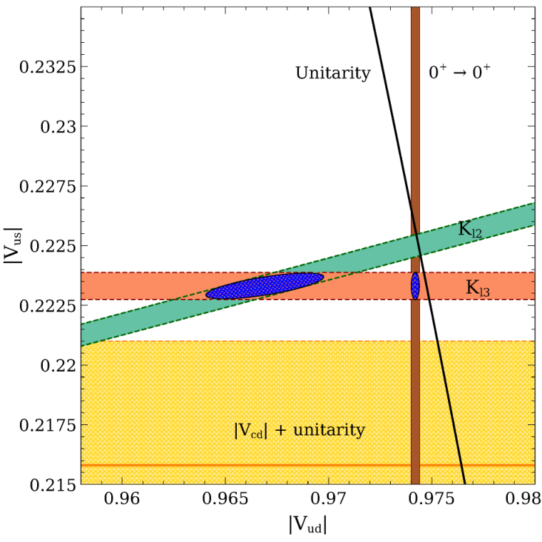
One can perform another test of the unitarity of the CKM matrix by comparing with , which in the SM should be equal up to corrections of , with . Including the corrections, which only affect the last significant digit, the most precise determination of from leptonic decays [49] implies the value . This value of agrees at the level with our result in Eq. (46), although with an uncertainty that is an order of magnitude larger. The uncertainty is dominated by the experimental error on the leptonic decay rate , which is expected to be reduced by BESIII and Belle II. This result is also depicted in Fig. 11. As is the case for our main result, is in tension with first-row CKM unitarity by about when it is used together with from superallowed nuclear decays in Eq. (1).
Note that, in order to perform this test, we change the normalization of the decay constant obtained in Ref. [49] to account for a change in the scale-setting quantity in that work, , from the PDG value [3] to the FLAG average [6]. That gives us .77 7 Although the dependence of on the scale-setting quantity is much more complicated than a simple linear relation, this estimate should capture most of the effect and, thus, be good enough for this comparison, since its uncertainty is dominated by that of the decay rate. The reason for that change is that the PDG value relies on an external input for , which is taken from superallowed nuclear decays, which obscures the comparison. The FLAG number, however, is an average of direct lattice determinations of . With this choice of , the errors are fairly large, and the value of extracted from experimental data on pion leptonic decays [16] agrees within with both from superallowed nuclear decays and the value from kaon decays only that we discuss below.
VII.3 Ratio of leptonic and semileptonic decays
Another way of analyzing the tension between SM kaon leptonic and semileptonic decays is by looking at ratios of decay widths of leptonic and semileptonic decays, where the dependence on cancels. We can construct two ratios
| (50) |
The first ratio does not depend on any CKM matrix elements, while the second one is proportional to . In addition, the short-distance radiative corrections cancel between numerator and denominator in the first ratio, but not in the second.
Taking experimental averages for the kaon decays and assuming the SM, we obtain88 8 We take from Ref. [16], which does not use the same value of the universal short-distance electroweak correction as [7] (from which we take the other experimental averages). The imperfect cancellation is too small to affect the conclusion drawn here. [16, 7]
| (51) |
With our result in Eq. (43) for , the average of lattice calculations for from Ref. [16], from Ref. [49], and from [2], those ratios are.
| (52) |
where we have not taken into account any correlation between the decay constants and the form factor. Comparing Eqs. (51) and (52), we see some tension, and , respectively, between the SM predictions and the experimental measurements. The error from lattice QCD is the main limiting factor in this comparison, but that can be reduced by taking into account the correlation between the numerator and denominator in Eq. (52), which we plan to do in the future.
Alternatively, one can compare the ratio as extracted from experiment and theory to get a value of the CKM matrix element , and compare it with the value from superallowed nuclear decays. The result of such an exercise is , approximately lower than the value from superallowed decays. This result is seen in Fig. 11 at the intersection of the two bands for and . It also deviates from the unitarity condition.
VII.4 Implications of the new extraction of
If the decrease of the central value and uncertainty of the nucleus-independent electroweak radiative corrections involved in the extraction of from superallowed decays in Ref. [19] is confirmed, the new value would exacerbate some of the tensions we have just discussed.
First, as shown above, this value of and our semileptonic result for would imply a greater than violation of first-row CKM unitarity. The tension between our semileptonic value of and the one extracted from kaon leptonic decays and , however, would be slightly reduced to , since a smaller value of would give a smaller value of the leptonic , closer to our semileptonic extraction. For the same reason, the tension between the ratios involving in Eqs. (51) and (52) would be slightly lessened.
In Fig. 12, as an example, we show the comparison of the unitarity prediction for using both and , together with the results in this work. Given the important implications of a value of with a smaller error and a smaller central value, it is very important to confirm the new calculation of radiative corrections in Ref. [19], and to understand the discrepancy with the previous best determination in Ref. [81].

VIII Conclusions and outlook
Using the HISQ MILC ensembles, we have performed the most precise computation to date of the vector form factor at zero momentum transfer, , and the first one to include the dominant FV effects, as calculated in ChPT at NLO. Our result for the form factor enables a direct determination of the CKM matrix element from semileptonic kaon decays with a theory error that is, for the first time, at the same level as the experimental error. Further, the uncertainty in this direct determination is now similar to those from indirect determinations based on leptonic decays with as input.
A key to achieving this level of precision is simulating at near-physical values of the quark masses, which drastically reduces the systematic errors associated with the chiral extrapolation (replacing it with an interpolation), as well as the error coming from the chiral LECs that are inputs to the analysis. The finite-volume effects, one of the main sources of uncertainty in our previous analyses, have also been significantly reduced by explicitly including them at NLO (the leading nontrivial order) in ChPT. The dominant remaining source of error is now statistics, which could be reduced by extending the key ensembles with physical quark masses, and including the existing MILC physical-mass ensemble with a finer lattice spacing of fm.
Another important error arises from the uncertainty in the ChPT LECs of order . That uncertainty could be reduced by performing a combined analysis of form-factor data together with light meson masses and decay constants, which would put more constraints on the ChPT LECs. In particular, the error from is comparable to, but greater than, that from , and the combined analysis could significantly reduce the error. Errors from , , and would also be reduced, but they have a much smaller effect on the total error here.
We find that the extraction of from semileptonic kaon decays is in tension both with the extraction from leptonic kaon decays and with unitarity at the – level. In particular, the unitarity test based only on kaon decay data, without any external input for , and having as nonperturbative inputs from this work and from Ref. [49], shows a tension. While unitarity tests based on are currently limited by the uncertainty in that matrix element, the tension with unitarity would raise to the level if the new calculation of radiative corrections involved in the extraction of from superallowed decays [19] is confirmed.
The test based on kaon-decay data has similarly sized uncertainties arising from both theory and experiment. In order to shed light on these tensions, improvements from both the theoretical and experimental sides are urgently needed, as are improvements in other approaches. A new round of experiments is expected to reduce the experimental error to in the next few years [7]. More importantly, the new high-statistics data will help to check the consistency of current fits, and to perform a more thorough study of systematic errors on the experimental averages.
For the experimental determination of , electromagnetic and isospin effects are currently being estimated using phenomenology and ChPT techniques. Although they are not yet a dominant source of error (EM effects make a 0.11% correction to the individual neutral channels), with the reduction of other sources of error and the forthcoming improvement in the experimentally measured branching ratios and lifetimes, they will eventually need to be included directly in the lattice-QCD simulations. Recent efforts in that direction can be found in Refs. [82, 83, 84, 85].
Isospin corrections are numerically important for the charged kaon channels, where those effects enter already at LO through - mixing. The NNLO ChPT estimate of the corrections for the charged modes has large errors [69] due to the unknown value of the LECs. Fortunately, the experimental average is dominated by the neutral-kaon channels, so the charged-mode uncertainty does not have a large effect on the final experimental average. The strong isospin-breaking correction used in the experimental average is a NLO ChPT estimate that partially includes NNLO effects; it does not include the uncertainty associated with higher-order terms in the chiral expansion. However, the fact that the value used in the average and the one extracted from experiment are so close (2.45(19)% vs. 2.82(38)% [7]), that the result for using only the neutral modes agrees with the one using all decay modes—see Sec. VII.1, and that neutral modes are the dominant ones in the average, indicates that the experimental average using this estimate is robust.
The uncertainties from the phase-space integrals are insignificant at present in the final error for the experimental average. It is therefore not crucial at present to have a better representation of those, i.e., to have the dependence of the form factors. In the future, however, lattice calculations of could provide better determinations of the form factor slope than those relying on experimental data [29, 7].
An important future step in the investigation of the tensions observed in the first-row unitarity relation, and in the value of extracted from different sources, will be to perform a correlated analysis of semileptonic and leptonic kaon decays. That analysis would provide a more precise value of the ratio and potentially give an insight into the tensions. Another key point in the study of those tensions is clarifying the role of the electroweak radiative corrections in the extraction of from superallowed decays, as well as reducing the error of that CKM matrix element as extracted, not only from superallowed decays, but from other sources.
Acknowledgements.
We thank Matthew Moulson for useful discussions and Bipasha Chakraborty for participating in an early stage of this analysis. We thank Johan Bijnens for making his isospin-breaking NLO partially quenched ChPT and isospin-breaking NNLO full QCD codes available to us, and Bijnens and Johan Relefors for making their FV ChPT code available to us. We thank Zechariah Gelzer for discussions on autocorrelations in the MILC ensembles. Computations for this work were carried out with resources provided by the USQCD Collaboration, the National Energy Research Scientific Computing Center, the Argonne Leadership Computing Facility, the Blue Waters sustained-petascale computing project, the National Institute for Computational Science, the National Center for Atmospheric Research, and the Texas Advanced Computing Center. USQCD resources are acquired and operated thanks to funding from the Office of Science of the U.S. Department of Energy. The National Energy Research Scientific Computing Center is a DOE Office of Science User Facility supported by the Office of Science of the U.S. Department of Energy under Contract No. DE-AC02-05CH11231. An award of computer time was provided by the Innovative and Novel Computational Impact on Theory and Experiment (INCITE) program. This research used resources of the Argonne Leadership Computing Facility, which is a DOE Office of Science User Facility supported under Contract DE-AC02-06CH11357. The Blue Waters sustained-petascale computing project is supported by the National Science Foundation (awards OCI-0725070 and ACI-1238993) and the State of Illinois. Blue Waters is a joint effort of the University of Illinois at Urbana-Champaign and its National Center for Supercomputing Applications. This work is also part of the “Lattice QCD on Blue Waters” and “High Energy Physics on Blue Waters” PRAC allocations supported by the National Science Foundation (award numbers 0832315 and 1615006) and used an allocation received under the “Blue Waters for Illinois faculty” program. This work used the Extreme Science and Engineering Discovery Environment (XSEDE), which is supported by National Science Foundation grant number ACI-1548562 [161]. Allocations under the Teragrid and XSEDE programs included resources at the National Institute for Computational Sciences (NICS) at the Oak Ridge National Laboratory Computer Center, The Texas Advanced Computing Center and the National Center for Atmospheric Research, all under NSF teragrid allocation TG-MCA93S002. Computer time at the National Center for Atmospheric Research was provided by NSF MRI Grant CNS-0421498, NSF MRI Grant CNS-0420873, NSF MRI Grant CNS-0420985, NSF sponsorship of the National Center for Atmospheric Research, the University of Colorado, and a grant from the IBM Shared University Research (SUR) program. This work was supported in part by the U.S. Department of Energy under grants No. DE-FG02-91ER40628 (C.B.), No. DE-FC02-12ER41879 (C.D.), No. DE-SC0010120 (S.G.), No. DE-FG02-91ER40661 (S.G.), No. DE-FG02-13ER42001 (A.X.K.), No. DE-SC0015655 (A.X.K.), No. DE-SC0010005 (E.T.N.), No. DE-FG02-13ER41976 (D.T.); by the U.S. National Science Foundation under grants PHY14-14614 and PHY17-19626 (C.D.), PHY14-17805 (J.L.), and PHY13-16748 and PHY16-20625 (R.S.); by the MINECO (Spain) under grants FPA2013-47836-C-1-P and FPA2016-78220-C3-3-P (E.G.); by the Junta de Andalucía (Spain) under grant No. FQM-101 (E.G.); by the European Commission (EC) under Grant No. PCIG10-GA-2011-303781 (E.G.); by the U.K. Science and Technology Facilities Council (J.K.); by the German Excellence Initiative and the European Union Seventh Framework Program under grant agreement No. 291763 as well as the European Union Marie Curie COFUND program (J.K., A.S.K.). Brookhaven National Laboratory is supported by the United States Department of Energy, Office of Science, Office of High Energy Physics, under Contract No. DE-SC0012704. Fermilab is operated by Fermi Research Alliance, LLC, under Contract No. DE-AC02-07CH11359 with the United States Department of Energy, Office of Science, Office of High Energy Physics.References
- [1] M. González-Alonso and J. Martin Camalich, JHEP 1612, 052 (2016) [arXiv:1605.07114 [hep-ph]].
- [2] J. C. Hardy and I. S. Towner, arXiv:1807.01146 [nucl-ex].
- [3] C. Patrignani et al. [Particle Data Group], Chin. Phys. C 40 (2016), 100001.
- [4] D. Počanić et al., Phys. Rev. Lett. 93, 181803 (2004) [hep-ex/0312030].
- [5] D. Počanić, talk at the Ninth International Workshop on the CKM Unitarity Triangle (May 2016, Mumbai), https://indico.tifr.res.in/indico/contributionDisplay.py?contribId=46&confId=5095
- [6] S. Aoki et al. [Flavour Lattice Averaging Group], Eur. Phys. J. C 77 (2017), 112 [arXiv:1607.00299 [hep-lat]], and updates at http://flag.unibe.ch/.
- [7] M. Moulson, PoS CKM 2016, 033 (2017) [arXiv:1704.04104 [hep-ex]].
- [8] S. Dürr et al., Phys. Rev. D 95 (2017), 054513 [arXiv:1601.05998 [hep-lat]].
- [9] N. Carrasco et al. [ETM Collaboration], Phys. Rev. D 91 (2015), 054507 [arXiv:1411.7908 [hep-lat]].
- [10] T. Blum et al. [RBC and UKQCD Collaborations], Phys. Rev. D 93 (2016), 074505 [arXiv:1411.7017 [hep-lat]].
- [11] A. Bazavov et al. [Fermilab Lattice and MILC Collaborations], Phys. Rev. D 90 (2014), 074509 [arXiv:1407.3772 [hep-lat]].
- [12] R. J. Dowdall, C. T. H. Davies, G. P. Lepage, and C. McNeile [HPQCD Collaboration], Phys. Rev. D 88 (2013) 074504 [arXiv:1303.1670 [hep-lat]].
- [13] A. Bazavov et al. [MILC Collaboration], PoS LATTICE 2010 (2010) 074 [arXiv:1012.0868 [hep-lat]].
- [14] S. Dürr et al. [Budapest-Marseille-Wuppertal Collaboration], Phys. Rev. D 81 (2010) 054507 [arXiv:1001.4692 [hep-lat]].
- [15] E. Follana et al. [HPQCD Collaboration], Phys. Rev. Lett. 100 (2008) 062002 [arXiv:0706.1726 [hep-lat]].
- [16] J. L. Rosner, S. Stone, and R. S. Van de Water, in Review of Particle Physics [3] arXiv:1509.02220 [hep-ph].
- [17] V. Cirigliano, H. Neufeld and H. Pichl, Eur. Phys. J. C 35, 53 (2004) [hep-ph/0401173].
- [18] V. Cirigliano, M. Knecht, H. Neufeld, H. Rupertsberger and P. Talavera, Eur. Phys. J. C 23, 121 (2002) [hep-ph/0110153].
- [19] C. Y. Seng, M. Gorchtein, H. H. Patel, and M. J. Ramsey-Musolf, Phys. Rev. Lett. 121 (2018) no.24, 241804 [arXiv:1807.10197 [hep-ph]].
- [20] N. Cabibbo, E. C. Swallow, and R. Winston, Phys. Rev. Lett. 92 (2004) 251803 [hep-ph/0307214].
- [21] V. Cirigliano, G. Ecker, H. Neufeld, A. Pich, and J. Portolés, Rev. Mod. Phys. 84, 399 (2012) [arXiv:1107.6001 [hep-ph]].
- [22] A. Sirlin, Rev. Mod. Phys. 50, 573 (1978); (E) 50, 905 (1978).
- [23] A. Sirlin, Nucl. Phys. B 196, 83 (1982).
- [24] W. J. Marciano and A. Sirlin, Phys. Rev. Lett. 71, 3629 (1993).
- [25] V. Cirigliano, M. Giannotti, and H. Neufeld, JHEP 0811 (2008) 006 [arXiv:0807.4507 [hep-ph]].
- [26] A. Bazavov et al. [Fermilab Lattice and MILC Collaborations], Phys. Rev. Lett. 112 (2014), 112001 [arXiv:1312.1228 [hep-ph]].
- [27] E. Gámiz et al. [Fermilab Lattice and MILC Collaborations], PoS LATTICE 2013 (2014) 395 [arXiv:1311.7264 [hep-lat]].
- [28] P. A. Boyle et al. [RBC and UKQCD Collaborations], JHEP 1506 (2015) 164 [arXiv:1504.01692 [hep-lat]].
- [29] N. Carrasco, P. Lami, V. Lubicz, L. Riggio, S. Simula, and C. Tarantino [ETM Collaboration], Phys. Rev. D 93 (2016), 114512 [arXiv:1602.04113 [hep-lat]].
- [30] A. Bazavov et al. [Fermilab Lattice and MILC Collaborations], Phys. Rev. D 87, 073012 (2013) [arXiv:1212.4993 [hep-lat]].
- [31] P. A. Boyle, J. M. Flynn, N. Garron, A. Jüttner, C. T. Sachrajda, K. Sivalingam, and J. M. Zanotti [RBC and UKQCD Collaborations], JHEP 1308, 132 (2013) [arXiv:1305.7217 [hep-lat]].
- [32] P. A. Boyle et al. [RBC and UKQCD Collaborations], Eur. Phys. J. C 69, 159 (2010) [arXiv:1004.0886 [hep-lat]].
- [33] S. Aoki et al. [JLQCD Collaboration], Phys. Rev. D 96, no. 3, 034501 (2017) [arXiv:1705.00884 [hep-lat]].
- [34] T. Primer et al. [Fermilab Lattice and MILC Collaborations], PoS LATTICE 2014, 374 (2014) [arXiv:1411.1651 [hep-lat]].
- [35] E. Gámiz et al. [Fermilab Lattice and MILC Collaborations], PoS LATTICE 2016 (2016) 286 [arXiv:1611.04118 [hep-lat]].
- [36] V. Mateu and A. Pich, JHEP 0510 (2005) 041 [hep-ph/0509045].
- [37] E. Gámiz, M. Jamin, A. Pich, J. Prades, and F. Schwab, Phys. Rev. Lett. 94 (2005) 011803 [hep-ph/0408044].
- [38] M. Antonelli, V. Cirigliano, A. Lusiani and E. Passemar, JHEP 1310 (2013) 070 [arXiv:1304.8134 [hep-ph]].
- [39] R. J. Hudspith, R. Lewis, K. Maltman and J. Zanotti, Phys. Lett. B 781, 206 (2018) [arXiv:1702.01767 [hep-ph]].
- [40] P. Boyle et al. [RBC and UKQCD Collaborations], arXiv:1803.07228 [hep-lat].
- [41] E. Kou et al., arXiv:1808.10567 [hep-ex].
- [42] Y. Amhis et al. [HFLAV Collaboration], Eur. Phys. J. C 77 (2017), 895 [arXiv:1612.07233 [hep-ex]], and updates at https://hflav.web.cern.ch/.
- [43] C. Bernard, J. Bijnens, E. Gámiz, and J. Relefors, JHEP 1703, 120 (2017) [arXiv:1702.03416 [hep-lat]].
- [44] C. Bernard and D. Toussaint [MILC Collaboration], Phys. Rev. D 97, 074502 (2018), [arXiv:1707.05430 [hep-lat]].
- [45] H. Na, C. T. H. Davies, E. Follana, P. Lepage, and J. Shigemitsu, PoS LAT 2009 (2009) 247 [arXiv:0910.3919 [hep-lat]].
- [46] J. Koponen et al. [HPQCD Collaboration], arXiv:1208.6242 [hep-lat].
- [47] A. Bazavov et al. [MILC Collaboration], Phys. Rev. D 82, 074501 (2010) [arXiv:1004.0342 [hep-lat]].
- [48] A. Bazavov et al. [MILC Collaboration], Phys. Rev. D 87, 054505 (2013) [arXiv:1212.4768 [hep-lat]].
- [49] A. Bazavov et al., Phys. Rev. D 98 (2018) no.7, 074512 [arXiv:1712.09262 [hep-lat]].
- [50] E. Follana et al. [HPQCD and UKQCD Collaborations], Phys. Rev. D 75 (2007) 054502 [hep-lat/0610092].
- [51] C. McNeile et al. [UKQCD Collaboration], Phys. Rev. D 73, 074506 (2006) [hep-lat/0603007].
- [52] H. Na, C. T. H. Davies, E. Follana, G. P. Lepage, and J. Shigemitsu [HPQCD Collaboration], Phys. Rev. D82 (2010) 114506. [arXiv:1008.4562 [hep-lat]].
- [53] A. Bazavov et al. [Fermilab Lattice and MILC Collaborations], Phys. Rev. D 93, no. 11, 113016 (2016) [arXiv:1602.03560 [hep-lat]].
- [54] E. Gámiz et al. [Fermilab Lattice and MILC Collaborations], PoS LATTICE 2012, 113 (2012) [arXiv:1211.0751 [hep-lat]].
- [55] A. Bazavov et al. [MILC Collaboration], Phys. Rev. D 81, 114501 (2010), [arXiv:1003.5695].
- [56] R. Brower, S. Chandrasekharan, J. W. Negele, and U. J. Wiese, Phys. Lett. B 560, 64 (2003) [hep-lat/0302005].
- [57] S. Aoki, H. Fukaya, S. Hashimoto, and T. Onogi, Phys. Rev. D 76, 054508 (2007) [arXiv:0707.0396 [hep-lat]].
- [58] A. Bazavov et al. [Fermilab Lattice and MILC and TUMQCD Collaborations], Phys. Rev. D 98 (2018) no.5, 054517 [arXiv:1802.04248 [hep-lat]].
- [59] M. Ademollo and R. Gatto, Phys. Rev. Lett. 13, 264 (1964).
- [60] C. Bernard, J. Bijnens, and E. Gámiz, Phys. Rev. D 89 (2014), 054510 [arXiv:1311.7511 [hep-lat]].
- [61] J. Bijnens and P. Talavera, Nucl. Phys. B669 (2003) 341-362. [hep-ph/0303103].
- [62] H. W. Fearing and S. Scherer, Phys. Rev. D 53, 315 (1996) [hep-ph/9408346].
- [63] J. Bijnens, G. Colangelo, and G. Ecker, JHEP 9902 (1999) 020 [hep-ph/9902437].
- [64] A. Bazavov et al., Rev. Mod. Phys. 82 (2010) 1349-1417.
- [65] A. Bazavov et al. [Fermilab Lattice and MILC Collaborations], Phys. Rev. D 85, 114506 (2012) [arXiv:1112.3051 [hep-lat]].
- [66] A. Bazavov et al. [Fermilab Lattice and MILC Collaborations], Phys. Rev. D 90 (2014), 074509 [arXiv:1407.3772 [hep-lat]].
- [67] J. Bijnens and G. Ecker, Ann. Rev. Nucl. Part. Sci. 64 (2014) 149 [arXiv:1405.6488 [hep-ph]].
- [68] A. Bazavov et al. [MILC Collaboration], PoS LATTICE 2011 (2011) 107 [arXiv:1111.4314 [hep-lat]], and updates by N. Brown (private communication).
- [69] J. Bijnens and K. Ghorbani, arXiv:0711.0148 [hep-ph].
- [70] C. Bernard et al., Phys. Rev. D 62, 034503 (2000) [hep-lat/0002028].
- [71] R. Sommer, Nucl. Phys. B 411, 839 (1994) [hep-lat/9310022].
- [72] J. Gasser and H. Leutwyler, Nucl. Phys. B 250, 517 (1985).
- [73] H. Leutwyler and A. V. Smilga, Phys. Rev. D 46 (1992) 5607.
- [74] B. Billeter, C. E. Detar, and J. Osborn, Phys. Rev. D 70, 077502 (2004) [hep-lat/0406032].
- [75] S. Basak et al. [MILC Collaboration], Phys. Rev. D 99 (2019) no.3, 034503 [arXiv:1807.05556 [hep-lat]].
- [76] G. Ecker, PoS CD 15, 011 (2015) [arXiv:1510.01634 [hep-ph]].
- [77] A. Kastner and H. Neufeld, Eur. Phys. J. C 57, 541 (2008) [arXiv:0805.2222 [hep-ph]].
- [78] V. Cirigliano, G. Ecker, M. Eidemüller, R. Kaiser, A. Pich, and J. Portolés, JHEP 0504, 006 (2005) [hep-ph/0503108].
- [79] M. Jamin, J. A. Oller, and A. Pich, JHEP 0402, 047 (2004) [hep-ph/0401080].
- [80] H. Leutwyler and M. Roos, Z. Phys. C 25, 91 (1984).
- [81] W. J. Marciano and A. Sirlin, Phys. Rev. Lett. 96 (2006) 032002 [hep-ph/0510099].
- [82] N. Carrasco, V. Lubicz, G. Martinelli, C. T. Sachrajda, N. Tantalo, C. Tarantino, and M. Testa, Phys. Rev. D 91 (2015), 074506 [arXiv:1502.00257 [hep-lat]].
- [83] D. Giusti, V. Lubicz, G. Martinelli, C. T. Sachrajda, F. Sanfilippo, S. Simula, N. Tantalo and C. Tarantino, Phys. Rev. Lett. 120 (2018) no.7, 072001 [arXiv:1711.06537 [hep-lat]].
- [84] A. Patella, PoS LATTICE 2016 (2017) 020 [arXiv:1702.03857 [hep-lat]].
- [85] D. Giusti, V. Lubicz, G. Martinelli, C. Sachrajda, F. Sanfilippo, S. Simula and N. Tantalo, PoS LATTICE 2018, 266 (2019) [arXiv:1811.06364 [hep-lat]].