่ทณๅˆฐ่ฎบๆ–‡ๆญฃๆ–‡
W Papers็‹ฌ็ซ‹่ฎบๆ–‡้˜…่ฏปๅ™จ arXiv:1809.02443 ่ฎบๆ–‡ๆญฃๆ–‡ ่ฎก็ฎ—้˜…่ฏปๆ—ถ้—ด ยท 0%
ๅผ•็”จ่ฟ™็ฏ‡่ฎบๆ–‡ๆ นๆฎๅฝ“ๅ‰่ฎบๆ–‡ๅ…ƒๆ•ฐๆฎ็”Ÿๆˆ๏ผŒๆญฃๅผๆŠ•็จฟๅ‰ๅปบ่ฎฎๆ ธๅฏนใ€‚


License: arXiv.org perpetual non-exclusive license
arXiv:1809.02443v3 [math.ST] 16 Nov 2020

Posterior analysis of nn in the binomial (n,p)(n,p) problem with both parameters unknown - with applications to quantitative nanoscopy

Johannes Schmidt-Hieber??,?? โ€ƒโ€ƒ Laura Fee Schneider??,?? โ€ƒโ€ƒ Thomas Staudt??,?? โ€ƒโ€ƒ Andrea Krajina?? โ€ƒโ€ƒ Timo Aspelmeier?? โ€ƒโ€ƒ Axel Munk??

University of Gรถttingen?? and University of Twente??

Estimation of the population size nn from kk i.i.d. binomial observations with unknown success probability pp is relevant to a multitude of applications and has a long history. Without additional prior information this is a notoriously difficult task when pp becomes small, and the Bayesian approach becomes particularly useful. For a large class of priors, we establish posterior contraction and a Bernstein-von Mises type theorem in a setting where pโ†’0p\rightarrow 0 and nโ†’โˆžn\rightarrow\infty as kโ†’โˆžk\to\infty. Furthermore, we suggest a new class of Bayesian estimators for nn and provide a comprehensive simulation study in which we investigate their performance. To showcase the advantages of a Bayesian approach on real data, we also benchmark our estimators in a novel application from super-resolution microscopy.

MSC 2010 subject classifications: primary 62G05; secondary 62F15,62F12, 62P10, 62P35
Keywords: Bayesian estimation, posterior contraction, Bernstein-von Mises theorem, binomial distribution, beta-binomial likelihood, quantitative cell imaging

1 Introduction

The binomial distribution with parameters nn and pp is the most fundamental model for the repetition of independent success/failure events. Motivated by several important applications, we focus on the situation where both pp and nn are unknown. For example, nn might corresponds to the population size of a certain species (Otis et al., 1978; Royle, 2004; Raftery, 1988), the number of defective appliances (Draper and Guttman, 1971), or the number of faults in software reliability (Basu and Ebrahimi, 2001). In Section 4 we elaborate on a novel application where nn is the number of unknown fluorescent markers in quantitative super-resolution microscopy (Betzig et al., 2006; Hell, 2009; Aspelmeier et al., 2015).

The joint estimation of the population size nn and the success probability pp of a binomial distribution from kk independent observations has a long history dating back at least to Fisher (1941). In comparison to the estimation of one of the parameters when the other is known (Lehmann and Casella, 1996), this problem turns out to be much harder. Fisher, who regarded the assumption of an unknown integer nn as โ€œentirely academicโ€, suggested the use of the sample maximum, arguing that this estimator is necessarily good if the sample size is sufficiently large. Indeed, if X1,โ€ฆ,XkX_{1},\dots,X_{k} are i.i.d. Binโก(n,p)\operatorname{Bin}(n,p) distributed random variables for fixed nโˆˆโ„•n\in\mathbb{N} and pโˆˆ(0,1)p\in(0,1), the sample maximum Mk:=maxi=1,โ€ฆ,kโกXiM_{k}:=\max_{i=1,\ldots,k}X_{i} converges exponentially fast to nn as kโ†’โˆž,k\rightarrow\infty, since

โ„™โก(Mk=n)=1โˆ’โ„™โก(maxi=1,โ€ฆ,kโกXi<n)=1โˆ’(1โˆ’pn)k.\mathbb{P}\big(M_{k}=n\big)=1-\mathbb{P}\big(\max_{i=1,\ldots,k}X_{i}<n\big)=1-(1-p^{n})^{k}. (1.1)

In practice, however, the regime with small pp (โ€œrare eventsโ€) is often the relevant one (see the references below and Section 4). In this setting, the sample maximum strongly underestimates the true nn even for large sample sizes k.k. This is explicitly quantified in DasGupta and Rubin (2005): if p=0.1p=0.1 and n=10n=10, then the sample size kk needs to be larger than 36353635 to ensure โ„™โก(Mkโ‰ฅn/2)โ‰ฅ1/2\mathbb{P}(M_{k}\geq n/2)\geq 1/2. If p=0.1p=0.1 and n=20n=20, one would even need a sample size of more than k=900โ€‰000k=900\,000 for the same probability.

The erratic behavior of the sample maximum can be explored by allowing the parameters nn and pp to depend on kk. Applying Bernoulliโ€™s inequality and the bound 1โˆ’xโ‰คeโˆ’x1-x\leq e^{-x}, it follows from (1.1) that 1โˆ’eโˆ’kโ€‹pnโ‰คโ„™โก(Mk=n)โ‰คkโ€‹pn1-e^{-kp^{n}}\leq\mathbb{P}(M_{k}=n)\leq kp^{n}. Therefore, the sample maximum MkM_{k} becomes an inconsistent estimator of nn if kโ€‹pnโ†’0kp^{n}\rightarrow 0 as kโ†’โˆžk\to\infty (see Lemma 3 for a characterization of domains of consistency and inconsistency of MkM_{k}). One particular example where consistency breaks down is the domain of attraction of the Poisson distribution: when nโ‰ฅlogโก(k)โ†’โˆžn\geq\log(k)\rightarrow\infty and pโ†’0p\rightarrow 0 such that nโ€‹pโ†’ฮผโˆˆ(0,โˆž)np\rightarrow\mu\in(0,\infty), then kโ€‹pnโ‰คk1+logโกpโ†’0kp^{n}\leq k^{1+\log p}\to 0. In this case, Binโก(n,p)\operatorname{Bin}(n,p) approaches the Poisson distribution with intensity parameter ฮผ\mu, leading to non-identifiability of the parameters (n,p)(n,p) in the limit. Consequently, more refined estimation techniques become necessary.

Since Fisher (1941), a variety of methods have been proposed to improve upon the sample maximum. A definite answer, however, remains elusive until today. The general lesson from the attempts to obtain better estimators in the small pp regime is that further information on nn and pp is required, which calls for a Bayesian approach. An early Bayesian estimator of the binomial parameters dates back to Draper and Guttman (1971), who suggested to use the posterior mode under a uniform prior for nn (upper bounded by some maximal value), and a Betaโก(a,b)\operatorname{Beta}(a,b) prior for pp with a,b>0a,b>0. Later, Raftery (1988), Gรผnel and Chilko (1989), Hamedani and Walter (1988), and Berger et al. (2012), besides others, considered different Bayesian estimators. Raftery (1988), for example, introduced a hierarchical Bayes approach that utilizes a Poisson prior on nn with intensity parameter ฮป>0\lambda>0 and a uniform prior distribution on [0,1][0,1] for pp. Under the choice ฯ€โก(ฮป)โˆผ1/ฮป\pi(\lambda)\sim 1/\lambda as hyperprior, this hierarchical approach is equivalent to choosing the (improper) scale prior 1/n1/n for nn. This prior is also recommended as an objective prior for nn in Berger et al. (2012). A broader perspective on objective priors for discrete parameter spaces is offered in Villa and Walker (2014); Villa and Walker (2015), who propose a prior on n|pn\,|\,p that depends on the Kullback-Leibler divergence between two successive values of nn. The Villa-Walker construction therefore also models the dependency between nn and p.p.

Besides considering the posterior mode and posterior median as estimators, Raftery (1988) suggested to minimize the Bayes risk with respect to the relative quadratic loss. From extensive simulation studies (see the aforementioned references and Section 3 of this article), it is understood that these Bayesian estimators generally deliver good results, especially when compared to frequentist approaches. To the best of our knowledge, however, there is no rigorous theoretical underpinning of these findings. In particular, little is known about the posterior concentration of such estimators, and no systematic understanding of the role of the prior has been established.

Our contribution to this topic is threefold. First (i), we propose a new class of Bayesian estimators for nn, generalizing the approach in Raftery (1988). Secondly (ii), we analyze the asymptotic behavior of the posterior distribution of nn for a large class of priors and asymptotic regimes. This includes statements of posterior consistency as well as a novel Bernstein-von Mises type theorem. Finally (iii), we extend the i.i.d. Binโก(n,p)\operatorname{Bin}(n,p) model to a regression setting and apply the suggested estimators to count the number of fluorophores from super-resolution images. This is a difficult issues of quantitative biology and a target of ongoing research.

Ad (i)

We consider product priors of the form ฮ nโŠ—ฮ p\Pi_{n}\otimes\Pi_{p} on (n,p)(n,p) with ฮ pโˆผBetaโก(a,b)\Pi_{p}\sim\operatorname{Beta}(a,b) for some a,b>0a,b>0 and ฮ nโ€‹(n)โˆnโˆ’ฮณ\Pi_{n}(n)\propto n^{-\gamma} for all nโˆˆโ„•n\in\mathbb{N} and some ฮณ>1\gamma>1. Independence of nn and pp in the prior is a natural assumption and can be justified in our application based on physical considerations (Section 4). The beta prior for pp is the standard choice and makes the problem analytically tractable due to its conjugacy property (Draper and Guttman, 1971). The priors nโˆ’ฮณn^{-\gamma} for nn, which we call scale priors with scaling parameter ฮณ\gamma, are widely studied in the literature on the binomial (n,p)(n,p) problem and its variations, see (Raftery, 1988; Berger et al., 2012; Link, 2013; Wang et al., 2007; Tancredi et al., 2020).

Based on these prior choices, we focus on two Bayesian scale estimators for nn. The first is the posterior mode estimator n^pm\hat{n}_{\mathrm{pm}} and the second is the Bayes estimator n^rql\hat{n}_{\mathrm{rql}} with respect to the relative quadratic loss, โ„“โก(x,y)=(x/yโˆ’1)2\ell(x,y)=(x/y-1)^{2}. Following Raftery (1988), the respective estimators are given by

n^pm\displaystyle\hat{n}_{\mathrm{pm}} =argโ€‹maxnโ‰ฅMkโกLa,bโ€‹(n)nฮณ,\displaystyle=\mathop{\rm arg\max}_{n\geq M_{k}}\frac{L_{a,b}(n)}{n^{\gamma}}, (1.2a)
n^rql\displaystyle\hat{n}_{\mathrm{rql}} =๐”ผโก[1n|๐—k]๐”ผโก[1n2|๐—k]=โˆ‘n=Mkโˆž1n1+ฮณโ€‹La,bโ€‹(n)โˆ‘n=Mkโˆž1n2+ฮณโ€‹La,bโ€‹(n),\displaystyle=\frac{\mathbb{E}\left[\frac{1}{n}|\mathbf{X}^{k}\right]}{\mathbb{E}\left[\frac{1}{n^{2}}|\mathbf{X}^{k}\right]}=\frac{\sum_{n=M_{k}}^{\infty}\frac{1}{n^{1+\gamma}}L_{a,b}(n)}{\sum_{n=M_{k}}^{\infty}\frac{1}{n^{2+\gamma}}L_{a,b}(n)}, (1.2b)

where ๐—k=(X1,โ€ฆ,Xk)\mathbf{X}^{k}=(X_{1},\ldots,X_{k}) denotes the data vector and La,bโ€‹(n)L_{a,b}(n) is the (data dependent) beta-binomial likelihood defined in equation (2.1) below (see also Carroll and Lombard (1985)). In our applications (Section 3 and 4), we assume n^pm\hat{n}_{\mathrm{pm}} and n^rql\hat{n}_{\mathrm{rql}} to be integer valued by taking the argโ€‹max\mathop{\rm arg\max} over โ„•\mathbb{N} and by rounding n^rql\hat{n}_{\mathrm{rql}} to the nearest integer.

Ad (ii)

We provide asymptotic conditions under which the marginal posterior for nn concentrates all mass around the true population size. As before, we assume product priors on (n,p)(n,p) with a beta prior on pp. For nn, we allow general proper priors that decay at most polynomially,

ฮ nโ€‹(n)โ‰ฅฮฒโ€‹nโˆ’ฮฑ,\Pi_{n}(n)\geq\beta n^{-\alpha}, (1.3)

for all nโˆˆโ„•n\in\mathbb{N} and some ฮฑ>1\alpha>1 and ฮฒ>0\beta>0. To investigate the asymptotic behavior of the posterior distribution, we let nn and pp depend on the sample size kk. We formalize this by considering parameter domains of the form

โ„ณk(ฮป):={(n,p):1ฮปโ‰คnpโ‰คฮป,nโ‰คฮปklog6โก(k)},\displaystyle\mathcal{M}_{k}(\lambda):=\left\{(n,p)\,\colon\,\frac{1}{\lambda}\leq np\leq\lambda,\ n\leq\lambda\,\frac{\sqrt{k}}{\log^{6}(k)}\right\}, (1.4)

where ฮป>1\lambda>1 can be chosen arbitrarily. This class describes binomial variables Binโก(n,p)\mathrm{Bin}(n,p) with expectation values nโ€‹pnp bounded away from 00 and infinity, such that nn grows (at most) slightly slower than k\sqrt{k}. Under the condition that ฮ n\Pi_{n} satisfies (1.3), posterior contraction around the true population size n0n_{0} is studied in Theorem 1. If n0n_{0} does not grow faster than k1/4/logโก(k)k^{1/4}/\log(k), we will see that the posterior mass eventually concentrates on the true n0n_{0}. In Theorem 2, we then extend our analysis to a different asymptotic domain in which the true population size n0n_{0} stays bounded but p0p_{0} is allowed to decay. Lower bounds that we establish in Theorem 3 guarantee that the rates for consistency in Theorem 1 and 2 are indeed sharp up to logarithmic factors. We also derive a Bernstein-von Mises type result for the posterior on nn in Theorem 4, which shows that the limit distribution can be viewed as a discretized version of a normal distribution.

The main building block underlying the recent advances in the frequentist analysis of posterior concentration are the connection to posterior mass conditions and the existence of separating statistical test, see Schwartz (1965); Ghosal et al. (2000); Ghosal and van der Vaart (2017). To establish model selection properties of the posterior requires typically different tools (Castillo and van der Vaart, 2012; Castillo et al., 2015; Gao et al., 2020). Since proving that the posterior concentrates on the true population size can be viewed as posterior model selection, it is not surprising that we do not follow the standard posterior contraction proof technique. In fact, a much more refined analysis of the likelihood is necessary and we crucially rely on a decomposition of the log-likelihood via a telescoping sum that is due to Hall (1994). The main challenge in our approach consists of obtaining uniform results over parameter classes where nโ†’โˆžn\to\infty and pโ†’0p\to 0 is allowed (in order to capture the small pp regime). For fixed nn and pp as kโ†’โˆžk\to\infty, in contrast, posterior consistency already follows from Doobโ€™s consistency theorem, see van der Vaart (1998).

Ad (iii)

Modern cell microscopy allows researchers to observe the activity and interactions of biomolecules in unprecedented detail. Especially since the development of super-resolution nanoscopy, for which the 2014 Nobel Prize in Chemistry was awarded, it has become an indispensable tool for understanding the biochemical function of proteins (see Hell (2015) for a survey). Super-resolution techniques rely on photon counts obtained from fluorescent markers (or fluorophores), which are tagged to the specific protein of interest and excited by a laser beam. In this article, we are concerned with single marker switching (SMS) microscopy (Betzig et al., 2006; Rust et al., 2006; Hess et al., 2006; Fรถlling et al., 2008) where the activation of fluorophores and the emission of photons is inherently random: after excitation by a laser, a fluorophore undergoes a complicated cycling through (typically unknown) quantum mechanical states on different time scales. This severely hinders a precise determination of the number of molecules at a certain spot in the specimen, see, e.g., Lee et al. (2012), Rollins et al. (2015), Aspelmeier et al. (2015), Staudt et al. (2020). In Section 4 we show how the number of fluorophores can be obtained from a modified binomial (n,p)(n,p) model. A common difficulty in such experiments is that the number of active markers decreases over the measurement process due to bleaching effects. We show that the initial number n0n_{0} can still be inferred from observations at later time points by linking them through an exponential decay. This leads to a variant of the binomial (n,p)(n,p) model where the bleaching probability of a fluorophore can be estimated jointly with n0n_{0}. We apply this model to experimental data and determine the number of fluorophores on DNA origami test beds.

Outline

This paper is organized as follows. Our results on posterior contraction and the Bernstein-von Mises type theorem can be found in Section 2. For a broader perspective, we also discuss previous results on the asymptotics of several frequentist estimators for nn. Section 3 contains an extensive simulation study in which we examine the posterior of nn for moderate to large kk and compare the finite sample properties of several Bayesian and frequentist estimators. Furthermore, we study the choice of suitable scale priors in different settings and investigate robustness against model deviations from the Bin(n,p)(n,p) model. In Section 4, we apply our estimators to data from super-resolution microscopy. The proof of our main posterior contraction result (Theorem 1) and some auxiliary results about binomial random variables are collected in Section 5. Further proofs as well as additional figures are deferred to the supplementary material.

2 Asymptotic results

Recall that we observe kk independent random variables X1,โ€ฆ,XkX_{1},\dots,X_{k} with Binโก(n,p)\operatorname{Bin}(n,p) distribution. We refer to this setting as the binomial (n,p)(n,p) model. The joint distribution of the data ๐—k=(X1,โ€ฆ,Xk)\mathbf{X}^{k}=(X_{1},\ldots,X_{k}) is denoted by โ„™n,p\mathbb{P}_{n,p} and the expectation with respect to this distribution is ๐”ผn,p\mathbb{E}_{n,p}. We study product priors ฮ nโŠ—ฮ p\Pi_{n}\otimes\Pi_{p} on (nn,pp) and set ฮ p=Betaโก(a,b)\Pi_{p}=\operatorname{Beta}(a,b) with parameters a,b>0a,b>0. The prior ฮ n\Pi_{n} for nn can be chosen as any proper probability distribution on the positive integers such that condition (1.3) holds for some ฮฑ>1\alpha>1 and ฮฒ>0\beta>0. We write Mk=maxi=1,โ€ฆ,kโกXiM_{k}=\max_{i=1,\ldots,k}X_{i} for the sample maximum and Sk=โˆ‘i=1kXi\smash{S_{k}=\sum_{i=1}^{k}X_{i}} for the sample sum. The true parameter values are denoted by n0n_{0} and p0p_{0}.

For a measurable set AโІ[0,1]A\subseteq[0,1] and nโˆˆโ„•n\in\mathbb{N}, the joint posterior distribution for (p,n)(p,n) is given by

ฮ โก(pโˆˆA,n|๐—k)=\displaystyle\Pi\big(p\in A,n\,|\,\mathbf{X}^{k}\big)=
โˆซAtSk+aโˆ’1โ€‹(1โˆ’t)kโ€‹nโˆ’Sk+bโˆ’1โ€‹๐‘‘tโ‹…โˆi=1k(nXi)โ‹…ฮ nโ€‹(n)โˆ‘m=1โˆžโˆซ01tSk+aโˆ’1โ€‹(1โˆ’t)kโ€‹mโˆ’Sk+bโˆ’1โ€‹๐‘‘tโ‹…โˆi=1k(mXi)โ‹…ฮ nโ€‹(m)\displaystyle\quad\qquad\qquad\qquad\frac{\int_{A}t^{S_{k}+a-1}(1-t)^{kn-S_{k}+b-1}\mathrm{d}t\cdot\prod_{i=1}^{k}\binom{n}{X_{i}}\cdot\Pi_{n}(n)}{\sum_{m=1}^{\infty}\int_{0}^{1}t^{S_{k}+a-1}(1-t)^{km-S_{k}+b-1}\mathrm{d}t\cdot\prod_{i=1}^{k}\binom{m}{X_{i}}\cdot\Pi_{n}(m)}

if nโ‰ฅMkn\geq M_{k} and ฮ โก(pโˆˆA,n|๐—k)=0\Pi(p\in A,n\,|\,\mathbf{X}^{k})=0 otherwise. The marginal posterior distribution of nn is thus

ฮ (n|๐—k)โˆโˆi=1k(nXi)โ€‹ฮ“โก(kโ€‹nโˆ’Sk+b)โ€‹ฮ“โ€‹(Sk+a)ฮ“โก(kโ€‹n+a+b)โ€‹โ€‰1โ€‹(nโ‰ฅMk)โŸ=:La,bโ€‹(n)ฮ n(n),\Pi\big(n\,|\,\mathbf{X}^{k}\big)\propto\underbrace{\prod_{i=1}^{k}\binom{n}{X_{i}}\frac{\Gamma(kn-S_{k}+b)\,\Gamma(S_{k}+a)}{\Gamma(kn+a+b)}\,\mathbf{1}(n\geq M_{k})}_{=:\,L_{a,b}(n)}\Pi_{n}(n), (2.1)

where ฮ“\Gamma is the Gamma function, ๐Ÿ\mathbf{1} the indicator function, and La,bL_{a,b} the beta-binomial likelihood.

Posterior contraction

Our first result establishes uniform posterior concentration around the true value n0n_{0} over parameters in the set โ„ณkโ€‹(ฮป)\mathcal{M}_{k}(\lambda) defined in equation (1.4).

Theorem 1.

Consider the binomial (n,p)(n,p) model under the prior mass condition (1.3). For fixed ฮป>1\lambda>1 and kโ†’โˆžk\to\infty,

sup(n0,p0)โˆˆโ„ณkโ€‹(ฮป)๐”ผn0,p0[ฮ (n:|nโˆ’n0|โ‰ฅn02โ€‹log7/4โก(k)k|๐—k)]โ†’0.\sup_{(n_{0},p_{0})\in\mathcal{M}_{k}(\lambda)}\mathbb{E}_{n_{0},p_{0}}\!\left[\Pi\left(n:\left|n-n_{0}\right|\geq\frac{n_{0}^{2}\,\log^{7/4}(k)}{\sqrt{k}}\ \bigg|\,\mathbf{X}^{k}\right)\right]\rightarrow 0. (2.2)

Equivalently, this result could also be stated in terms of the relative loss โ„“โก(n,n0)=|n/n0โˆ’1|2\ell(n,n_{0})=|n/n_{0}-1|^{2}, which is widely studied in the Bayesian literature for this and related problems, see Smith (1988). A noteworthy consequence of Theorem 1 is that the posterior of nn eventually places all mass on the true population size n0n_{0} if the parameters (n0,p0)โˆˆโ„ณkโ€‹(ฮป)(n_{0},p_{0})\in\mathcal{M}_{k}(\lambda) additionally satisfy

n02<klog7/4โก(k).n_{0}^{2}<\frac{\sqrt{k}}{\log^{7/4}(k)}. (2.3)

An inspection of the proof of Theorem 1 reveals that the lower bound on the prior mass condition (1.3) only has to hold for the true value n0n_{0}. If we consider sequences of (proper) priors ฮ n,k\Pi_{n,k} for nn that can change with the sample size kk, it can readily be seen from bound (5.14) in the proof that the assertion of the theorem also holds if ฮ n,kโ€‹(n)โ‰ฅฮฒ/(nโ€‹k)ฮฑ\Pi_{n,k}(n)\geq\beta/(nk)^{\alpha} for all positive integers nโ‰คฮปโ€‹k1/2n\leq\lambda k^{1/2} and some ฮฑ,ฮฒ>0\alpha,\beta>0. In particular, it holds for priors with restricted support of the form

ฮ n,kโ€‹(n)โˆfโก(n)โ€‹โ€‰1โ€‹(nโ‰คฮปโ€‹kฮฑ),\Pi_{n,k}(n)\propto f(n)\,\mathbf{1}(n\leq\lambda k^{\alpha}), (2.4)

where ff satisfies nโˆ’ฮฑ/2โ‰ฒf(n)โ‰ฒnฮฑ/2n^{-\alpha/2}\lesssim f(n)\lesssim n^{\alpha/2} for some ฮฑโ‰ฅ1/2\alpha\geq 1/2.

The techniques used to prove Theorem 1 can also be adapted to asymptotic regimes where n0n_{0} is bounded and p0p_{0} converges to 00 as kk tends to infinity. In this case, we depart from the Poisson limit and it should thus become easier to discern the parameters n0n_{0} and p0p_{0}. Still, if p0p_{0} approaches zero quickly with increasing kk, only a few observations with positive counts will remain, such that the problem becomes difficult again. The next result states that posterior consistency holds in this setting as long as p0โ‰ณlogโกk/kp_{0}\gtrsim\log\,k/\sqrt{k}.

Theorem 2.

Consider the binomial (n,p)(n,p) model. For any Bโ‰ฅ2,B\geq 2, define the parameter regime

โ„ณkb(B):={(n,p):โ€‰2โ‰คnโ‰คB,logโกkBโ€‹kโ‰คp}.\mathcal{M}_{k}^{\mathrm{b}}(B):=\Big\{(n,p)\,\colon\,2\leq n\leq B,\frac{\log k}{B\sqrt{k}}\leq p\Big\}.

If ฮ nโ€‹(n)>0\Pi_{n}(n)>0 for all nโˆˆโ„•n\in\mathbb{N} with 2โ‰คnโ‰คB2\leq n\leq B, the posterior asymptotically concentrates all mass on the true population size as kโ†’โˆžk\to\infty, meaning

sup(n0,p0)โˆˆโ„ณkbโ€‹(B)๐”ผn0,p0โ€‹[ฮ โก(nโ‰ n0|๐—k)]โ†’0.\sup_{(n_{0},p_{0})\in\mathcal{M}_{k}^{\mathrm{b}}(B)}\mathbb{E}_{n_{0},p_{0}}\big[\Pi(n\neq n_{0}\ |\,\mathbf{X}^{k})\big]\rightarrow 0.

The uniform posterior concentration on the true value n0n_{0} that follows for parameters in the domain โ„ณkbโ€‹(B)\mathcal{M}_{k}^{\mathrm{b}}(B) (by Theorem 2) and for parameters in โ„ณkโ€‹(ฮป)\smash{\mathcal{M}_{k}(\lambda)} that additionally satisfy (2.3) (by Theorem 1) also implies uniform consistency of the respective posterior mode estimators n^kโˆˆargโ€‹maxnโกฮ โก(n|๐—k)\hat{n}_{k}\in\mathop{\rm arg\max}_{n}\Pi(n\,|\,\mathbf{X}^{k}). Indeed, for any subset โ„ณk\mathcal{M}_{k} of the mentioned domains,

sup(n0,p0)โˆˆโ„ณkโ„™n0,p0โ€‹(n^kโ‰ n0)โ†’0\sup_{(n_{0},p_{0})\in\mathcal{M}_{k}}\,\mathbb{P}_{n_{0},p_{0}}(\hat{n}_{k}\neq n_{0})\to 0 (2.5)

as kโ†’โˆžk\to\infty. As a special case, this includes the estimator n^pm\hat{n}_{\mathrm{pm}} introduced in equation (1.2a). Furthermore, if โ„ณk\mathcal{M}_{k} is such that n0n_{0} stays bounded, consistency of the Bayes estimator n^rql\hat{n}_{\mathrm{rql}} with respect to the relative quadratic loss given in (1.2b) also follows. The same holds for the Bayesian estimators introduced in Hamedani and Walter (1988) and Gรผnel and Chilko (1989). Since the estimators in Raftery (1988), Berger et al. (2012), and Link (2013) are based on improper priors for nn, our results can be applied to modifications of these estimators where ฮ n\Pi_{n} is restricted to a bounded support.

We now state a lower bound proving that no uniformly consistent estimator for n0n_{0} exists if n0/p0โ‰ณkn_{0}/p_{0}\gtrsim\sqrt{k}. Combined with statement (2.5), this implies that posterior contraction on the true value n0n_{0} is impossible in this regime.

Theorem 3 (lower bound).

Let ฮท,ฮด>0\eta,\delta>0 and fix sequences (nk)kโŠ‚โ„•(n_{k})_{k}\subset\mathbb{N} and (pk)kโŠ‚(0,1โˆ’ฮด)(p_{k})_{k}\subset(0,1-\delta) such that nk/pkโ‰ฅฮทโ€‹kn_{k}/p_{k}\geq\eta\sqrt{k} for all kk. Define the set โ„ณkโˆ—:={(nk,pk),(nk+1,pkโ€ฒ)}\mathcal{M}^{*}_{k}:=\{(n_{k},p_{k}),(n_{k}+1,p^{\prime}_{k})\} where pkโ€ฒ=nknk+1โ€‹pk\smash{p^{\prime}_{k}=\frac{n_{k}}{n_{k}+1}\,p_{k}}. Then there exists a positive constant c=cโก(ฮท,ฮด)c=c(\eta,\delta) such that for any estimator n^=n^โ€‹(๐—k)\hat{n}=\hat{n}(\mathbf{X}^{k}) and all kk

max(n0,p0)โˆˆโ„ณkโˆ—โกโ„™n0,p0โ€‹(n^โ‰ n0)โ‰ฅc.\max_{(n_{0},p_{0})\in\mathcal{M}^{*}_{k}}\mathbb{P}_{n_{0},p_{0}}(\hat{n}\neq n_{0})\geq c.

If the expectation value n0โ€‹p0n_{0}p_{0} is constant or stays bounded away from zero and infinity, Theorem 3 implies that it is impossible to recover n0n_{0} asymptotically when n0โ‰ณk1/4n_{0}\gtrsim k^{1/4}. Therefore, the sufficient condition (2.3) for posterior consistency in Theorem 1 is sharp up to logarithmic factors. Theorem 3 also implies that the asymptotic recovery of a bounded n0โ‰คBn_{0}\leq B is only possible if p0โ‰ณ1/kp_{0}\gtrsim 1/\sqrt{k}, which proves that the lower bound on pp in Theorem 2 can at most be relaxed by a factor of logโก(k)\log(k). In particular, this implies that product priors ฮ =ฮ nโŠ—ฮ p\Pi=\Pi_{n}\otimes\Pi_{p} are already asymptotically optimal in the settings of Theorem 1 and 2 (at least up to log-factors). Modeling dependencies between nn and pp via ฮ \Pi may hence affect the finite sample performance, but it will not improve the asymptotic behavior substantially.

To complete the discussion on posterior concentration, it should be mentioned that another interesting regime occurs if p0p_{0} is bounded away from zero and n0โ†’โˆžn_{0}\to\infty as kโ†’โˆžk\to\infty. Since the sample maximum grows quickly in this case, controlling the posterior requires completely different bounds than before. This regime is of little relevance for our application and we omitted the mathematical analysis in this work. Note that a numerical study in Schneider et al. (2018) indicates that posterior consistency holds in this setting as long as n0n_{0} grows slower than k\sqrt{k}, which coincides with the lower bound in Theorem 3.

Limiting shape of the posterior

In the regime where the binomial expectation n0โ€‹p0n_{0}p_{0} is bounded away from zero and infinity, we can characterize the limiting distribution of the posterior in the Bernstein-von Mises (BvM) sense. For parametric problems, the standard BvM theorem states, under weak conditions on the prior and the model, that the posterior converges in total variation distance to a normal distribution centered at the MLE (see van der Vaart (1998) for a precise statement). The BvM phenomenon has been studied in a variety of non-standard settings as well, including estimation of the probability mass function Boucheron and Gassiat (2009), non-regular models Bochkina and Green (2014), and model selection Castillo et al. (2015). To the best of our knowledge, BvM theorems for discrete parameters have not been considered yet. One might wonder in which sense such a limiting shape theorem can hold, since a discrete distribution can not converge to a continuous distribution with respect to the total variation distance.

For the binomial (n,p)(n,p) problem, we show below that the posterior on nn converges in total variation to a discretized version of the normal distribution. The total variation distance between two discrete distributions PP and QQ defined on the integers is TVโก(P,Q)=12โ€‹โˆ‘iโˆˆโ„ค|Pโก(i)โˆ’Qโก(i)|\operatorname{TV}(P,Q)=\tfrac{1}{2}\sum_{i\in\mathbb{Z}}|P(i)-Q(i)|, and we say that an integer-valued random variable XX has the discrete normal ๐’ฉdโ€‹(ฮผ,ฯƒ2)\mathcal{N}_{\mathrm{d}}(\mu,\sigma^{2}) distribution if it satisfies โ„™โก(X=j)โˆexpโก(โˆ’12โ€‹ฯƒ2โ€‹(jโˆ’ฮผ)2)\mathbb{P}(X=j)\propto\exp\!\big(-\tfrac{1}{2\sigma^{2}}(j-\mu)^{2}\big) for all jโˆˆโ„คj\in\mathbb{Z}. This distribution is characterized in Kemp (1997) as the probability distribution on the integers with maximal entropy for given expectation and variance. Its connection to the Jacobi theta functions and other properties are analyzed in Szabล‚owski (2001).

Asymptotically, the posterior of nn will be centered at the estimator

n^:=Sk2Sk2โˆ’kโ€‹โˆ‘i=1kXiโ€‹(Xiโˆ’1)withโ€‹Sk=โˆ‘i=1kXi.\displaystyle\hat{n}:=\frac{S_{k}^{2}}{S_{k}^{2}-k\sum_{i=1}^{k}X_{i}(X_{i}-1)}\qquad\text{with}\ S_{k}=\sum_{i=1}^{k}X_{i}. (2.6)

In Hoel (1947), this estimator is attributed to Student (1919), who derived it by matching the first two moments of the binomial distribution.

Theorem 4 (discrete Bernstein-von Mises).

Suppose that the parameter aa in the Betaโก(a,b)\operatorname{Beta}(a,b) prior on pp is a non-negative integer and ฮ โก(n)โˆnโˆ’ฮฑ\Pi(n)\propto n^{-\alpha} for some ฮฑ>1\alpha>1 and all nโˆˆโ„•n\in\mathbb{N}. Then, as kโ†’โˆžk\to\infty,

sup(n0,p0)โˆˆโ„ณkโ€‹(ฮป)๐”ผn0,p0[TV(ฮ (n=โ‹…|๐—k),๐’ฉd(n^,2โ€‹n02kโ€‹p02))]โ†’0.\displaystyle\sup_{(n_{0},p_{0})\in\mathcal{M}_{k}(\lambda)}\mathbb{E}_{n_{0},p_{0}}\bigg[\operatorname{TV}\!\bigg(\Pi\big(n=\cdot\,|\,\mathbf{X}^{k}\big),\mathcal{N}_{\mathrm{d}}\Big(\hat{n},\frac{2n_{0}^{2}}{kp_{0}^{2}}\Big)\bigg)\bigg]\to 0.

The proof is rather involved and precise bounds for the likelihood ratio in a neighborhood of the true n0n_{0} are required. The main step is to establish that the log-likelihood can locally around n0n_{0} be written as

12โ€‹โˆ‘i=1k(Xi)2โ€‹logโก(1โˆ’1n)+Sk22โ€‹kโ€‹n\displaystyle\frac{1}{2}\sum_{i=1}^{k}(X_{i})_{2}\log\Big(1-\frac{1}{n}\Big)+\frac{S_{k}^{2}}{2kn} (2.7)

up to terms of negligible order. It can be checked that n=n^n=\hat{n} is a maximizer of this expression. A second order Taylor expansion of (2.7) around n^\hat{n} then shows that the posterior is close to the limit on a localized set. The full proof is deferred to Section D in the supplement.

Since p0p_{0} is of order 1/n01/n_{0} for parameters (n0,p0)(n_{0},p_{0}) in the class โ„ณkโ€‹(ฮป)\mathcal{M}_{k}(\lambda), the limit distribution in Theorem 4 converges to the point mass on n^\hat{n} if n0โ‰ชk1/4n_{0}\ll k^{1/4}. For n0โ‰ซk1/4n_{0}\gg k^{1/4}, on the other hand, the limiting variance diverges with kk. In this context, we also mention another possibility to define a discretized normal distribution Zโˆผ๐’ฉDโ€‹(ฮผ,ฯƒ2)Z\sim\mathcal{N}_{\mathrm{D}}(\mu,\sigma^{2}) on the integers via Z:=argโ€‹minjโˆˆโ„คโก|jโˆ’X|Z:=\mathop{\rm arg\min}_{j\in\mathbb{Z}}|j-X| for Xโˆผ๐’ฉโก(ฮผ,ฯƒ2)X\sim\mathcal{N}(\mu,\sigma^{2}). The distributions ๐’ฉDโ€‹(ฮผ,ฯƒ2)\mathcal{N}_{\mathrm{D}}(\mu,\sigma^{2}) and ๐’ฉdโ€‹(ฮผ,ฯƒ2)\mathcal{N}_{\mathrm{d}}(\mu,\sigma^{2}) are not the same, but they are close in total variation distance for large ฯƒ\sigma, see Lemma 13 in the supplement. If n0โ‰ซk1/4n_{0}\gg k^{1/4}, this implies that we can replace the limit distribution ๐’ฉd\mathcal{N}_{\mathrm{d}} in the BvM type result by ๐’ฉD\mathcal{N}_{\mathrm{D}}.

We conjecture that discretized normal distributions like the ones above will occur as generic posterior limit distributions for a wide range of discrete parameter models, such as the ones considered in Choirat and Seri (2012).

Asymptotic results for frequentist methods

For comparison, we briefly summarize existing asymptotic results for frequentist estimators. Early estimators for nn based on the method of moments and the maximum likelihood approach can be found in Haldane (1941) and Blumenthal and Dahiya (1981). In Olkin et al. (1980), it is shown that these estimators are highly irregular if pp is small and methods to stabilize them are proposed. More recently, two further estimators were introduced by DasGupta and Rubin (2005): another modification of the method of moments estimator, and a bias correction of the sample maximum. For the new moments estimator, n^NME\hat{n}_{\mathrm{NME}}, which depends on the choice of a tuning parameter ฮฑ>0\alpha>0, it holds that

kโ€‹(n^NMEโˆ’n)โ€‹โŸถ๐’Ÿโ€‹๐’ฉโ€‹(0,2โ€‹ฮฑ2โ€‹nโ€‹(nโˆ’1))\sqrt{k}(\hat{n}_{\mathrm{NME}}-n)\penalty\ \overset{\mathcal{D}}{\longrightarrow}\penalty\ \mathcal{N}(0,2\alpha^{2}n(n-1))

as kโ†’โˆžk\to\infty, where nn and pp are both held fixed. To derive this result, the authors exploit the exponential convergence of the sample maximum to nn, which suggests that the limit distribution is only an accurate approximation for very large values of kk, especially if pp is small. For the bias corrected sample maximum n^bias\hat{n}_{\mathrm{bias}}, DasGupta and Rubin (2005) derive

(nโ€‹k)1/(nโˆ’1)โ€‹(n^biasโˆ’n)โ€‹โŸถ๐’Ÿโ€‹ฮด1(nk)^{1/(n-1)}(\hat{n}_{\mathrm{bias}}-n)\penalty\ \overset{\mathcal{D}}{\longrightarrow}\penalty\ \delta_{1}

as kโ†’โˆžk\to\infty, where ฮด1\delta_{1} denotes the Dirac measure at 1.

The Carroll-Lombard estimator n^CL\hat{n}_{\mathrm{CL}} in Carroll and Lombard (1985) is the maximizer of the beta-binomial likelihood in (2.1). It is therefore the posterior mode estimator under a beta prior on pp and an improper uniform prior on nn. For pp constant, nโ†’โˆžn\rightarrow\infty and k/nโ†’0\sqrt{k}/n\rightarrow 0 as kโ†’โˆžk\rightarrow\infty, it is known that

kโ€‹(n^CLโˆ’nn)โ€‹โŸถ๐’Ÿโ€‹๐’ฉโ€‹(0,2โ€‹(1โˆ’p)2p2).\displaystyle\sqrt{k}\left(\frac{\hat{n}_{\mathrm{CL}}-n}{n}\right)\penalty\ \overset{\mathcal{D}}{\longrightarrow}\penalty\ \mathcal{N}\left(0,\frac{2(1-p)^{2}}{p^{2}}\right).

All of the results above hold for pp fixed and hence provide only limited insight into the situation when pp is small. A notable extension is discussed in Hall (1994). This article studies a variation n~CL\tilde{n}_{\mathrm{CL}} of the Carroll-Lombard estimator by restricting the search for the maximum of the beta-binomial likelihood to a suitable neighborhood around the true nn. Since this construction depends on the truth, the maximizer n~CL\tilde{n}_{\mathrm{CL}} is in a strict sense not an estimator. It is shown that for n=nkโ†’โˆžn=n_{k}\to\infty and p=pkโ†’0,p=p_{k}\to 0, nโ€‹pโ†’ฮผโˆˆ(0,โˆž],np\to\mu\in(0,\infty], and kโ€‹p2โ†’โˆž,kp^{2}\to\infty,

pโ€‹k2โ€‹(n~CLโˆ’nn)โ€‹โŸถ๐’Ÿโ€‹๐’ฉโ€‹(0,1)\frac{p\sqrt{k}}{\sqrt{2}}\left(\frac{\tilde{n}_{\mathrm{CL}}-n}{n}\right)\penalty\ \overset{\mathcal{D}}{\longrightarrow}\penalty\ \mathcal{N}(0,1) (2.8)

as kโ†’โˆžk\to\infty. This setup is similar to the one in Theorem 1 and 4, but it does not cover the asymptotic regime considered in Theorem 2. For the asymptotic normality in (2.8), it matters that n~CL\tilde{n}_{\mathrm{CL}} is regarded as maximizer over the real numbers and not the integers. To see this, consider a sequence such that pโ€‹k/nโ†’โˆž.p\sqrt{k}/n\to\infty. As the rate in (2.8) blows up, we must have that n~CL\tilde{n}_{\mathrm{CL}} converges to nn in probability, which means that if one replaces n~CL\tilde{n}_{\mathrm{CL}} by the closest integer, one recovers the exact value of nn with probability increasing to one as kโ†’โˆž.k\to\infty. Also note that result (2.8) is a specific scenario in a broader context and relies on further technical conditions, like nn to be lower bounded by some positive power of kk.

3 Numerical results

In this section, we numerically investigate the posterior distribution and the finite sample performance of Bayesian estimators for different choices of priors ฮ p\Pi_{p} and ฮ n\Pi_{n}. We consider beta priors with parameters a,b>0a,b>0 for pp, as well as proper and improper scale priors ฮ nโ€‹(n)โˆผnโˆ’ฮณ\Pi_{n}(n)\sim n^{-\gamma} with ฮณโ‰ฅ0\gamma\geq 0. In situations where we assume a prior guess p~\tilde{p} for the value of pp, the parameters aa and bb are chosen such that aโˆˆ{1,2}a\in\{1,2\} and b=a/p~โˆ’ab=a/\tilde{p}-a. Then, the Betaโก(a,b)\operatorname{Beta}(a,b) distribution has expectation p~\tilde{p} and its probability density function is monotone if a=1a=1, while it is unimodal if a=2a=2. For comparison, we also study the objective prior with a=b=1a=b=1, corresponding to a uniform distribution on the probability of success pp.

k=102k=10^{2} โ€ƒโ€ƒโ€ƒโ€ƒโ€„ k=103k=10^{3} โ€ƒโ€ƒโ€ƒโ€ƒโ€„ k=104k=10^{4} โ€ƒโ€ƒโ€ƒโ€ƒโ€„ k=105k=10^{5} Refer to caption Refer to caption Refer to caption

Figure 3.1: Averaged posterior distributions for true parameters n0=20,n_{0}=20, p0โˆˆ{0.05,0.1,0.3},p_{0}\in\{0.05,0.1,0.3\}, sample sizes 100โ‰คkโ‰ค105100\leq k\leq 10^{5}, and ฮณ=a=b=1.\gamma=a=b=1. The bar plots display ๐”ผn0,p0โ€‹[ฮ โก(n|๐—k)]\mathbb{E}_{n_{0},p_{0}}[\Pi(n\,|\,\mathbf{X}^{k})] for different values of n.n. The number in the upper right corner of each graph is the expected posterior mass in the interval [15,25][15,25].

Posterior contraction

For ฮณ=a=b=1,\gamma=a=b=1, Figure 3.1 displays the expected posterior nโ†ฆ๐”ผn0,p0โ€‹[ฮ โก(n|๐—k)]n\mapsto\mathbb{E}_{n_{0},p_{0}}\!\big[\Pi(n\,|\,\mathbf{X}^{k})\big] for n0=20n_{0}=20 and p0โˆˆ{0.05,0.1,0.3}p_{0}\in\{0.05,0.1,0.3\} based on 10001000 draws of the data. Figures for different parameters can be found in Section E of the supplement. For n0=20n_{0}=20 and p0=0.3p_{0}=0.3, Figure 3.1 demonstrates that the posterior distribution visibly contracts to the true value n0=20n_{0}=20 for sample sizes kโ‰ฅ104k\geq 10^{4}. If p0โ‰ค0.1p_{0}\leq 0.1, k=105k=10^{5} or more observations become necessary for a comparable effect. Figure E.3 in the supplement shows that increasing n0n_{0} likewise results in broader and less concentrated distributions for given sample sizes kk. Changing ฮณ\gamma, aa, or bb has little effect on the shape of the posterior for large values of kk, which is in accordance with the Bernstein-von Mises type result in Theorem 4. Still, setting a=2a=2 and b=2/p0โˆ’2b=2/p_{0}-2 notably affects the distributions for k=100k=100 and k=1000k=1000 by reducing the bias of the mode, especially when p0p_{0} is small (see Figures E.1 and E.2 in the supplement).

It is worth pointing out that the posterior of nn behaves considerably better than the sample maximum MkM_{k}. For example, if n0=20n_{0}=20 and p0=0.3p_{0}=0.3, a sample size of at least k=1010k=10^{10} is needed for โ„™n0,p0โ€‹(Mk=20)โ‰ฅ0.35\mathbb{P}_{n_{0},p_{0}}(M_{k}=20)\geq 0.35, while about 10410^{4} samples are sufficient for ๐”ผn0,p0โ€‹[ฮ โก(n=20|๐—k)]โ‰ฅ0.35\mathbb{E}_{n_{0},p_{0}}\big[\Pi(n=20\,|\,\mathbf{X}^{k})\big]\geq 0.35. If p0p_{0} is set to 0.10.1 in this comparison, the respective sample sizes are of the dimensions 101910^{19} versus 10510^{5}.

Posterior shape

In order to examine the validity of the Bernstein-von Mises type result for finite samples, we compare the posterior of nn to the discrete normal ๐’ฉd\mathcal{N}_{\mathrm{d}} distribution predicted as limit in Theorem 4. Figure 3.2 depicts several examples of the posterior distribution in a setting with n0โˆผk1/4n_{0}\sim k^{1/4} and pโˆผ1/n0p\sim 1/n_{0}, such that the variance parameter ฯƒ2=2โ€‹n02/kโ€‹p02\sigma^{2}=2n_{0}^{2}/kp_{0}^{2} of the limiting distribution stays (roughly) constant. While the posterior shape deviates (in part strongly) from the BvM limit for sample sizes kโ‰ค103k\leq 10^{3}, it clearly approaches the ๐’ฉd\mathcal{N}_{\mathrm{d}} distribution as kk becomes larger. At the same time, the center of the posterior does not seem to concentrate on the true value n0n_{0} as kk increases. The posterior often exhibits a less broad distribution than suggested by Theorem 4 , especially when the sample maximum MkM_{k} reaches into the bulk of the BvM limit for moderate values of kk.

Figure 3.3 shows the total variation distance between the posterior and the BvM limit. This time, we consider settings with n0โˆผk1/4n_{0}\sim k^{1/4} and n0โˆผk1/3n_{0}\sim k^{1/3}, which are covered by Theorem 4, but also the case n0โˆผk1/2n_{0}\sim k^{1/2}, which falls outside of its scope. One can clearly see the TV distance decreasing in the former two cases, while it does not decay if n0โˆผk1/2n_{0}\sim k^{1/2}. This indicates that the restriction of (n0,p0)(n_{0},p_{0}) to โ„ณkโ€‹(ฮป)\mathcal{M}_{k}(\lambda) in Theorem 4 cannot be relaxed.

k=102k=10^{2},

n0=9n_{0}=9, p0โ‰ˆ0.44p_{0}\approx 0.44

k=103k=10^{3},

n0=16n_{0}=16, p0โ‰ˆ0.25p_{0}\approx 0.25

k=104k=10^{4},

n0=30n_{0}=30, p0โ‰ˆ0.13p_{0}\approx 0.13

k=105k=10^{5},

n0=53n_{0}=53, p0โ‰ˆ0.08p_{0}\approx 0.08

Figure 3.2: Posterior distribution ฮ (n=โ‹…|๐—k)\Pi\big(n=\cdot\,|\,\mathbf{X}^{k}\big) in blue and discrete normal distribution ๐’ฉdโ€‹(n^,2โ€‹n02/kโ€‹p02)\mathcal{N}_{\mathrm{d}}\big(\hat{n},2n_{0}^{2}/kp_{0}^{2}\big) of Theorem 4 in grey. The binomial parameters are chosen according to n0=โŒŠ3โ€‹k1/4โŒ‹n_{0}=\smash{\lfloor 3k^{1/4}\rfloor} and p0=4/n0p_{0}=4/n_{0}, where โŒŠโ‹…โŒ‹\lfloor\,\cdot\,\rfloor denotes the floor function. This results in an (asymptotically) constant value 2โ€‹n02/kโ€‹p02โ‰ˆ102n_{0}^{2}/kp_{0}^{2}\approx 10. The prior parameters are ฮณ=a=b=1\gamma=a=b=1. In each graph, independent realizations of ๐—k\mathbf{X}^{k} are used. The dashed lines mark the true value n0n_{0}.

n0โˆผk1/4n_{0}\sim k^{1/4}

TV distanceโ€ƒโ€ƒโ€…

n0โˆผk1/3n_{0}\sim k^{1/3}

sample size kk

n0โˆผk1/2n_{0}\sim k^{1/2}

Figure 3.3: Total variation distance between ฮ (n=โ‹…|๐—k)\Pi\big(n=\cdot\,|\,\mathbf{X}^{k}\big) and ๐’ฉdโ€‹(n^,2โ€‹n02/kโ€‹p02)\mathcal{N}_{\mathrm{d}}\big(\hat{n},2n_{0}^{2}/kp_{0}^{2}\big) in dependence of the sample size kk for prior parameters ฮณ=a=b=1\gamma=a=b=1. The black line shows the empirical mean over 100 independent realizations of ๐—k\mathbf{X}^{k}, while the blue and green areas correspond to the respective 25โ€“75 and 10โ€“90 percentile ranges. The binomial parameters are chosen as n0=โŒŠ3โ€‹k1/ฮดโŒ‹n_{0}=\lfloor 3k^{1/\delta}\rfloor and p0=4/n0p_{0}=4/n_{0} for ฮด=4,3,2\delta=4,3,2 (from left to right).

Estimator performance

We next study the finite sample performance of a number of Bayesian and frequentist estimators. In total, the following estimators are considered.

  • โ€ข

    The scale estimator n^rql\hat{n}_{\mathrm{rql}} with respect to the relative quadratic loss defined in (1.2b). It depends on the scale parameter ฮณ\gamma and the beta parameters aa and bb, and we refer to it by SEโก(ฮณ)\mathrm{SE}(\gamma). Note that the posterior distribution for the scale prior is well defined as long as a+ฮณ>1a+\gamma>1 (see Kahn (1987) for a cautionary note in this context). However, we also report results for SEโก(0)\mathrm{SE}(0) with a=1a=1, in which case the posterior is no probability distribution, but we still obtain finite estimates when evaluating (1.2b) numerically. The estimator proposed by Raftery (1988) is equivalent to the scale estimator with the choices ฮณ=1\gamma=1 and a=b=1a=b=1, and is denoted by RE\mathrm{RE} in the following.

  • โ€ข

    The posterior mode estimator n^pm\hat{n}_{\mathrm{pm}} defined in (1.2a). We refer to it by PMEโก(ฮณ)\mathrm{PME}(\gamma) and assume the same prior choices as for SEโก(ฮณ)\mathrm{SE}(\gamma). If ฮณ=0\gamma=0, it coincides with the Carroll-Lombard estimator. Furthermore, if N0โˆˆโ„•N_{0}\in\mathbb{N} is chosen sufficiently large, PMEโก(0)\mathrm{PME}(0) in practice also coincides with the estimator proposed by Draper and Guttman (1971), which is the posterior mode estimator under a beta prior on pp and ฮ n=๐Ÿ{1,โ€ฆ,N0}\Pi_{n}=\mathbf{1}_{\{1,\ldots,N_{0}\}}.

  • โ€ข

    The (frequentist) new moment estimator NMEโก(ฮฑ)\mathrm{NME}(\alpha) with parameter ฮฑ\alpha, proposed in DasGupta and Rubin (2005). The authors use ฮฑ=1\alpha=1 in their numerical work.

  • โ€ข

    The (frequentist) sample maximum MAX\mathrm{MAX}.

Note that we do not include the maximum likelihood estimator and the moment estimator (2.6) in our comparison, since their finite sample behavior proved to be very unstable in the range of parameters we consider.

a=b=1a=b=1 Refer to caption

a=2a=2, b=a/p0โˆ’ab=a/p_{0}-a Refer to caption

Figure 3.4: Comparison of estimators for nn with underlying parameters (n0,p0)=(20,0.1)(n_{0},p_{0})=(20,0.1) and for three sample sizes k=30k=30 (left/green), k=100k=100 (middle/turquoise), k=300k=300 (right/blue). All box plots are based on 100100 independent repetitions. Outliers are plotted if they deviate from the median by more than 1.5 times the interquartile range.

Figure 3.4 summarizes the performance of the proposed estimators for n0=20n_{0}=20 and p0=0.1p_{0}=0.1 when kโˆˆ{30,100,300}k\in\{30,100,300\}. Further simulation results that cover settings with n0โˆˆ{10,20,50,100,200}n_{0}\in\{10,20,50,100,200\} and p0โˆˆ{0.05,0.1,0.3}p_{0}\in\{0.05,0.1,0.3\} can be found in Section E of the supplement. We observe several salient tendencies among the Bayesian estimators. First, the smaller ฮณ\gamma is, the smaller the bias but the larger the variance of the estimates becomes. Estimators with ฮณ=1\gamma=1 or 22 typically underestimate n0n_{0}, while estimators with ฮณ=0\gamma=0 have a larger variability. Secondly, the bias typically reduces as kk is increased from 3030 to 300300. The variance, on the other hand, only slightly decreases or even increases in some instances. Thirdly, the SE\mathrm{SE} and the PME\mathrm{PME} perform similarly for the same ฮณ\gamma, with the former having slightly larger estimates on average. In particular, we can conclude that the posterior mode does not suffer from any peculiar instabilities or other drawbacks. Finally, taking knowledge of p0p_{0} into account (by choosing a=2a=2 and b=2/p0โˆ’2b=2/p_{0}-2) notably reduces the bias of all Bayesian estimators. As expected, this effect is most pronounced for small values of kk.

In comparison, the frequentist estimators typically underestimate n0n_{0} more severely than the Bayesian ones. While the NME\mathrm{NME} clearly improves over the sample maximum, it still produces values centered about nโ‰ˆ10n\approx 10 for both ฮฑ=1\alpha=1 and ฮฑ=2\alpha=2 when n0=20n_{0}=20. We consistently observed that the variance of the NME\mathrm{NME} quickly decreases with increasing kk (usually faster than for the Bayesian estimators), but that its bias barely reduces at the same time. Indeed, values estimated by the NME\mathrm{NME} seem to be strongly influenced by the sample maximum, and it seems to inherit the extremely slow convergence toward the real value in the setting of moderate to large kk. Similar issues were also observed for the bias reduction estimator proposed by DasGupta and Rubin (2005), which we did not include in our figures. We still stress that the NMEโก(ฮฑ)\mathrm{NME}(\alpha) with a suitable choice of ฮฑ\alpha is competitive with the Bayesian procedures in some regimes, especially if kk is small and pp is moderate (see, e.g., Figure E.6 in the supplement).

Prior choices

In the following, we take a systematic look at the influence of the prior choice on the performance of the Bayesian estimators in case of small to moderate sample sizes. Our goal is to establish some practical guidance regarding how to choose ฮณ\gamma, aa, and bb in different scenarios. To this end, we compare the scale estimators SEโก(ฮณ)\mathrm{SE}(\gamma) with ฮณโˆˆ{0,0.5,1,2,3}\gamma\in\{0,0.5,1,2,3\} and the posterior mode estimator PMEโก(0)\mathrm{PME}(0), which corresponds to the Carroll-Lombard estimator, in several simulations, documenting the parameter constellations that perform best.

In a first study, we consider the settings kโˆˆ{30,100,300}k\in\{30,100,300\}, n0โˆˆ{20,50}n_{0}\in\{20,50\}, and p0โˆˆ{0.05,0.1,0.3}p_{0}\in\{0.05,0.1,0.3\}, while assuming a good guess p~=p0\tilde{p}=p_{0} that correctly informs the Betaโก(a,b)\operatorname{Beta}(a,b) prior on pp via a=2a=2 and b=a/p~โˆ’ab=a/\tilde{p}-a, such that its expectation is p~\tilde{p}. For all pairs (n0,p0)(n_{0},p_{0}) and each estimator n^\hat{n}, we empirically approximate

  • โ€ข

    the relative mean squared error (RMSE) given by ๐”ผn0,p0โ€‹[(n^/n0โˆ’1)2]\mathbb{E}_{n_{0},p_{0}}\big[(\hat{n}/n_{0}-1)^{2}\big],

  • โ€ข

    the bias ๐”ผn0,p0โ€‹[n^]โˆ’n0\mathbb{E}_{n_{0},p_{0}}[\hat{n}]-n_{0} of the estimator,

by averaging over 10001000 realizations of ๐—k\mathbf{X}^{k}. In Table 1, we present the estimators that have the lowest RMSE and the lowest bias for the different choices of kk. The outcome generally advises to select smaller values of ฮณ\gamma the smaller p0p_{0} is expected to be. We only found minor differences between the PMEโก(0)\mathrm{PME}(0) and the SEโก(0)\mathrm{SE}(0). Both of them outperform the other estimators in the regime of very small p0p_{0}. The drawback of these estimators is their high variance, which is why larger choices of ฮณ\gamma become preferable for low RMSEs as kk increases. The similarity of Table 1(a) and 1(b) for n0=20n_{0}=20 and n0=50n_{0}=50 suggests that the influence of n0n_{0} is weaker than the one of p0p_{0} for the optimal estimator choice.

(a) n0=20n_{0}=20
p0p_{0} kk RMSE bias
0.05 30 PME(0) SE(00)
0.05 100 PME(0) SE(00)
0.05 300 SE(0.50.5) PME(0)
0.1 30 PME(0) SE(00)
0.1 100 SE(0.50.5) PME(0)
0.1 300 SE(11) PME(0)
0.3 30 SE(22) SE(11)
0.3 100 SE(33) PME(0)
0.3 300 SE(33) SE(22)
(b) n0=50n_{0}=50
p0p_{0} kk RMSE bias
0.05 30 PME(0) SE(00)
0.05 100 PME(0) SE(00)
0.05 300 SE(0.50.5) PME(0)
0.1 30 PME(0) SE(00)
0.1 100 SE(0.50.5) PME(0)
0.1 300 SE(11) SE(0.50.5)
0.3 30 SE(11) SE(0.50.5)
0.3 100 SE(33) PME(0)
0.3 300 SE(33) PME(0)
Table 1: Overview of the estimators with the smallest RMSE and the smallest absolute bias for a=2a=2 and b=2/p0โˆ’2b=2/p_{0}-2.

Our next study covers a setting that is motivated by the data example in Section 4, and we select n0=15n_{0}=15, p0=0.0339p_{0}=0.0339, and k=94k=94. This time, our focus lies on the influence of the beta prior parameters aโˆˆ{1,2}a\in\{1,2\} and b=a/p~โˆ’ab=a/\tilde{p}-a. We consider four different scenarios: no information about p0p_{0} (setting p~=0.5\tilde{p}=0.5), accurate information (p~=p0\tilde{p}=p_{0}), underestimation (p~=0.5โ€‹p0\tilde{p}=0.5\,p_{0}), and overestimation (p~=1.5โ€‹p0\tilde{p}=1.5\,p_{0}).

The results in Table 2 show that it is advantageous to choose a small ฮณ\gamma and a unimodal beta prior (i.e., a=2a=2) if a good guess for p0p_{0} is available. If we have no information or are overestimating, it is again advisable to select ฮณ=0\gamma=0, while choosing a less confident prior for pp with a=1a=1. In contrast, underestimation of p0p_{0} leads to instabilities and substantial overestimation of n0n_{0} if ฮณ\gamma is small. Here, estimators with (proper) prior choices ฮณ=1\gamma=1 and 22 perform very well: the tendency of overestimation caused by the choice p~=0.5โ€‹p0\tilde{p}=0.5\,p_{0} is in part compensated by the tendency of underestimation due to the higher value of ฮณ\gamma.

p~\tilde{p} aa est. RMSE bias
0.50.5 1 SE(0.5)(0.5) 0.478 -10.17
1 SE(0)(0) 0.395 -9
p0p_{0} 2 PME(0) 0.034 -0.266
2 SE(0)(0) 0.036 -0.043
p~\tilde{p} aa est. RMSE bias
1.5โ€‹p01.5\,p_{0} 11 SE(0)(0) 0.12 -3.73
22 SE(0)(0) 0.121 -4.69
0.5โ€‹p00.5\,p_{0} 11 SE(1)(1) 0.036 -0.032
22 SE(2)(2) 0.025 -0.55
Table 2: The two estimators that perform best under different choices of p~\tilde{p} for n0=15n_{0}=15, p0=0.0339p_{0}=0.0339, and k=94k=94. The respective values of bb are given by b=a/p~โˆ’ab=a/\tilde{p}-a.

Overall, our findings confirm that the smaller p0p_{0}, the more difficult it becomes to estimate n0n_{0} and the smaller ฮณ\gamma should be picked. A smaller ฮณ\gamma, however, increases the variance of the posterior distribution and leads to estimators that are potentially more sensitive against miss-specification in the beta prior. This is further investigated in Table 3, where we compare the sensitivity of estimators corresponding to ฮณ=0\gamma=0 and ฮณ=1\gamma=1. Miss-specifying p~=0.5โ€‹p0\tilde{p}=0.5\,p_{0} leads to severe overestimates ๐”ผn0,p0โ€‹[n^]โ‰ˆ2โ€‹n0\mathbb{E}_{n_{0},p_{0}}[\hat{n}]\approx 2\,n_{0} for PMEโก(0)\mathrm{PME}(0), while SEโก(1)\mathrm{SE}(1) is less sensitive in this regard. Selecting ฮณ=0\gamma=0 can therefore help to estimate n0n_{0} in very difficult scenarios, but it can also lead to heavily biased results if p~\tilde{p} is chosen too small.

estimator p~\widetilde{p} RMSE bias
p0p_{0} 0.122 -4.85
SE(1)(1) 0.5โ€‹p00.5\,p_{0} 0.129 4.43
1.5โ€‹p01.5\,p_{0} 0.279 -7.73
p0p_{0} 0.034 -0.27
PME(0)(0) 0.5โ€‹p00.5\,p_{0} 1.002 14.32
1.5โ€‹p01.5\,p_{0} 0.139 -5.09
Table 3: Sensitivity of SEโก(1)\mathrm{SE}(1) and PMEโก(0)\mathrm{PME}(0) against miss-specification of p~\tilde{p}. The value aa is set to 2, all other parameters are selected as in Table 2. The behavior of PMEโก(0)\mathrm{PME}(0) and SEโก(0)\mathrm{SE}(0) is comparable in this setting.

Robustness

Motivated by our data example in Section 4, we also investigate the situation where nn may vary within the sample. This appears to be relevant in many other situations as well, e.g., in the capture-recapture method, where the (unknown) population size of a species may change from experiment to experiment. While varying probabilities pp have been investigated in Basu and Ebrahimi (2001), models with a varying population size nn have not received attention in previous research, as far as we are aware.

To study this question numerically, we generated 10001000 data sets XiX_{i}, i=1,โ€ฆ,ki=1,\dots,k, with sample size k=100k=100, where each observation XiX_{i} is drawn independently from a Binโก(ni,p0)\operatorname{Bin}(n_{i},p_{0}) distribution and each nin_{i} is a realization of a binomial random variable NโˆผBinโก(n~,p~)N\sim\operatorname{Bin}(\tilde{n},\tilde{p}). For each sample, p0p_{0} is drawn from a Betaโก(2,38)\operatorname{Beta}(2,38) distribution with expectation 0.050.05. To test the influence of the varying parameter nin_{i}, we compare the performance of the estimators in the described scenario to their performance on binomial samples with constant n0n_{0} (chosen as the integer nearest to ๐”ผโก[N]=n~โ€‹p~\mathbb{E}[N]=\tilde{n}\tilde{p}) and the same realization of p0p_{0}. For both scenarios, we simulated the RMSE with respect to n0n_{0} and record their ratios in Table 4 for parameters n~\tilde{n} and p~\tilde{p} resembling the data example in Section 4. The resulting ratios are all close to one, which suggests a stable performance of the estimators: estimating n0n_{0} from a sample with heterogeneous nin_{i} (randomly drawn from NN) instead of constant n0n_{0} (close to ๐”ผโก[N]\mathbb{E}[N]) does not affect the RMSE much (on average).

n~=8\tilde{n}=8 n~=22\tilde{n}=22
estimator RMSE-R RMSE-R
SE(0.5) 1.022 1.130
SE(1) 1.011 1.067
SE(2) 1.020 1.010
PME(0) 1.032 1.073
RE 0.988 0.981
Table 4: Ratios of the RMSE for i.i.d. and non-i.i.d. samples (RMSE-R) for the estimators SEโก(ฮณ)\mathrm{SE}(\gamma), PMEโก(0)\mathrm{PME}(0), and the Raftery estimator RE\mathrm{RE}. The beta prior for SE\mathrm{SE} and DGE\mathrm{DGE} uses a=2a=2 and b=38b=38.

4 Data example

We now apply the previously described Bayesian estimators to quantify the number of fluorescent molecules in super-resolution microscopy. Reliable methods for this task are highly relevant in quantitative cell biology, which aims to determine the concentration of specific biomolecules, like proteins, in the cell. For general information, see Lee et al. (2012), Rollins et al. (2015), Ta et al. (2015), Aspelmeier et al. (2015), Karathanasis et al. (2017), Staudt et al. (2020), and references therein.

Super-resolution microscopy

The term super-resolution microscopy denotes a family of recently developed techniques of fluorescence microscopy. It describes the ability to achieve resolutions below the diffraction limit of visible light (about 250250 โ€“ 500โ€‹nm500\,\mathrm{nm}), which limits classical modes of optical microscopy (Hell, 2009). The central idea is to separate photon emissions of spatially close fluorescent markers (fluorophores) in time, e.g., by making them switch between active and inactive states (until they bleach and become permanently inactive). In practice, the separation in time is realized by applying an excitation laser with low intensity, such that only a small fraction of fluorophores in the sample are in the active state during a given frame of observation. By combining the resulting โ€œsparseโ€ information recorded over a series of frames, an increased resolution of up to 2020 โ€“ 30โ€‹nm30\,\mathrm{nm} can be achieved. See Betzig et al. (2006), Rust et al. (2006), Hess et al. (2006), or Fรถlling et al. (2008) for different variants of this principle.

Experimental setup

Our data has been recorded at the Laser-Laboratorium Gรถttingen e.V. In a preparational step, DNA origami molecules (Schmied et al., 2014) were dispersed on a microscopic cover slip. DNA origami are nucleotide sequences engineered in such a way that they fold into a desired shape and that fluorophores can attach to them (see Figure 1(a)). In the experiment, Alexa647 fluorophores with 22 different types of anchors were used, each matching a different anchor spot on the origami. The attachment process itself is random and is expected to occur with a probability between 0.6 and 0.75 according to the manufacturer. Hence, about 13 to 17 fluorophores should on average be attached to a single DNA origami.

The experiment was initialized in such a way that most fluorophores occupy their active state in the first frame. All origami are therefore visible as bright spots in Figure 1(b). Note that individual fluorophores occupying the same origami can not be discerned in this image; this becomes possible only by analyzing later frames where most fluorophores are inactive and markers show up individually (see the supplementary video). Each frame had an exposure time of 15โ€‹ms15\,\mathrm{ms}, and 14โ€‰06014\,060 consecutive frames were recorded in total over a time span of about 3.53.5 minutes.

Refer to caption
(a)
Refer to caption
(b)
Figure 4.1: (a) Schematic drawing of the DNA origami used in the experiment. The origami is a tube-like structure that consists of 12 suitably folded DNA helices. In each of the two highlighted green regions up to 11 fluorescence markers can anchor. (b) First frame of the sequence of microscopic images. The 94 regions of interest (ROIs) that were chosen for analysis are identified by white boxes. No overlap between ROIs was allowed, and it was made sure that no excessive background noise and disturbances affected the ROI during the course of the experiment.

Counting fluorophores

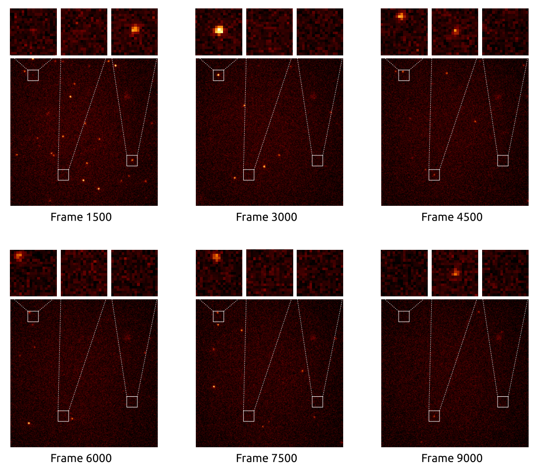
Quantitative biology addresses the issue of counting the number of fluorophores from measurements like the one described above. The brightness of each spot is proportional to the number of fluorophores in the active state within the respective origami. Thus, an origami is invisible if all of its fluorophores are inactive, but its location on the image is still known from the first frame. This allows us to register 94 regions of interest (ROIs) marked in Figure 1(b). For illustration, six microscopic frames recorded at the times tโˆˆ{1500,3000,4500,6000,7500,9000}t\in\{1500,3000,4500,6000,7500,9000\} are visualized in Figure 4.2. The influence of switching and bleaching on the observations is clearly visible.

We aim to estimate the number of fluorophores attached to each origami, which is expected to be between 1313 and 1717. For simplicity, we assume that each origami carries the same number n0n_{0} of fluorophores and we only model the mean number ntn_{t} of unbleached fluorophores at time tt. The physical relation between n0n_{0} and ntn_{t} is given by

nt=n0โ€‹(1โˆ’pb)t,n_{t}=n_{0}\,(1-p_{\mathrm{b}})^{t}, (4.1)

where pbp_{\mathrm{b}} denotes the bleaching probability. The brightness observed for a spot in frame tt is proportional to the (random) number XtX_{t} of active fluorophores during the frameโ€™s exposure. This number is binomially distributed, XtโˆผBinโก(nt,p)X_{t}\sim\mathrm{Bin}(n_{t},p), where pp denotes the (time-independent) probability that an unbleached fluorophore is in its active state. We will estimate n0n_{0} and pbp_{\mathrm{b}} by fitting a log-linear model to equation (4.1), where the respective population sizes ntn_{t} are in turn estimated from the 94 realizations of XtX_{t} observed in frame tt.

Refer to caption
Figure 4.2: Six selected frames from the data set of recorded origami. The (physical) time difference between two consecutive images in this figure is roughly 23 seconds. Bleaching causes the number of visible origami to decrease with increasing frame number, while switching causes that unbleached origami are visible only in some frames.

To get a sense for the magnitude of pp, we use prior information from a similar experiment where each origami has been designed to carry exactly one fluorophore. We calculate the average ratio between the number of frames where the fluorophore is active (a bright spot is seen) and the total number of frames before bleaching, which yields p~โ‰ˆ0.0339\tilde{p}\approx 0.0339 as a prior guess for pp. Therefore, we are indeed in the difficult small-pp regime of the binomial (n,p)(n,p) problem and will estimate ntn_{t} via the Bayesian scale estimators (1.2), using the notation (SE, PME) of Section 3. The beta prior for SE and PME uses the parameters a=2a=2 and b=2/p~โˆ’2โ‰ˆ56.99b=2/\tilde{p}-2\approx 56.99. We choose the unimodal prior with a=2a=2, as suggested by Table 2, since we assume that our guess p~\tilde{p} is reasonably accurate. Note that a finer degree of modeling would require to view n0n_{0}, ntn_{t} and pp as random variables instead of constants. However, as shown at the end of Section 3, the Bayesian estimators we consider are robust against fluctuations in the parameters and are therefore suited to estimate the respective mean values.

Since most fluorophores are deliberately forced to be active in the first frame, the relation XtโˆผBinโก(nt,p)X_{t}\sim\mathrm{Bin}(n_{t},p) does not hold initially. It only becomes valid after the initial state has relaxed to an equilibrium, which is why we only take into account data after frame 1500, about 2323 seconds into the experiment. To mitigate the influence of correlations between observations (since XtX_{t} and Xt+1X_{t+1} for a spot can not be considered independent), we also add a waiting time of 15001500 frames between the frames we use for our analysis. In total, we use the six frames at tโˆˆ{1500,3000,4500,6000,7500,9000}t\in\{1500,3000,4500,6000,7500,9000\} depicted in Figure 4.2. The 94 realizations of XtX_{t} are extracted from the image data as follows: at each registered origami position, represented by a 6ร—66\times 6 pixel ROI, the total brightness is measured and then divided by the brightness of a single fluorophore. We determined the brightness of a single fluorophore from the late frames of the experiment, where typically at most one fluorophore of each origami is active.

estimator n0n_{0} pbโ‹…103p_{\mathrm{b}}\cdot 10^{3}
SE(0)(0) 16 0.152
SE(0.5)(0.5) 13 0.148
SE(1)(1) 11 0.139
SE(2)(2) 9 0.163
SE(3)(3) 6 0.123
SE(5)(5) 5 0.114
PME(0)(0) 16 0.167
Table 5: Estimates of the bleaching probability pbp_{\mathrm{b}} and the number n0n_{0} of fluorophore molecules on single DNA origami.

The results for the scale estimator SEโก(0.5)\mathrm{SE}(0.5) are depicted in Figure 3(a), which shows the log-linear fit for model (4.1). The point estimates of n0n_{0} and pbp_{\mathrm{b}} for different estimators are summarized in Table 5. Given that the true n0n_{0} in this experiment is expected to be between 13 and 17, we can see that the scale estimators with an improper prior (ฮณโ‰ค1\gamma\leq 1) produce the most reasonable results. This is in agreement with our observations in Section 3, where we noted that priors putting a lot of weight on large values of nn perform better for small pp by correcting for the inherent tendency to underestimate (see Table 2). To illustrate the difficulty of this problem, Figure 3(b) shows exemplary counting results for tโˆˆ{1500,7500}t\in\{1500,7500\}. Note that estimates for each ntn_{t} are exclusively based on observations Xtโ‰ค3X_{t}\leq 3, where a great majority is even zero.

(a)
Refer to caption
(b)
Figure 4.3: (a) Log-linear fit described by nt=n0โ€‹(1โˆ’pb)tn_{t}=n_{0}\,(1-p_{\mathrm{b}})^{t} for the SE with ฮณ=0.5\gamma=0.5. (b) Bar charts of the observed numbers of fluorophore molecules for time frames 1500 and 7500.

5 Proofs and Auxiliary Results

In the following, we prove the posterior contraction result of Theorem 1, beginning by an outline of the main ideas.

Outline and comments

Throughout the proof, we fix some ฮป>1\lambda>1 and consider a generic sequence (nk,pk)k(n_{k},p_{k})_{k} of parameters that satisfies (nk,pk)โˆˆโ„ณkโ€‹(ฮป)(n_{k},p_{k})\in\mathcal{M}_{k}(\lambda) for all kโˆˆโ„•k\in\mathbb{N} with โ„ณkโ€‹(ฮป)\mathcal{M}_{k}(\lambda) as defined in (1.4). Since the convergence in Theorem 1 is uniform over โ„ณkโ€‹(ฮป)\mathcal{M}_{k}(\lambda), we emphasize that our arguments are indeed independent of the specific choice of (nk,pk)k(n_{k},p_{k})_{k} and all bounds are controlled by the parameter ฮป\lambda alone. For brevity, we usually write โ„™k\mathbb{P}_{k} and ๐”ผk\mathbb{E}_{k} instead of โ„™nk,pk\mathbb{P}_{n_{k},p_{k}} and ๐”ผnk,pk\mathbb{E}_{n_{k},p_{k}} from now on.

Let AkโŠ‚โ„•A_{k}\subset\mathbb{N} be a series of sets that do not contain the true parameter value nkn_{k}. The first step of the proof consists of bounding the (marginal) posterior probability ฮ โก(nโˆˆAk|๐—k)\Pi(n\in A_{k}\,|\,\mathbf{X}^{k}) in terms of fractions La,bโ€‹(n)/La,bโ€‹(nk)L_{a,b}(n)/L_{a,b}(n_{k}) of beta-binomial likelihoods (defined in (2.1)) for integers nโˆˆAkn\in A_{k}. Recall that MkM_{k} denotes the sample maximum and Sk=โˆ‘i=1kXiS_{k}=\sum_{i=1}^{k}X_{i} the sample sum. Consider the function R:[0,โˆž)ร—(0,โˆž)ร—[Mk,โˆž)โ†’(0,โˆž)R:[0,\infty)\times(0,\infty)\times[M_{k},\infty)\to(0,\infty),

Rโก(a,b,m)=โˆi=1kฮ“โก(m+1)ฮ“โก(Xi+1)โ€‹ฮ“โ€‹(mโˆ’Xi+1)โ€‹ฮ“โก(kโ€‹mโˆ’Sk+b)โ€‹ฮ“โ€‹(Sk+a)ฮ“โก(kโ€‹m+a+b),R(a,b,m)=\prod_{i=1}^{k}\frac{\Gamma(m+1)}{\Gamma(X_{i}+1)\,\Gamma(m-X_{i}+1)}\,\frac{\Gamma(km-S_{k}+b)\,\Gamma(S_{k}+a)}{\Gamma(km+a+b)}, (5.1)

which is well defined (even for a=0a=0) if Sk>0S_{k}>0. In particular, note that Rโก(a,b,n)=La,bโ€‹(n)R(a,b,n)=L_{a,b}(n) for a,bโˆˆ(0,โˆž)a,b\in(0,\infty) and nโ‰ฅMkn\geq M_{k}, so that one can write

Rโก(a,b,n)Rโก(a,b,nk)=expโก(kโ€‹โˆซnknfโ€ฒโ€‹(m)โ€‹๐‘‘m),\frac{R(a,b,n)}{R(a,b,n_{k})}=\exp\left(k\,\int_{n_{k}}^{n}f^{\prime}(m)\,\mathrm{d}m\right), (5.2)

where fโก(m):=1kโ€‹logโกRโก(a,b,m)f(m):=\frac{1}{k}\log R(a,b,m) is differentiable. The derivative fโ€ฒโ€‹(m)f^{\prime}(m) is studied in Hall (1994).

The remainder of the proof focuses on bounding fโ€ฒโ€‹(m)f^{\prime}(m). This includes the definition of an event ๐’ณk\mathcal{X}_{k} that satisfies โ„™โก(๐’ณk)โ†’1\mathbb{P}(\mathcal{X}_{k})\to 1 for kโ†’โˆžk\to\infty. We construct this event in such a way that MkM_{k}, SkS_{k}, and the factorial moments (Xi)j(X_{i})_{j}, where (c)j:=cโ‹…(cโˆ’1)โ‹ฏ(cโˆ’j+1)(c)_{j}:=c\cdot(c-1)\cdots(c-j+1) for cโˆˆโ„c\in\mathbb{R} and jโˆˆโ„•j\in\mathbb{N}, exhibit benign properties if ๐—kโˆˆ๐’ณk\mathbf{X}^{k}\in\mathcal{X}_{k}. We also need to distinguish between the cases mโ‰คnkm\leq n_{k} and m>nkm>n_{k}, for which we have to lower-, respectively upper-bound fโ€ฒโ€‹(m)f^{\prime}(m) on ๐’ณk\mathcal{X}_{k}. This requires several technical interim steps, which are largely outsourced to Section A in the supplement. Combining the resulting bounds yields an upper bound for ฮ โก(nโˆˆAk|๐—k)\Pi\big(n\in A_{k}\,\big|\,\mathbf{X}^{k}\big) that can be used to show consistency in the asymptotic setting explored in Theorem 1 if the sets AkA_{k} are chosen suitably.

Let AkโŠ‚โ„•A_{k}\subset\mathbb{N} be sets such that nkโˆ‰Akn_{k}\not\in A_{k} for all kk. It will later become evident how these sets are best be chosen. First observe that

ฮ โก(nโˆˆAk|๐—k)=โˆ‘nโˆˆAk,nโ‰ฅMkLa,bโ€‹(n)โ€‹ฮ nโ€‹(n)โˆ‘n=MkโˆžLa,bโ€‹(n)โ€‹ฮ nโ€‹(n)โ‰คโˆ‘nโˆˆAk,nโ‰ฅMkLa,bโ€‹(n)โ€‹ฮ nโ€‹(n)La,bโ€‹(nk)โ€‹ฮ nโ€‹(nk).\Pi\big(n\in A_{k}\,|\,\mathbf{X}^{k}\big)=\frac{\sum_{n\in A_{k},n\geq M_{k}}\!L_{a,b}(n)\,\Pi_{n}(n)}{\sum_{n=M_{k}}^{\infty}L_{a,b}(n)\,\Pi_{n}(n)}\leq\!\!\!\sum_{n\in A_{k},n\geq M_{k}}\!\frac{L_{a,b}(n)\,\Pi_{n}(n)}{L_{a,b}(n_{k})\,\Pi_{n}(n_{k})}.

Under the assumption that Skโ‰ฅ2S_{k}\geq 2, which we justify below, we can apply Lemma 4 and find

La,bโ€‹(n)La,bโ€‹(nk)โ‰คRโก(โŒŠaโŒ‹,b,n)Rโก(โŒˆaโŒ‰,b,nk)โ‰คc1โ€‹kโ€‹nkSkโ€‹Rโก(โŒŠaโŒ‹,b,n)Rโก(โŒŠaโŒ‹,b,nk)\frac{L_{a,b}(n)}{L_{a,b}(n_{k})}\leq\frac{R(\lfloor a\rfloor,b,n)}{R(\lceil a\rceil,b,n_{k})}\leq c_{1}\frac{kn_{k}}{S_{k}}\,\frac{R(\lfloor a\rfloor,b,n)}{R(\lfloor a\rfloor,b,n_{k})}

for c1=2โ€‹(1+โŒˆaโŒ‰+b)c_{1}=2\,(1+\lceil a\rceil+b), where โŒˆโ‹…โŒ‰\lceil\cdot\rceil and โŒŠโ‹…โŒ‹\lfloor\cdot\rfloor denote the ceiling and floor functions, and where RR was defined in (5.1). It follows that

ฮ โก(nโˆˆAk|๐—k)โ‰คc1โ€‹kโ€‹nkSkโ€‹โˆ‘nโˆˆAk,nโ‰ฅMkexpโก(kโ€‹โˆซnknfโ€ฒโ€‹(m)โ€‹๐‘‘m)โ€‹ฮ nโ€‹(n)ฮ nโ€‹(nk),\Pi\big(n\in A_{k}\,|\,\mathbf{X}^{k}\big)\leq c_{1}\frac{kn_{k}}{S_{k}}\,\sum_{n\in A_{k},n\geq M_{k}}\exp\left(k\int_{n_{k}}^{n}f^{\prime}(m)\,\mathrm{d}m\right)\,\frac{\Pi_{n}(n)}{\Pi_{n}(n_{k})}, (5.3)

where fโก(m)=1kโ€‹logโกRโก(โŒŠaโŒ‹,b,m)f(m)=\frac{1}{k}\log R(\lfloor a\rfloor,b,m). In case that n<nkn<n_{k}, we find โˆซnknfโ€ฒ(m)dm=โˆ’โˆซnnkfโ€ฒ(m)dm\int_{n_{k}}^{n}f^{\prime}(m)\,\mathrm{d}m=-\int_{n}^{n_{k}}f^{\prime}(m)\,\mathrm{d}m. For an upper bound on the posterior we thus need a lower bound of fโ€ฒโ€‹(m)f^{\prime}(m) if Mkโ‰คmโ‰คnkM_{k}\leq m\leq n_{k} and an upper bound if mโ‰ฅnkm\geq n_{k}. Since ff only depends on aa via โŒŠaโŒ‹\lfloor a\rfloor, we for brevity write aโˆˆโ„•0a\in\mathbb{N}_{0} to denote โŒŠaโŒ‹\lfloor a\rfloor from now on. Lemma 4.1 in Hall (1994) states that

โˆ‘j=1r1cโˆ’j+1=โˆ‘j=1r(r)j(cj)jโ€‹j\sum_{j=1}^{r}\frac{1}{c-j+1}=\sum_{j=1}^{r}\frac{(r)_{j}}{(c_{j})_{j}j}

for integers rโˆˆโ„•r\in\mathbb{N} and positive numbers c>kโˆ’1c>k-1. We therefore find

fโ€ฒโ€‹(m)=1kโ€‹โˆ‘i=1kโˆ‘j=1Xi1mโˆ’j+1โˆ’โˆ‘j=1Sk+a1kโ€‹m+a+bโˆ’j=โˆ‘j=1MkTjโˆ’Ujjโˆ’โˆ‘j=Mk+1Sk+aUjj\begin{split}f^{\prime}(m)&=\frac{1}{k}\sum_{i=1}^{k}\sum_{j=1}^{X_{i}}\frac{1}{m-j+1}-\sum_{j=1}^{S_{k}+a}\frac{1}{km+a+b-j}\\ &=\sum_{j=1}^{M_{k}}\frac{T_{j}-U_{j}}{j}-\sum_{j=M_{k}+1}^{S_{k}+a}\frac{U_{j}}{j}\end{split} (5.4)

with

Tj:=1kโ€‹โˆ‘i=1k(Xi)j(m)jandUj:=(Sk+a)j(kโ€‹m+a+bโˆ’1)jT_{j}:=\frac{1}{k}\sum_{i=1}^{k}\frac{(X_{i})_{j}}{(m)_{j}}\qquad\text{and}\qquad U_{j}:=\frac{(S_{k}+a)_{j}}{(km+a+b-1)_{j}} (5.5)

for jโ‰คMkj\leq M_{k} and jโ‰คSk+aj\leq S_{k}+a respectively. If j>Mkj>M_{k}, we define Tj:=0T_{j}:=0 for all j>Mkj>M_{k}. The expectation of TjT_{j} is given by tj:=๐”ผkโ€‹[Tj]=(nk)jโ€‹(pk)j/(m)jt_{j}:=\mathbb{E}_{k}[T_{j}]=(n_{k})_{j}(p_{k})^{j}/(m)_{j}, which follows from

๐”ผkโ€‹[(Xi)j]=โˆ‘x=jnk(nkx)โ€‹(x)jโ€‹pkxโ€‹qknkโˆ’x=(nk)jโ€‹(pk)jโ€‹โˆ‘y=0nkโˆ’j(nkโˆ’jy)โ€‹pkyโ€‹qknkโˆ’jโˆ’yโŸ=โ€‰1\mathbb{E}_{k}[(X_{i})_{j}]=\sum_{x=j}^{n_{k}}\binom{n_{k}}{x}(x)_{j}\,p_{k}^{x}q_{k}^{n_{k}-x}=(n_{k})_{j}(p_{k})^{j}\,\underbrace{\sum_{y=0}^{n_{k}-j}\binom{n_{k}-j}{y}\,p_{k}^{y}q_{k}^{n_{k}-j-y}}_{=\,1}

for all i=1,โ€ฆ,ki=1,\ldots,k, where we set qk:=1โˆ’pkq_{k}:=1-p_{k} and substituted y=xโˆ’jy=x-j.

Next, recall that ฮป>1\lambda>1 is the constant in the definition of the spaces โ„ณkโ€‹(ฮป).\mathcal{M}_{k}(\lambda). For a fixed positive and diverging sequence lk=oโก(logโก(k))l_{k}=o\big(\sqrt{\log(k)}\big) and c2=2โ€‹ฮปโ€‹(ฮป+1)c_{2}=2\,\lambda\,(\lambda+1), we introduce the events

โ„›k:={min(nk,lk)โ‰คMkโ‰ค2log(k)},๐’ฏk:=โ‹‚j=1Mk{(m)j|Tjโˆ’tj|โ‰ค(c2โ€‹j)jโ€‹lkโ€‹logโก(k)/k},๐’ฎk:={|Skโˆ’knkpk|โ‰คฮปโ€‹kโ€‹logโก(k)},\displaystyle\begin{split}\mathcal{R}_{k}&:=\big\{\min(n_{k},l_{k})\leq M_{k}\leq 2\log(k)\big\},\\[2.84544pt] \mathcal{T}_{k}&:=\bigcap_{j=1}^{M_{k}}\Big\{(m)_{j}\,\big|\,T_{j}-t_{j}\big|\leq\sqrt{(c_{2}j)^{j}\,l_{k}\log(k)/k}\,\Big\},\\[2.84544pt] \mathcal{S}_{k}&:=\Big\{\big|S_{k}-kn_{k}p_{k}\big|\leq\sqrt{\lambda\,k\log(k)}\Big\},\end{split} (5.6)

and denote their intersection โ„›kโˆฉ๐’ฏkโˆฉ๐’ฎk\,\mathcal{R}_{k}\,\cap\,\mathcal{T}_{k}\,\cap\,\mathcal{S}_{k}\, by ๐’ณk\mathcal{X}_{k}. The probability of the event ๐’ฏk\mathcal{T}_{k} is independent of mm due to the definition of TjT_{j}. On the event ๐’ฎk\mathcal{S}_{k}, Lemma 6 grants us the additional property

|Ujโˆ’uj|โ‰คjโ€‹ฮปโ€‹logโก(k)kโ€‹(c3m)jwithuj:=(kโ€‹nkโ€‹pk+a)j(kโ€‹m+a+bโˆ’1)j\big|U_{j}-u_{j}\big|\leq j\,\sqrt{\frac{\lambda\log(k)}{k}}\left(\frac{c_{3}}{m}\right)^{j}\qquad\text{with}\qquad u_{j}:=\frac{(kn_{k}p_{k}+a)_{j}}{(km+a+b-1)_{j}}

for jโ‰คSk+aj\leq S_{k}+a and c3=2โ€‹e2โ€‹(3โ€‹ฮป+a+1)c_{3}=2e^{2}(3\lambda+a+1). If k/logโก(k)โ‰ฅ4โ€‹ฮป3k/\log(k)\geq 4\lambda^{3}, then k/2โ€‹ฮปโ‰คSkโ‰ค2โ€‹ฮปโ€‹kk/2\lambda\leq S_{k}\leq 2\lambda k and Skโ‰ฅ2S_{k}\geq 2 on ๐’ฎk\mathcal{S}_{k}. Hence, equations (5.3) and (5.4) apply on ๐’ณk\mathcal{X}_{k} if kk is sufficiently large. Also, we can use

c1โ€‹kโ€‹nk/Skโ‰ค2โ€‹ฮปโ€‹c1โ€‹nkc_{1}kn_{k}/S_{k}\leq 2\lambda c_{1}\,n_{k} (5.7)

to bound the factor preceding the sum in (5.3).

For the remainder of the proof, we can restrict ๐—k\mathbf{X}^{k} to ๐’ณk\mathcal{X}_{k} since

๐”ผkโ€‹[ฮ โก(nโ‰ nk|๐—k)]โˆ’๐”ผkโ€‹[๐Ÿ๐’ณkโ€‹ฮ โ€‹(nโ‰ nk|๐—k)]โ‰คโ„™kโ€‹(๐’ณkc)โŸถ0\mathbb{E}_{k}\big[\Pi\big(n\neq n_{k}\,|\,\mathbf{X}^{k}\big)\big]-\mathbb{E}_{k}\big[\mathbf{1}_{\mathcal{X}_{k}}\Pi\big(n\neq n_{k}\,|\,\mathbf{X}^{k}\big)\big]\leq\mathbb{P}_{k}\big(\mathcal{X}_{k}^{\mathrm{c}}\big)\longrightarrow 0 (5.8)

uniformly over โ„ณkโ€‹(ฮป)\mathcal{M}_{k}(\lambda) for kโ†’โˆžk\to\infty. To show this, we bound

โ„™kโ€‹(๐’ณkc)โ‰คโ„™kโ€‹(๐’ฎkc)+2โ€‹โ„™kโ€‹(โ„›kc)+โ„™kโ€‹(๐’ฏkcโˆฉโ„›k).\mathbb{P}_{k}\big(\mathcal{X}_{k}^{\mathrm{c}}\big)\leq\mathbb{P}_{k}\big(\mathcal{S}_{k}^{\mathrm{c}}\big)+2\,\mathbb{P}_{k}\big(\mathcal{R}_{k}^{\mathrm{c}}\big)+\mathbb{P}_{k}\big(\mathcal{T}_{k}^{\mathrm{c}}\cap\mathcal{R}_{k}\big).

The first contribution vanishes by the application of Chebyshevโ€™s inequality (see, e.g., DeGroot and Schervish (2012)), because ๐”ผkโ€‹[Sk]=kโ€‹nkโ€‹pk\mathbb{E}_{k}[S_{k}]=kn_{k}p_{k} and Varkโก[Sk]=kโ€‹nkโ€‹pkโ€‹(1โˆ’pk)โ‰คkโ€‹ฮป\operatorname{Var}_{k}[S_{k}]=kn_{k}p_{k}(1-p_{k})\leq k\lambda. The second term is controlled by Lemma 2. For the last term, observe that

Varโก[(Xi)j]โ‰ค(2โ€‹jโ€‹nโ€‹pโ€‹(nโ€‹p+1))jโ‰ค(2โ€‹jโ€‹ฮปโ€‹(ฮป+1))j=(c2โ€‹j)j\mathrm{Var}[(X_{i})_{j}]\leq(2j\,np\,(np+1))^{j}\leq(2j\,\lambda\,(\lambda+1))^{j}=(c_{2}j)^{j}

by Lemma 1. For any r>0r>0, Chebyshevโ€™s inequality yields

โ„™k(|1kโ€‹โˆ‘i=1k(Xi)jโˆ’๐”ผโก[(X1)j]|>rโ€‹(c2โ€‹j)jkโŸ=:๐’ฏjโ€‹kcโ€‹(r))โ‰คVarโก[(X1)j]/krโ€‹(c2โ€‹j)j/kโ‰ค1r.\mathbb{P}_{k}\bigg(\underbrace{\bigg|\frac{1}{k}\sum_{i=1}^{k}(X_{i})_{j}-\mathbb{E}[(X_{1})_{j}]\bigg|>\sqrt{\frac{r\,(c_{2}j)^{j}}{k}}}_{=:\,\mathcal{T}_{jk}^{\mathrm{c}}(r)}\bigg)\leq\frac{\mathrm{Var}[(X_{1})_{j}]/k}{r\,(c_{2}j)^{j}/k}\leq\frac{1}{r}.

With r=lkโ€‹logโก(k)r=l_{k}\log(k) and Mkโ‰ค2โ€‹logโก(k)M_{k}\leq 2\log(k) on โ„›k\mathcal{R}_{k},

โ„™kโ€‹(๐’ฏkcโˆฉโ„›k)\displaystyle\mathbb{P}_{k}\big(\mathcal{T}_{k}^{\mathrm{c}}\cap\mathcal{R}_{k}\big) =โ„™kโ€‹(โ‹ƒ1โ‰คjโ‰ค2โ€‹logโก(k)๐’ฏjโ€‹kcโ€‹(lkโ€‹logโก(k)))โ‰ค2โ€‹logโก(k)lkโ€‹logโก(k)โŸถ0\displaystyle=\mathbb{P}_{k}\left(\bigcup\nolimits_{1\leq j\leq 2\log(k)}\mathcal{T}_{jk}^{\mathrm{c}}\big(l_{k}\log(k)\big)\right)\leq\frac{2\log(k)}{l_{k}\log(k)}\longrightarrow 0

follows. It is important to note that the upper bounds in these inequalities are all controlled by ฮป\lambda, which implies that the convergence in (5.8) is indeed uniform over โ„ณkโ€‹(ฮป)\mathcal{M}_{k}(\lambda).

Auxiliary lower bound

For Mkโ‰คm<nkM_{k}\leq m<n_{k}, we prove a lower bound for fโ€ฒโ€‹(m)f^{\prime}(m). We may assume that Mkโ‰ฅlkโ†’โˆžM_{k}\geq l_{k}\to\infty for kโ†’โˆžk\to\infty in this case, since ๐—kโˆˆโ„›k\mathbf{X}^{k}\in\mathcal{R}_{k}. For kk such that lkโ‰ฅ4,l_{k}\geq 4, equation (5.4) yields

fโ€ฒโ€‹(m)โ‰ฅโˆ‘j=14Tjโˆ’Ujjโˆ’โˆ‘5Sk+aUjj,f^{\prime}(m)\geq\sum_{j=1}^{4}\frac{T_{j}-U_{j}}{j}-\sum_{5}^{S_{k}+a}\frac{U_{j}}{j}, (5.9)

as Tjโ‰ฅ0T_{j}\geq 0 for all jj. Due to the definition of โ„ณkโ€‹(ฮป),\mathcal{M}_{k}(\lambda), we can (generously) bound m<nkโ‰คฮปโ€‹kโ€‹logโก(k)m<n_{k}\leq\lambda\sqrt{k\log(k)} and

T1โˆ’U1=Skkโ€‹mโˆ’Sk+akโ€‹m+a+bโˆ’1โ‰ฅโˆ’a+1kโ€‹mโˆ’1โ‰ฅโˆ’2โ€‹ฮปโก(a+1)m2โ€‹logโก(k)k.T_{1}-U_{1}=\frac{S_{k}}{km}-\frac{S_{k}+a}{km+a+b-1}\geq-\frac{a+1}{km-1}\geq-2\,\frac{\lambda(a+1)}{m^{2}}\sqrt{\frac{\log(k)}{k}}.

To handle the terms in (5.9) with jโ‰ฅ2j\geq 2, we exploit that ๐—kโˆˆ๐’ฏk\mathbf{X}^{k}\in\mathcal{T}_{k} and apply (m)jโ‰ฅ(m/e2)j(m)_{j}\geq\big(m/e^{2}\big)^{j} (see Lemma 5) in order to derive

โˆ‘j=24|Tjโˆ’tj|jโ‰คlkโ€‹logโก(k)kโ€‹โˆ‘j=24(c2โ€‹jm/e2)jโ‰ค2โ€‹4โ€‹c2โ€‹e4m2โ€‹lkโ€‹logโก(k)k\sum_{j=2}^{4}\frac{\big|T_{j}-t_{j}\big|}{j}\leq\sqrt{\frac{l_{k}\log(k)}{k}}\penalty\ \sum_{j=2}^{4}\left(\frac{\sqrt{c_{2}j}}{m/e^{2}}\right)^{j}\leq 2\,\frac{4\,c_{2}\,e^{4}}{m^{2}}\penalty\ \sqrt{\frac{l_{k}\log(k)}{k}}

for sufficiently large kk such that 4โ€‹c2โ€‹e2/lk<1/2\sqrt{4\,c_{2}}\,e^{2}/l_{k}<1/2. Similarly, we find

โˆ‘j=2Sk+a|Ujโˆ’uj|jโ‰คฮปโ€‹logโก(k)kโ€‹โˆ‘j=2Sk+a(c3m)jโ‰ค2โ€‹ฮปโ€‹c32m2โ€‹logโก(k)k\sum_{j=2}^{S_{k}+a}\frac{\big|U_{j}-u_{j}\big|}{j}\leq\sqrt{\frac{\lambda\log(k)}{k}}\penalty\ \sum_{j=2}^{S_{k}+a}\left(\frac{c_{3}}{m}\right)^{j}\leq 2\,\frac{\sqrt{\lambda}\,c_{3}^{2}}{m^{2}}\penalty\ \sqrt{\frac{\log(k)}{k}}

for mโ‰ฅlkโ‰ฅ2โ€‹c3m\geq l_{k}\geq 2c_{3}. By applying Lemma 7 with c4=6โ€‹e2โ€‹(ฮป+a)c_{4}=6e^{2}(\lambda+a) and using Skโ‰ค2โ€‹kโ€‹ฮปS_{k}\leq 2\,k\lambda on ๐’ฎk,\mathcal{S}_{k}, we furthermore observe

โˆ‘j=5Sk+aujjโ‰คโˆ‘j=5Sk+a1jโ€‹(c4m)jโ‰ค2โ€‹(c4m)5\sum_{j=5}^{S_{k}+a}\frac{u_{j}}{j}\leq\sum_{j=5}^{S_{k}+a}\frac{1}{j}\left(\frac{c_{4}}{m}\right)^{j}\leq 2\,\left(\frac{c_{4}}{m}\right)^{5}

for all kk (and thus mm) that are sufficiently large. The first result of Lemma 8 combined with m<nkโ‰คฮปโ€‹kโ€‹logโก(k)m<n_{k}\leq\lambda\sqrt{k\log(k)} reveals

โˆ‘j=24tjโˆ’ujjโ‰ฅ12โ€‹ฮป2โ€‹nkโˆ’mnkโ€‹m3โˆ’3โ€‹c54mโ€‹kโ‰ฅ12โ€‹ฮป2โ€‹nkโˆ’mnkโ€‹m3โˆ’2โ€‹2โ€‹ฮปโ€‹c54m2โ€‹logโก(k)k,\sum_{j=2}^{4}\frac{t_{j}-u_{j}}{j}\geq\frac{1}{2\lambda^{2}}\frac{n_{k}-m}{n_{k}m^{3}}-\frac{3\,c_{5}^{4}}{mk}\geq\frac{1}{2\lambda^{2}}\frac{n_{k}-m}{n_{k}m^{3}}-2\,\frac{2\,\lambda\,c_{5}^{4}}{m^{2}}\sqrt{\frac{\log(k)}{k}},

where c5=3โ€‹ฮปโ€‹(1+a+b)+2โ€‹a+4c_{5}=3\,\lambda(1+a+b)+2\,a+4. All bounds calculated above can be inserted into inequality (5.9), yielding

fโ€ฒโ€‹(m)\displaystyle f^{\prime}(m) โ‰ฅ(T1โˆ’U1)+โˆ‘j=24Tjโˆ’tjj+โˆ‘j=2Sk+aujโˆ’Ujj+โˆ‘j=24tjโˆ’ujjโˆ’โˆ‘j=5Sk+aujj\displaystyle\geq(T_{1}-U_{1})+\sum_{j=2}^{4}\frac{T_{j}-t_{j}}{j}+\sum_{j=2}^{S_{k}+a}\frac{u_{j}-U_{j}}{j}+\sum_{j=2}^{4}\frac{t_{j}-u_{j}}{j}-\sum_{j=5}^{S_{k}+a}\frac{u_{j}}{j}
โ‰ฅC1nkโˆ’mnkโ€‹m3โˆ’C2m2lkโ€‹logโก(k)k+[14โ€‹ฮป2โ€‹nkโˆ’mnkโ€‹m3โˆ’2โ€‹(c4m)5]โŸ=:hโก(m)\displaystyle\geq C_{1}\frac{n_{k}-m}{n_{k}m^{3}}-\frac{C_{2}}{m^{2}}\,\sqrt{\frac{l_{k}\log(k)}{k}}+\underbrace{\left[\frac{1}{4\lambda^{2}}\frac{n_{k}-m}{n_{k}m^{3}}-2\,\left(\frac{c_{4}}{m}\right)^{5}\right]}_{=:\,h(m)} (5.10)

with C1=1/(4โ€‹ฮป2)C_{1}=1/(4\lambda^{2}) and C2=2โ€‹(ฮปโก(a+1)+4โ€‹c2โ€‹e4+ฮปโ€‹c32+2โ€‹ฮปโ€‹c54)C_{2}=2\,\big(\lambda(a+1)+4\,c_{2}\,e^{4}+\sqrt{\lambda}\,c_{3}^{2}+2\,\lambda\,c_{5}^{4}\big).

Auxiliary upper bound

We next provide an upper bound for fโ€ฒโ€‹(m)f^{\prime}(m) for m>nkโ‰ฅMkm>n_{k}\geq M_{k}. Unlike for the lower bound, we can not assume that mm becomes larger than any given constant with increasing kk as nkn_{k} could stay bounded. Since UjU_{j} is nonnegative, we can derive

fโ€ฒโ€‹(m)โ‰คโˆ‘j=1MkTjโˆ’Ujjf^{\prime}(m)\leq\sum_{j=1}^{M_{k}}\frac{T_{j}-U_{j}}{j}

from equation (5.4). For j=1,j=1,

T1โˆ’U1=Skkโ€‹mโˆ’Sk+akโ€‹m+a+bโˆ’1โ‰คSkโ€‹(a+b)kโ€‹mโ€‹(kโ€‹mโˆ’1)โ‰ค4โ€‹ฮปโ€‹(a+b)m2โ€‹log3โก(k)k,T_{1}-U_{1}=\frac{S_{k}}{km}-\frac{S_{k}+a}{km+a+b-1}\leq\frac{S_{k}\,(a+b)}{km\,(km-1)}\leq\frac{4\lambda\,(a+b)}{m^{2}}\sqrt{\frac{\log^{3}(k)}{k}},

where we used that Skโ‰ค2โ€‹ฮปโ€‹kS_{k}\leq 2\lambda\,k on the event ๐’ฎk\mathcal{S}_{k}. Next we set m0:=4โ€‹c2โ€‹e4m_{0}:=4\,c_{2}\,e^{4} and derive

โˆ‘j=2Mk|Tjโˆ’tj|j\displaystyle\sum_{j=2}^{M_{k}}\frac{\big|T_{j}-t_{j}\big|}{j} โ‰คlkโ€‹logโก(k)kโ€‹โˆ‘j=2Mk(c2โ€‹jm/e2)j\displaystyle\leq\sqrt{\frac{l_{k}\log(k)}{k}}\penalty\ \sum_{j=2}^{M_{k}}\left(\frac{\sqrt{c_{2}j}}{m/e^{2}}\right)^{j}
โ‰คc2โ€‹Mkโ€‹e4m2โ€‹lkโ€‹logโก(k)kโ€‹โˆ‘j=0โŒŠmโŒ‹(e2โ€‹c2m)j\displaystyle\leq\frac{c_{2}M_{k}\,e^{4}}{m^{2}}\penalty\ \sqrt{\frac{l_{k}\log(k)}{k}}\penalty\ \sum_{j=0}^{\lfloor m\rfloor}\left(\frac{e^{2}\sqrt{c_{2}}}{\sqrt{m}}\right)^{j}
โ‰คc2โ€‹Mkโ€‹e4m2โ€‹lkโ€‹logโก(k)kโ‹…{2ifโ€‹m>m0m0โ€‹(e2โ€‹c2+1)m0ifโ€‹mโ‰คm0\displaystyle\leq\frac{c_{2}M_{k}\,e^{4}}{m^{2}}\penalty\ \sqrt{\frac{l_{k}\log(k)}{k}}\cdot\begin{cases}2&\text{if}\penalty\ m>m_{0}\\ m_{0}\,(e^{2}\sqrt{c_{2}}+1)^{m_{0}}&\text{if}\penalty\ m\leq m_{0}\end{cases}
โ‰คc6m2โ€‹lkโ€‹log3โ€‹(k)k\displaystyle\leq\frac{c_{6}}{m^{2}}\penalty\ \sqrt{\frac{l_{k}\log^{3}(k)}{k}}

for c6=2โ€‹c2โ€‹e4โ€‹(m0โ€‹(e2โ€‹c2+1)m0+2)c_{6}=2\,c_{2}\,e^{4}\big(m_{0}\,(e^{2}\sqrt{c_{2}}+1)^{m_{0}}+2\big). In the last step, we used that Mkโ‰ค2โ€‹logโก(k)M_{k}\leq 2\log(k) on the event โ„›k\mathcal{R}_{k}. In a similar fashion, we can establish the bound

โˆ‘j=2Mk|Ujโˆ’uj|jโ‰คฮปโ€‹logโก(k)kโ€‹โˆ‘j=2Mk(c3m)jโ‰คc7m2โ€‹log3โก(k)k,\sum_{j=2}^{M_{k}}\frac{\big|U_{j}-u_{j}\big|}{j}\leq\sqrt{\frac{\lambda\log(k)}{k}}\penalty\ \sum_{j=2}^{M_{k}}\left(\frac{c_{3}}{m}\right)^{j}\leq\frac{c_{7}}{m^{2}}\penalty\ \sqrt{\frac{\log^{3}(k)}{k}},

where c7=4โ€‹ฮปโ€‹c32โ€‹(c32โ€‹c3+1+1)c_{7}=4\,\sqrt{\lambda}\,c_{3}^{2}\,\big(c_{3}^{2c_{3}+1}+1\big). Finally, we apply the second claim of Lemma 8 and obtain

โˆ‘j=2Mktjโˆ’ujjโ‰คโˆ’C1โ€ฒโ€‹mโˆ’nknkโ€‹m3+c8โ€‹logโก(k)m2โ€‹k\sum_{j=2}^{M_{k}}\frac{t_{j}-u_{j}}{j}\leq-C_{1}^{\prime}\,\frac{m-n_{k}}{n_{k}m^{3}}+c_{8}\frac{\log(k)}{m^{2}k}

with C1โ€ฒ=(ฮป2โ€‹(a+b+1)2)โˆ’1C_{1}^{\prime}=\big(\lambda^{2}\left(a+b+1\right)^{2}\big)^{-1} and c8=36โ€‹(1+ฮป)3โ€‹(1+a+b)2c_{8}=36(1+\lambda)^{3}(1+a+b)^{2} for sufficiently large kk. We conclude

fโ€ฒโ€‹(m)\displaystyle f^{\prime}(m) โ‰ค(T1โˆ’U1)+โˆ‘j=2MkTjโˆ’tjj+โˆ‘j=2Mkujโˆ’Ujj+โˆ‘j=2Mktjโˆ’ujj\displaystyle\leq(T_{1}-U_{1})+\sum_{j=2}^{M_{k}}\frac{T_{j}-t_{j}}{j}+\sum_{j=2}^{M_{k}}\frac{u_{j}-U_{j}}{j}+\sum_{j=2}^{M_{k}}\frac{t_{j}-u_{j}}{j}
โ‰คโˆ’C1โ€ฒm3โ€‹mโˆ’nknk+C2โ€ฒm2โ€‹lkโ€‹log3โ€‹(k)k\displaystyle\leq-\frac{C_{1}^{\prime}}{m^{3}}\frac{m-n_{k}}{n_{k}}+\frac{C_{2}^{\prime}}{m^{2}}\penalty\ \sqrt{\frac{l_{k}\,\log^{3}(k)}{k}} (5.11)

for C2โ€ฒ=4โ€‹ฮปโ€‹(a+b)+c6+c7+c8C_{2}^{\prime}=4\lambda\,(a+b)+c_{6}+c_{7}+c_{8}.

Posterior bound

By applying the two inequalities (5.10) and (5.11) for m<nkm<n_{k} and m>nkm>n_{k}, we can now bound the posterior probability ฮ โก(nโˆˆAk|๐—k)\Pi\big(n\in A_{k}\,|\,\mathbf{X}^{k}\big) on the event ๐’ณk\mathcal{X}_{k} through equation (5.3). Recall that we can assume nโ‰ nkn\neq n_{k} due to the assumption nkโˆ‰Akn_{k}\not\in A_{k}. We observe that

โˆซnknmโˆ’nknkโ€‹m3โ€‹๐‘‘m=12โ€‹(nโˆ’nk)2(nkโ€‹n)2andโˆซnkn1m2โ€‹๐‘‘m=12โ€‹(nโˆ’nk)2(nkโ€‹n)2โ€‹2โ€‹nkโ€‹nnโˆ’nk.\int_{n_{k}}^{n}\frac{m-n_{k}}{n_{k}m^{3}}\,\mathrm{d}m=\frac{1}{2}\frac{(n-n_{k})^{2}}{(n_{k}n)^{2}}\quad\penalty\ \penalty\ \text{and}\quad\penalty\ \penalty\ \int_{n_{k}}^{n}\frac{1}{m^{2}}\,\mathrm{d}m=\frac{1}{2}\frac{(n-n_{k})^{2}}{(n_{k}n)^{2}}\frac{2n_{k}n}{n-n_{k}}.

Noting |nโˆ’nk|โ‰ฅ1|n-n_{k}|\geq 1, it also holds that

|nnkโˆ’1|=|nโˆ’nk|nkโ‰ฅ{1/nkifโ€‹nkโ‰ค2โ€‹n1/2ifโ€‹nk>2โ€‹n}โ‰ฅ12โ€‹n.\left|\frac{n}{n_{k}}-1\right|=\frac{|n-n_{k}|}{n_{k}}\geq\left.\begin{cases}1/n_{k}&\text{if}\penalty\ n_{k}\leq 2n\\ 1/2&\text{if}\penalty\ n_{k}>2n\\ \end{cases}\right\}\geq\frac{1}{2n}\,. (5.12)

Therefore, if lkโ‰คn<nkl_{k}\leq n<n_{k}, the function hโก(m)h(m) introduced in equation (5.10) satisfies

โˆซnnkhโก(m)โ€‹๐‘‘m\displaystyle\int_{n}^{n_{k}}h(m)\,\mathrm{d}m =C12โ€‹(nโˆ’nk)2(nkโ€‹n)2โˆ’c452โ€‹nk4โˆ’n4(nkโ€‹n)4\displaystyle=\frac{C_{1}}{2}\,\frac{(n-n_{k})^{2}}{(n_{k}n)^{2}}-\frac{c_{4}^{5}}{2}\,\frac{n_{k}^{4}-n^{4}}{(n_{k}n)^{4}}
โ‰ฅC12โ€‹(nโˆ’nk)2(nkโ€‹n)2โ€‹(1โˆ’4โ€‹c45C1โ€‹11โˆ’n/nkโ€‹1n2)โ‰ฅ0\displaystyle\geq\frac{C_{1}}{2}\,\frac{(n-n_{k})^{2}}{(n_{k}n)^{2}}\left(1-\frac{4c_{4}^{5}}{C_{1}}\frac{1}{1-n/n_{k}}\frac{1}{n^{2}}\right)\geq 0 (5.13)

for kk such that lkโ‰ฅ8โ€‹c45/C1l_{k}\geq 8\,c_{4}^{5}/C_{1}. Employing bound (5.10) thus yields

โˆ’kโˆซnnkfโ€ฒ(m)dm\displaystyle-k\int_{n}^{n_{k}}f^{\prime}(m)\,\mathrm{d}m โ‰คโˆ’kโ€‹C12โ€‹(nโˆ’nk)2(nkโ€‹n)2โ€‹(1โˆ’Cโ€‹nkโ€‹nnkโˆ’nโ€‹lkโ€‹logโก(k)k),\displaystyle\leq-k\frac{C_{1}}{2}\frac{(n-n_{k})^{2}}{(n_{k}n)^{2}}\left(1-C\frac{n_{k}n}{n_{k}-n}\sqrt{\frac{l_{k}\log(k)}{k}}\right),
where the constant CC is given by 2โ€‹C2/C12\,C_{2}/C_{1}. On the other hand, for nk<nn_{k}<n, bound (5.11) similarly leads to
kโ€‹โˆซnknfโ€ฒโ€‹(m)โ€‹๐‘‘m\displaystyle k\int_{n_{k}}^{n}f^{\prime}(m)\,\mathrm{d}m โ‰คโˆ’kโ€‹C1โ€ฒ2โ€‹(nโˆ’nk)2(nkโ€‹n)2โ€‹(1โˆ’Cโ€ฒโ€‹nkโ€‹nnโˆ’nkโ€‹lkโ€‹log3โ€‹(k)k)\displaystyle\leq-k\frac{C_{1}^{\prime}}{2}\frac{(n-n_{k})^{2}}{(n_{k}n)^{2}}\left(1-C^{\prime}\frac{n_{k}n}{n-n_{k}}\sqrt{\frac{l_{k}\log^{3}(k)}{k}}\right)

for Cโ€ฒ=2โ€‹C2โ€ฒ/C1โ€ฒC^{\prime}=2\,C_{2}^{\prime}/C_{1}^{\prime}. Finally, let C~1=minโก{C1,C1โ€ฒ}\widetilde{C}_{1}=\min\!\big\{C_{1},C_{1}^{\prime}\big\} and C~=maxโก{C,Cโ€ฒ}\widetilde{C}=\max\!\big\{C,C^{\prime}\big\}. Combining the two inequalities for nk<nn_{k}<n and nk>nn_{k}>n results in

kโ€‹โˆซnknfโ€ฒโ€‹(m)โ€‹๐‘‘mโ‰คโˆ’kโ€‹C~12โ€‹nk2โ€‹(nknโˆ’1)2โ€‹(1โˆ’C~โ€‹nk|1โˆ’nk/n|โ€‹lkโ€‹log3โ€‹(k)k)k\int_{n_{k}}^{n}f^{\prime}(m)\,\mathrm{d}m\leq-k\frac{\widetilde{C}_{1}}{2\,n_{k}^{2}}\left(\frac{n_{k}}{n}-1\right)^{2}\left(1-\frac{\widetilde{C}\,n_{k}}{|1-n_{k}/n|}\sqrt{\frac{l_{k}\log^{3}(k)}{k}}\right)

for all nโ‰ nkn\neq n_{k} with nโ‰ฅMkn\geq M_{k}. In order to bound ฮ โก(nโˆˆAk|๐—k)\Pi\big(n\in A_{k}\,|\,\mathbf{X}^{k}\big) via (5.3), we need that the second factor in this expression is positive for large kk. Since lkโ€‹log3โก(k)=oโก(log7/2โก(k))l_{k}\log^{3}(k)=o\big(\log^{7/2}(k)\big), this motivates the choice

Ak:={nโˆˆโ„•||nkโˆ’n|โ‰ฅnโ€‹nkโ€‹logฯโก(k)2โ€‹k}withฯ=7/4.A_{k}:=\left\{n\in\mathbb{N}\,\bigg|\,|n_{k}-n|\geq nn_{k}\frac{\log^{\rho}(k)}{2\sqrt{k}}\right\}\qquad\text{with}\qquad\rho=7/4.

For nโˆˆAkn\in A_{k} and kk large enough, we thus find

kโ€‹โˆซnknfโ€ฒโ€‹(m)โ€‹๐‘‘mโ‰คโˆ’kโ€‹C~14โ€‹nk2โ€‹(nknโˆ’1)2k\int_{n_{k}}^{n}f^{\prime}(m)\,\mathrm{d}m\leq-k\frac{\widetilde{C}_{1}}{4\,n_{k}^{2}}\left(\frac{n_{k}}{n}-1\right)^{2}

Applying the inequalities (5.3) and (5.7) combined with the constraint ฮ nโ€‹(n)โ‰ฅฮฒโ€‹nโˆ’ฮฑ\Pi_{n}(n)\geq\beta n^{-\alpha} for all nโˆˆโ„•n\in\mathbb{N} on the (proper) prior yields

๐Ÿ๐’ณkโ€‹ฮ โ€‹(nโˆˆAk|๐—k)\displaystyle\mathbf{1}_{\mathcal{X}_{k}}\Pi\big(n\in A_{k}\,|\,\mathbf{X}^{k}\big) โ‰ค2โ€‹ฮปโ€‹c1โ€‹nkโ€‹โˆ‘nโˆˆAkexpโก(โˆ’C~14โ€‹knk2โ€‹(nknโˆ’1)2)โ€‹ฮ nโ€‹(n)ฮ nโ€‹(nk)\displaystyle\leq 2\lambda c_{1}\,n_{k}\sum_{n\in A_{k}}\exp\!\left(-\frac{\widetilde{C}_{1}}{4}\frac{k}{n_{k}^{2}}\left(\frac{n_{k}}{n}-1\right)^{2}\right)\frac{\Pi_{n}(n)}{\Pi_{n}(n_{k})} (5.14)
โ‰ค2โ€‹ฮปโ€‹c1ฮฒโ€‹expโก(โˆ’C~12โ€‹log2โ€‹ฯโก(k)+(ฮฑ+1)โ€‹logโก(nk))โŸถ0\displaystyle\leq\frac{2\lambda c_{1}}{\beta}\exp\!\left(-\frac{\widetilde{C}_{1}}{2}\log^{2\rho}(k)+(\alpha+1)\log(n_{k})\right)\longrightarrow 0

as kโ†’โˆžk\to\infty uniformly over โ„ณkโ€‹(ฮป)\mathcal{M}_{k}(\lambda). Due to (5.8), we have therefore established uniform convergence of ๐”ผkโ€‹[ฮ โก(nโˆˆAk|๐—k)]\mathbb{E}_{k}\big[\Pi\big(n\in A_{k}\,|\,\mathbf{X}^{k}\big)\big] to 00. To bring this result in the form of Theorem 1, we just have to note that

AkcโŠ‚{nโˆˆโ„•||nkโˆ’n|โ‰คnk2โ€‹logฯโก(k)k}A_{k}^{\mathrm{c}}\subset\left\{n\in\mathbb{N}\,\bigg|\,|n_{k}-n|\leq n_{k}^{2}\,\frac{\log^{\rho}(k)}{\sqrt{k}}\right\}

whenever kk is large enough such that nkโ€‹logฯโก(k)/k<1/2n_{k}\log^{\rho}(k)/\sqrt{k}<1/2. โˆŽ

Auxiliary results for binomial random variables

We begin with a bound on the variance of falling factorials of binomial random variables.

Lemma 1.

Let XโˆผBinโก(n,p)X\sim\operatorname{Bin}(n,p) and jโˆˆ{0,โ€ฆ,n}j\in\{0,\dots,n\}. Then

Varn,pโ€‹[(X)j2]โ‰ค๐”ผn,pโ€‹[(X)j2]โ‰ค(2โ€‹jโ€‹nโ€‹pโ€‹maxโก(nโ€‹p,1))j.\mathrm{Var}_{n,p}\big[(X)_{j}^{2}\big]\leq\mathbb{E}_{n,p}\big[(X)_{j}^{2}\big]\leq\big(2j\,np\,\max(np,1)\big)^{j}.

We have ๐”ผn,pโ€‹[(X)j2]=โˆ‚sjโˆ‚tj๐”ผn,pโ€‹[(sโ€‹t)X]\mathbb{E}_{n,p}[(X)_{j}^{2}]=\partial_{s}^{j}\partial_{t}^{j}\,\mathbb{E}_{n,p}[(st)^{X}] evaluated at s=t=1s=t=1. Since XโˆผBinโก(n,p)X\sim\operatorname{Bin}(n,p), it holds that

๐”ผn,pโ€‹[(sโ€‹t)X]=(q+pโ€‹sโ€‹t)nandโˆ‚tj๐”ผn,pโ€‹[(sโ€‹t)X]=(n)jโ€‹(pโ€‹s)jโ€‹(q+pโ€‹sโ€‹t)nโˆ’j\mathbb{E}_{n,p}\big[(st)^{X}\big]=(q+pst)^{n}\quad\text{and}\quad\partial_{t}^{j}\,\mathbb{E}_{n,p}\big[(st)^{X}\big]=(n)_{j}(ps)^{j}(q+pst)^{n-j}

for q=1โˆ’pq=1-p. By the general Leibniz rule for derivatives of products,

โˆ‚sjโˆ‚tj๐”ผn,pโ€‹[(sโ€‹t)X]=(n)jโ€‹pjโ€‹โˆ‘r=0j(jr)โ€‹(j)rโ€‹sjโˆ’rโ€‹(nโˆ’j)jโˆ’rโ€‹(pโ€‹t)jโˆ’rโ€‹(q+pโ€‹sโ€‹t)nโˆ’2โ€‹j+r.\displaystyle\partial_{s}^{j}\partial_{t}^{j}\,\mathbb{E}_{n,p}\big[(st)^{X}\big]=(n)_{j}p^{j}\sum_{r=0}^{j}\binom{j}{r}(j)_{r}s^{j-r}(n-j)_{j-r}(pt)^{j-r}(q+pst)^{n-2j+r}\!.

Setting s=t=1s=t=1 implies q+pโ€‹sโ€‹t=1q+pst=1, such that the last equation becomes

๐”ผn,pโ€‹[(X)j2]=(n)jโ€‹pjโ€‹โˆ‘r=0j(jr)โ€‹(j)rโ€‹(nโˆ’j)jโˆ’rโ€‹pjโˆ’r.\mathbb{E}_{n,p}\big[(X)^{2}_{j}\big]=(n)_{j}p^{j}\sum_{r=0}^{j}\binom{j}{r}(j)_{r}(n-j)_{j-r}p^{j-r}.

The claim of the lemma now follows by bounding (n)jโ‰คnj,(n)_{j}\leq n^{j}, (j)rโ‰คjj(j)_{r}\leq j^{j}, and (nโˆ’j)jโˆ’rโ€‹pjโˆ’rโ‰ค(nโ€‹p)jโˆ’rโ‰คmaxโก(nโ€‹p,1)j(n-j)_{j-r}p^{j-r}\leq(np)^{j-r}\leq\max(np,1)^{j}, and using that โˆ‘r=0j(jr)=2j.\sum_{r=0}^{j}\binom{j}{r}=2^{j}. โˆŽ

The next result characterizes the growth of the sample maximum MkM_{k} in the context of Theorem 1.

Lemma 2.

Let (lk)kโˆˆโ„•(l_{k})_{k\in\mathbb{N}} be such that lkโ†’โˆžl_{k}\rightarrow\infty and lk2=oโก(logโก(k))l_{k}^{2}=o\big(\log(k)\big). Then

sup(nk,pk)โˆˆโ„ณkโ€‹(ฮป)โ„™kโ€‹(minโก{lk,nk}โ‰คMkโ‰ค2โ€‹logโก(k))โ†’1asโ€‹kโ†’โˆž.\sup_{(n_{k},p_{k})\in\mathcal{M}_{k}(\lambda)}\mathbb{P}_{k}\big(\min\{l_{k},n_{k}\}\leq M_{k}\leq 2\log(k)\big)\to 1\quad\text{as}\ k\to\infty.

In the first part of the proof we show that Mk<minโก{lk,nk}M_{k}<\min\{l_{k},n_{k}\} has (uniformly) vanishing probability for kโ†’โˆžk\to\infty. If lkโ‰ฅnkl_{k}\geq n_{k}, applying Bernoulliโ€™s inequality and using lk2=oโก(logโก(k))l_{k}^{2}=o(\log(k)) yields

logโกโ„™nk,pkโ€‹(Mk<nk)โ‰คโˆ’kโ€‹pknkโ‰คโˆ’kโ€‹eโˆ’lkโ€‹logโก(lk/nkโ€‹pk)โ‰คโˆ’kโ€‹eโˆ’lkโ€‹logโก(ฮปโ€‹lk)โ†’โˆ’โˆž\log\mathbb{P}_{n_{k},p_{k}}(M_{k}<n_{k})\leq-kp_{k}^{n_{k}}\leq-k\,e^{-l_{k}\log(l_{k}/n_{k}p_{k})}\leq-k\,e^{-l_{k}\log(\lambda l_{k})}\to-\infty

uniformly over โ„ณkโ€‹(ฮป)\mathcal{M}_{k}(\lambda) as kโ†’โˆžk\to\infty. If nk>lkn_{k}>l_{k}, we find pkโ‰คฮป/nkโ‰คฮป/lkโ‰ค1/4p_{k}\leq\lambda/n_{k}\leq\lambda/l_{k}\leq 1/4 for all sufficiently large kk, and thus Sludโ€™s bound from Telgarsky (2010) can be applied. We find

โ„™โก(Mk<lk)\displaystyle\mathbb{P}(M_{k}<l_{k}) =(1โˆ’โ„™โก(X1โ‰ฅlk))kโ‰คฮฆโ€‹(lknkโ€‹pkโ€‹(1โˆ’pk))kโ‰คฮฆโ€‹(2โ€‹lknkโ€‹pk)k,\displaystyle=\big(1-\mathbb{P}(X_{1}\geq l_{k})\big)^{k}\leq\Phi\!\left(\frac{l_{k}}{\sqrt{n_{k}p_{k}(1-p_{k})}}\right)^{k}\leq\Phi\!\left(\frac{\sqrt{2}\,l_{k}}{\sqrt{n_{k}p_{k}}\,}\right)^{k},

where ฮฆ\Phi denotes the cumulative density function of the standard normal distribution. Gordon (1941) derives the lower tail bound 1โˆ’ฮฆ(t)โ‰ฅ12โ€‹ฯ€tt2+1eโˆ’t2/2\smash{1-\Phi(t)\geq\frac{1}{2\pi}\frac{t}{t^{2}+1}\,e^{-t^{2}/2}} for t>0t>0. We apply this bound for t=2โ€‹lk/nkโ€‹pkt=\sqrt{2}\,l_{k}/\sqrt{n_{k}p_{k}} with t>1t>1 if kk is sufficiently large. Combined with the elementary inequality t/(t2+1)โ‰ฅ1/2โ€‹t2t/(t^{2}+1)\geq 1/2t^{2} for tโ‰ฅ1t\geq 1 and lk2=oโก(logโก(k))l_{k}^{2}=o\big(\log(k)\big), we conclude

ฮฆโ€‹(2โ€‹lknkโ€‹pk)k\displaystyle\Phi\left(\frac{\sqrt{2}\,l_{k}}{\sqrt{n_{k}p_{k}}\,}\right)^{k} โ‰ค(1โˆ’nkโ€‹pk8โ€‹ฯ€โ€‹lk2โ€‹eโˆ’lk2nkโ€‹pk)kโ‰คexpโก(โˆ’k8โ€‹ฯ€โ€‹nkโ€‹pklk2โ€‹elk2/nkโ€‹pk)โ†’0\displaystyle\leq\left(1-\frac{n_{k}p_{k}}{8\pi\,l_{k}^{2}}\,e^{-\frac{l_{k}^{2}}{n_{k}p_{k}}}\right)^{k}\leq\exp\left(-\frac{k}{8\pi}\,\frac{n_{k}p_{k}}{l_{k}^{2}\,e^{l_{k}^{2}/n_{k}p_{k}}}\right)\to 0

as kโ†’โˆžk\to\infty. The convergence is uniform over (nk,pk)kโˆˆโ„ณkโ€‹(ฮป)(n_{k},p_{k})_{k}\in\mathcal{M}_{k}(\lambda).

It remains to show that the probability of Mkโ‰ค2โ€‹logโก(k)M_{k}\leq 2\log(k) uniformly converges to one for kโ†’โˆžk\to\infty. To see this, write X1X_{1} as a sum of nkn_{k} i.i.d. Bernoulli random variables with success probability pk.p_{k}. Since Hoeffdingโ€™s inequality is not precise for small pkp_{k}, we apply Bernsteinโ€™s inequality (see, e.g., van der Vaart and Wellner (1996)), and conclude

โ„™โก(Mkโ‰ค2โ€‹logโก(k))\displaystyle\mathbb{P}\left(M_{k}\leq 2\log(k)\right) =(1โˆ’โ„™โก(X1โˆ’nkโ€‹pk>2โ€‹logโก(k)โˆ’nkโ€‹pk))k\displaystyle=\big(1-\mathbb{P}\big(X_{1}-n_{k}p_{k}>2\log(k)-n_{k}p_{k}\big)\big)^{k}
โ‰ฅ(1โˆ’expโก(โˆ’(2โ€‹logโก(k)โˆ’nkโ€‹pk)22โ€‹(nkโ€‹pkโ€‹(1โˆ’pk)+logโก(k)/3)))k\displaystyle\geq\left(1-\exp\!\left(-\frac{\big(2\log(k)-n_{k}p_{k}\big)^{2}}{2\big(n_{k}p_{k}(1-p_{k})+\log(k)/3\big)}\right)\right)^{k}
โ‰ฅ(1โˆ’eโˆ’2โ€‹logโก(k))kโ†’1,\displaystyle\geq\big(1-e^{-2\log(k)}\big)^{k}\to 1,

where the second inequality holds for logโก(k)โ‰ฅ3โ€‹ฮปโ‰ฅ3โ€‹nkโ€‹pk\log(k)\geq 3\lambda\geq 3n_{k}p_{k}. โˆŽ

Consistency of the sample maximum

The following lemma examines the consistency of the sample maximum in the binomial (n,p)(n,p) problem if nโ€‹pโ†’ฮผ>0np\to\mu>0 with increasing sample size kk.

Lemma 3.

Let 0<c<1<C0<c<1<C and let Mk:=maxi=1,โ€ฆ,kโกXiM_{k}:=\max_{i=1,\dots,k}X_{i} be the sample maximum for independent random variables X1,โ€ฆ,XkโˆผBinโก(nk,pk)X_{1},\dots,X_{k}\sim\operatorname{Bin}(n_{k},p_{k}) such that nkโ€‹pkโ†’ฮผ>0n_{k}p_{k}\to\mu>0. Then, as kโ†’โˆžk\to\infty,

โ„™โก(Mk=nk)โ†’{1ifnkโ€‹logโก(nk)<cโ€‹logโก(k),0ifnkโ€‹logโก(nk)>Cโ€‹logโก(k).\displaystyle\mathbb{P}(M_{k}=n_{k})\to\begin{cases}1&\text{if}\ \ n_{k}\log(n_{k})<c\log(k),\\ 0&\text{if}\ \ n_{k}\log(n_{k})>C\log(k).\end{cases}

As mentioned in the introduction, (1.1) implies 1โˆ’eโˆ’kโ€‹pknkโ‰คโ„™โก(Mk=nk)โ‰คkโ€‹pknk.1-e^{-kp_{k}^{n_{k}}}\leq\mathbb{P}(M_{k}=n_{k})\leq kp_{k}^{n_{k}}. To show that โ„™โก(Mk=nk)โ†’1,\mathbb{P}(M_{k}=n_{k})\to 1, it is sufficient to prove that kโ€‹pknkโ†’โˆž.kp_{k}^{n_{k}}\to\infty. This holds if logโก(k)โˆ’nkโ€‹logโก(nk/nkโ€‹pk)โ†’โˆž\log(k)-n_{k}\log(n_{k}/n_{k}p_{k})\to\infty, which in turn follows from

nkโ€‹logโก(nk)logโก(k)<c<1andnkโ€‹|logโก(nkโ€‹pk)|logโก(k)โ‰คcโ€‹|logโก(nkโ€‹pk)|logโก(cโ€‹logโก(k)).\frac{n_{k}\log(n_{k})}{\log(k)}<c<1\qquad\text{and}\qquad\frac{n_{k}\,|\log(n_{k}p_{k})|}{\log(k)}\leq\frac{c\,|\log(n_{k}p_{k})|}{\penalty\ \log\big(c\log(k)\big)}.

To show convergence to zero, we use Pโก(Mk=nk)โ‰คkโ€‹pknkโ‰คexpโก(logโก(k)โˆ’nkโ€‹logโก(nk/nkโ€‹pk))P(M_{k}=n_{k})\leq kp_{k}^{n_{k}}\leq\exp\big(\log(k)-n_{k}\log(n_{k}/n_{k}p_{k})\big). Similar to the argument above, the right hand side in this inequality converges to 00 since

nkโ€‹logโก(nk)logโก(k)>C>1andnkโ€‹|logโก(nkโ€‹pk)|logโก(k)โ‰คCโ€‹|logโก(nkโ€‹pk)|logโก(Cโ€‹logโก(k)).\frac{n_{k}\log(n_{k})}{\log(k)}>C>1\qquad\text{and}\qquad\frac{n_{k}\,|\log(n_{k}p_{k})|}{\log(k)}\leq\frac{C\,|\log(n_{k}p_{k})|}{\penalty\ \log\big(C\log(k)\big)}.

โˆŽ

Acknowledgements

We would like to thank the reviewers and are particularly grateful to one referee for a detailed report with additional insights and hints to the literature. These comments have lead to a substantial improvement of the article. Support of DFG CRC 755 (A6), Cluster of Excellence MBExC, and DFG RTN 2088 (B4) is gratefully acknowledged. JSH was supported by a TOP II grant from the NWO. We also thank Oskar Laitenberger for providing us with data recorded at the Laser-Laboratorium Gรถttingen e.V.

Supplementary video: fluorescence microscopy

Video of the first 9000 frames of the data used for estimating the fluorophore number in Section 4 (http://www.stochastik.math.uni-goettingen.de/SMS-movie.mp4).

References

  • Aspelmeier et al. (2015) Aspelmeier, T., A. Egner, and A. Munk (2015). Modern statistical challenges in high-resolution fluorescence microscopy. Annual Review of Statistics and Its Application 2(1), 163โ€“202.
  • Basu and Ebrahimi (2001) Basu, S. and N. Ebrahimi (2001). Bayesian capture-recapture models for error detection and estimation of population size: Heterogeneity and dependence. Biometrika 88, 269โ€“279.
  • Berger et al. (2012) Berger, J. O., J. M. Bernardo, and D. Sun (2012). Objective priors for discrete parameter spaces. Journal of the American Statistical Association 107, 636โ€“648.
  • Betzig et al. (2006) Betzig, E., G. H. Patterson, R. Sougrat, O. W. Lindwasser, S. Olenych, J. S. Bonifacino, M. W. Davidson, J. Lippincott-Schwartz, and H. F. Hess (2006). Imaging intracellular fluorescent proteins at nanometer resolution. Science 313(5793), 1642โ€“1645.
  • Blumenthal and Dahiya (1981) Blumenthal, S. and R. C. Dahiya (1981). Estimating the binomial parameter nn. Journal of the American Statistical Association 76, 903โ€“909.
  • Bochkina and Green (2014) Bochkina, N. A. and P. J. Green (2014). The Bernstein-von Mises theorem and nonregular models. Ann. Statist. 42(5), 1850โ€“1878.
  • Boucheron and Gassiat (2009) Boucheron, S. and E. Gassiat (2009). A Bernstein-von Mises theorem for discrete probability distributions. Electron. J. Stat. 3, 114โ€“148.
  • Carroll and Lombard (1985) Carroll, R. J. and F. Lombard (1985). A note on N estimators for the binomial distribution. Journal of the American Statistical Association 80, 423โ€“426.
  • Castillo et al. (2015) Castillo, I., J. Schmidt-Hieber, and A. W. van der Vaart (2015). Bayesian linear regression with sparse priors. The Annals of Statistics 43, 1986โ€“2018.
  • Castillo and van der Vaart (2012) Castillo, I. and A. W. van der Vaart (2012). Needles and straw in a haystack: Posterior concentration for possibly sparse sequences. The Annals of Statistics 40, 2069โ€“2101.
  • Choirat and Seri (2012) Choirat, C. and R. Seri (2012). Estimation in discrete parameter models. Statist. Sci. 27(2), 278โ€“293.
  • DasGupta and Rubin (2005) DasGupta, A. and H. Rubin (2005). Estimation of binomial parameters when both nn, pp are unknown. Journal of Statistical Planning and Inference 130, 391โ€“404.
  • DeGroot and Schervish (2012) DeGroot, M. H. and M. J. Schervish (2012). Probability and Statistics. Pearson Education.
  • Draper and Guttman (1971) Draper, N. and I. Guttman (1971). Bayesian estimation of the binomial parameter. Technometrics 13, 667โ€“673.
  • Fisher (1941) Fisher, R. (1941). The negative binomial distribution. Annals of Eugenics London 11, 182โ€“187.
  • Fรถlling et al. (2008) Fรถlling, J., M. Bossi, H. Bock, R. Medda, C. A. Wurm, B. Hein, S. Jakobs, C. Eggeling, and S. W. Hell (2008). Fluorescence nanoscopy by ground-state depletion and single-molecule return. Nature Methods 5, 943โ€“945.
  • Gao et al. (2020) Gao, C., A. W. van der Vaart, H. H. Zhou, et al. (2020). A general framework for bayes structured linear models. Annals of Statistics 48(5), 2848โ€“2878.
  • Ghosal et al. (2000) Ghosal, S., J. K. Ghosh, and A. W. van der Vaart (2000). Convergence rates of posterior distributions. The Annals of Statistics 28, 500โ€“531.
  • Ghosal and van der Vaart (2017) Ghosal, S. and A. van der Vaart (2017). Fundamentals of nonparametric Bayesian inference. Cambridge University Press.
  • Gordon (1941) Gordon, R. D. (1941). Values of millsโ€™ ratio of area to bounding ordinate and of the normal probability integral for large values of the argument. The Annals of Mathematical Statistics 12(3), 364โ€“366.
  • Gรผnel and Chilko (1989) Gรผnel, E. and D. Chilko (1989). Estimation of parameter nn of the binomial distribution. Communications in Statistics - Simulation and Computation 18, 537โ€“551.
  • Haldane (1941) Haldane, J. B. S. (1941). The fitting of binomial distributions. Annals of Human Genetics 11, 179โ€“181.
  • Hall (1994) Hall, P. (1994). On the erratic behavior of estimators of N in the binomial N, p distribution. Journal of the American Statistical Association 89, 344โ€“352.
  • Hamedani and Walter (1988) Hamedani, G. G. and G. G. Walter (1988). Bayes estimation of the binomial parameter nn. Communications in Statistics - Theory and Methods 17, 1829โ€“1843.
  • Hell (2009) Hell, S. W. (2009). Microscopy and its focal switch. Nature Methods 6, 24โ€“32.
  • Hell (2015) Hell, S. W. (2015). Nobel lecture: Nanoscopy with freely propagating light. Reviews of Modern Physics 87(4), 1169โ€“1181.
  • Hess et al. (2006) Hess, S. T., T. P. Girirajan, and M. D. Mason (2006). Ultra-high resolution imaging by fluorescence photoactivation localization microscopy. Biophys J. 91, 4258โ€“72.
  • Hoel (1947) Hoel, P. G. (1947). Discriminating between binomial distributions. Ann. Math. Statistics 18, 556โ€“564.
  • Jameson (2015) Jameson, G. (2015). A simple proof of stirlingโ€™s formula for the gamma function. The Mathematical Gazette 99(544), 68.
  • Kahn (1987) Kahn, W. D. (1987). A cautionary note for bayesian estimation of the binomial parameter nn. The American Statistician 41(1), 38โ€“40.
  • Karathanasis et al. (2017) Karathanasis, C., F. Fricke, G. Hummer, and M. Hellemann (2017). Molecule counts in localization microscopy with organic fluorophores. ChemPhysChem 18, 942โ€“948.
  • Kemp (1997) Kemp, A. W. (1997). Characterizations of a discrete normal distribution. Journal of Statistical Planning and Inference 63(2), 223โ€“229.
  • Lee et al. (2012) Lee, S.-H., J. Y. Shin, A. Lee, and C. Bustamante (2012). Counting single photoavtiatable fluorescent molecules by photoactivated localization microscopy (palm). PNAS 109 43, 17436โ€“17441.
  • Lehmann and Casella (1996) Lehmann, E. and G. Casella (1996). Theory of Point Estimation, 2 ed. Springer.
  • Link (2013) Link, W. A. (2013). A cautionary note on the discrete uniform prior for the binomial nn. Ecology 94, 2173โ€“2179.
  • Merkle (1996) Merkle, M. (1996). Logarithmic convexity and inequalities for the gamma function. Journal of mathematical analysis and applications 203(2), 369โ€“380.
  • Olkin et al. (1980) Olkin, I., A. J. Petkau, and J. V. Zidek (1980). A comparison of nn estimators for the binomial distribution. Journal of the American Statistical Association 76, 637โ€“642.
  • Otis et al. (1978) Otis, D. L., K. P. Burnham, G. C. White, and D. R. Anderson (1978). Statistical inference from capture data on closed animal populations. Wildlife Monographs 64, 1โ€“135.
  • Raftery (1988) Raftery, A. E. (1988). Inference for the binomial N parameter: A hierachical Bayes approach. Biometrika 75, 223โ€“228.
  • Reiss and Schmidt-Hieber (2018) Reiss, M. and J. Schmidt-Hieber (2018). Nonparametric Bayesian analysis of the compound Poisson prior for support boundary recovery. arXiv e-prints, arXiv:1809.04140.
  • Rollins et al. (2015) Rollins, G. C., J. Y. Shin, C. Bustamante, and S. Pressรฉ (2015). Stochastic approach to the molecular counting problem in superresolution microscopy. PNAS 112 2, E110โ€“8.
  • Royle (2004) Royle, J. (2004). N-mixture models for estimating population size from spatially replicated counts. Biometrics 60, 108โ€“115.
  • Rust et al. (2006) Rust, M. J., M. Bates, and X. Zhuang (2006). Sub-diffraction-limit imaging by stochastic optical reconstruction microscopy (STORM). Nature Methods 3, 793โ€“796.
  • Schmied et al. (2014) Schmied, J. J., M. Raab, C. Forthmann, E. Pibiri, B. Wรผnsch, T. Dammeyer, and P. Tinnefeld (2014). Dna origami-based standards for quantitative fluoresence microscopy. Nature Protocols 9, 1367โ€“1391.
  • Schneider et al. (2018) Schneider, L. F., T. Staudt, and A. Munk (2018). Posterior consistency in the binomial model with unknown parameters: A numerical study. In International Conference on Bayesian Statistics in Action, pp. 35โ€“42. Springer.
  • Schwartz (1965) Schwartz, L. (1965). On bayes procedures. Z. Wahrsch. Verw. Gebiete 4, 10โ€“26.
  • Smith (1988) Smith, P. J. (1988). Bayesian methods for multiple capture-recapture surveys. Biometrics 44(4), 1177โ€“1189.
  • Staudt et al. (2020) Staudt, T., T. Aspelmeier, O. Laitenberger, C. Geisler, A. Egner, and A. Munk (2020). Statistical molecule counting in super-resolution fluorescence microscopy: Towards quantitative nanoscopy. Statistical Science 35(1), 92โ€“111.
  • Student (1919) Student (1919). An explanation of deviations from poissonโ€™s law in practice. Biometrika 12(3/4), 211โ€“215.
  • Szabล‚owski (2001) Szabล‚owski, P. J. (2001). Discrete normal distribution and its relationship with jacobi theta functions. Statistics & probability letters 52(3), 289โ€“299.
  • Ta et al. (2015) Ta, H., J. Keller, M. Haltmeier, S. K. Saka, J. Schmied, F. Opazo, P. Tinnefeld, A. Munk, and S. W. Hell (2015). Mapping molecules in scanning far-field fluorescence nanoscopy. Nature Communications 6(1), 1โ€“7.
  • Tancredi et al. (2020) Tancredi, A., R. Steorts, and B. Liseo (2020). A unified framework for de-duplication and population size estimation (with discussion). Bayesian Anal. 15(2), 633โ€“682.
  • Telgarsky (2010) Telgarsky, M. (2010). Central binomial tail bounds. preprint, arXiv:0911.2077.
  • Tsybakov (2009) Tsybakov, A. B. (2009). Introduction to nonparametric estimation. Springer Series in Statistics. Springer, New York. Revised and extended from the 2004 French original, Translated by Vladimir Zaiats.
  • van der Vaart (1998) van der Vaart, A. W. (1998). Asymptotic Statistics. Cambridge University Press.
  • van der Vaart and Wellner (1996) van der Vaart, A. W. and J. A. Wellner (1996). Weak Convergence. Springer.
  • Villa and Walker (2014) Villa, C. and S. G. Walker (2014). A cautionary note on the discrete uniform prior for the binomial n: comment. Ecology 95(9), 2674โ€“2677.
  • Villa and Walker (2015) Villa, C. and S. G. Walker (2015). An objective approach to prior mass functions for discrete parameter spaces. Journal of the American Statistical Association 110(511), 1072โ€“1082.
  • Wang et al. (2007) Wang, X., C. Z. He, and D. Sun (2007). Bayesian population estimation for small sample capture-recapture data using noninformative priors. J. Statist. Plann. Inference 137(4), 1099โ€“1118.

SUPPLEMENT

A Auxiliary technicalities

The following result is needed in the beginning of the proof of Theorem 1, as we have to bound the beta-binomial likelihood in terms of integer valued parameters aa in order to apply Lemma 4.1 in Hall (1994).

Lemma 4.

For k,n,sโˆˆโ„•k,n,s\in\mathbb{N} and b>0b>0 such that 2โ‰คsโ‰คkโ€‹n2\leq s\leq kn define the function

fโก(a)=ฮ“โก(s+a)ฮ“โก(kโ€‹n+a+b)f(a)=\frac{\Gamma\big(s+a\big)}{\Gamma(kn+a+b)}

for aโ‰ฅ0a\geq 0. Then ff is monotonically decreasing and fโก(โŒŠaโŒ‹)/fโก(โŒˆaโŒ‰)โ‰คcโ€‹kโ€‹n/sf\big(\lfloor a\rfloor\big)/f\big(\lceil a\rceil\big)\leq c\,kn/s for cโ‰ฅ2โ€‹(1+โŒˆaโŒ‰+b)c\geq 2\,(1+\lceil a\rceil+b).

It is sufficient to look at hโก(a):=ฮ“โก(y+a)/ฮ“โก(z+a)h(a):=\Gamma\big(y+a\big)/\Gamma(z+a), where 2โ‰คy<z2\leq y<z are fixed. For ฯต>0\epsilon>0, we find that logโกhโก(a+ฯต)โ‰คlogโกhโก(a)\log h(a+\epsilon)\leq\log h(a) is equivalent to

ฮณโก(y+a+ฯต)โˆ’ฮณโก(y+a)โ‰คฮณโก(z+a+ฯต)โˆ’ฮณโก(z+a)\gamma(y+a+\epsilon)-\gamma(y+a)\leq\gamma(z+a+\epsilon)-\gamma(z+a)

with ฮณโก(t)=logโกฮ“โก(t)\gamma(t)=\log\Gamma(t) for t>0t>0. This inequality is true since ฮณ\gamma is convex, see Merkle (1996), which therefore establishes monotonicity. We also find

hโก(โŒŠaโŒ‹)hโก(โŒˆaโŒ‰)โ‰คz+โŒˆaโŒ‰โˆ’1y+โŒŠaโŒ‹โˆ’1โ‰คz+โŒˆaโŒ‰yโˆ’1โ‰ค2โ€‹z+โŒˆaโŒ‰y.\frac{h\big(\lfloor a\rfloor\big)}{h\big(\lceil a\rceil\big)}\leq\frac{z+\lceil a\rceil-1}{y+\lfloor a\rfloor-1}\leq\frac{z+\lceil a\rceil}{y-1}\leq 2\,\frac{z+\lceil a\rceil}{y}.

Substituting y=sy=s and z=kโ€‹n+bz=kn+b, and using that kโ€‹n+โŒˆaโŒ‰+bโ‰ค(1+โŒˆaโŒ‰+b)โ€‹kโ€‹nkn+\lceil a\rceil+b\leq(1+\lceil a\rceil+b)\,kn yields the second result. โˆŽ

Recall that (c)j=c(cโˆ’1)โ‹ฏ(cโˆ’j+1)(c)_{j}=c(c-1)\cdots(c-j+1) denotes the jj-th falling factorial for real values cc. Factorials like these have their origin in Lemma 4.1 in Hall (1994) and play a prominent role in our proof.

Lemma 5.

Let jโˆˆโ„•j\in\mathbb{N} and n,m>1n,m>1 with jโ‰คminโก{m,n}j\leq\min\{m,n\}. Then

  1. i)

    (m/e2)jโ‰ค(m)jโ‰คmj(m/e^{2})^{j}\leq(m)_{j}\leq m^{j}.

  2. ii)

    mjโ€‹(n)jnjโ€‹(m)jโ‰ฅ1+nโˆ’mnโ€‹m\frac{m^{j}(n)_{j}}{n^{j}(m)_{j}}\geq 1+\frac{n-m}{nm} for nโ‰ฅmn\geq m and j>1j>1.

To prove the first statement of the lemma, we apply the Stirling type bounds 2โ€‹ฯ€โ€‹mm+1/2โ€‹eโˆ’mโ‰คฮ“โก(m+1)โ‰คeโ€‹2โ€‹ฯ€โ€‹mm+1/2โ€‹eโˆ’m\sqrt{2\pi}\,m^{m+1/2}e^{-m}\leq\Gamma(m+1)\leq e\,\sqrt{2\pi}\,m^{m+1/2}e^{-m} of Theorem 1 in Jameson (2015), which can be used to derive

(m)j=ฮ“โก(m+1)ฮ“โก(mโˆ’j+1)โ‰ฅ1eโ€‹(mmโˆ’j)mโˆ’j+1/2โ€‹(me)jโ‰ฅ(me2)j.(m)_{j}=\frac{\Gamma(m+1)}{\Gamma(m-j+1)}\geq\frac{1}{e}\left(\frac{m}{m-j}\right)^{m-j+1/2}\left(\frac{m}{e}\right)^{j}\geq\left(\frac{m}{e^{2}}\right)^{j}.

To see the second statement, assume nโ‰ฅmn\geq m, j>1j>1, and bound

mjโ€‹(n)jnjโ€‹(m)j=โˆi=0jโˆ’1mโก(nโˆ’i)(mโˆ’i)โ€‹n=โˆi=0jโˆ’1(1+iโ€‹nโˆ’mnโก(mโˆ’i))โ‰ฅ1+nโˆ’mnโ€‹m.\frac{m^{j}(n)_{j}}{n^{j}(m)_{j}}=\prod_{i=0}^{j-1}\frac{m(n-i)}{(m-i)n}=\prod_{i=0}^{j-1}\left(1+i\frac{n-m}{n(m-i)}\right)\geq 1+\frac{n-m}{nm}.

โˆŽ

When we construct the event ๐’ณk\mathcal{X}_{k} in the proof of Theorem 1, we rely on proper behavior of the random variables UjU_{j} and TjT_{j} introduced in (5.5). In particular, we exploit that UjU_{j} concentrates around

uj=(kโ€‹nโ€‹p+a)j(kโ€‹m+a+bโˆ’1)j,u_{j}=\frac{(knp+a)_{j}}{(km+a+b-1)_{j}}, (A.1)

which is a surrogate for ๐”ผn,pโ€‹[Uj]\mathbb{E}_{n,p}[U_{j}]. The next three results characterize the concentration of UjU_{j} around uju_{j}, the decay of uju_{j} as kk and mm become large, and the difference of uju_{j} and tj=๐”ผn,pโ€‹[Tj]=(n)kโ€‹pk/(m)kt_{j}=\mathbb{E}_{n,p}[T_{j}]=(n)_{k}p^{k}/(m)_{k}.

Lemma 6.

Let k,n,sโˆˆโ„•k,n,s\in\mathbb{N}, m>0m>0 and pโˆˆ(0,1),p\in(0,1), such that kโ‰ฅ2k\geq 2 and kโ€‹mโ‰ฅskm\geq s. Let furthermore aโ‰ฅ0,b>0a\geq 0,b>0 and define ฮ”=sโˆ’kโ€‹nโ€‹p\Delta=s-knp as well as

Uj=(s+a)j(kโ€‹m+a+bโˆ’1)jU_{j}=\frac{(s+a)_{j}}{(km+a+b-1)_{j}}

for jโˆˆโ„•j\in\mathbb{N} with jโ‰คs+aj\leq s+a. Then, for any ฮปโ‰ฅnโ€‹p\lambda\geq np with ฮป>1\lambda>1, |ฮ”|โ‰คฮปโ€‹kโ€‹logโกk|\Delta|\leq\sqrt{\lambda\,k\log{k}} implies

|Ujโˆ’uj|โ‰คjโ€‹ฮปโ€‹logโกkkโ€‹(2โ€‹e2โ€‹(3โ€‹ฮป+a+1)m)j.|U_{j}-u_{j}|\leq j\,\sqrt{\frac{\lambda\,\log{k}}{k}}\,\left(\frac{2e^{2}\,(3\lambda+a+1)}{m}\right)^{j}.

Let t=ฮปโ€‹kโ€‹logโกk,t=\sqrt{\lambda\,k\log{k}}, D=kโ€‹nโ€‹p+aD=knp+a and assume that |ฮ”|โ‰คt|\Delta|\leq t. Noting that tโ‰คkโ€‹ฮปt\leq k\lambda and thus jโ‰คs+aโ‰ค2โ€‹kโ€‹ฮป+aj\leq s+a\leq 2k\lambda+a, we can bound D+t+1+jโ‰ค(3โ€‹ฮป+a+1)โ€‹k=:cโ€‹kD+t+1+j\leq(3\lambda+a+1)k=:ck. Applying a telescoping sum, we find

|Ujโˆ’uj|=|(D+ฮ”)jโˆ’(D)j|(kโ€‹m+a+bโˆ’1)jโ‰คโˆ‘l=0jโˆ’1|D+ฮ”|โ€‹โ€ฆโ€‹|(D+ฮ”โˆ’l)โˆ’(Dโˆ’l)|โ€‹โ€ฆโ€‹|Dโˆ’j+1|(kโ€‹m+a+bโˆ’1)jโ‰คโˆ‘l=0jโˆ’1(cโ€‹k)jโˆ’1โ€‹t(kโ€‹m/2โ€‹e2)jโ‰คjโ€‹tkโ€‹(2โ€‹e2โ€‹(3โ€‹ฮป+a+1)m)j,\displaystyle\begin{split}|U_{j}-u_{j}|&=\frac{|(D+\Delta)_{j}-(D)_{j}|}{(km+a+b-1)_{j}}\\ &\leq\sum_{l=0}^{j-1}\frac{|D+\Delta|\dots|(D+\Delta-l)-(D-l)|\dots|D-j+1|}{(km+a+b-1)_{j}}\\ &\leq\sum_{l=0}^{j-1}\frac{(ck)^{j-1}\,t}{(km/2e^{2})^{j}}\leq j\,\frac{t}{k}\,\left(\frac{2e^{2}\,(3\lambda+a+1)}{m}\right)^{j},\end{split} (A.2)

where the denominator is bound from below by the first statement of Lemma 5,

(kโ€‹m+a+bโˆ’1)jโ‰ฅ((kโ€‹mโˆ’1)/e2)jโ‰ฅ(kโ€‹m/(2โ€‹e2))j.(km+a+b-1)_{j}\geq\big((km-1)/e^{2}\big)^{j}\geq(km/(2e^{2}))^{j}. (A.3)

โˆŽ

Lemma 7.

Let k,nโˆˆโ„•k,n\in\mathbb{N}, m>0m>0 and pโˆˆ(0,1)p\in(0,1) such that kโ‰ฅ2k\geq 2, and let aโ‰ฅ0,b>0a\geq 0,b>0. Let uju_{j} as defined in (A.1). For any ฮปโ‰ฅnโ€‹p\lambda\geq np it holds that

|uj|โ‰ค(6โ€‹e2โ€‹(ฮป+a)m)j|u_{j}|\leq\left(\frac{6e^{2}(\lambda+a)}{m}\right)^{j}

if jโˆˆโ„•j\in\mathbb{N} with jโ‰ค2โ€‹kโ€‹ฮป+aj\leq 2\,k\lambda+a and j<kโ€‹m+a+bj<km+a+b. Furthermore, if 2โ‰คjโ‰คm2\leq j\leq m and mโ‰คkm\leq k, then

|uj|โ‰ค(nโ€‹pm)j+jโ€‹(3โ€‹ฮปโ€‹(a+b+1)+2โ€‹a+4)jmโ€‹k.|u_{j}|\leq\left(\frac{np}{m}\right)^{j}+\frac{j(3\,\lambda\,(a+b+1)+2a+4)^{j}}{mk}.

Generously bounding |kโ€‹nโ€‹p+aโˆ’j|โ‰ค|3โ€‹kโ€‹(ฮป+a)||knp+a-j|\leq|3k(\lambda+a)| and therefore |(kโ€‹nโ€‹pโˆ’a)j|โ‰ค(3โ€‹kโ€‹(ฮป+a))j|(knp-a)_{j}|\leq\big(3k(\lambda+a)\big)^{j}, the first result follows from inequality (A.3) of the previous lemma. In case of jโ‰คmj\leq m it holds that

|kโ€‹nโ€‹p+aโˆ’i+1kโ€‹m+a+bโˆ’iโˆ’nโ€‹pm|\displaystyle\left|\frac{knp+a-i+1}{km+a+b-i}-\frac{np}{m}\right| =|mโก(aโˆ’i+1)โˆ’nโ€‹pโ€‹(a+bโˆ’i)mโก(kโ€‹m+a+bโˆ’i)|\displaystyle=\left|\frac{m(a-i+1)-np(a+b-i)}{m(km+a+b-i)}\right|
โ‰คiโ€‹m+(a+1)โ€‹m+iโ€‹nโ€‹p+(a+b)โ€‹nโ€‹pmโก(kโ€‹mโˆ’i)\displaystyle\leq\frac{im+(a+1)m+inp+(a+b)np}{m(km-i)}
โ‰คm2+mโก(a+1+nโ€‹pโ€‹(a+b+1))m2โ€‹(kโˆ’1)\displaystyle\leq\frac{m^{2}+m(a+1+np\,(a+b+1))}{m^{2}(k-1)}
โ‰ค2โ€‹a+2+ฮปโก(a+b+1)k=:ck\displaystyle\leq 2\,\frac{a+2+\lambda\,(a+b+1)}{k}=:\frac{c}{k}

for each i=1,โ€ฆ,ji=1,\dots,j. This inequality yields the upper bound

|uj|โ‰ค(nโ€‹pm+ck)j.|u_{j}|\leq\bigg(\frac{np}{m}+\frac{c}{k}\bigg)^{j}. (A.4)

Expanding (x+y)j(x+y)^{j} as binomial sum shows the elementary inequality (x+y)jโ‰คxj+jโ€‹yโ€‹(x+y)jโˆ’1(x+y)^{j}\leq x^{j}+j\,y\,\big(x+y\big)^{j-1} for x,y>0x,y>0. Hence, for jโ‰ฅ2j\geq 2 and mโ‰คkm\leq k, we obtain

|uj|โ‰ค(nโ€‹pm)j+jโ€‹ckโ€‹(nโ€‹pm+ck)jโˆ’1โ‰ค(nโ€‹pm)j+jโ€‹(c+ฮป)jmโ€‹k.|u_{j}|\leq\left(\frac{np}{m}\right)^{j}+j\,\frac{c}{k}\left(\frac{np}{m}+\frac{c}{k}\right)^{j-1}\leq\left(\frac{np}{m}\right)^{j}+\frac{j(c+\lambda)^{j}}{mk}.

โˆŽ

Lemma 8.

Let k,jโˆˆโ„•k,j\in\mathbb{N} with kโ‰ฅ2k\geq 2, m>0m>0, and aโ‰ฅ0,b>0a\geq 0,b>0. Assume (n,p)โˆˆโ„ณkโ€‹(ฮป)(n,p)\in\mathcal{M}_{k}(\lambda) for ฮป>1\lambda>1 as defined in (5.8). If m<nโ‰คkm<n\leq k and 2โ‰คjโ‰คm2\leq j\leq m, it holds that

tjโˆ’ujโ‰ฅ1ฮปjโ€‹nโˆ’mnโ€‹mj+1โˆ’jโ€‹(3โ€‹ฮปโ€‹(1+a+b)+2โ€‹a+4)jmโ€‹k.t_{j}-u_{j}\geq\frac{1}{\lambda^{j}}\frac{n-m}{nm^{j+1}}-j\,\frac{(3\,\lambda\,(1+a+b)+2a+4)^{j}}{mk}.

If n<mn<m and jโ‰คnj\leq n, we have

t2โˆ’u2โ‰คโˆ’1ฮป2โ€‹(1+a+b)2โ€‹mโˆ’nnโ€‹m3+2โ€‹18โ€‹(1+ฮป)3โ€‹(1+a+b)2m2โ€‹kt_{2}-u_{2}\leq-\frac{1}{\lambda^{2}(1+a+b)^{2}}\,\frac{m-n}{nm^{3}}+2\,\frac{18(1+\lambda)^{3}(1+a+b)^{2}}{m^{2}k}

and, for j>2j>2 and k>ฮปโ€‹|nโˆ’a|k>\lambda|n-a|,

tjโˆ’ujโ‰คjโ€‹18โ€‹(1+ฮป)3โ€‹(1+a+b)2m2โ€‹k.t_{j}-u_{j}\leq j\,\frac{18(1+\lambda)^{3}(1+a+b)^{2}}{m^{2}k}.

Let c=jโ€‹(3โ€‹ฮปโ€‹(a+b+1)+2โ€‹a+4)jc=j(3\,\lambda\,(a+b+1)+2a+4)^{j}. Applying the respective second statements of Lemma 7 and Lemma 5, we observe

tjโˆ’ujโ‰ฅ[(n)jโ€‹pj(m)jโˆ’(nโ€‹pm)j]โˆ’cmโ€‹kโ‰ฅ(nโ€‹pm)jโ€‹nโˆ’mnโ€‹mโˆ’cmโ€‹kt_{j}-u_{j}\geq\left[\frac{(n)_{j}\,p^{j}}{(m)_{j}}-\left(\frac{np}{m}\right)^{j}\right]-\frac{c}{mk}\geq\left(\frac{np}{m}\right)^{j}\frac{n-m}{nm}-\frac{c}{mk}

for n>mn>m, which establishes the first result due to nโ€‹pโ‰ฅ1/ฮปnp\geq 1/\lambda for (n,p)(n,p) in โ„ณkโ€‹(ฮป)\mathcal{M}_{k}(\lambda). For the second result, assume m>nm>n. We look at the case j=2j=2 first. Recalling 1/ฮปโ‰คnโ€‹pโ‰ฅฮป1/\lambda\leq np\geq\lambda for (n,p)โˆˆโ„ณkโ€‹(ฮป)(n,p)\in\mathcal{M}_{k}(\lambda), straightforward calculations show

t2โˆ’u2\displaystyle t_{2}-u_{2} =nโก(nโˆ’1)โ€‹p2mโก(mโˆ’1)โˆ’(kโ€‹nโ€‹p+a)โ€‹(kโ€‹nโ€‹p+aโˆ’1)(kโ€‹m+a+bโˆ’1)โ€‹(kโ€‹m+a+bโˆ’2)\displaystyle=\frac{n(n-1)p^{2}}{m(m-1)}-\frac{(knp+a)(knp+a-1)}{(km+a+b-1)(km+a+b-2)}
โ‰คnโ€‹pmโ€‹(nโˆ’1mโˆ’1โ€‹pโˆ’nโ€‹pmโ€‹1โˆ’1/kโ€‹nโ€‹p(1+(a+b)/kโ€‹m)2)\displaystyle\leq\frac{np}{m}\left(\frac{n-1}{m-1}p-\frac{np}{m}\frac{1-1/knp}{\big(1+(a+b)/km\big)^{2}}\right)
โ‰คโˆ’nโ€‹pnโ€‹mโ€‹nโ€‹pโ€‹(mโˆ’n)โˆ’c~โ€‹nโ€‹m/kmโก(mโˆ’1)โ€‹(1+(a+b)/kโ€‹m)2\displaystyle\leq-\frac{np}{nm}\frac{np\,(m-n)-\tilde{c}\,nm/k}{m\,(m-1)\,\big(1+(a+b)/km\big)^{2}}
โ‰คโˆ’1ฮป2โ€‹(1+a+b)2โ€‹mโˆ’nnโ€‹m3+2โ€‹ฮปโ€‹c~m2โ€‹k\displaystyle\leq-\frac{1}{\lambda^{2}(1+a+b)^{2}}\,\frac{m-n}{nm^{3}}+\frac{2\lambda\tilde{c}}{m^{2}k}

with c~=(1+ฮป)โ€‹(1+a+b)2\tilde{c}=(1+\lambda)\,(1+a+b)^{2}. This shows the first part of the second statement. For j>2j>2, we consider

tjโˆ’uj\displaystyle t_{j}-u_{j} =(n)jโ€‹pj(m)jโˆ’(kโ€‹nโ€‹p+a)j(kโ€‹m+a+bโˆ’1)j\displaystyle=\frac{(n)_{j}p^{j}}{(m)_{j}}-\frac{(knp+a)_{j}}{(km+a+b-1)_{j}}
=[(n)jโ€‹pj(m)jโˆ’njโ€‹pjmj]+[(nโ€‹pm)jโˆ’(kโ€‹nโ€‹p+a)j(kโ€‹m+a+bโˆ’1)j].\displaystyle=\left[\frac{(n)_{j}p^{j}}{(m)_{j}}-\frac{n^{j}p^{j}}{m^{j}}\right]+\left[\left(\frac{np}{m}\right)^{j}-\frac{(knp+a)_{j}}{(km+a+b-1)_{j}}\right].

Applying the second part of Lemma 5 with the roles of mm and nn reversed (since n<mn<m), we see that the first term in this expression is โ‰ค0\leq 0. Using jโ‰คnj\leq n , we thus find for k>ฮปโ€‹|nโˆ’a|k>\lambda|n-a| that

tjโˆ’ujโ‰ค(nโ€‹pm)jโˆ’(kโ€‹nโ€‹p+aโˆ’nkโ€‹m+a+b)j.t_{j}-u_{j}\leq\left(\frac{np}{m}\right)^{j}-\left(\frac{knp+a-n}{km+a+b}\right)^{j}.

Note that both terms in brackets are positive and smaller than 11. Consequently, we can apply the basic inequality

|xjโˆ’yj|โ‰คjโ€‹|xโˆ’y|โ€‹(x+y)2|x^{j}-y^{j}|\leq j\,|x-y|\,(x+y)^{2}

for x,yโˆˆ[0,1]x,y\in[0,1] and jโ‰ฅ3j\geq 3, which can be derived by an induction argument. This yields

tjโˆ’ujโ‰คjโ€‹|nโ€‹pmโˆ’kโ€‹nโ€‹p+aโˆ’nkโ€‹m+a+b|โ€‹(nโ€‹pm+kโ€‹nโ€‹p+aโˆ’nkโ€‹m+a+b)2.t_{j}-u_{j}\leq j\,\left|\frac{np}{m}-\frac{knp+a-n}{km+a+b}\right|\,\left(\frac{np}{m}+\frac{knp+a-n}{km+a+b}\right)^{2}.

The result of the lemma follows from observing that

nโ€‹pm+kโ€‹nโ€‹p+aโˆ’nkโ€‹m+a+bโ‰ค3โ€‹ฮปmand|nโ€‹pmโˆ’kโ€‹nโ€‹p+aโˆ’nkโ€‹m+a+b|โ‰ค2โ€‹(a+b+1)โ€‹ฮปk.\frac{np}{m}+\frac{knp+a-n}{km+a+b}\leq\frac{3\lambda}{m}\quad\text{and}\quad\left|\frac{np}{m}-\frac{knp+a-n}{km+a+b}\right|\leq\frac{2(a+b+1)\lambda}{k}.

โˆŽ

B Proof of Theorem 2

Like for Theorem 1, the proof crucially relies on suitably bounding a second order component of the likelihood. The following auxiliary result helps making sure that we always observe at least some values Xiโ‰ฅ2X_{i}\geq 2 in the setting of Theorem 2.

Lemma 9.

Let X1,โ€ฆ,XkโˆผBinโก(n,p)X_{1},...,X_{k}\sim\mathrm{Bin}(n,p) be independent for nโ‰ฅ2n\geq 2 and pโˆˆ(0,1)p\in(0,1), and let MkM_{k} denote the sample maximum. Then

Pโก(Mk<2)โ‰คexpโก(โˆ’p2โ€‹k).P\big(M_{k}<2\big)\leq\exp(-p^{2}k).

For nโ‰ฅ2n\geq 2, we find

โ„™โก(Mk<2)\displaystyle\mathbb{P}(M_{k}<2) =โ„™โ€‹(X1โ‰ค1)kโ‰คโ„™โ€‹(Binโก(2,p)โ‰ค1)k=(1โˆ’p2)kโ‰คeโˆ’p2โ€‹k.\displaystyle=\mathbb{P}(X_{1}\leq 1)^{k}\leq\mathbb{P}\big(\mathrm{Bin}(2,p)\leq 1\big)^{k}=(1-p^{2})^{k}\leq e^{-p^{2}k}.

โˆŽ

The proof follows the same overarching structure as the proof of Theorem 1. Several details and arguments, however, have to be adapted to the new asymptotic setting described by โ„ณkbโ€‹(B)\mathcal{M}^{\mathrm{b}}_{k}(B), as we can no longer rely on the assumption that the product nkโ€‹pkn_{k}p_{k} is bounded away from zero.

We begin by arguing that it is sufficient to consider parameters (nk,pk)(n_{k},p_{k}) in

โ„ณ~kbโ€‹(B):={(n,p)โˆˆโ„ณkbโ€‹(B)|pโ‰ค1(2โ€‹B)6},\widetilde{\mathcal{M}}^{\mathrm{b}}_{k}(B):=\Big\{(n,p)\in\mathcal{M}^{\mathrm{b}}_{k}(B)\,\Big|\,p\leq\frac{1}{(2B)^{6}}\Big\},

which guarantees that pkp_{k} is sufficiently small. The general case for an arbitrary sequence (nk,pk)k(n_{k},p_{k})_{k} in โ„ณkbโ€‹(B)\mathcal{M}_{k}^{\mathrm{b}}(B) is then a simple conclusion of Theorem 1: let KโŠ‚โ„•K\subset\mathbb{N} be the set of indices kk where pk>1/(2โ€‹B)6p_{k}>1/(2B)^{6}. Then, (nk,pk)kโˆˆK(n_{k},p_{k})_{k\in K} has elements in โ„ณkโ€‹(ฮป)\mathcal{M}_{k}(\lambda) for ฮป=(2โ€‹B)6\lambda=(2B)^{6} and (nk,pk)kโˆˆโ„•โˆ–K(n_{k},p_{k})_{k\in\mathbb{N}\setminus K} has elements in โ„ณ~kbโ€‹(B)\widetilde{\mathcal{M}}^{\mathrm{b}}_{k}(B). Thus, posterior consistency holds for both partial sequences, and hence also for the sequence (nk,pk)kโˆˆโ„•(n_{k},p_{k})_{k\in\mathbb{N}} as a whole.

To show posterior consistency for (nk,pk)(n_{k},p_{k}) in โ„ณ~kbโ€‹(B)\widetilde{\mathcal{M}}^{\mathrm{b}}_{k}(B), we recall the upper bound (5.3) for Ak=โ„•โˆ–{nk}A_{k}=\mathbb{N}\setminus\{n_{k}\},

ฮ โก(nโ‰ nk|๐—k)โ‰คc1โ€‹kโ€‹nkSkโ€‹โˆ‘nโ‰ nk,nโ‰ฅMkexpโก(kโ€‹โˆซnknfโ€ฒโ€‹(m)โ€‹๐‘‘m)โ€‹ฮ nโ€‹(n)ฮ nโ€‹(nk),\Pi\big(n\neq n_{k}\,|\,\mathbf{X}^{k}\big)\leq c_{1}\frac{kn_{k}}{S_{k}}\,\sum_{n\neq n_{k},n\geq M_{k}}\exp\left(k\int_{n_{k}}^{n}f^{\prime}(m)\,\mathrm{d}m\right)\,\frac{\Pi_{n}(n)}{\Pi_{n}(n_{k})}, (B.1)

which holds for Skโ‰ฅ2S_{k}\geq 2 with c1=2โ€‹(1+โŒˆaโŒ‰+b)c_{1}=2\,(1+\lceil a\rceil+b). The derivative fโ€ฒโ€‹(m)f^{\prime}(m) is given by equation (5.4) and reads

fโ€ฒโ€‹(m)=โˆ‘j=1MkTjโˆ’Ujjโˆ’โˆ‘j=Mk+1Sk+aUjj,f^{\prime}(m)=\sum_{j=1}^{M_{k}}\frac{T_{j}-U_{j}}{j}-\sum_{j=M_{k}+1}^{S_{k}+a}\frac{U_{j}}{j}, (B.2)

where we again change the notation and write aโˆˆโ„•0a\in\mathbb{N}_{0} to refer to โŒŠaโŒ‹\lfloor a\rfloor from now on. The random variables TjT_{j} and UjU_{j} are defined in equation (5.5) in the proof of Theorem 1, and we will again make use of the quantities tj:=๐”ผkโ€‹Tjt_{j}:=\mathbb{E}_{k}T_{j} and uj:=(kโ€‹nkโ€‹pk+a)j/(kโ€‹m+a+bโˆ’1)ju_{j}:=(kn_{k}p_{k}+a)_{j}/(km+a+b-1)_{j} in order to center TjT_{j} and UjU_{j}.

We now consider a sequence of events ๐’ณk\mathcal{X}_{k} that is the intersection of the sets

โ„›k\displaystyle\mathcal{R}_{k} :={Mkโ‰ฅ2},\displaystyle:=\big\{M_{k}\geq 2\big\},
๐’ฏk\displaystyle\mathcal{T}_{k} :=โ‹‚j=1Mk{(m)j|Tjโˆ’tj|โ‰ค(c2โ€‹pkโ€‹j)jโ€‹lkโ€‹logโก(k)/k},\displaystyle:=\bigcap_{j=1}^{M_{k}}\Big\{(m)_{j}\big|T_{j}-t_{j}\big|\leq\sqrt{(c_{2}p_{k}j)^{j}\,l_{k}\log(k)/k}\Big\},
๐’ฎk\displaystyle\mathcal{S}_{k} :={|Skโˆ’knkpk|โ‰คBโ€‹lkโ€‹k}\displaystyle:=\Big\{\big|S_{k}-kn_{k}p_{k}\big|\leq\sqrt{Bl_{k}k}\Big\}

for a fixed diverging sequence 1โ‰คlk=oโก(logโก(k))1\leq l_{k}=o\big(\log(k)\big) and the constant c2=2โ€‹Bโ€‹(B+2)c_{2}=2B(B+2). From kโ€‹nkโ€‹pkโ‰ฅkโ€‹pkโ‰ฅkโ€‹logโก(k)/Bkn_{k}p_{k}\geq kp_{k}\geq\sqrt{k}\log(k)/B and kโ€‹nkโ€‹pkโ‰คk/64โ€‹B6โ‰คk/64โ€‹Bkn_{k}p_{k}\leq k/64B^{6}\leq k/64B for kk large enough, one can derive that k/2โ€‹Bโ‰คSkโ‰คk/32โ€‹B\sqrt{k}/2B\leq S_{k}\leq k/32B holds on ๐’ฎk\mathcal{S}_{k} (use Bโ€‹lkโ€‹kโ‰คkโ€‹logโก(k)/2โ€‹Bโ‰คk/64โ€‹B\sqrt{Bl_{k}k}\leq\sqrt{k}\log(k)/2B\leq k/64B for large kk). On the event โ„›k\mathcal{R}_{k} we additionally find

kโ€‹Mkโ‰ฅkโ‰ฅ16โ€‹(Sk+a)kM_{k}\geq k\geq 16\,(S_{k}+a) (B.3)

for kk large enough such that aโ‰คSka\leq S_{k}.

With analog arguments as before we can show that equation (5.8) holds in this setting, too. The only novel step is to prove โ„™kโ€‹(โ„›kc)โ†’0\mathbb{P}_{k}(\mathcal{R}_{k}^{c})\to 0 as kโ†’โˆžk\to\infty for the sets โ„›k\mathcal{R}_{k}. This is taken care of by Lemma 9, where we use that kโ€‹pk2โ†’โˆžkp^{2}_{k}\to\infty for sequences (nk,pk)โˆˆโ„ณ~kbโ€‹(B)(n_{k},p_{k})\in\widetilde{\mathcal{M}}_{k}^{\mathrm{b}}(B).

We next bound fโ€ฒโ€‹(m)f^{\prime}(m) from below (m<nkm<n_{k}) and above (m>nkm>n_{k}) for ๐—k\mathbf{X}^{k} restricted to ๐’ณk\mathcal{X}_{k}. Our approach closely follows the proof of Theorem 1.

Auxiliary lower bound

Let Mkโ‰คm<nkโ‰คBM_{k}\leq m<n_{k}\leq B. In order to lower bound fโ€ฒโ€‹(m)f^{\prime}(m), we consider the inequality

fโ€ฒโ€‹(m)โ‰ฅโˆ‘j=12Tjโˆ’Ujjโˆ’โˆ‘j=3Sk+aUjj,f^{\prime}(m)\geq\sum_{j=1}^{2}\frac{T_{j}-U_{j}}{j}-\sum_{j=3}^{S_{k}+a}\frac{U_{j}}{j}, (B.4)

which follows from Tjโ‰ฅ0T_{j}\geq 0 for all jj. For j=1j=1, a short calculation shows

T1โˆ’U1=Skkโ€‹mโˆ’Sk+akโ€‹m+a+bโˆ’1โ‰ฅโˆ’2โ€‹(a+1)kโ‰ฅโˆ’2โ€‹(a+1)โ€‹Bโ€‹pkk,T_{1}-U_{1}=\frac{S_{k}}{km}-\frac{S_{k}+a}{km+a+b-1}\geq-\frac{2(a+1)}{k}\geq-2\,(a+1)B\,\frac{p_{k}}{\sqrt{k}},

where we inserted 1/kโ‰คBโ€‹pk1/\sqrt{k}\leq Bp_{k} for sequences in โ„ณ~kbโ€‹(B)\widetilde{\mathcal{M}}_{k}^{\mathrm{b}}(B). In case of j>1j>1, we first note that

|T2โˆ’t2|2โ‰คc2โ€‹pkโ€‹lkk\frac{\big|T_{2}-t_{2}\big|}{2}\leq c_{2}\,\frac{p_{k}\sqrt{l_{k}}}{\sqrt{k}}

on the event ๐’ฏk\mathcal{T}_{k}. Next, we apply a modification of Lemma 6, where we bound the telescoping sum in (A.2) more carefully. Let t=Bโ€‹lkโ€‹kt=\sqrt{Bl_{k}k}. For 2โ‰คjโ‰คSk+a2\leq j\leq S_{k}+a, we derive

|Ujโˆ’uj|โ‰คjโ€‹(tkโ€‹mโˆ’j)โŸโ‰ค8โ€‹Bโ€‹lk/7โ€‹mโ€‹kโ€‹(kโ€‹nkโ€‹pk+t+akโ€‹mโˆ’j)โŸโ‰ค16โ€‹Bโ€‹pk/7โ€‹mโ€‹(kโ€‹nkโ€‹pk+t+a+1+jkโ€‹mโˆ’j)โŸโ‰ค4/7jโˆ’2\big|U_{j}-u_{j}\big|\leq j\,\underbrace{\left(\frac{t}{km-j}\right)}_{\leq 8\sqrt{Bl_{k}}/7m\sqrt{k}}\underbrace{\left(\frac{kn_{k}p_{k}+t+a}{km-j}\right)}_{\leq 16Bp_{k}/7m}{\underbrace{\left(\frac{kn_{k}p_{k}+t+a+1+j}{km-j}\right)}_{\leq 4/7}}^{j-2} (B.5)

on ๐’ณk\mathcal{X}_{k}, where we used that maxโก(kโ€‹nkโ€‹pk,t,j)โ‰คk/8โ‰คkโ€‹m/8\max(kn_{k}p_{k},t,j)\leq k/8\leq km/8 (guaranteed by (B.3)) and (kโ€‹nkโ€‹pk+t+a)/kโ‰ค2โ€‹Bโ€‹pk(kn_{k}p_{k}+t+a)/k\leq 2Bp_{k} for kk large enough. The quantities uju_{j}, which are used as surrogate for the expectations ๐”ผkโ€‹[Uj]\mathbb{E}_{k}[U_{j}], are defined on page 5 in the proof of Theorem 1. Bounding mโ‰ฅ1m\geq 1, it follows that

โˆ‘j=2Sk+a|Ujโˆ’uj|jโ‰ค128โ€‹B249โ€‹pkโ€‹lkkโ€‹โˆ‘j=0โˆž(47)j=:c3โ€‹pkโ€‹lkk\sum_{j=2}^{S_{k}+a}\frac{\big|U_{j}-u_{j}\big|}{j}\leq\frac{128\,B^{2}}{49}\frac{p_{k}\sqrt{l_{k}}}{\sqrt{k}}\sum_{j=0}^{\infty}\left(\frac{4}{7}\right)^{j}\!=:c_{3}\,\frac{p_{k}\sqrt{l_{k}}}{\sqrt{k}}

Next, assuming that jโ‰คSk+aโ‰คkโ€‹m/4j\leq S_{k}+a\leq km/4, which is again guaranteed by (B.3), we bound

โˆ‘j=3Sk+a|uj|j\displaystyle\sum_{j=3}^{S_{k}+a}\frac{|u_{j}|}{j} =โˆ‘j=3Sk+a1jโ€‹|(kโ€‹nkโ€‹pk+a)j|(kโ€‹m+a+bโˆ’1)j\displaystyle=\sum_{j=3}^{S_{k}+a}\frac{1}{j}\frac{|(kn_{k}p_{k}+a)_{j}|}{(km+a+b-1)_{j}}
โ‰คโˆ‘j=3Sk+a(kโ€‹nkโ€‹pk+a)3(kโ€‹mโˆ’1)3โ€‹|(kโ€‹nkโ€‹pk+aโˆ’3)jโˆ’3|(kโ€‹mโˆ’4)jโˆ’3\displaystyle\leq\sum_{j=3}^{S_{k}+a}\frac{(kn_{k}p_{k}+a)_{3}}{(km-1)_{3}}\frac{|(kn_{k}p_{k}+a-3)_{j-3}|}{(km-4)_{j-3}}
โ‰ค(kโ€‹nkโ€‹pk+akโ€‹mโˆ’3)3โ€‹โˆ‘l=0Sk+aโˆ’3(kโ€‹nkโ€‹pk+kโ€‹m/4+a+13โ€‹kโ€‹m/4)l\displaystyle\leq\left(\frac{kn_{k}p_{k}+a}{km-3}\right)^{\!3}\,\sum_{l=0}^{S_{k}+a-3}\left(\frac{kn_{k}p_{k}+km/4+a+1}{3\,km/4}\right)^{l}
โ‰ค(2โ€‹nkโ€‹pkm)3โ€‹โˆ‘l=0โˆž2โˆ’lโ‰ค16โ€‹B3โ€‹pk3\displaystyle\leq\left(\frac{2n_{k}p_{k}}{m}\right)^{3}\sum_{l=0}^{\infty}2^{-l}\leq 16B^{3}p_{k}^{3}

for kk large enough such that kโ€‹nkโ€‹pk+aโ‰ฅ3kn_{k}p_{k}+a\geq 3 and 3โ€‹k/4โ‰ฅ6โ€‹(kโ€‹nkโ€‹pk+a+1)3\,k/4\geq 6\,(kn_{k}p_{k}+a+1) (first two inequalities) as well as kโˆ’3โ‰ฅ2โ€‹k/3k-3\geq 2k/3 and 3โ€‹a/2โ€‹kโ‰คnkโ€‹pk/23a/2k\leq n_{k}p_{k}/2 (second to last inequality). We now apply the first part of Lemma 8 (adopted to parameters in โ„ณkbโ€‹(B)\mathcal{M}^{\mathrm{b}}_{k}(B)) to derive

t2โˆ’u22\displaystyle\frac{t_{2}-u_{2}}{2} โ‰ฅ(nkโ€‹pk)22โ€‹nkโ€‹nkโˆ’mm3โˆ’c4k\displaystyle\geq\frac{(n_{k}p_{k})^{2}}{2n_{k}}\frac{n_{k}-m}{m^{3}}-\frac{c_{4}}{k}
โ‰ฅnkโˆ’m2โ€‹B3โ€‹pk2โˆ’c4โ€‹Bโ€‹pkk,\displaystyle\geq\frac{n_{k}-m}{2B^{3}}\,p_{k}^{2}-c_{4}B\,\frac{p_{k}}{\sqrt{k}},

where c4โ‰ฅ2โ€‹(3โ€‹Bโ€‹(a+b+1)+2โ€‹a+4)2c_{4}\geq 2\,\big(3\,B(a+b+1)+2a+4\big)^{2}. Combining the bounds above, we find

fโ€ฒโ€‹(m)\displaystyle f^{\prime}(m) โ‰ฅ(T1โˆ’U1)+T2โˆ’t22+โˆ‘j=2Sk+aujโˆ’Ujj+t2โˆ’u22โˆ’โˆ‘j=3Sk+aujj\displaystyle\geq(T_{1}-U_{1})+\frac{T_{2}-t_{2}}{2}+\sum_{j=2}^{S_{k}+a}\frac{u_{j}-U_{j}}{j}+\frac{t_{2}-u_{2}}{2}-\sum_{j=3}^{S_{k}+a}\frac{u_{j}}{j}
โ‰ฅ(nkโˆ’m2โ€‹B3โˆ’16โ€‹B3โ€‹pk)โ€‹pk2โˆ’(2โ€‹(a+1)โ€‹B+c2+c3+c4โ€‹B)โ€‹pkโ€‹lkk\displaystyle\geq\left(\frac{n_{k}-m}{2B^{3}}-16B^{3}\,p_{k}\right)p_{k}^{2}-\big(2(a+1)B+c_{2}+c_{3}+c_{4}B\big)\,\frac{p_{k}\sqrt{l_{k}}}{\sqrt{k}}
โ‰ฅ(nkโˆ’m2โˆ’18)โ€‹pk2B3โˆ’Cโ€‹pkโ€‹lkk\displaystyle\geq\left(\frac{n_{k}-m}{2}-\frac{1}{8}\right)\frac{p_{k}^{2}}{B^{3}}-C\,\frac{p_{k}\sqrt{l_{k}}}{\sqrt{k}}

for C=2โ€‹(a+1)โ€‹B+c2+c3+c4โ€‹BC=2(a+1)B+c_{2}+c_{3}+c_{4}B, where we made use of the restriction pkโ‰ค1/(2โ€‹B)6p_{k}\leq 1/(2B)^{6} that we demanded for the set โ„ณ~kbโ€‹(B)\widetilde{\mathcal{M}}^{\mathrm{b}}_{k}(B). Integration over mm for some nโˆˆโ„•n\in\mathbb{N} with n<nkn<n_{k} yields

โˆ’kโˆซnnkfโ€ฒ(m)dmโ‰คโˆ’18โ€‹B3kpk2+BCpklkโ€‹k.-k\int_{n}^{n_{k}}f^{\prime}(m)\,\mathrm{d}m\leq-\frac{1}{8B^{3}}\,kp_{k}^{2}+B\,C\,p_{k}\sqrt{l_{k}k}. (B.6)

Our asymptotic setting implies kโ€‹pkโ‰ฅlogโก(k)โ€‹k/Bkp_{k}\geq\log(k)\sqrt{k}/B for sequences in โ„ณ~kbโ€‹(B)\widetilde{\mathcal{M}}_{k}^{\mathrm{b}}(B). Since lkl_{k} was defined such that lk/logโก(k)โ†’0l_{k}/\log(k)\to 0 as kโ†’โˆžk\to\infty, the lower bound in (B.6) thus tends to โˆ’โˆž-\infty as kโ†’โˆž,k\to\infty, and the convergence is uniform over all sequences in โ„ณ~kbโ€‹(B)\widetilde{\mathcal{M}}_{k}^{\mathrm{b}}(B).

Auxiliary upper bound

We now assume nk<mn_{k}<m and bound fโ€ฒโ€‹(m)f^{\prime}(m) from above. Since each UjU_{j} is non-negative, it is sufficient to upper bound

fโ€ฒโ€‹(m)โ‰คโˆ‘j=1MkTjโˆ’Ujj.f^{\prime}(m)\leq\sum_{j=1}^{M_{k}}\frac{T_{j}-U_{j}}{j}.

Due to inequality (B.3), the first term in this sum obeys

T1โˆ’U1โ‰คSkโ€‹(a+b)kโ€‹mโ€‹(kโ€‹mโˆ’1)โ‰คa+bm2โ€‹kโ‰ค(a+b)โ€‹Bโ€‹pkm2โ€‹kT_{1}-U_{1}\leq\frac{S_{k}(a+b)}{km(km-1)}\leq\frac{a+b}{m^{2}k}\leq(a+b)B\,\frac{p_{k}}{m^{2}\sqrt{k}}

for kk sufficiently large, once again using 1/kโ‰คBโ€‹pk1/\sqrt{k}\leq Bp_{k}. Recalling the definition of the event ๐’ฏk\mathcal{T}_{k} and applying the result (m)jโ‰ฅmj/e2(m)_{j}\geq m^{j}/e^{2} derived in Lemma 5, we furthermore find

โˆ‘j=2Mk|Tjโˆ’tj|jโ‰คโˆ‘j=2Mk(c2โ€‹pkโ€‹j)jโ€‹lkkโ€‹e2mjโ‰คc2โ€‹e2โ€‹Bโ€‹c2โ€‹BBโ€‹pkโ€‹lkm2โ€‹k=:c2โ€ฒโ€‹pkโ€‹lkm2โ€‹k.\sum_{j=2}^{M_{k}}\frac{\big|T_{j}-t_{j}\big|}{j}\leq\sum_{j=2}^{M_{k}}\frac{\sqrt{(c_{2}p_{k}j)^{j}l_{k}}}{\sqrt{k}}\,\frac{e^{2}}{m^{j}}\leq c_{2}e^{2}B\sqrt{c_{2}B}^{B}\,\frac{p_{k}\sqrt{l_{k}}}{m^{2}\sqrt{k}}=:c^{\prime}_{2}\,\frac{p_{k}\sqrt{l_{k}}}{m^{2}\sqrt{k}}.

We next employ inequality (B.5) to establish the upper bound

โˆ‘j=2Mk|Ujโˆ’uj|j\displaystyle\sum_{j=2}^{M_{k}}\frac{\big|U_{j}-u_{j}\big|}{j} โ‰ค128โ€‹B249โ€‹pkโ€‹lkm2โ€‹kโ€‹โˆ‘j=0โˆž(47)j=:c3โ€ฒโ€‹pkโ€‹lkm2โ€‹k,\displaystyle\leq\frac{128\,B^{2}}{49}\frac{p_{k}\sqrt{l_{k}}}{m^{2}\sqrt{k}}\penalty\ \sum_{j=0}^{\infty}\left(\frac{4}{7}\right)^{j}=:c^{\prime}_{3}\,\frac{p_{k}\sqrt{l_{k}}}{m^{2}\sqrt{k}},

and cite (a slightly adapted version of) the second result of Lemma 8 to obtain

โˆ‘j=2Mktjโˆ’ujjโ‰คโˆ’C1โ€ฒโ€‹mโˆ’nkm3โ€‹pk2+c4โ€ฒโ€‹pkโ€‹logโก(k)m2โ€‹k\sum_{j=2}^{M_{k}}\frac{t_{j}-u_{j}}{j}\leq-C_{1}^{\prime}\frac{m-n_{k}}{m^{3}}p_{k}^{2}+c_{4}^{\prime}\frac{p_{k}\log(k)}{m^{2}k}

with C1โ€ฒ=1/(1+a+b)2C_{1}^{\prime}=1/(1+a+b)^{2} and c4โ€ฒ=18โ€‹(1+B)3โ€‹(1+a+b)2c_{4}^{\prime}=18(1+B)^{3}(1+a+b)^{2}. Combining the inequalities above, we find

fโ€ฒโ€‹(m)\displaystyle f^{\prime}(m) โ‰ค(T1โˆ’U1)+โˆ‘j=2MkTjโˆ’tjj+โˆ‘j=2Mkujโˆ’Ujj+โˆ‘j=2Mktjโˆ’ujj\displaystyle\leq(T_{1}-U_{1})+\sum_{j=2}^{M_{k}}\frac{T_{j}-t_{j}}{j}+\sum_{j=2}^{M_{k}}\frac{u_{j}-U_{j}}{j}+\sum_{j=2}^{M_{k}}\frac{t_{j}-u_{j}}{j}
โ‰คโˆ’C1โ€ฒโ€‹mโˆ’nkm3โ€‹pk2+Cโ€ฒโ€‹pkโ€‹lkm2โ€‹k\displaystyle\leq-C_{1}^{\prime}\,\frac{m-n_{k}}{m^{3}}p_{k}^{2}+C^{\prime}\,\frac{p_{k}\sqrt{l_{k}}}{m^{2}\,\sqrt{k}}

for Cโ€ฒ=(a+b)โ€‹B+c2โ€ฒ+c3โ€ฒ+c4โ€ฒC^{\prime}=(a+b)B+c_{2}^{\prime}+c_{3}^{\prime}+c_{4}^{\prime}. Integration over mm yields

kโ€‹โˆซnknfโ€ฒโ€‹(m)โ€‹๐‘‘mโ‰คโˆ’C1โ€ฒ8โ€‹B3โ€‹kโ€‹pk2+Cโ€ฒโ€‹pkโ€‹lkโ€‹kk\int_{n_{k}}^{n}f^{\prime}(m)\,\mathrm{d}m\leq-\frac{C_{1}^{\prime}}{8B^{3}}\,kp_{k}^{2}+C^{\prime}\,p_{k}\sqrt{l_{k}k} (B.7)

for any nโˆˆโ„•n\in\mathbb{N} with n>nkn>n_{k}. In this bound, we exploited that

โˆซnknmโˆ’nkm3โ€‹๐‘‘m\displaystyle\int_{n_{k}}^{n}\frac{m-n_{k}}{m^{3}}\,\mathrm{d}m โ‰ฅโˆซBB+1mโˆ’Bm3โ€‹๐‘‘m=12โ€‹Bโ€‹(B+1)2โ‰ฅ18โ€‹B3\displaystyle\geq\int_{B}^{B+1}\frac{m-B}{m^{3}}\,\mathrm{d}m=\frac{1}{2B(B+1)^{2}}\geq\frac{1}{8B^{3}}

and โˆซnknmโˆ’2โ€‹๐‘‘mโ‰คโˆซ1โˆžmโˆ’2โ€‹๐‘‘m=1.\int_{n_{k}}^{n}m^{-2}\,\mathrm{d}m\leq\int_{1}^{\infty}m^{-2}\,\mathrm{d}m=1.

Similarly to the lower bound (B.6), the upper bound (B.7) diverges to โˆ’โˆž-\infty as kโ†’โˆžk\to\infty, uniformly over โ„ณ~kbโ€‹(B)\widetilde{\mathcal{M}}^{\mathrm{b}}_{k}(B). Inserting these bounds in inequality (B.1) thus yields ฮ โก(nโ‰ nk|๐—k)โ†’0\Pi\big(n\neq n_{k}\,\big|\,\mathbf{X}^{k}\big)\to 0 as kโ†’โˆžk\to\infty on the event ๐’ณk\mathcal{X}_{k}, since the prefactor c1โ€‹kโ€‹nk/Skc_{1}kn_{k}/S_{k} is bounded by c1โ€‹Bโ€‹expโก(logโก(k))c_{1}B\exp\!\big(\log(k)\big). Posterior consistency follows from โ„™kโ€‹(๐’ณkc)โ†’0\mathbb{P}_{k}(\mathcal{X}_{k}^{c})\to 0 as kโ†’โˆžk\to\infty and equation (5.8). โˆŽ

C Proof of Theorem 3

For probability measures PP and QQ on the same measurable space, the ฯ‡2\chi^{2}-divergence is defined as ฯ‡2โ€‹(P,Q)=โˆซ(๐‘‘P/๐‘‘Q)2โ€‹๐‘‘Qโˆ’1\chi^{2}(P,Q)=\int(dP/dQ)^{2}dQ-1 if PP is dominated by Q,Q, and ฯ‡2โ€‹(P,Q)=โˆž\chi^{2}(P,Q)=\infty otherwise. If P,QP,Q are discrete distributions with probability mass functions pp and qq, then ฯ‡2โ€‹(P,Q)=โˆ‘kpโ€‹(k)2/qโก(k)โˆ’1\chi^{2}(P,Q)=\sum_{k}p(k)^{2}/q(k)-1.

The following result quantifies the ฯ‡2\chi^{2}-divergence between two distinct binomial distributions that are chosen to match each other as closely as possible.

Lemma 10.

Let nโˆˆโ„•n\in\mathbb{N}, pโˆˆ(0,1),p\in(0,1), q=1โˆ’p,q=1-p, and pn=nโ€‹p/(n+1)p_{n}=np/(n+1). If ฯ‡2โ€‹(n,p)\chi^{2}(n,p) denotes the ฯ‡2\chi^{2}-divergence between the distributions Binโก(n,p)\mathrm{Bin}(n,p) and Binโก(n+1,pn)\mathrm{Bin}(n+1,p_{n}), then

ฯ‡2โ€‹(n,p)+1=(1โˆ’pnโ€‹q+1)โ€‹(1+pnโ€‹qโ€‹(nโ€‹q+1))โ€‹(1+pnโก(nโ€‹q+1))nโˆ’1.\chi^{2}(n,p)+1=\left(1-\frac{p}{nq+1}\right)\left(1+\frac{p}{nq(nq+1)}\right)\left(1+\frac{p}{n(nq+1)}\right)^{n-1}.

Furthermore, if pโ‰ค1โˆ’ฮดp\leq 1-\delta for some ฮด>0\delta>0, then

ฯ‡2โ€‹(n,p)โ‰คcโ€‹p2n2\chi^{2}(n,p)\leq c\,\frac{p^{2}}{n^{2}}

for a positive constant cc only depending on ฮด\delta.

Denote by f1f_{1} the probability mass function of the Binโก(n,p)\mathrm{Bin}(n,p) distribution. From the moment generating function of the binomial distribution, we deduce the moment identities โˆ‘r=0ntrโ€‹f1โ€‹(r)=(q+pโ€‹t)n\sum_{r=0}^{n}t^{r}f_{1}(r)=(q+pt)^{n} and โˆ‘r=0nrโ€‹trโ€‹f1โ€‹(r)=tโ€‹nโ€‹pโ€‹(q+pโ€‹t)nโˆ’1\sum_{r=0}^{n}r\,t^{r}f_{1}(r)=t\,np\,(q+pt)^{n-1} for t>0t>0, where the second equation follows from the first by differentiation with respect to tt.

Using (n+1)โ€‹(1โˆ’pn)/(nโ€‹q)=1+1/(nโ€‹q)=:tโˆ—(n+1)(1-p_{n})/(nq)=1+1/(nq)=:t^{*} and applying the two moment identities for t=tโˆ—,t=t^{*}, we find

ฯ‡2โ€‹(n,p)+1\displaystyle\chi^{2}(n,p)+1 =โˆ‘r=0n(nr)โ€‹prโ€‹(1โˆ’p)nโˆ’r(n+1r)โ€‹pnrโ€‹(1โˆ’pn)n+1โˆ’rโ€‹f1โ€‹(r)\displaystyle=\sum_{r=0}^{n}\frac{\binom{n}{r}p^{r}(1-p)^{n-r}}{\binom{n+1}{r}p_{n}^{r}(1-p_{n})^{n+1-r}}\penalty\ f_{1}(r)
=1n+1โ€‹11โˆ’pnโ€‹(1โˆ’p1โˆ’pn)nโ€‹โˆ‘r=0n(n+1โˆ’r)โ€‹(n+1nโ€‹1โˆ’pn1โˆ’p)rโ€‹f1โ€‹(r)\displaystyle=\frac{1}{n+1}\frac{1}{1-p_{n}}\left(\frac{1-p}{1-p_{n}}\right)^{n}\sum_{r=0}^{n}(n+1-r)\left(\frac{n+1}{n}\frac{1-p_{n}}{1-p}\right)^{\!r}\!f_{1}(r)
=11โˆ’pnโ€‹(1โˆ’p1โˆ’pn)nโ€‹(1+pnโ€‹q)nโˆ’1โ€‹((1+pnโ€‹q)โˆ’nโ€‹pn+1โ€‹(1+1nโ€‹q)).\displaystyle=\frac{1}{1-p_{n}}\left(\frac{1-p}{1-p_{n}}\right)^{n}\left(1+\frac{p}{nq}\right)^{n-1}\left(\left(1+\frac{p}{nq}\right)-\frac{np}{n+1}\left(1+\frac{1}{nq}\right)\right).

We also have (1โˆ’p)/(1โˆ’pn)=1โˆ’p/(nโ€‹q+1)(1-p)/(1-p_{n})=1-p/(nq+1) and therefore

11โˆ’pnโ€‹((1+pnโ€‹q)โˆ’nโ€‹pn+1โ€‹(1+1nโ€‹q))=1+pnโ€‹qโ€‹(nโ€‹q+1),\frac{1}{1-p_{n}}\left(\left(1+\frac{p}{nq}\right)-\frac{np}{n+1}\left(1+\frac{1}{nq}\right)\right)=1+\frac{p}{nq(nq+1)},

proving

ฯ‡2โ€‹(n,p)+1=(1โˆ’pnโ€‹q+1)nโ€‹(1+pnโ€‹q)nโˆ’1โ€‹(1+pnโ€‹qโ€‹(nโ€‹q+1)).\chi^{2}(n,p)+1=\left(1-\frac{p}{nq+1}\right)^{n}\left(1+\frac{p}{nq}\right)^{n-1}\left(1+\frac{p}{nq(nq+1)}\right).

Since

(1โˆ’pnโ€‹q+1)โ€‹(1+pnโ€‹q)=1+pnโก(nโ€‹q+1),\left(1-\frac{p}{nq+1}\right)\left(1+\frac{p}{nq}\right)=1+\frac{p}{n(nq+1)},

we finally obtain

ฯ‡2โ€‹(n,p)+1=(1โˆ’pnโ€‹q+1)โ€‹(1+pnโ€‹qโ€‹(nโ€‹q+1))โ€‹(1+pnโก(nโ€‹q+1))nโˆ’1.\chi^{2}(n,p)+1=\left(1-\frac{p}{nq+1}\right)\left(1+\frac{p}{nq(nq+1)}\right)\left(1+\frac{p}{n(nq+1)}\right)^{n-1}.

This shows the first part of the claim.

To prove that ฯ‡2โ€‹(n,p)โ‰คcโ€‹p2/n,\chi^{2}(n,p)\leq cp^{2}/n, recall that pโ‰ค1โˆ’ฮด<1p\leq 1-\delta<1. For n=1n=1,

ฯ‡2โ€‹(n,p)=(1โˆ’pq+1)โ€‹(1+pqโก(q+1))โˆ’1=p2(q+1)2โ‰คp2n2\chi^{2}(n,p)=\left(1-\frac{p}{q+1}\right)\left(1+\frac{p}{q(q+1)}\right)-1=\frac{p^{2}}{(q+1)^{2}}\leq\frac{p^{2}}{n^{2}}

If n>1n>1, we can upper bound the last factor in the formula for ฯ‡2โ€‹(n,p)+1\chi^{2}(n,p)+1 by

(1+pnโก(nโ€‹q+1))nโˆ’1\displaystyle\left(1+\frac{p}{n(nq+1)}\right)^{n-1} =1+(nโˆ’1)โ€‹pnโก(nโ€‹q+1)+โˆ‘r=2nโˆ’1(nโˆ’1r)โ€‹(pnโก(nโ€‹q+1))r\displaystyle=1+\frac{(n-1)\,p}{n(nq+1)}+\sum_{r=2}^{n-1}\binom{n-1}{r}\left(\frac{p}{n(nq+1)}\right)^{r}
โ‰ค1+(nโˆ’1)โ€‹pnโก(nโ€‹q+1)+p2n2โ€‹โˆ‘r=2nโˆ’1qโˆ’rr!\displaystyle\leq 1+\frac{(n-1)\,p}{n(nq+1)}+\frac{p^{2}}{n^{2}}\,\sum_{r=2}^{n-1}\frac{q^{-r}}{r!}
โ‰ค1+(nโˆ’1)โ€‹pnโก(nโ€‹q+1)+e1/ฮดโ€‹p2n2,\displaystyle\leq 1+\frac{(n-1)\,p}{n(nq+1)}+e^{1/\delta}\,\frac{p^{2}}{n^{2}},

where we used that e1/ฮดโ‰ฅe1/qe^{1/\delta}\geq e^{1/q}. Finally, we note

โˆ’pnโ€‹q+1+pnโ€‹qโ€‹(nโ€‹q+1)+(nโˆ’1)โ€‹pnโก(nโ€‹q+1)=p2nโ€‹qโ€‹(nโ€‹q+1)โ‰คc2โ€‹p2n2-\frac{p}{nq+1}+\frac{p}{nq(nq+1)}+\frac{(n-1)\,p}{n(nq+1)}=\frac{p^{2}}{nq(nq+1)}\leq c_{2}\,\frac{p^{2}}{n^{2}}

for some c2>0c_{2}>0 depending on ฮด.\delta. Because only terms of order p2/n2p^{2}/n^{2} or higher occur when expanding the product in the upper bound

ฯ‡2โ€‹(n,p)โ‰ค(1โˆ’pnโ€‹q+1)โ€‹(1+pnโ€‹qโ€‹(nโ€‹q+1))โ€‹(1+(nโˆ’1)โ€‹pnโก(nโ€‹q+1)+c1โ€‹p2n2)โˆ’1,\chi^{2}(n,p)\leq\left(1-\frac{p}{nq+1}\right)\left(1+\frac{p}{nq(nq+1)}\right)\left(1+\frac{(n-1)\,p}{n(nq+1)}+c_{1}\frac{p^{2}}{n^{2}}\right)-1,

we conclude that ฯ‡2โ€‹(n,p)โ‰คcโ€‹p2/n2\chi^{2}(n,p)\leq c\,p^{2}/n^{2} for a finite constant c=cโก(ฮด).c=c(\delta). โˆŽ

Notice that โ„™n,pโ€‹(n^โ‰ n)=๐”ผn,pโ€‹[โ„“โก(n^,n)]\mathbb{P}_{n,p}(\widehat{n}\neq n)=\mathbb{E}_{n,p}[\ell(\widehat{n},n)] for the distance โ„“โ€‹(m,n):=๐Ÿโ€‹(mโ‰ n)\ell(m,n):=\mathbf{1}(m\neq n) defined on โ„•ร—โ„•.\mathbb{N}\times\mathbb{N}. Applying Theorem 2.1 combined with part (iii) of Theorem 2.2 in Tsybakov (2009) shows that if ฯ‡2โ€‹(โ„™nk,pk,โ„™nk+1,pkโ€ฒ)โ‰คฮฑ<โˆž,\chi^{2}\big(\mathbb{P}_{n_{k},p_{k}},\smash{\mathbb{P}_{n_{k}+1,p_{k}^{\prime}}}\big)\leq\alpha<\infty, then there exists a positive constant cฮฑc_{\alpha} such that for all estimators n^k\hat{n}_{k} and all kk

max(n,p)โˆˆโ„ณkโˆ—โกโ„™n,pโ€‹(n^kโ‰ n)โ‰ฅcฮฑ.\max_{(n,p)\in\mathcal{M}^{*}_{k}}\mathbb{P}_{n,p}(\hat{n}_{k}\neq n)\geq c_{\alpha}. (C.1)

To prove Theorem 3, it thus remains to bound the respective ฯ‡2\chi^{2}-divergence by a finite constant ฮฑ=ฮฑโก(ฮด,ฮท).\alpha=\alpha(\delta,\eta).

Since we observe kk i.i.d. realizations of a binomial distribution in (C.1), we have โ„™n,p=โจ‚j=1kBinโก(n,p)\mathbb{P}_{n,p}=\bigotimes_{j=1}^{k}\mathrm{Bin}(n,p). Applying the equality for the ฯ‡2\chi^{2}-divergence between product measures stated on page 86 in Tsybakov (2009), we find

ฯ‡2โ€‹(โ„™nk,pk,โ„™nk+1,pkโ€ฒ)=(1+ฯ‡2โ€‹(Binโก(nk,pk),Binโก(nk+1,pkโ€ฒ)))kโˆ’1.\chi^{2}\big(\mathbb{P}_{n_{k},p_{k}},\mathbb{P}_{n_{k}+1,p_{k}^{\prime}}\big)=\Big(1+\chi^{2}\big(\mathrm{Bin}(n_{k},p_{k}),\mathrm{Bin}(n_{k}+1,p_{k}^{\prime})\big)\Big)^{k}-1.

To complete the proof, it is therefore enough to show that

ฯ‡2โ€‹(Binโก(nk,pk),Binโก(nk+1,pkโ€ฒ))โ‰คak\chi^{2}\big(\mathrm{Bin}(n_{k},p_{k}),\mathrm{Bin}(n_{k}+1,p_{k}^{\prime})\big)\leq\frac{a}{k}

for a constant a=aโก(ฮท,ฮด).a=a(\eta,\delta). This, however, follows directly from the assumption nk/pkโ‰ฅฮทโ€‹kn_{k}/p_{k}\geq\eta\,\sqrt{k} and Lemma 10, since

ฯ‡2โ€‹(Binโก(nk,pk),Binโก(nk+1,pkโ€ฒ))โ‰คcโ€‹(pknk)2โ‰คcฮท2โ€‹k\chi^{2}\big(\mathrm{Bin}(n_{k},p_{k}),\mathrm{Bin}(n_{k}+1,p_{k}^{\prime})\big)\leq c\left(\frac{p_{k}}{n_{k}}\right)^{2}\leq\frac{c}{\eta^{2}k}

for a constant c>0c>0 only depending on ฮด\delta. โˆŽ

D Proof of Theorem 4

Lemma 11.

Consider two discrete distributions of the form Pโก(X=i)=qiโ€‹ฮ”i/โˆ‘jqjโ€‹ฮ”jP(X=i)=q_{i}\Delta_{i}/\sum_{j}q_{j}\Delta_{j} and Qโก(X=i)=qi/โˆ‘jqjQ(X=i)=q_{i}/\sum_{j}q_{j} for non-negative ฮ”i,qi.\Delta_{i},q_{i}. Then,

TVโก(P,Q)โ‰คmaxiโก|1โˆ’ฮ”i|.\displaystyle\operatorname{TV}(P,Q)\leq\max_{i}|1-\Delta_{i}|.

Using the triangle inequality gives

2โ€‹TVโก(P,Q)\displaystyle 2\operatorname{TV}(P,Q) โ‰คโˆ‘i|qiโ€‹ฮ”iโˆ‘jqjโ€‹ฮ”jโˆ’qiโ€‹ฮ”iโˆ‘jqj|+|qiโ€‹ฮ”iโˆ‘jqjโˆ’qiโˆ‘jqj|\displaystyle\leq\sum_{i}\left|\frac{q_{i}\Delta_{i}}{\sum_{j}q_{j}\Delta_{j}}-\frac{q_{i}\Delta_{i}}{\sum_{j}q_{j}}\right|+\left|\frac{q_{i}\Delta_{i}}{\sum_{j}q_{j}}-\frac{q_{i}}{\sum_{j}q_{j}}\right|
โ‰คโˆ‘iqiโ€‹ฮ”iโˆ‘jqjโ€‹ฮ”jโ€‹|โˆ‘jqjโ€‹(1โˆ’ฮ”j)โˆ‘jqj|+โˆ‘iqiโˆ‘jqjโ€‹|ฮ”iโˆ’1|.\displaystyle\leq\sum_{i}\frac{q_{i}\Delta_{i}}{\sum_{j}q_{j}\Delta_{j}}\left|\frac{\sum_{j}q_{j}(1-\Delta_{j})}{\sum_{j}q_{j}}\right|+\sum_{i}\frac{q_{i}}{\sum_{j}q_{j}}|\Delta_{i}-1|.

Taking the maximum over |1โˆ’ฮ”i||1-\Delta_{i}| yields the result. โˆŽ

Let ๐’ณk=โ„›kโˆฉ๐’ฏkโˆฉ๐’ฎk\mathcal{X}_{k}=\mathcal{R}_{k}\cap\mathcal{T}_{k}\cap\mathcal{S}_{k} be as defined in (5.6). Most of the subsequent arguments assume ๐—kโˆˆ๐’ณk\mathbf{X}^{k}\in\mathcal{X}_{k} and are supposed to hold for sufficiently large kk, often without this being mentioned explicitly. It is also convenient to work with a big OO notation, where for two positive sequences (ak)k(a_{k})_{k} and (bk)k(b_{k})_{k}, we write ak=Oโก(bk)a_{k}=O(b_{k}) if ak/bkโ‰คCa_{k}/b_{k}\leq C for a constant CC and all sufficiently large kk such that the inequality holds uniformly over all (nk,pk)โˆˆโ„ณkโ€‹(ฮป)(n_{k},p_{k})\in\mathcal{M}_{k}(\lambda) and ๐—kโˆˆ๐’ณk.\mathbf{X}^{k}\in\mathcal{X}_{k}.

By definition of ๐’ณk,\mathcal{X}_{k}, we can use the inequalities |Skโˆ’kโ€‹nkโ€‹pk|โ‰คฮปโ€‹kโ€‹logโกk|S_{k}-kn_{k}p_{k}|\leq\lambda\sqrt{k\log k} and |kโ€‹โˆ‘i=1k(Xi)2โˆ’k2โ€‹(nk)2โ€‹pk2|โ‰ค8โ€‹c2โ€‹(kโ€‹logโก(k))3/2.\big|k\sum_{i=1}^{k}(X_{i})_{2}-k^{2}(n_{k})_{2}p_{k}^{2}\big|\leq\sqrt{8}c_{2}\big(k\log(k)\big)^{3/2}. Since nkโ‰คฮปโ€‹k/log6โก(k),n_{k}\leq\lambda\sqrt{k}/\log^{6}(k),

|n^โˆ’nk|\displaystyle|\widehat{n}-n_{k}| =|nk+Oโก(nkโ€‹logโก(k)/k)1+Oโก(nkโ€‹log3โก(k)/k)โˆ’nk|\displaystyle=\left|\frac{n_{k}+O(n_{k}\sqrt{\log(k)/k})}{1+O(n_{k}\sqrt{\log^{3}(k)/k})}-n_{k}\right|
=Oโก(nk2โ€‹log3โก(k)k)โ‰ค12โ€‹nk2โ€‹log7/4โก(k)k.\displaystyle=O\!\left(n_{k}^{2}\sqrt{\frac{\log^{3}(k)}{k}}\right)\leq\frac{1}{2}n_{k}^{2}\frac{\log^{7/4}(k)}{\sqrt{k}}. (D.1)

Separating the sequence (nk,pk)(n_{k},p_{k}) in two subsequences, it is sufficient to assume either nk2โ€‹log2โก(k)/k<1n_{k}^{2}\log^{2}(k)/\sqrt{k}<1 for all kk or nk2โ€‹log2โก(k)/kโ‰ฅ1n_{k}^{2}\log^{2}(k)/\sqrt{k}\geq 1 for all k.k.

Consider first the case that nk2โ€‹log2โก(k)/k<1.n_{k}^{2}\log^{2}(k)/\sqrt{k}<1. Because nn is a discrete parameter, Theorem 1 implies that the posterior will asymptotically put all mass on the true nk,n_{k}, uniformly over all sequences (nk,pk)โˆˆโ„ณkโ€‹(ฮป).(n_{k},p_{k})\in\mathcal{M}_{k}(\lambda). This also means that the posterior converges in total variation distance to the point measure at nkn_{k} denoted by ฮดnk.\delta_{n_{k}}. Because the total variation distance satisfies the triangle inequality, it is enough to show that

sup(nk,pk)โˆˆโ„ณkโ€‹(ฮป),๐—kโˆˆ๐’ณkTVโก(ฮดnk,๐’ฉdโ€‹(n^,2โ€‹nk2/kโ€‹pk2))โ†’0,\sup_{(n_{k},p_{k})\in\mathcal{M}_{k}(\lambda),\mathbf{X}^{k}\in\mathcal{X}_{k}}\operatorname{TV}\big(\delta_{n_{k}},\mathcal{N}_{\mathrm{d}}(\widehat{n},2n_{k}^{2}/kp_{k}^{2})\big)\to 0,

since by (5.8) we know sup(nk,pk)โˆˆโ„ณkโ€‹(ฮป)โ„™nk,pkโ€‹(๐’ณkc)โ†’0\sup_{(n_{k},p_{k})\in\mathcal{M}_{k}(\lambda)}\mathbb{P}_{n_{k},p_{k}}(\mathcal{X}_{k}^{c})\to 0. On the event ๐’ณk,\mathcal{X}_{k}, the bound (D.1) gives โ„™โก(Z=nk)โ†’1\mathbb{P}(Z=n_{k})\to 1 for Zโˆผ๐’ฉdโ€‹(n^,2โ€‹nk2/kโ€‹pk2)Z\sim\mathcal{N}_{\mathrm{d}}(\widehat{n},2n_{k}^{2}/kp_{k}^{2}) and this yields the claim for the case that nk2โ€‹log2โก(k)/k<1.n_{k}^{2}\log^{2}(k)/\sqrt{k}<1.

It therefore remains to study the non-trivial case with k1/4/logโก(k)โ‰คnkโ‰คฮปโ€‹k/log6โก(k).k^{1/4}/\log(k)\leq n_{k}\leq\lambda\sqrt{k}/\log^{6}(k). Let Bk={n:|nโˆ’nk|โ‰คnk2โ€‹log7/4โก(k)/k}.B_{k}=\big\{n:|n-n_{k}|\leq n_{k}^{2}\log^{7/4}(k)/\sqrt{k}\big\}. In particular, this implies that BkโŠ‚{nโˆˆ[nk/2,2nk]}B_{k}\subset\{n\in[n_{k}/2,2n_{k}]\} for all sufficiently large kk and |nโˆ’nk|/nkโ†’0|n-n_{k}|/n_{k}\to 0 as kโ†’โˆž.k\to\infty.

Lemma E.1 in Reiss and Schmidt-Hieber (2018) states that for probability measures P,QP,Q on the same measurable space (ฮฉ,๐’œ)(\Omega,\mathcal{A}) and any Aโˆˆ๐’œA\in\mathcal{A} with Pโก(A),Qโก(A)>0,P(A),Q(A)>0, we have that

TV(P,Q)โ‰คTV(P(โ‹…|A),Q(โ‹…|A))+2P(Ac)+2Q(Ac),\operatorname{TV}(P,Q)\leq\operatorname{TV}(P(\cdot|A),Q(\cdot|A))+2P(A^{c})+2Q(A^{c}), (D.2)

where P(โ‹…|A)=P(โ‹…โˆฉA)/P(A)P(\cdot|A)=P(\cdot\cap A)/P(A) and Q(โ‹…|A)=Q(โ‹…โˆฉA)/Q(A).Q(\cdot|A)=Q(\cdot\cap A)/Q(A). We will now apply this inequality for A=Bk,A=B_{k}, PP the posterior and QQ the limit distribution. To show that the total variation distance converges to zero, we need that the event BkcB_{k}^{c} has vanishing probability under the posterior and the limit distribution.

Let Zโˆผ๐’ฉdโ€‹(n^,2โ€‹nk2/kโ€‹pk2)Z\sim\mathcal{N}_{\mathrm{d}}(\widehat{n},2n_{k}^{2}/kp_{k}^{2}) and denote by ckc_{k} the normalizing constant such that โ„™(Z=n)=ckexp(โˆ’kpk2(nโˆ’n^)2/(4nk2))\mathbb{P}(Z=n)=c_{k}\exp(-kp_{k}^{2}(n-\widehat{n})^{2}/(4n_{k}^{2})) for all integers n.n. By (D.1), we find 0โ‰ฅlogโกโ„™โก(Z=nk)=logโก(ck)+Oโก(log3โก(k))0\geq\log\mathbb{P}(Z=n_{k})=\log(c_{k})+O\big(\log^{3}(k)\big) and thus logโก(ck)โ‰ฒlog3โก(k).\log(c_{k})\lesssim\log^{3}(k). Observe that for a>0,a>0,

โˆ‘q=0โˆžeโˆ’aโ€‹q=1/(1โˆ’eโˆ’a)โ‰คeโ€‹maxโก(1a,1eโˆ’1).\sum_{q=0}^{\infty}e^{-aq}=1/(1-e^{-a})\leq\sqrt{e}\max\left(\frac{1}{a},\frac{1}{\sqrt{e}-1}\right).

Here the equality follows by evaluating the geometric sum and the inequality can be deduced by studying the cases aโ‰ค1/2a\leq 1/2 and a>1/2a>1/2 separately, noting that since 1+aโ‰คea1+a\leq e^{a} for all a,a, we have eโˆ’a+eโˆ’aโ€‹aโ‰ค1e^{-a}+e^{-a}a\leq 1 and thus eโˆ’a+eโˆ’1/2aโ‰ค1e^{-a}+e^{-1/2}a\leq 1 for 0<aโ‰ค1/20<a\leq 1/2 which is equivalent to 1/(1โˆ’eโˆ’a)โ‰คe/a.1/(1-e^{-a})\leq\sqrt{e}/a. Applying this inequality together with (D.1) shows that

โ„™โก(ZโˆˆBkc)\displaystyle\mathbb{P}\big(Z\in B_{k}^{c}\big) =ckโ€‹โˆ‘nโˆˆBkcexpโก(โˆ’kโ€‹pk24โ€‹nk2โ€‹(nโˆ’n^)2)\displaystyle=c_{k}\sum_{n\in B_{k}^{c}}\exp\bigg(-\frac{kp_{k}^{2}}{4n_{k}^{2}}(n-\widehat{n})^{2}\bigg)
โ‰คckโ€‹โˆ‘nโˆˆBkcexpโก(โˆ’kโ€‹pk216โ€‹nk2โ€‹(nโˆ’nk)2)\displaystyle\leq c_{k}\sum_{n\in B_{k}^{c}}\exp\bigg(-\frac{kp_{k}^{2}}{16n_{k}^{2}}(n-n_{k})^{2}\bigg)
โ‰ค2โ€‹ckโ€‹โˆ‘q=0โˆžexpโก(โˆ’kโ€‹pk216โ€‹nk2โ€‹(q+nk2โ€‹log7/4โก(k)k)2)\displaystyle\leq 2c_{k}\sum_{q=0}^{\infty}\exp\bigg(-\frac{kp_{k}^{2}}{16n_{k}^{2}}\left(q+\frac{n_{k}^{2}\log^{7/4}(k)}{\sqrt{k}}\right)^{2}\bigg)
โ‰ค2โ€‹ckโ€‹โˆ‘q=0โˆžexpโก(โˆ’log7/2โก(k)ฮป2โˆ’kโ€‹pk28โ€‹log7/4โก(k)โ€‹q)\displaystyle\leq 2c_{k}\sum_{q=0}^{\infty}\exp\bigg(-\frac{\log^{7/2}(k)}{\lambda^{2}}-\frac{\sqrt{k}p_{k}^{2}}{8}\log^{7/4}(k)q\bigg)
=Oโก(expโก(Oโก(log3โก(k))โˆ’log7/2โก(k)ฮป2)โ€‹(1โˆจnk2kโ€‹log7/4โ€‹(k)))\displaystyle=O\bigg(\exp\Big(O(\log^{3}(k))-\frac{\log^{7/2}(k)}{\lambda^{2}}\Big)\bigg(1\vee\frac{n_{k}^{2}}{\sqrt{k}\log^{7/4}(k)}\bigg)\bigg)
=oโก(1).\displaystyle=o(1).

Thus, applying the total variation bound (D.2), sup(nk,pk)โˆˆโ„ณkโ€‹(ฮป)โ„™โก(ZโˆˆBkc)โ†’0,\sup_{(n_{k},p_{k})\in\mathcal{M}_{k}(\lambda)}\mathbb{P}(Z\in B_{k}^{c})\to 0, and sup(nk,pk)โˆˆโ„ณkโ€‹(ฮป)๐”ผnk,pkโ€‹[ฮ โก(Bkc|๐—k)]โ†’0\sup_{(n_{k},p_{k})\in\mathcal{M}_{k}(\lambda)}\mathbb{E}_{n_{k},p_{k}}[\Pi(B_{k}^{c}|\mathbf{X}^{k})]\to 0 (via Theorem 1), it remains to prove that

sup(nk,pk)โˆˆโ„ณkโ€‹(ฮป)๐”ผnk,pkโ€‹[TVโก(ฮ 1,Q1)]โ†’0asโ€‹kโ†’โˆž\displaystyle\sup_{(n_{k},p_{k})\in\mathcal{M}_{k}(\lambda)}\mathbb{E}_{n_{k},p_{k}}\big[\operatorname{TV}(\Pi_{1},Q_{1})\big]\to 0\qquad\text{as}\ k\to\infty

with ฮ 1(โ‹…)=ฮ (โ‹…โˆฉBk|๐—k)/ฮ (Bk|๐—k)\Pi_{1}(\cdot)=\Pi(\cdot\cap B_{k}|\mathbf{X}^{k})/\Pi(B_{k}|\mathbf{X}^{k}) and Q1(โ‹…)=โ„™(Zโˆˆโ‹…โˆฉBk)/โ„™(Bk).Q_{1}(\cdot)=\mathbb{P}(Z\in\cdot\cap B_{k})/\mathbb{P}(B_{k}). Because of sup(nk,pk)โˆˆโ„ณkโ€‹(ฮป)โ„™nk,pkโ€‹(๐’ณkc)โ†’0,\sup_{(n_{k},p_{k})\in\mathcal{M}_{k}(\lambda)}\mathbb{P}_{n_{k},p_{k}}(\mathcal{X}_{k}^{c})\to 0, the proof is completed once we can show that

sup(nk,pk)โˆˆโ„ณkโ€‹(ฮป),๐—kโˆˆ๐’ณkTVโก(ฮ 1,Q1)โ†’0asโ€‹kโ†’โˆž.\displaystyle\sup_{(n_{k},p_{k})\in\mathcal{M}_{k}(\lambda),\mathbf{X}^{k}\in\mathcal{X}_{k}}\operatorname{TV}(\Pi_{1},Q_{1})\to 0\qquad\text{as}\ k\to\infty. (D.3)

In the next step, we derive a sharper bound for the likelihood ratio by proving that there exists an expression Vโ€ฒV^{\prime} that is independent of nโˆˆโ„•n\in\mathbb{N}, such that

logโก(La,bโ€‹(n)La,bโ€‹(nk))=โˆ’kโ€‹pk24โ€‹nk2โ€‹(nโˆ’n^)2+Vโ€ฒ+oโก(1)\displaystyle\log\left(\frac{L_{a,b}(n)}{L_{a,b}(n_{k})}\right)=-\frac{kp_{k}^{2}}{4n_{k}^{2}}\big(n-\widehat{n}\big)^{2}+V^{\prime}+o(1) (D.4)

if (n,๐—k)โˆˆ(Bk,๐’ณk)(n,\mathbf{X}^{k})\in(B_{k},\mathcal{X}_{k}). As before, La,bโ€‹(n)L_{a,b}(n) denotes the beta-binomial likelihood. Recall that La,bโ€‹(n)=Rโก(a,b,n)L_{a,b}(n)=R(a,b,n) for nโ‰ฅMk,n\geq M_{k}, with Rโก(a,b,n)R(a,b,n) as defined in equation (5.1). By assumption, the parameter aa is a non-negative integer. Arguing as for (5.2) and (5.4), we find that

La,bโ€‹(n)La,bโ€‹(nk)\displaystyle\frac{L_{a,b}(n)}{L_{a,b}(n_{k})} =Rโก(a,b,n)Rโก(a,b,nk)=expโก(kโ€‹โˆซnknfโ€ฒโ€‹(m)โ€‹๐‘‘m)\displaystyle=\frac{R(a,b,n)}{R(a,b,n_{k})}=\exp\left(k\int_{n_{k}}^{n}f^{\prime}(m)\,\mathrm{d}m\right)

with

fโ€ฒโ€‹(m)=โˆ‘j=1MkTjโˆ’Ujjโˆ’โˆ‘j=Mk+1Sk+aUjj,f^{\prime}(m)=\sum_{j=1}^{M_{k}}\frac{T_{j}-U_{j}}{j}-\sum_{j=M_{k}+1}^{S_{k}+a}\frac{U_{j}}{j},

Tj=1kโ€‹โˆ‘i=1k(Xi)j/(m)j,T_{j}=\tfrac{1}{k}\sum_{i=1}^{k}(X_{i})_{j}/(m)_{j}, and Uj=(Sk+a)j/(kโ€‹m+a+bโˆ’1)j.U_{j}=(S_{k}+a)_{j}/(km+a+b-1)_{j}. Since nn and nkn_{k} are in Bk,B_{k}, it is enough to determine the leading order of fโ€ฒโ€‹(m)f^{\prime}(m) uniformly over mโˆˆBk.m\in B_{k}.

First observe that for mโˆˆBk,m\in B_{k}, we have mโ‰ฅnk/2m\geq n_{k}/2 and (m)jโ‰ฅ(nk/2โˆ’j)+j.(m)_{j}\geq(n_{k}/2-j)_{+}^{j}. For jโ‰ค2โ€‹logโก(k),j\leq 2\log(k), we can conclude that (m)jโ‰ฅ(nk/4)j(m)_{j}\geq(n_{k}/4)^{j} due to 2โ€‹logโก(k)โ‰คnk/42\log(k)\leq n_{k}/4. Recall the definition tj:=๐”ผkโ€‹[Tj]=(nk)jโ€‹pkj/(m)jt_{j}:=\mathbb{E}_{k}[T_{j}]=(n_{k})_{j}p_{k}^{j}/(m)_{j}. Using ๐—kโˆˆโ„›kโˆฉ๐’ฏk\mathbf{X}^{k}\in\mathcal{R}_{k}\cap\mathcal{T}_{k}, we can apply the closed-form formula for the geometric sum to obtain

|โˆ‘j=3MkTjโˆ’tjj|โ‰คlkโ€‹logโก(k)kโ€‹โˆ‘3โ‰คjโ‰ค2โ€‹logโก(k)(c2โ€‹j)j(m)jโ‰คlkโ€‹logโก(k)kโ€‹โˆ‘3โ‰คjโ‰ค2โ€‹logโก(k)(4โ€‹2โ€‹c2โ€‹logโก(k)nk)j=Oโก(log3โก(k)nk3โ€‹k),\displaystyle\begin{split}\Big|\sum_{j=3}^{M_{k}}\frac{T_{j}-t_{j}}{j}\Big|&\leq\frac{l_{k}\log(k)}{\sqrt{k}}\sum_{3\leq j\leq 2\log(k)}\frac{\sqrt{(c_{2}j)^{j}}}{(m)_{j}}\\ &\leq\frac{l_{k}\log(k)}{\sqrt{k}}\sum_{3\leq j\leq 2\log(k)}\left(\frac{4\sqrt{2c_{2}\log(k)}}{n_{k}}\right)^{j}\\ &=O\bigg(\frac{\log^{3}(k)}{n_{k}^{3}\sqrt{k}}\bigg),\end{split} (D.5)

for all sufficiently large nkn_{k}, where lk=oโก(logโกk)l_{k}=o\left(\sqrt{\log k}\right) as in equation (5.6).

Let uju_{j} be as defined in (A.1). Applying Lemma 6 and noting ๐—kโˆˆ๐’ฎk,\mathbf{X}^{k}\in\mathcal{S}_{k}, we conclude nkโ‰ฅ8โ€‹e2โ€‹(3โ€‹ฮป+a+1)n_{k}\geq 8e^{2}(3\lambda+a+1) for sufficiently large kk and thus

โˆ‘j=3โˆž|Ujโˆ’uj|jโ‰คฮปโ€‹logโกkkโ€‹โˆ‘j=3โˆž(2โ€‹e2โ€‹(3โ€‹ฮป+a+1)m)j=Oโก(1nk3โ€‹logโกkk),\displaystyle\sum_{j=3}^{\infty}\frac{|U_{j}-u_{j}|}{j}\leq\sqrt{\frac{\lambda\log k}{k}}\sum_{j=3}^{\infty}\left(\frac{2e^{2}(3\lambda+a+1)}{m}\right)^{j}=O\left(\frac{1}{n_{k}^{3}}\sqrt{\frac{\log k}{k}}\right), (D.6)

since mโ‰ฅnk/2m\geq n_{k}/2.

Using that for all sufficiently large k,k, Skโ‰ค2โ€‹kโ€‹ฮปS_{k}\leq 2k\lambda on the event ๐’ฎk,\mathcal{S}_{k}, it follows that |T1โˆ’U1|=Oโก(1/kโ€‹nk)|T_{1}-U_{1}|=O(1/kn_{k}) uniformly over โ„ณkโ€‹(ฮป).\mathcal{M}_{k}(\lambda). Similarly, we also find that

|U2โˆ’Sk2(kโ€‹m)2|=Oโก(1kโ€‹nk).\displaystyle\left|U_{2}-\frac{S_{k}^{2}}{(km)^{2}}\right|=O\Big(\frac{1}{kn_{k}}\Big). (D.7)

Introduce the sequence bj=(nkโ€‹pk/m)j.b_{j}=(n_{k}p_{k}/m)^{j}. We find that |bjโˆ’uj|=Oโก(1/kโ€‹nk2)|b_{j}-u_{j}|=O(1/kn_{k}^{2}) for 2โ‰คjโ‰ค5.2\leq j\leq 5. We also have that tj+1=tjโ€‹(nkโˆ’j)/(mโˆ’j)โ€‹pkt_{j+1}=t_{j}(n_{k}-j)/(m-j)p_{k} and bj+1=bjโ€‹nkโ€‹pk/m.b_{j+1}=b_{j}n_{k}p_{k}/m. Therefore,

|tj+1โˆ’bj+1|\displaystyle\big|t_{j+1}-b_{j+1}\big| โ‰คtjโ€‹pkโ€‹|nkโˆ’jmโˆ’jโˆ’nkm|+|tjโˆ’bj|โ€‹nkโ€‹pkm\displaystyle\leq t_{j}p_{k}\Big|\frac{n_{k}-j}{m-j}-\frac{n_{k}}{m}\Big|+\big|t_{j}-b_{j}\big|\frac{n_{k}p_{k}}{m}
โ‰คtjโ€‹jโ€‹pkโ€‹|mโˆ’nkmโก(mโˆ’j)|+|tjโˆ’bj|โ€‹ฮปm.\displaystyle\leq t_{j}jp_{k}\left|\frac{m-n_{k}}{m(m-j)}\right|+\big|t_{j}-b_{j}\big|\frac{\lambda}{m}.

This shows |tjโˆ’bj|=Oโก(|mโˆ’nk|/nkj+2)|t_{j}-b_{j}|=O\left(|m-n_{k}|/n_{k}^{j+2}\right) for jโ‰ค5j\leq 5 and therefore

|tjโˆ’uj|=Oโก(|mโˆ’nk|nk5+1kโ€‹nk2)forโ€‹j=3,4.\displaystyle\big|t_{j}-u_{j}\big|=O\left(\frac{|m-n_{k}|}{n_{k}^{5}}+\frac{1}{kn_{k}^{2}}\right)\qquad\text{for}\penalty\ j=3,4. (D.8)

Using that tj=(nk)jโ€‹pkj/(m)j,t_{j}=(n_{k})_{j}p_{k}^{j}/(m)_{j}, it follows that

โˆ‘6โ‰คjโ‰ค2โ€‹logโก(k)tjjโ‰คโˆ‘6โ‰คjโ‰ค2โ€‹logโก(k)ฮปj(mโˆ’2โ€‹logโก(k))j=Oโก(1nk6),\displaystyle\sum_{6\leq j\leq 2\log(k)}\frac{t_{j}}{j}\leq\sum_{6\leq j\leq 2\log(k)}\frac{\lambda^{j}}{\big(m-2\log(k)\big)^{j}}=O\left(\frac{1}{n_{k}^{6}}\right), (D.9)

and similarly, we can conclude that

โˆ‘6โ‰คjโ‰ค2โ€‹kโ€‹ฮป+aujj=Oโก(1nk6).\displaystyle\sum_{6\leq j\leq 2k\lambda+a}\frac{u_{j}}{j}=O\left(\frac{1}{n_{k}^{6}}\right). (D.10)

Combining equations (D.5) to (D.10) shows that uniformly over ๐—kโˆˆ๐’ณk\mathbf{X}^{k}\in\mathcal{X}_{k} and mโˆˆBk,m\in B_{k},

fโ€ฒโ€‹(m)=โˆ‘i=1k(Xi)22โ€‹kโ€‹mโ€‹(mโˆ’1)โˆ’Sk22โ€‹(kโ€‹m)2+Oโก(log3โก(k)nk3โ€‹k+|nkโˆ’m|nk5+1nk6+1kโ€‹nk).\displaystyle f^{\prime}(m)=\frac{\sum_{i=1}^{k}(X_{i})_{2}}{2km(m-1)}-\frac{S_{k}^{2}}{2(km)^{2}}+O\bigg(\frac{\log^{3}(k)}{n_{k}^{3}\sqrt{k}}+\frac{|n_{k}-m|}{n_{k}^{5}}+\frac{1}{n_{k}^{6}}+\frac{1}{kn_{k}}\bigg).

Recall that for any nโˆˆBk,n\in B_{k}, |nโˆ’nk|โ‰คnk2โ€‹log7/4โก(k)/k.|n-n_{k}|\leq n_{k}^{2}\log^{7/4}(k)/\sqrt{k}. Moreover, k1/4/logโก(k)โ‰คnkโ‰คฮปโ€‹k/log6โก(k)k^{1/4}/\log(k)\leq n_{k}\leq\lambda\sqrt{k}/\log^{6}(k). It follows that uniformly over ๐—kโˆˆ๐’ณk\mathbf{X}^{k}\in\mathcal{X}_{k} and nโˆˆBk,n\in B_{k},

kโ€‹โˆซnknfโ€ฒโ€‹(m)โ€‹๐‘‘m\displaystyle k\int_{n_{k}}^{n}f^{\prime}(m)\,\mathrm{d}m
=12โ€‹โˆ‘i=1k(Xi)2โ€‹(logโก(1โˆ’1n)โˆ’logโก(1โˆ’1nk))+Sk22โ€‹kโ€‹(1nโˆ’1nk)+oโก(1)\displaystyle\qquad=\frac{1}{2}\sum_{i=1}^{k}(X_{i})_{2}\bigg(\log\Big(1-\frac{1}{n}\Big)-\log\Big(1-\frac{1}{n_{k}}\Big)\bigg)+\frac{S_{k}^{2}}{2k}\Big(\frac{1}{n}-\frac{1}{n_{k}}\Big)+o(1)
=gโก(n)+V+oโก(1),wheregโก(n):=12โ€‹โˆ‘i=1k(Xi)2โ€‹logโก(1โˆ’1n)+Sk22โ€‹kโ€‹n\displaystyle\qquad=g(n)+V+o(1),\quad\text{where}\ \ g(n):=\frac{1}{2}\sum_{i=1}^{k}(X_{i})_{2}\log\Big(1-\frac{1}{n}\Big)+\frac{S_{k}^{2}}{2kn}

and VV is an expression that does not depend on n.n. Noting that the derivative of logโก(1โˆ’1/x)\log(1-1/x) is 1/(x2โˆ’x)1/(x^{2}-x), it can be checked that gโ€ฒโ€‹(n^)=0g^{\prime}(\widehat{n})=0, where n^\widehat{n} is the estimator defined in (2.6). A second order Taylor expansion shows that there exists a ฮพ\xi between nn and n^\widehat{n} such that

gโก(n)=gโก(n^)+gโ€ฒโ€ฒโ€‹(ฮพ)2โ€‹(nโˆ’n^)2.\displaystyle g(n)=g(\widehat{n})+\frac{g^{\prime\prime}(\xi)}{2}\big(n-\widehat{n}\big)^{2}. (D.11)

By (D.1), it follows that n^โˆˆBk\widehat{n}\in B_{k} and hence ฮพโˆˆBk.\xi\in B_{k}. Observe that Sk2/(kโ€‹n^3)=โˆ‘i=1k(Xi)2/n^2โ€‹(n^โˆ’1)S_{k}^{2}/(k\widehat{n}^{3})=\sum_{i=1}^{k}(X_{i})_{2}/\widehat{n}^{2}(\widehat{n}-1) and let dkโ‰ค2โ€‹nk2โ€‹log7/4โก(k)/kd_{k}\leq 2n_{k}^{2}\log^{7/4}(k)/\sqrt{k} denote the diameter of BkB_{k}. Combined with the definition of the event ๐’ฏk\mathcal{T}_{k} in (5.6), (m)2โ€‹t2=nkโ€‹(nkโˆ’1)โ€‹pk2,(m)_{2}t_{2}=n_{k}(n_{k}-1)p_{k}^{2}, and 1/ฮปโ‰คnkโ€‹pkโ‰คฮป1/\lambda\leq n_{k}p_{k}\leq\lambda, we find that uniformly over nโˆˆBk,n\in B_{k},

gโ€ฒโ€ฒโ€‹(n)\displaystyle g^{\prime\prime}(n) =โˆ‘i=1k(Xi)2โ€‹(1โˆ’2โ€‹n)2โ€‹(n2โˆ’n)2+Sk2kโ€‹n3\displaystyle=\frac{\sum_{i=1}^{k}(X_{i})_{2}(1-2n)}{2(n^{2}-n)^{2}}+\frac{S_{k}^{2}}{kn^{3}}
=โˆ‘i=1k(Xi)22โ€‹n2โ€‹[1โˆ’2โ€‹n(nโˆ’1)2+2โ€‹n^nโก(n^โˆ’1)]\displaystyle=\frac{\sum_{i=1}^{k}(X_{i})_{2}}{2n^{2}}\left[\frac{1-2n}{(n-1)^{2}}+\frac{2\widehat{n}}{n(\widehat{n}-1)}\right]
=โˆ‘i=1k(Xi)2โ€‹[(2โ€‹nโˆ’1โˆ’n^)โ€‹(nโˆ’n^)โˆ’n^2+n^]2โ€‹n3โ€‹(nโˆ’1)2โ€‹(n^โˆ’1)\displaystyle=\frac{\sum_{i=1}^{k}(X_{i})_{2}\big[(2n-1-\widehat{n})(n-\widehat{n})-\widehat{n}^{2}+\widehat{n}\big]}{2n^{3}(n-1)^{2}(\widehat{n}-1)}
=โˆ’โˆ‘i=1k(Xi)2โ€‹n^22โ€‹n3โ€‹(nโˆ’1)2โ€‹(n^โˆ’1)+Oโก(knk5โ€‹(dk+1))\displaystyle=-\frac{\sum_{i=1}^{k}(X_{i})_{2}\widehat{n}^{2}}{2n^{3}(n-1)^{2}(\widehat{n}-1)}+O\left(\frac{k}{n_{k}^{5}}\big(d_{k}+1\big)\right)
=โˆ’โˆ‘i=1k(Xi)22โ€‹nk4+Oโก(knk5โ€‹(dk+1))\displaystyle=-\frac{\sum_{i=1}^{k}(X_{i})_{2}}{2n_{k}^{4}}+O\left(\frac{k}{n_{k}^{5}}\big(d_{k}+1\big)\right)
=โˆ’kโ€‹nkโ€‹(nkโˆ’1)โ€‹pk22โ€‹nk4+Oโก(knk5โ€‹(dk+1)+kโ€‹logโกknk4)\displaystyle=-\frac{kn_{k}(n_{k}-1)p_{k}^{2}}{2n_{k}^{4}}+O\left(\frac{k}{n_{k}^{5}}\big(d_{k}+1\big)+\frac{\sqrt{k}\log k}{n_{k}^{4}}\right)
=โˆ’kโ€‹pk22โ€‹nk2+Oโก(knk5โ€‹(dk+1)+kโ€‹logโกknk4).\displaystyle=-\frac{kp_{k}^{2}}{2n_{k}^{2}}+O\left(\frac{k}{n_{k}^{5}}\big(d_{k}+1\big)+\frac{\sqrt{k}\log k}{n_{k}^{4}}\right).

Recall that k1/4/logโก(k)โ‰คnkโ‰คฮปโ€‹k/log6โก(k).k^{1/4}/\log(k)\leq n_{k}\leq\lambda\sqrt{k}/\log^{6}(k). Inserting the expression in (D.11) and using that |nโˆ’n^|โ‰คdkโ‰ค2โ€‹nk2โ€‹log7/4โก(k)/k|n-\widehat{n}|\leq d_{k}\leq 2n_{k}^{2}\log^{7/4}(k)/\sqrt{k} on BkB_{k} finally yields

gโก(n)=gโก(n^)โˆ’kโ€‹pk24โ€‹nk2โ€‹(nโˆ’n^)2+oโก(1).\displaystyle g(n)=g(\widehat{n})-\frac{kp_{k}^{2}}{4n_{k}^{2}}\big(n-\widehat{n}\big)^{2}+o(1).

Therefore, we can also write

kโ€‹โˆซnknfโ€ฒโ€‹(m)โ€‹๐‘‘m=โˆ’kโ€‹pk24โ€‹nk2โ€‹(nโˆ’n^)2+Vโ€ฒ+oโก(1),\displaystyle k\int_{n_{k}}^{n}f^{\prime}(m)\,\mathrm{d}m=-\frac{kp_{k}^{2}}{4n_{k}^{2}}\big(n-\widehat{n}\big)^{2}+V^{\prime}+o(1),

where Vโ€ฒV^{\prime} denotes an expression that is independent of n.n. This proves (D.4).

Recall that ฮ โก(n)โˆnโˆ’ฮฑ\Pi(n)\propto n^{-\alpha} for some ฮฑ>1.\alpha>1. Because of nkโ‰คฮปโ€‹k/log6โก(k),n_{k}\leq\lambda\sqrt{k}/\log^{6}(k), we have |n/nkโˆ’1|=oโก(1)|n/n_{k}-1|=o(1) and

logโก(ฮ โก(n)ฮ โก(nk))=โˆ’ฮฑโ€‹logโก(nnk)=oโก(1).\displaystyle\log\left(\frac{\Pi(n)}{\Pi(n_{k})}\right)=-\alpha\log\left(\frac{n}{n_{k}}\right)=o(1).

for nโˆˆBkn\in B_{k}. Applying Lemma 11 with

qn=expโก(โˆ’kโ€‹pk24โ€‹nk2โ€‹(nโˆ’n^)2+Vโ€ฒ)โ€‹๐Ÿโ€‹(nโˆˆBk)q_{n}=\exp\bigg(-\frac{kp_{k}^{2}}{4n_{k}^{2}}\big(n-\widehat{n}\big)^{2}+V^{\prime}\bigg)\mathbf{1}(n\in B_{k})

then shows that TVโก(ฮ 1,Q1)โ†’0\operatorname{TV}(\Pi_{1},Q_{1})\to 0 uniformly over (nk,pk)โˆˆโ„ณkโ€‹(ฮป)(n_{k},p_{k})\in\mathcal{M}_{k}(\lambda) and ๐—kโˆˆ๐’ณk.\mathbf{X}^{k}\in\mathcal{X}_{k}. Therefore, we have established (D.3) and the proof is complete. โˆŽ

Lemma 12 (Lemma E.3 in Reiss and Schmidt-Hieber (2018)).

Consider two discrete distributions P,Q.P,Q. If for some ฮฑ>0\alpha>0 and for some ฮดโˆˆ(0,1),\delta\in(0,1), โˆ‘i|ฮฑโ€‹Pโ€‹(X=i)โˆ’Qโก(X=i)|โ‰คฮด,\sum_{i}|\alpha P(X=i)-Q(X=i)|\leq\delta, then

TVโก(P,Q)โ‰คฮด1โˆ’ฮด.\operatorname{TV}(P,Q)\leq\frac{\delta}{1-\delta}.
Lemma 13.

There exists a universal constant KK such that for all ฮผ\mu and all sufficiently large ฯƒ,\sigma,

TVโก(๐’ฉDโ€‹(ฮผ,ฯƒ2),๐’ฉdโ€‹(ฮผ,ฯƒ2))โ‰คKฯƒ.\displaystyle\operatorname{TV}\big(\mathcal{N}_{D}(\mu,\sigma^{2}),\mathcal{N}_{d}(\mu,\sigma^{2})\big)\leq\frac{K}{\sigma}. (D.12)

We will apply Lemma 12. Recall that 1โˆ’xโ‰คeโˆ’x1-x\leq e^{-x} and thus |1โˆ’eโˆ’x|=|x||1-e^{-x}|=|x| for all x>0.x>0. By the mean value theorem, there exists for all jj a ฮพjโˆˆ[jโˆ’1/2,j+1/2],\xi_{j}\in[j-1/2,j+1/2], such that

|eโˆ’(jโˆ’ฮผ)22โ€‹ฯƒ2โˆ’โˆซjโˆ’1/2j+1/2eโˆ’(xโˆ’ฮผ)22โ€‹ฯƒ2โ€‹๐‘‘x|\displaystyle\Big|e^{-\frac{(j-\mu)^{2}}{2\sigma^{2}}}-\int_{j-1/2}^{j+1/2}e^{-\frac{(x-\mu)^{2}}{2\sigma^{2}}}\,\mathrm{d}x\Big|
=|eโˆ’(jโˆ’ฮผ)22โ€‹ฯƒ2โˆ’eโˆ’(ฮพjโˆ’ฮผ)22โ€‹ฯƒ2|\displaystyle=\Big|e^{-\frac{(j-\mu)^{2}}{2\sigma^{2}}}-e^{-\frac{(\xi_{j}-\mu)^{2}}{2\sigma^{2}}}\Big|
=maxโก(eโˆ’(jโˆ’ฮผ)22โ€‹ฯƒ2,eโˆ’(ฮพjโˆ’ฮผ)22โ€‹ฯƒ2)โ€‹|(jโˆ’ฮผ)22โ€‹ฯƒ2โˆ’(ฮพjโˆ’ฮผ)22โ€‹ฯƒ2|\displaystyle=\max\Big(e^{-\frac{(j-\mu)^{2}}{2\sigma^{2}}},e^{-\frac{(\xi_{j}-\mu)^{2}}{2\sigma^{2}}}\Big)\Big|\frac{(j-\mu)^{2}}{2\sigma^{2}}-\frac{(\xi_{j}-\mu)^{2}}{2\sigma^{2}}\Big|
โ‰ค|jโˆ’ฮผ|+1/42โ€‹ฯƒ2โ€‹maxโก(eโˆ’(jโˆ’ฮผ)22โ€‹ฯƒ2,eโˆ’(ฮพjโˆ’ฮผ)22โ€‹ฯƒ2).\displaystyle\leq\frac{|j-\mu|+1/4}{2\sigma^{2}}\max\Big(e^{-\frac{(j-\mu)^{2}}{2\sigma^{2}}},e^{-\frac{(\xi_{j}-\mu)^{2}}{2\sigma^{2}}}\Big).

Let c=cโก(ฮผ,ฯƒ2)c=c(\mu,\sigma^{2}) be the normalizing factor of the ๐’ฉdโ€‹(ฮผ,ฯƒ2),\mathcal{N}_{d}(\mu,\sigma^{2}), distribution, that is, P(X=j)=cexp(โˆ’(jโˆ’ฮผ)2/2ฯƒ2)P(X=j)=c\exp(-(j-\mu)^{2}/2\sigma^{2}) for all integer j.j. With ฮฑ=1/(cโ€‹2โ€‹ฯ€โ€‹ฯƒ2)\alpha=1/(c\sqrt{2\pi\sigma^{2}}) and the bound from the previous display, some tedious calculations show that there exists a universal constant CC such that

โˆ‘j|ฮฑโ€‹Pโ€‹(X=j)โˆ’12โ€‹ฯ€โ€‹ฯƒ2โ€‹โˆซjโˆ’1/2j+1/2eโˆ’(xโˆ’ฮผ)22โ€‹ฯƒ2โ€‹๐‘‘x|\displaystyle\sum_{j}\big|\alpha P(X=j)-\frac{1}{\sqrt{2\pi\sigma^{2}}}\int_{j-1/2}^{j+1/2}e^{-\frac{(x-\mu)^{2}}{2\sigma^{2}}}\,\mathrm{d}x\Big|
โ‰คโˆ‘j|jโˆ’ฮผ|+1/48โ€‹ฯ€โ€‹ฯƒ3โ€‹maxโก(eโˆ’(jโˆ’ฮผ)22โ€‹ฯƒ2,eโˆ’(ฮพjโˆ’ฮผ)22โ€‹ฯƒ2)\displaystyle\leq\sum_{j}\frac{|j-\mu|+1/4}{\sqrt{8\pi}\sigma^{3}}\max\Big(e^{-\frac{(j-\mu)^{2}}{2\sigma^{2}}},e^{-\frac{(\xi_{j}-\mu)^{2}}{2\sigma^{2}}}\Big)
โ‰คCฯƒ.\displaystyle\leq\frac{C}{\sigma}.

Applying Lemma 12 yields the result. โˆŽ

E Additional Simulations

The following graphs are supplements to Figure 3.1 and 3.4 of the main article. They show simulations with different parameter configurations, which have been omitted in the main text.

Refer to caption
Refer to caption
Refer to caption
Refer to caption
Refer to caption
Refer to caption
Figure E.1: Posterior distributions with true parameter n0=10n_{0}=10 (supplement to Figure 3.1).
Refer to caption
Refer to caption
Refer to caption
Refer to caption
Refer to caption
Refer to caption
Figure E.2: Posterior distributions with true parameter n0=20n_{0}=20 (supplement to Figure 3.1).
Refer to caption
Refer to caption
Refer to caption
Refer to caption
Refer to caption
Refer to caption
Figure E.3: Posterior distributions with true parameter n0=50n_{0}=50 (supplement to Figure 3.1).

a=b=1a=b=1 Refer to caption Refer to caption Refer to caption Refer to caption Refer to caption

Figure E.4: Box plots for p0=0.05p_{0}=0.05 and uniform prior on pp (supplement to Figure 3.4).

a=b=1a=b=1 Refer to caption Refer to caption Refer to caption Refer to caption Refer to caption

Figure E.5: Box plots for p0=0.1p_{0}=0.1 and uniform prior on pp (supplement to Figure 3.4).

a=b=1a=b=1 Refer to caption Refer to caption Refer to caption Refer to caption Refer to caption

Figure E.6: Box plots for p0=0.3p_{0}=0.3 and uniform prior on pp (supplement to Figure 3.4).

a=2a=2, b=a/p0โˆ’ab=a/p_{0}-a Refer to caption Refer to caption Refer to caption Refer to caption Refer to caption

Figure E.7: Box plots for p0=0.05p_{0}=0.05, a=2a=2 and b=2/p0โˆ’2b=2/p_{0}-2 (supplement to Figure 3.4).

a=2a=2, b=a/p0โˆ’ab=a/p_{0}-a Refer to caption Refer to caption Refer to caption Refer to caption Refer to caption

Figure E.8: Box plots for p0=0.1p_{0}=0.1, a=2a=2 and b=2/p0โˆ’2b=2/p_{0}-2 (supplement to Figure 3.4).

a=2a=2, b=a/p0โˆ’ab=a/p_{0}-a Refer to caption Refer to caption Refer to caption Refer to caption Refer to caption

Figure E.9: Box plots for p0=0.3p_{0}=0.3, a=2a=2 and b=2/p0โˆ’2b=2/p_{0}-2 (supplement to Figure 3.4).