Diffractive scattering on the deuteron projectile in the NLO: triple interaction of reggeized gluons

In the perturbative QCD collisions on heavy nuclear targets have long been the object of extensive study. In the BFKL approach the structure function of DIS on a heavy nuclear target is given by a sum of fan diagrams in which BFKL pomerons propagate and split by the triple pomeron vertex. This sum satisfies the well-known Balitski-Kovchegov equation derived earlier in different approaches  [1, 2]. The corresponding inclusive cross-sections for gluon production were derived in  [3, 4]. Description of nucleus-nucleus collisions has met with less success. For collision of two heavy nuclei in the framework of the Color Glass Condensate and JIMWLK approaches numerical Monte Carlo methods were applied  [5, 6, 7]. Analytical approaches, however, have only given modest approximate results  [8, 9, 10]. The methods developed so far refer to the collision with heavy nuclei and rely basically on the semi-classical approximation valid in the limit of a very small coupling constant where the amplitudes behave as $1/g^{2}$. To move to nuclei with the smaller number of nucleons one needs to develop an approach which explicitly uses the composition of the nucleus as a composite of a few nucleons which interact with the projectile in the manner specific to the Regge kinematics. This approach is clearly provided by the framework of the exchange of reggeized gluons which combine into colorless pomerons or higher BKP states  [15, 16](the BFKL framework). To understand the problem one of the authors (M.A.B) turned to the simplest case of nucleus-nucleus interaction, namely the deuteron-deuteron collisions  [11, 12]. It was found that in this case the diagrams which give the leading contribution are different from the heavy nucleus case and include non-planar diagrams subdominant in $1/N_{c}$ where $N_{c}$ is the number of colors. In  [13] this technique was applied to the diffractive proton production off the deuteron and it was found that the contribution from the diagrams involving both nucleons in the deuteron is dominant with respect to simple triple pomeron diagrams connected to only one deuteron component. In the reggeized gluon language interaction between two pairs of reggeized gluon dominates over such interaction with only one initial pair.

Higher orders provided by additional BFKL interactions give new terms which at large rapidities have the same order and lead to appearance of fully developed BFKL pomerons and BKP states formed within the deuteron. However, there also appear a true second order terms, which correspond either to second order BFKL interaction or to new elements in the interaction involving not two pairs of reggeized gluons (reggeons) but three pairs of them. Such a NLO interaction was studied in the odderon problem  [14], where the corresponding expression were derived and, what is most important, absence of infrared divergence was demonstrated. With that this NLO interaction became ready for the numerical analysis.

In this paper we study the NLO interactions involving three pairs of reggeons for the diffractive production of the protons off the deuteron, the process studied in LO in  [13]. This problem is much more difficult than a similar odderon one due to less symmetry and appearance of certain new diagrams which are absent for the odderon just by absence of symmetry. These extra diagrams prevent using the technique of  [14] based on the earlier found expression for two gluon emission in  [17], which substantially simplified calculation for the odderon. Unfortunately we are bound to use a novel technique and perform rather cumbersome calculations. We shall discover that these extra diagrams individually contain infrared divergency of a very unpleasant character. Our main result is to demonstrate that after summation of all numerous contributions these infrared divergency is canceled and as for the odderon in  [14] the final expressions are ready for numerical study.

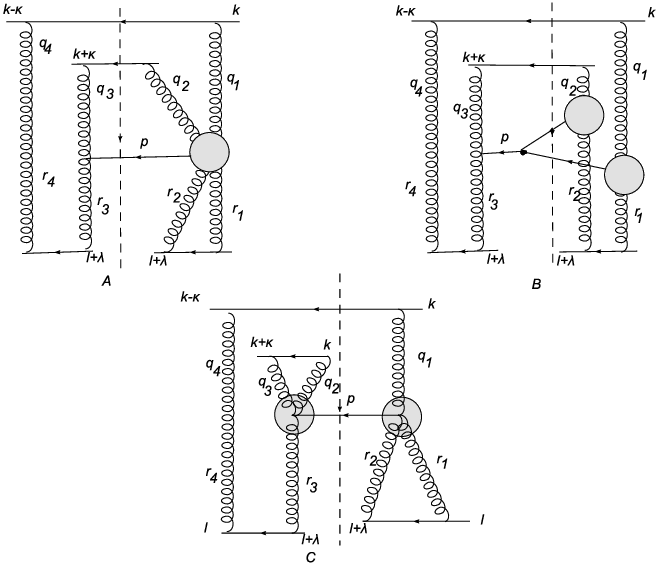
The NLO contributions to the diffractive production of protons off the deuteron with interaction of three pairs of reggeons involve three types of diagrams shown in Fig 1. The bulk of the contribution comes from diagram in Fig. 1,A in which the intermediate gluon is produced by the process R+R$\to$R+R+G where R stands for reggeon and G for gluon. In Fig. 1,B we show another contribution to the cross-section with two gluons in the intermediate state. Finally Fig. 1,C shows one more possible diagram for this process in which the intermediate gluon arises from two processes R+R$\to$R+G. However, in fact this latter contribution is canceled between the direct and conjugated diagrams and need not be considered.

To conclude this introduction we recall the basic formulas connecting the diagrams with the cross-section itself. We work in the center-of-mass system of the colliding proton and one of the nucleons of the deuteron. The inclusive cross-section of the diffractive proton production $d(2k)+p(l)\to p(l^{\prime})+X$ is given by

where the amplitude ${\cal A}$ corresponds to Fig. 1. Let the final proton momentum be $l^{\prime}=l+\lambda$. The missing mass is then $M^{2}=-4k_{+}\lambda_{-}$. In terms of the overall and pomeron rapidities $Y$ and $y$ we have $M^{2}=M_{0}^{2}\exp(Y-y)$ where $M_{0}\sim 1$ Gev. Putting $t=|\lambda_{\perp}|^{2}$ we rewrite the diffractive cross-section as

Separating the deuteron lines we standardly find (see [18])

where

$H$ is the high-energy part of ${\cal A}$ and $\kappa_{+}$ is the $+$-component of the momentum $\kappa$ transferred to one of the nucleons in the deuteron with $\kappa_{-}=\kappa_{\perp}=0$. For comparison, in the same process with a heavy nucleus projectile, the contribution from the collision with two nucleons is given by (1) with

where $\rho({\bf b},z_{1})$ is the nuclear density normalized to unity.

The Glauber approximation corresponds to the contribution which follows when $F(z)$ does not depend on $z$. Then the square of the deuteron wave function converts into the average $<1/2\pi r^{2}>$ and in (5) we find integration over the impact parameter ${\bf b}$ of the square of the profile function $T({\bf b})$. In standard cases the high-energy part contains $\delta(\kappa_{+})$:

Then for the deuteron

and for a large nucleus

The paper is organized as follows. In the next section we discuss the main part of the contribution to the high-energy amplitude $H$ corresponding to the transition R+R$\to$R+R+G for the production of the intermediate gluon realized by vertex $\Gamma_{RR\to RRG}$. Next we discuss the two-gluon intermediate state corresponding to Fig. 1,B. In the last section we make some conclusions. Some long and cumbersome calculations are transferred to the three Appendices.

The diagram which describes the NLO corrections due to RR$\to$RRG vertex $\Gamma_{RR\to RRG}$ is shown in Fig. 1,A in the introduction. It should be supplemented by a similar diagram with interchanged nucleons in the deuterons and conjugated contributions. The interchange of the nucleons does not change the amplitude. due to the symmetry of the vertex respective to permutations of both the two incoming reggeons and the outgoing reggeons. So it is sufficient to study the diagram in Fig. 1,A and double its contribution. Vertex $\Gamma_{RR\to RRG}$ itself does not depend on impact factors and does not feel evolution. So finding its contribution can be simplified by suppressing evolution and taking some simple impact factors for the pomerons. We take simple quarks for the four scattering centers assuming that their interaction is due to colorless exchange.

The total number of transferred momenta is 7: $q_{1}$, $q_{2}$, $q_{3}$, $r_{1}$, $r_{2}$, $r_{3}$, and $q_{4}=r_{4}$. The momentum of the real gluon $p$ is $p=q_{1}+q_{2}-r_{1}-r_{2}$. We choose as independent momenta $q_{1}$, $r_{1}$ and $p$. Then we have

So we have 6 longitudinal integrations. There are 5 conditions arising from mass-shell conditions for real intermediate particles and sums of direct and crossed diagrams for the rest, which give:

multiplied by $4s^{2}$. Integration over $q_{1+}$, $q_{1-}$ and $r_{1+}$ are done withe the help of $\delta$-functions, which puts $q_{1+}=\kappa_{+}$, $q_{1-}=r_{1+}=0$. Of the three integrations over $p_{\pm}$ and $r_{1-}$ the $\delta$ functions

allow to integrate over $p_{\pm}$ and we are finally left with only one longitudinal integration over $r_{1-}$ with $p_{-}=-\lambda_{-}$.

Apart from the four pomerons the diagram of Fig. 1,A involves the Lipatov vertex on the left $f^{b_{3}a_{3}c}L(-p,r_{3})$ where $a_{3}$, $b_{3}$ and $c$ are the color indices of the two reggeons 3 (incoming and out going) and of the real gluon. It does not depend on longitudinal variables and enters only the transversal integral. On the right we meet the RR$\to$RRP vertex of the structure

It does depend on longitudinal variables and is symmetric in $r_{1},r_{2}$ and antisymmetric in $q_{1},q_{2}$.

Doing summation over colors we obtain the imaginary part $H_{1}$ coming from Fig. 1,A as

where $\tau_{\perp}$ is the transverse phase volume, $y$ is defined as before via $M^{2}$. We include in each pomeron factor $N_{c}g^{2}$. Then in the final factor just $g^{4}$ appears. Note that $2s^{2}/p_{-}=8s^{2}k_{+}/M^{2}$.

In (9) we have used that the momentum part of $\Gamma$ is antisymmetric under $q_{1+}\leftrightarrow q_{2+}$, since the color factor is antisymmetric under this exchange. In the vertex $\Gamma$ we have to take longitudinal variables in accordance with our results

and the transverse momenta inside the pomerons are constrained by

The interchange of the two projectiles in the deuteron plus complex conjugate contribution multiply (9) by factor 4.

Note that in contrast to more or less trivial cases of the scattering off a composite the obtained expression does not contain $\delta(\kappa_{+})$, which could lift the integration in (4) and bring the resulting cross-section into the Glauber form. In our case $\kappa_{+}$ appears in the cross-section via longitudinal momentum $q_{1+}=\kappa_{+}$. Therefore in (9) after doing the integration over $r_{1-}$ one has to perform integration over $q_{1+}$ with the weight dictated by (4). As we shall see this integration goes over a finite interval of rapidities of the order $\delta$ due to the condition that all intermediate gluons should lie at finite rapidity distances from the real intermediate gluon. After integration over $q_{1+}$ one finds first terms proportional to $\delta$, which should be dropped, since hopefully they are to be canceled by other terms of the same order, namely terms with pairwise interaction between reggeons, with extra BFKL interactions or with this interaction in the second order. The rest terms are well convergent and do not depend on $\delta$ nor on the exponential in (4), since the exponent is small. These terms lead to $F(z)$ independent of $z$ and thus to the same Glauber expression (7) for the amplitude with

As mentioned, the left Lipatov vertex in the diagram in Fig. 1,A is on-shell and does not depend on $r_{1-}$ nor on $q_{1+}$ So we have to longitudinally integrate only the vertex RR$\to$RRP. Therefore combining the coefficients in (9) and (2) our result final result for the cross-section from the vertex $\Gamma$ has the form

where

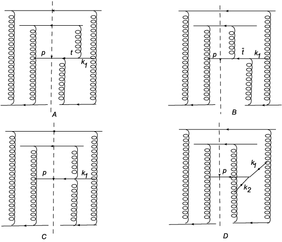
The total vertex $\Gamma$ is a sum of 5 pieces $\Gamma=\sum_{i=1}^{5}\Gamma_{i}$. The diagrams with vertices $\Gamma_{i}$ are shown in Fig. 2.

Actual longitudinal integrations in $\Gamma_{i}$, $i=1,...5$ are long and tedious. They are described in Appendices 1,2 and 3. To avoid proliferation of notations we denote the resulting integrated $\Gamma$ with the same letter $\Gamma$. Collecting our results derived in the appendices, we find for different pieces the following expressions.

where $\hat{T}_{0}$ is given by (59).

where $\hat{T}_{1}$ is given by (63).

where $V_{0}$ is given by (65).

where $V_{1}$ is given by (70). Here $+(Sym)$ means addition of

.

The most complicated part comes from $\Gamma_{5}=\Gamma^{A}+\Gamma^{B}$ We find

where

$\phi_{2}$ is the angle between ${\bf p}$ and ${\bf q}_{2}-{\bf r}_{2}$, $0\leq\phi\leq\pi$ and coefficients $T_{n}$, $U_{0}$ and $V_{0}$ are given by (74).

where

$\phi_{1}$ is the angle between ${\bf p}$ and ${\bf q}_{1}-{\bf r}_{1}$, $0\leq\phi\leq\pi$ and coefficients $\tilde{T}_{n}$, $\tilde{U}_{0}$ and $\tilde{V}_{0}$ are given by (76).

Separate terms in $\Gamma_{3}$, $\Gamma_{4}$ and $\Gamma_{5}$ contain non-integrable divergence at ${\bf q}_{1}\to{\bf r}_{1},{\bf r}_{2}$ and ${\bf q}_{2}\to{\bf r}_{1},{\bf r}_{2}$. However, in Sec. 7.6 it is demonstrated that these singularities cancel in the sum of all $\Gamma_{i}$, $i=3,4,5$.

In (13) the integrated $\Gamma$ is to be multiplied by the Lipatov vertex

The integrated $\Gamma$ contains products $(ae)_{\perp}$ with different $a$. Summation over polarization transforms

So in the end one obtains ${\cal M}$ as a well defined function of transverse momenta ready for practical evaluations.

To begin we find that of the two additional contributions shown in Fig. 1, B and C only the first with two intermediate gluons gives non-zero contribution. Indeed the contribution to the unitarian from the diagram in Fig. 1, C cancels between the amplitude and its conjugated term. In this diagram on the right-hand side (rhs) from the cut we find purely imaginary contribution due to the single incoming reggeon $q_{1}$. On the left-hand side (lhs) we have a similar purely imaginary quantity plus an extra gluon $q_{4}=r_{4}$, which gives $+i$. So the total contribution to the unitarian is imaginary and will be canceled by the conjugated one.

So we are left only with the contribution from the two-gluon intermediate states, Fig. 1, B. This diagram is quite similar to the diagram in Fig. 2,D but with a different cut. This makes its calculation somewhat different.

References

• [1] I.Balitski, Nucl. Phys. B 463 (1996) 99.
• [2] Yu.V.Kovchegov. Phys. Rev. D 60 (1999) 034008.
• [3] Yu.V.Kovchegov, K.Tuchin, Phys. Rev. D 65 (2002) 074026.
• [4] J.Jalilian-Marian, Yu.V.Kovchegov, Phys. Rev. D 70 (2004) 114017.
• [5] A.Krasnitz, R.Venugopalan, Phys. Rev. Lett.84 (2000) 4309; Phys. Rev. Lett.86 (2001) 1717.
• [6] A.Krasnitz, Y.Nara, R.Venugopalan, Phys. Rev. Lett.87 (2001) 192302;
Nucl. Phys. A 727 (2003) 127; Phys. Lett. B 554 (2003) 21.
• [7] T.Lappi, Phys. Rev. C 67 (2003) 054903; Phys. Rev. C 70 (2004) 054905;
Phys. Lett. B 643 (2006) 11.
• [8] Yu.V.Kovchegov, Nucl. Phys. A 692 (2001) 567.
• [9] I.Balitski, Phys. Rev. D 72 (2005) 074027.
• [10] K.Dusling, F.Gelis, T. Lappi, R.Venugopalan, Nucl. Phys. A 836 (2010) 159.
• [11] M.A.Braun, Eur. Phys. Jour. C 73 (2013) :2418.
• [12] M.A.Braun, Eur. Phys. Jour. C 73 (2013) :2511.
• [13] M.A.Braun, Eur.Phys. Jour. C 77 (2017) :277.
• [14] J.Bartels, V.S.Fadin, L.N.Lipatov, G.P.Vacca, Phys. Rev.D 86 (2012) 105045.
• [15] J.Bartels, Nucl. Phys. B 175 (1980) 365.
• [16] J.Kwiecinski, M.Praszalowicz, Phys. Lett. B 94 (1980) 413.
• [17] V.S.Fadin, M.G.Kozlov, A.V.Reznichenko, Phys. Atom. Nucl., 67 (2004) 359
[[hep-ph/0302224]].
• [18] M.A.Braun, M.Yu.Salykin, M.I.Vyazovsky, Eur. Phys. Jour. C 72 (2012) :1864.
• [19] M.A.Braun, S.S.Pozdnyakov, M.Yu.Salykin, M.I.Vyazovsky,
Eur. Phys. Jour. C 75 (2015) :222.