A solution of the minimum-time velocity planning problem
based on lattice theory
Luca Consolini
Mattia Laurini
Marco Locatelli
Andrea Minari
1 Dipartimento di Ingegneria e Architettura, Università degli Studi di Parma,
Parco Area delle Scienze 181/A, 43124 Parma, Italy.
luca.consolini@unipr.it, mattia.laurini@unipr.it, marco.locatelli@unipr.it, andrea.minari2@studenti.unipr.it
Abstract
For a vehicle on an assigned path, we find the minimum-time speed
law that satisfies kinematic and dynamic constraints, related to
maximum speed and maximum tangential and transversal acceleration.
We present a necessary and sufficient condition for the feasibility of the
problem and a simple operator, based on the solution of two ordinary
differential equations, which computes the optimal solution.
Theoretically, we show that the problem feasible set, if not empty, is a
lattice, whose supremum element corresponds to the optimal solution.
An important problem in motion planning is the computation of the
minimum-time motion of a car-like vehicle from a start configuration
to a target one while avoiding collisions (obstacle avoidance) and
satisfying kinematic, dynamic and mechanical constraints (for
instance, on velocities, accelerations and maximal steering
angle). This problem can be approached in two ways:
1.
as a minimum-time trajectory planning where both the
path to be followed by the vehicle and the timing law on this path
(i.e., the vehicle’s velocity) are simultaneously designed; or
2.
as a (geometric) path planning followed by a minimum-time
velocity planning on the planned path
(see for instance [8]).
In this paper, following the second paradigm, we assume that
a path that joins the initial and final configurations, compatible
with the maximum curvature allowed for the car-like vehicle,
is assigned and we aim at finding the time-optimal speed law
that satisfies some kinematic and dynamic constraints.
Previous works address the problem in time domain.
For instance, [16] investigates necessary optimality
conditions that allows deriving a semi-analytical solution.
Reference [7] assumes that the vehicle moves along a
specified clothoid and proposes a semi-analytical solution for the
optimal profile of the longitudinal acceleration.
Some approaches propose special speed profiles that guarantee the
satisfaction of kinematic and dynamic constraints (see for instance
[11, 15, 18, 3]).
Other works (see, for instance, [2, 17, 14, 10, 12])
represent the speed law as a function of the arc-length
position and not as a function of time.
Here, we follow this second approach, that considerably simplifies the optimization problem.
This paper is a development of our previous works
([4, 5]), that consider the following
problem
(1a)
(1b)
(1c)
(1d)
Here, , , , are assigned functions,
with , non-negative.
The objective function (1a) is the total maneuver
time and constraints (1b), (1c), (1d)
limit velocity and the tangential and normal components of acceleration.
Problem (1) belongs to a class of problems that
includes optimal velocity planning for manipulators and has the form
(2)
where is the number of constraints and are assigned functions.
It is clear that Problem (1) is a special case of
Problem (2), obtained for a specific choice of
, , .
Our previous works [4, 5] present an algorithm,
with linear-time computational complexity with respect to the number of
variables, that provides an optimal solution of (1)
after spatial discretization.
Namely, the path is divided into intervals of equal length and
Problem (1) is approximated
with a finite dimensional one in which the derivative of is
substituted with a finite difference approximation.
In this paper, we compute directly the exact continuous-time solution of
Problem (1) without performing a finite-dimensional
reduction.
The main result of the paper is presented in
Theorem 3.1. It gives a sufficient and necessary
condition for the feasibility of Problem (1) and
presents its optimal solution, which is computed as the pointwise minimum
of the solutions of two ODEs.
The method we propose presents some resemblances with the method of
“numerical integration”, introduced for problems of class (2).
For instance, [14] proposes a
method, based on the identification of “characteristic switching
points” in which the maximum velocity is attained. This simplifies the
calculation of the optimal velocity profile. A related algorithm is
presented in [9]. Recent
paper [13] presents various properties of numerical
integration methods.
Anyway, the method we propose is simpler and more efficient since it
leverages the special structure of Problem (1) with
respect to the more general problem (2).
Statement of contribution:
With respect to existing literature, the new contributions of this work are the following ones:
•
It presents a necessary and sufficient condition for the
feasibility of Problem (1) (see part i. of
Theorem 3.1).
•
It proposes a simple operator, based on the solution of two
ordinary differential equations, that computes the optimal solution
(see part ii. of Theorem 3.1).
Note that these results correspond to the generalization to the continuous-time
case of the results presented in [5] for the
spatially-discretized version of Problem (1). In
fact, this paper shares some of its fundamental ideas
with [5]. Namely:
•
The feasible set of
Problem (1) has the algebraic structure of a
lattice, if equipped with the operations of pointwise minimum and
maximum.
•
The optimal solution of Problem (1)
corresponds to the supremal element of this lattice.
•
The optimal solution of Problem (1) is
obtained with a projection operation and its optimality is proven by the
Knaster-Tarski Fixpoint Theorem.
Anyway, solving the problem in a function space requires various nontrivial
technical extensions to the proofs presented in [5].
Notation: Given an interval
and a measurable function , let us recall that
and
where denotes the weak derivative of .
Let , define , ,
as, respectively, the pointwise minimum and maximum operations;
moreover let us define the partial order as follows
We will write “almost everywhere” as “a. e.” and we will use symbol
at the end of a proof to state that a contradiction has been reached.
Paper organization:
Section 2 presents the addressed optimal control
problem. Section 3 presents the main result
(Theorem 3.1) and Section 4 presents
some examples. Finally, Section 5 presents the
proof of the main result.
2 Problem formulation
Let be a function such that
.
The image set represents the path followed
by a vehicle, the initial configuration and the final one.
We want to compute the speed-law that minimizes the overall transfer time while
satisfying some kinematic and dynamic requirements. To this end, let
be a differentiable
monotone increasing function that represents the vehicle position as a function
of time and let
be such that,
In this way, is the vehicle velocity at position s. The position of the vehicle
as a function of time is given by , , the velocity and acceleration are given by
where and
are, respectively, the longitudinal and normal components of acceleration.
Here is the scalar curvature, defined as
We require to travel the distance in minimum-time while
satisfying constraints on the vehicle velocity and on its longitudinal and normal
acceleration.
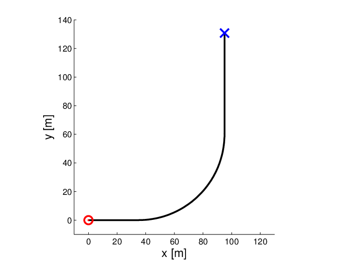
Figure 1: A path to follow for an autonomous car-like vehicle.
The minimum-time problem can be
approached by searching a velocity profile
which is the solution of Problem (1).
It is convenient to make the change of variables (see also [17]), so that
Problem (1) takes on the form
(3a)
(3b)
(3c)
where
(4)
represent the upper bound of ,
(depending on the velocity bound and the curvature ) and
the lower bound of , respectively.
In this paper, we actually address the following problem,
which is slightly more general than (3),
(5a)
(5b)
(5c)
where is order reversing
(i.e., ) and
, , , are
assigned functions with , . Note that the objective
function (3a) is order reversing, so that
Problem (3) has the form (5).
Consider the following:
Definition 2.1.
Let be the subset of such
that if
and are Riemann integrable
(i.e., in view of the boundedness of the function, a. e. continuous),
where is defined as
3 Main Results
Define the forward operator
such that , where is the solution of the following
differential equation
(6)
Note that the solution of (6) exists and is
unique by Theorem 1 in Chapter 2, Section 10
of [1], since function is bounded on , the subset of in which is discontinuous has zero measure and, , ,
Conversely, define the backward operator ,
such that , where is the solution of
(7)
whose existence and uniqueness hold for the same reasons as (6).
Finally, define the meet operator as
(8)
We claim that the meet operator allows checking the
feasibility of Problem (5) and that, in case
Problem (5) is feasible, function
represents its optimal solution.
Namely, the following is the main result of this paper.
Theorem 3.1.
Let , then the following statements hold:
i.
Problem (5) is feasible if and only if function
satisfies
ii.
If Problem (5) is feasible,
then function is its optimal solution.
Proofs of the results.
Part i. follows from Proposition 5.11,
part ii. follows from Proposition 5.12 (see Section 5).
4 Examples
As a first example consider the path shown in
Figure 2, whose
curvature is defined as
(9)
where is the 6-th degree Hermite polynomial used to guarantee
the following interpolation conditions:
Figure 2: On the left, the curvature function
in (9) of the curve discussed in the first example. On
the right, the black line represents the path, the red circle and the black cross represent the
starting point and, respectively, the end point.
In this example, the total length is
and the minimum-time velocity planning problem is addressed with
, .
The velocity bounds and are set as follows: ,
, while, for each ,
and .
The longitudinal acceleration limits are and
, and the maximal normal acceleration is .
The following results are obtained by numerically solving
equations (6), (7)
with a standart Runge-Kutta 45 integration
scheme. Figure 3 shows the upper-bound
function
obtained
by (4) and the corresponding functions and
computed as the solution of equations (6) and (7), respectively.
Figure 4 shows the optimal solution obtained with (8).
In this example, the vehicle starts with zero velocity and accelerates
to the upper bound. Then, it follows the velocity bound
in order to respect the
maximum velocity constraint due to the lateral acceleration on the curve.
After that, at the end of the constant bound, the vehicle accelerates and reaches a second local
maximum velocity after which it decelerates quickly in order to reach the final
velocity .
Figure 3: Example 1: The red line represents function
defined in (4), the blue line represents
while the green line represents .Figure 4: Example 1: The red line
represents defined in (4), the black line represents
the optimal solution .
As a second example, consider the same path and constraints as in the
first example, with different initial
and final conditions: ,
.
Figure 5 shows function obtained by (8).
In this case, Problem (5) is unfeasible by
Theorem 3.1, being .
In fact, the allowed maximum longitudinal acceleration is not sufficient to
reach the final condition on velocity.
Figure 5: Example 2. The green line represents
the velocity function while the black one depicts function .
The final velocity condition is not satisfied: .
As a third example, consider a curve obtained by a quintic
polynomial curve which interpolates coordinates ,
(see Figure 6).
The velocity planning is addressed with
, and with
and for each .
The longitudinal acceleration limits are
, ,
and the maximal normal acceleration .
The resulting optimal velocity profile is plotted in
Figure 7.
Figure 6: A path obtained by quintic-splines interpolation. The black line represents
the path while the circle and the cross represent the start and the end point, respectively.Figure 7: The red line represents function defined
in (4), the black line is the optimal velocity profile .
5 Proofs
Given the interval ,
let .
Note that is a complete lattice.
Hence, for each subset , there exists a unique least upper bound
, such that,
The least upper bound of is denoted by .
Dually, it is possible to define the greatest lower bound of ,
denoted by (see Definitions 2.1, 2.4 and Notation 2.3 on
pages 33-34 of [6]).
Given function defined as follows
let us define , function as
(10)
Define, also, operators , such that,
for , and are given as follows
and .
Observe that ,
(11)
As we will show in Proposition 5.9, the operators we just
introduced are extensions of those defined, respectively,
in (6), (7)
and (8).
We will refer to the following definitions.
Definition 5.1.
An operator is meet preserving if, ,
Definition 5.2.
An operator is order preserving if, ,
Even though we will only use the fact that operators and
are order preserving, for completeness we state the following Proposition.
Proposition 5.3.
Operators , and are meet preserving and order preserving.
Proof.
Let , .
We want to show that .
By definition of we have that and
,
The proof that is analogous.
Finally, .
Since maps are meet preserving, they are also order preserving
(see Proposition 2.19 on page 44 of [6]).
∎
Proposition 5.4.
Function defined as in (10) is a
hemi-metric, that is, it satisfies the following properties:
i.
,
ii.
,
iii.
(i.e., the triangular inequality holds). Moreover, equality holds if or .
Proof.
i.
It holds, since is non-negative
and is non-positive over .
ii.
It holds trivially by definition of .
iii.
For :
The same reasoning applies also to the case when ,
or .
Next, let us show that equality holds for any :
The proof that the equality holds also for any is analogous.
∎
Proposition 5.5.
Function satisfies the following properties, ,
i.
,
ii.
, where
stands for .
Proof.
i.
It is a consequence of the definition of .
ii.
Let us now show that :
the fact that follows by the definition of whilst,
to prove the opposite inequality, note that, by Proposition 5.4 and
(11),
In the same way it can be proved that , from which it follows that
.
∎
Proposition 5.6.
Proof.
Set .
Note that is a sublattice of ,
moreover, by i. of Proposition 5.5, if ,
then .
Since is order preserving by Proposition 5.3,
by the Knaster-Tarski Fixpoint Theorem
(Theorem 2.35 on page 50 in [6])
is such that is the greatest fixed point of such that .
Let , by part ii. of Proposition 5.5, we know
that is also a fixed point of , thus, by definition of , .
To prove that , that is, to prove that is also the greatest fixed point,
it remains to show that .
To this end, assume, by contradiction, that .
Since , and the fact that is order preserving,
it follows that , which contradicts the definition of .
∎
Remark 5.7.
Given , if , this does not imply that and ,
as and may not be comparable with respect to partial order .
Proposition 5.8.
The following two statements are equivalent:
i.
Set is not empty.
ii.
.
Proof.
It follows from the fact that is such that
by part ii. of Proposition 5.5.
By contradiction, assume that .
Choose any such that and .
By Proposition 5.6,
, hence ,
but , so .
Thus, being any fixed point of such that ,
set is empty .
∎
Proposition 5.9.
If ,
then satisfy a. e.
(12)
and
(13)
Proof.
Let .
Note that, since , contains almost all elements of .
Let , then
(14)
Since by Proposition 5.4,
the first parenthesis of (14) reduces to
Being continuous at , it is possible to choose
sufficiently small such that is constant on interval
.
Set and
.
Then, the second parenthesis of (14) can be rewritten as
since in the former case the minimum of over
is attained at , whilst in the latter is attained at .
Hence, we have that
Note that, by definition of , must hold.
In conclusion, we proved that
and satisfies (12).
Applying the same reasoning it can be proved that
and satisfies (13).
∎
Proposition 5.10.
Assume that and let ,
then is feasible for Problem (5)
(i.e., it satisfies constraints (5b) and (5c)),
if and only if and .
Proof.
Assume that is feasible for
Problem (5), then satisfies a. e.
. Thus, is the solution
of (6) for , which implies that
.
Analogously , so that .
Moreover, since satisfies the bounds of Problem (5),
it follows that .
Condition (5b) holds by hypothesis.
Since , then it must be . In fact, if
by contradiction , , which contradicts
the assumption .
Then , implies that, a. e., which
by definition of in (6), implies that, a. e., .
Analogously, it must be which implies that, a. e. and condition (5c) holds.
∎
Proposition 5.11.
Assume that .
Then, Problem (5) is feasible if and only if .
Proof.
Let be a feasible solution of
Problem (5). Then, by
Proposition 5.10, .
Hence, being order preserving, .
satisfies (by part ii. of
Proposition 5.5) and (by
hypothesis). Hence, by Proposition 5.10, is a feasible
solution of Problem (5).
∎
Proposition 5.12.
If and Problem (5)
is feasible, then is its optimal solution.
Proof.
By contradiction, assume that there exists a feasible such that
. Since is feasible,
Proposition 5.10 implies that .
Moreover, since is order reversing, .
This is not possible since , by Proposition 5.6 .
∎
References
[1]
F. Arscott and A. Filippov.
Differential Equations with Discontinuous Righthand Sides:
Control Systems.
Mathematics and its Applications. Springer Netherlands, 2013.
[2]
J. Bobrow, S. Dubowsky, and J. Gibson.
Time-optimal control of robotic manipulators along specified paths.
The International Journal of Robotics Research, 4(3):3–17,
1985.
[3]
C. Chen, Y. He, C. Bu, J. Han, and X. Zhang.
Quartic Bézier curve based trajectory generation for autonomous
vehicles with curvature and velocity constraints.
In Robotics and Automation (ICRA), 2014 IEEE International
Conference on, pages 6108–6113, May 2014.
[4]
L. Consolini, M. Locatelli, A. Minari, and A. Piazzi.
A linear-time algorithm for minimum-time velocity planning of
autonomous vehicles.
In Proceedings of the 24th Mediterranean Conference on Control
and Automation (MED), IEEE, 2016.
[5]
L. Consolini, M. Locatelli, A. Minari, and A. Piazzi.
An optimal complexity algorithm for minimum-time velocity planning.
Systems & Control Letters, 103:50–57, 2017.
[6]
B. Davey and H. Priestley.
Introduction to Lattices and Order.
Cambridge University Press, 2002.
[7]
M. Frego, E. Bertolazzi, F. Biral, D. Fontanelli, and L. Palopoli.
Semi-analytical minimum time solutions for a vehicle following
clothoid-based trajectory subject to velocity constraints.
In 2016 European Control Conference (ECC), pages 2221–2227,
June 2016.
[8]
K. Kant and S. W. Zucker.
Toward efficient trajectory planning: The path-velocity
decomposition.
The International Journal of Robotics Research, 5(3):72–89,
1986.
[9]
T. Kunz and M. Stilman.
Time-optimal trajectory generation for path following with bounded
acceleration and velocity.
Robotics: Science and Systems VIII, 2012.
[10]
X. Li, Z. Sun, A. Kurt, and Q. Zhu.
A sampling-based local trajectory planner for autonomous driving
along a reference path.
In Intelligent Vehicles Symposium Proceedings, 2014 IEEE, pages
376–381, June 2014.
[11]
V. Muñoz, A. Ollero, M. Prado, and A. Simón.
Mobile robot trajectory planning with dynamic and kinematic
constraints.
In Proc. of the 1994 IEEE Int. Conf. on Robotics and
Automation, volume 4, pages 2802–2807, San Diego, CA, May 1994.
[12]
Á. Nagy and I. Vajk.
Lp-based velocity profile generation for robotic manipulators.
International Journal of Control, pages 1–11, 2017.
[13]
P. Shen, X. Zhang, and Y. Fang.
Essential properties of numerical integration for time-optimal
path-constrained trajectory planning.
IEEE Robotics and Automation Letters, 2(2):888–895, April
2017.
[14]
J. J. E. Slotine and H. S. Yang.
Improving the efficiency of time-optimal path-following algorithms.
IEEE Transactions on Robotics and Automation, 5(1):118–124,
Feb 1989.
[15]
R. Solea and U. Nunes.
Trajectory planning with velocity planner for fully-automated
passenger vehicles.
In IEEE Intelligent Transportation Systems Conference, ITSC
’06, pages 474 –480, September 2006.
[16]
E. Velenis and P. Tsiotras.
Minimum-time travel for a vehicle with acceleration limits:
Theoretical analysis and receding-horizon implementation.
Journal of Optimization Theory and Applications,
138(2):275–296, 2008.
[17]
D. Verscheure, B. Demeulenaere, J. Swevers, J. D. Schutter, and M. Diehl.
Time-optimal path tracking for robots: A convex optimization
approach.
IEEE Transactions on Automatic Control, 54(10), Oct 2009.
[18]
J. Villagra, V. Milanés, J. Pérez, and J. Godoy.
Smooth path and speed planning for an automated public transport
vehicle.
Robotics and Autonomous Systems, 60:252–265, 2012.