On the Question of Ergodicity in Quantum Spin Glass Phase and its role in Quantum Annealing
Abstract
We first review, following our earlier studies, the critical behavior of the quantum Sherrington-Kirkpatrick (SK) model at finite as well as at zero temperatures. Through the analysis of the Binder cumulant we determined the entire phase diagram of the model and from the scaling analysis of the numerical data we obtained the correlation length exponent. For both the critical Binder cumulant and the correlation length exponent, we observed a crossover from classical- to quantum-fluctuation-dominated values at a finite temperature. We studied the behavior of the order parameter distribution of the model in the glass phase (at finite and zero temperatures). Along with a classical-fluctuation-dominated nonergodic region (where the replica symmetry is broken), we also found a quantum-fluctuation-dominated low-temperature ergodic region in the spin glass phase. In this quantum-fluctuation-dominated region, the order parameter distribution has a narrow peak around its most probable value, eventually becoming a delta function in the infinite-system-size limit (indicating replica symmetry restoration or ergodicity in the system). We also found that the annealing time (to reach a very low energy level of the classical SK model) becomes practically system-size-independent when the annealing paths pass through this ergodic region. In contrast, when such paths pass through the nonergodic region, the convergence time grows rapidly with the system size. We present a new study of the autocorrelation of the spins in both ergodic and nonergodic regions. We found a significant increase in the relaxation time (and also a change in the relaxation behavior) in the classical-fluctuation-dominated (nonergodic) region compared with that in the quantum-fluctuation-dominated (ergodic) region of the spin glass phase.
I Introduction
Spin glasses [1] have many intriguing features in their thermodynamic phases and transition behaviors. The effects of quantum fluctuations on such spin glass phases are being investigated extensively these days in the context of the physics of quantum glasses and information processing. For this, we have chosen quantum Ising spin glass models [2, 3]. We focus our study on the Sherrington-Kirkpatrick (SK) spin glass model [1] in the presence of a transverse field [3]. Many studies have already been carried out (see e.g., Refs. [4, 5, 6, 7, 8, 9, 10]) to extract some isolated features of the quantum phase transitions of the SK model. We have performed detailed numerical studies of the critical behavior of this model at finite temperatures as well as at zero temperature. We have numerically extracted the entire phase diagram of the model. The finite-temperature analysis was carried out by Monte Carlo simulation and the zero temperature critical behavior was obtained using the exact diagonalization method. From both of these numerical techniques we calculated the critical Binder cumulant [11], which gives the phase boundary and also the nature of the phase transitions. We found the correlation length exponent from the scaling behavior of the Binder cumulant with the system size. Such studies revealed the value of the critical Binder cumulant and the correlation length exponent, also giving the point of crossover from their ‘classical’ behavior (associated with the classical SK model) to ‘quantum’ behavior (corresponding to that at zero temperature). Interestingly, this crossover happens at a finite temperature.
Due to the random and competing spin-spin interaction, the free-energy landscape of a spin glass system is highly rugged. Local minima are often separated by macroscopically high free-energy barriers, which are often on the order of the system size (escape requiring a macroscopic fraction of spins to be reversed). This feature of the free-energy landscape induces nonergodicity in the system. The system very often becomes trapped at one of the local minima. As a consequence, the phenomenon of replica symmetry breaking is observed in the spin glass phase and the order parameter follows a broad distribution. Along with a peak at nonzero value of the order parameter, the distribution also contains a tail that extends up to the zero value of the order parameter. This extended tail does not vanish even in the thermodynamic limit. Such an order parameter distribution in the spin glass phase was suggested by Parisi [12].
When an SK glass is placed under a transverse field the situation becomes considerably different. In the presence of quantum fluctuation the system can tunnel through the high (but narrow) free-energy barriers [13, 14, 15, 16, 18, 17] which essentially allows the system to avoid becoming trapped at local free-energy minima. This phenomenon of quantum tunneling often helps the system to regain ergodicity and one can expect the absence of replica symmetry breaking in the spin glass phase. As a result, the order parameter distribution has a narrow peak around some nonzero value of the order parameter, which essentially should be a delta function in the thermodynamic limit [13].
We numerically study the behavior of the order parameter in the spin glass phase of the quantum SK model at both finite and zero temperatures. From such investigations we identify a low-temperature (high-transverse-field) ergodic region in the spin glass phase, where the tail of the order parameter distribution vanishes in the thermodynamic limit (indicating the convergence of the distribution to one with a sharp peak around the most probable value). This suggests the ergodic (or replica-symmetry-restored) nature of the system in this region of the spin glass phase. In the rest of the spin glass phase, we find that the tail of the order parameter distribution does not disappear even for an infinite system size. Thus the order parameter distribution remains the Parisi type [12] (replica-symmetry-broken, indicating nonergodicity) in this region of the spin glass phase. We also carry out dynamical study of the system to find the variation of the annealing time in both the ergodic and nonergodic regions. We find that the annealing time to reach a low-energy state from the paramagnetic phase becomes independent of system the size in the case of annealing down through the ergodic region. On the other hand, the annealing time grows rapidly with the system size when the same annealing is performed through the nonergodic region. These discussions in the following sects. III and V are essentially based on our earlier publications [19, 20].
We add a new study on spin autocorrelation in the glass phase (see sect. VI). We observe that the relaxation behavior of autocorrelation is markedly different in the ergodic and nonergodic regions. The effective relaxation time of the system is much higher in the classical fluctuation dominated (nonergodic) region, whereas the system relaxes very quickly in the quantum-fluctuation-dominated (ergodic) region of the spin glass phase.


II Model
The Hamiltonian of the quantum SK model with Ising spins is given by
| (1) |
Here , are spin-spin interactions and they are distributed with the Gaussian distribution . The mean and standard deviation of the distribution are and , respectively. In this work we set . and are the and components of Pauli spin matrices respectively. The transverse field is denoted by . Using the Suzuki-Trotter formalism we obtain the effective classical Hamiltonian from Eq. (1) to perform Monte Carlo simulations at finite temperatures. The effective classical Hamiltonian is given by
| (2) |
Here is the classical Ising spin and is the inverse of the temperature . We can see the appearance of an additional direction in Eq. (2), which is often called the Trotter direction. The number of Trotter slices is denoted by . In the limit , tends to infinity.
III Study of critical behavior at finite and zero temperature
We numerically estimate the phase diagram of the quantum SK model [19]. To find the critical transverse field or temperature we use the Binder cumulant technique. From the collapse of the of Binder cumulant curves for different system sizes we estimate the correlation length exponent. We notice a crossover in the values of the critical Binder cumulant and correlation length exponent at a finite temperature.
III.1 Monte Carlo results
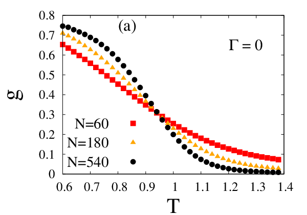
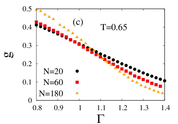
To extract the critical behavior of the quantum SK model at a finite temperature we perform Monte Carlo simulations on the Hamiltonian in Eq. (2). For the study of classical SK model we simulate the Hamiltonian . In each Monte Carlo step we calculate the replica overlap , where and are the spins of two different replicas and , respectively corresponding to identical sets of disorder. We first allow the system to equilibrate with Monte Carlo steps then we perform thermal averaging over next Monte Carlo steps. We study the variation of the average Binder cumulant with (for fixed ) and (for fixed ) for different system sizes. In our calculation the average Binder cumulant is defined as [21, 22]
| (3) |
Here the overhead bar indicates averaging over the configurations and denotes the thermal averaging. We note that the average Binder cumulant can be also defined as . With this definition of one obtains a large fluctuation and poor statistics [21]. Thus, throughout of our calculation we work with the definition of in Eq. (3).
The scaling relation of near the critical region is given by [21]. Here is the linear size of the system and is the Trotter size. The dynamical exponent and correlation length are denoted by and , respectively. The correlation length scales as or with correlation exponents and . The critical temperature and transverse field are denoted by and , respectively. Therefore the scaling relation of can be rewritten as
| (4) |
Here and . We correlate the linear dimension with the total number of spins through the relation , where is the effective dimension of the system. We estimate the values of the critical transverse field and critical Binder cumulant from the intersection of the versus curves for different system sizes (keeping fixed). Using the scaling relation in Eq. (4) we collapse the curves and estimate the values of and .
We simulate the Hamiltonian in Eq. (2) with system sizes . We start with for the system size , and to keep fixed we take for the system sizes , respectively. Here we consider and [23], which are associated with the classical SK model. As there is no additional Trotter dimension in the Hamiltonian , we are able to perform Monte Carlo simulations of the classical SK model with larger system sizes . We take Monte Carlo steps for the equilibration of the system and the thermal average is taken the over the next Monte Carlo steps. The disorder averaging is carried out over samples. We observe that in the range starting from the classical SK model at to almost (), the value of stays almost constant at [see Figs. 1(a), 1(c), and 1(e)]. We also find a satisfactory data collapse of curves with [see Figs. 1(b), 1(d), and 1(f)]. We find that the value of becomes vanishingly small in the range () to (), but in this case we are unable to collapse the curves for any of the chosen values of . In this range we repeat our simulation with and , which are values related to the quantum SK model [24, 25]. In order to keep constant with these new values of and , we take Trotter sizes for the system sizes , respectively. We again notice that the value of becomes almost zero [see Figs. 2(a) and 2(c)] and this time we obtains a satisfactory data collapse of curves [see Figs. 2(b) and 2(d)] with . Note that, with the quantum values of and we are unable to collapse the curves consistently in the range (, ) to (, ). Therefore, we find a change in the values of and at low temperatures. To confirm this observation we investigate the variation of with for a fixed value of . This variation for is shown in Fig. 3(a) and the corresponding data collapse with is shown in Fig. 3(b). This implies that at low temperatures (high ) the critical exponents are . The crossover in the values of and () with the (or ) values within this range (, ) may be abrupt. From our numerical studies here it is not possible to state firmly whether this crossover is gradual or abrupt.


III.2 Zero-temperature diagonalization results
We explore the zero-temperature critical behavior of the SK model through Binder cumulant analysis using the exact diagonalization technique. The diagonalization of the quantum spin glass is performed using the Lanczos algorithm. In the zero-temperature analysis we are able to work with the system sizes only up to . We construct the Hamiltonian Eq. (1) in the spin basis, which is made up of the eigenstates of . The th eigenstate of can be expressed as . Here are the eigenstates of with expansion coefficients . For the zero-temperature analysis we define the order parameter as . Since our interest is focused on zero-temperature analysis, we are confined to ground state () averaging in the evaluation of the order parameter and other physical quantities. In this case the configuration average is again indicated by the overhead bar. The various moments of the order parameter can be calculated using the relation [1, 26],
| (5) |
Physically the are the -spin correlation functions for a given disorder configuration. In the case of zero-temperature, using Eq. (5) we can define the Binder cumulant as .
The variations of as a function of (at ) for different system sizes are shown in Fig. 4(a). The finite-size effects in the estimations of and are quite evident due to the noncoincidence of the intersection points of the curves associated with the different system sizes. To account for this finite-size effect we evaluate the values of and from the intersection of the vs curves for the two system sizes and . Accounting for all possible pairs, we extrapolate as a function of to find in the thermodynamic limit. Due to the absence of any known finite-size scaling behavior of , we extrapolate as a function of to obtain the critical Binder cumulant value for an infinite system size. The best fitting of against is obtained for , and the extrapolated value of is [see Fig. 5(a)]. Considering the estimated critical transverse field and , we also obtain a satisfactory data collapse of the curves associated with the different system sizes [see Fig. 4(b)]. From the extrapolation of we find that in the limit the value of becomes very near to zero [see Fig. 5(b)]. This observation is consistent with the Monte Carlo results at low temperatures. Thus, we can conclude that starting from around to the values of as well as remain constant at and .

III.3 Phase diagram
From the numerical results of the Monte Carlo simulations and the exact diagonalization related to the calculation of the Binder cumulant, we estimate the entire phase diagram (see Fig. 6) of the quantum SK spin glass. From the exploration of this phase diagram, we find that the value of remains fairly constant at in the range () to (). In this range the phase transitions are dominated by classical fluctuation (high and low ). On the other hand, beyond the point () to the quantum transition point (, ) the critical Binder cumulant assumes a very low value () and the phase transitions are predominantly governed by quantum fluctuation (at low and high ). The two values of indicate two distinct universality classes in the critical behavior of the SK spin glass. To confirm the existence of two different universality classes we calculate the correlation length exponent on the two parts of the phase boundary associated with the two different values of . In the case of classical fluctuation dominated phase transitions, if we consider [23] and , then using the relation we find that . This value of is consistent with the earlier estimation of the correlation length exponent of the classical SK model [23]. Similarly, for quantum fluctuation dominated transitions with [24, 25] and we obtain , which again shows good agreement with the earlier estimates [24, 25]. Such changes in the values of and clearly indicate a finite temperature crossover between classical and quantum fluctuation dominated critical behaviors in an SK spin glass.
IV Study of order distribution at finite and zero temperature
To probe the issue of ergodicity in the spin glass phase we investigate the nature of the order parameter distribution at both finite and zero temperatures [20]. Such study clearly indicates two distinct behaviors of the order parameter distribution in two different regions of the spin glass phase, from which we are able to identify the ergodic and nonergodic regions in the spin glass phase.


IV.1 Results of Monte Carlo simulations
To find the order parameter distribution in the spin glass phase at finite temperatures, we perform Monte Carlo simulations on the effective classical Hamiltonian . We define the order parameter of the system as . Therefore, the order parameter distribution can be evaluated as . For a given set of and we compute both area-normalized and peak-normalized order parameter distributions. In the case of peak normalization the distribution is normalized by its maximum value.
For the finite temperature study, we perform Monte Carlo simulations with system sizes and Trotter slices. We notice that the equilibrium time of the system is not uniform throughout the entire plane. Within the region and the system (for ) typically takes time steps for equilibration, whereas the equilibrium time becomes for the rest of the spin glass phase region. The thermal average is taken over time steps and we take samples for disorder averaging. As the system has symmetry we evaluate the distribution of instead of . We notice a system size dependence of the value of . To find the value of in the thermodynamic limit we extrapolate it as a function of . In addition to the finite-size scaling of , we also estimate the value of for an infinite system size. Here is the width of the distribution function and is defined as . The distribution function becomes half of its maximum at and . In the spin glass phase we find two distinct natures of the extrapolated values of both and . At low-temperature (high-transverse-field) the values of both and tend to zero as the system size goes to infinity [see Fig. 7(a)]. This observation indicates that in the thermodynamic limit approaches the Gaussian form, which essentially suggests the ergodic behavior of the system. In contrast to this scenario, we also find a region (high and low ) in the spin glass phase where neither nor vanishes even in the thermodynamic limit [see Fig. 7(b)]. There seems to be no possibility of approaching a distribution with the Gaussian form in the large-system-size limit. Such behavior of indicates that the system is nonergodic in this region of the spin glass phase. For more accurate measures of the ergodic and nonergodic regions in the spin glass phase, we also extract the behavior of the peak-normalized order parameter distribution. Again we find that and of the peak-normalized distribution go to zero in the thermodynamic limit in this region of the spin glass phase, which has already been identified as the ergodic region from the study of the area-normalized distribution. This feature of the peak normalized distribution is shown in Figs. 8(a) and 8(b). Similarly to the area-normalized distribution, at high temperature and low transverse field the values of and for the peak-normalized distribution remain finite even in the large-system-size limit [see Figs. 9(a) and 9(b)].


IV.2 Results of zero temperature exact diagonalizations
We use the exact diagonalization technique to study the nature of the order parameter distribution at zero temperature. The exact diagonalization of the quantum spin glass Hamiltonian [Eq. (1)] is carried out by the Lanczos algorithm. Using this algorithm we evaluate the ground state of the system up to the system size . At zero temperature the order parameter of the system is defined as . Here denotes the site-dependent local order parameter, and the corresponding distribution of the local order parameter is given by We numerically calculate for the system sizes , which are very small. We study the behaviors of for several values of (at ) in the spin glass phase. Similarly to the finite-temperature analysis, we investigate both the area- and peak-normalized [see Figs. 10(a) and 10(b)]. When the system is in the spin glass state, shows a peak at a finite value of along with a nonzero weight at . Although one can find an upward rise of as , the value of decreases with increasing system size. In order to find the nature of both the area- and peak-normalized in the thermodynamic limit, we extrapolate as a function of for each values of . The extrapolations of at the values and [for Fig. 10(a)] and and [for Fig. 10(b)] are shown in the top insets. We also study the finite-size scaling of , where the becomes half of its maximum value at and . We extrapolate as a function of to find its value in the large-system-size limit [see the bottom insets of Figs. 10(a) and 10(b)]. Although due to the severe limitation of the maximum system size, the extrapolated curve does not take a delta-function-like shape, the distribution clearly becomes narrower with the increase in system sizes. The limitation in the system size also be the reason for observing a nonzero value of even in the thermodynamic limit. However, we infer that at zero temperature for any finite value of , the curve will eventually become a delta function at a finite value of in the thermodynamic limit.


V Annealing through ergodic and nonergodic regions
Our investigations in the earlier sections clearly indicate the existence of a high-temperature (low-transverse-field) nonergodic region as well as a low-temperature (high-transverse-field) ergodic region in the spin glass phase. The line separating these two regions starts from , and intersects the spin glass phase boundary at the quantum-classical crossover point [19, 27]. To find the dynamical features of these two regions, we study the annealing dynamics of the system through several paths using with time-dependent and . We vary the temperature and transverse field following the schedules and , respectively. We choose and in such a way that the corresponding points on the phase diagram belong to the paramagnetic phase. In addition, they are equidistant from the critical line in the different parts of the phase diagram. We study the variation of the required annealing time of the system to achieve a very low free-energy associated with the very small values of . At the end of the annealing schedule, we are forced to keep such small but nonzero values of the driving parameters to avoid the singularities in and the annealing dynamics. We investigate the annealing of the system for a path that either passes through the quantum fluctuation dominated or classical fluctuation dominated [see Fig. 11(a)] regions. Our numerical results show that when the annealing paths pass completely through the ergodic region, the annealing time becomes exclusively system-size-independent [see Fig. 11(b)]. In contrast, for the paths that entirely lie in the nonergodic region, the annealing time increases monotonically with increasing , a quantity measuring the arc-distance of the annealing line from the pure quantum () transition point along the phase boundary [see Fig. 11(b)]. We find that the numerical error in estimating the value of , also increases monotonically with increasing . In fact for , the error bars in for different values start overlapping [see Fig. 11(b)]. These results further confirm our earlier observation regarding the annealing time behavior reported in Ref. [20].


VI Study of spin autocorrelation dynamics
We study the autocorrelation of the spins in both the ergodic and nonergodic regions of the spin glass phase. For fixed values of and , after the equilibrium we consider a spin configuration (for a given disorder) at any particular Monte Carlo step . Then we compute the instantaneous overlap of this spin configuration (at ) with the spin states pertaining to the consecutive Monte Carlo steps. We carry out this calculation for an interval of time , then with the spin profile at , we repeat the same calculation for next Monte Carlo steps. For a given system size the autocorrelation function is defined as
| (6) |
For each set of disorder we average over several intervals, which is denoted by . The disorder averaging is denoted by the overhead bar. Since we perform this calculation in the spin glass phase, the autocorrelation should decay to a finite value. We investigate the variation of in both the ergodic and nonergodic regions and we notice a considerable difference in the relaxation behavior in these two regions. In the ergodic region the decay rate of the autocorrelation towards its equilibrium value is much faster than the decay rate in the nonergodic region.
We perform Monte Carlo simulations with system sizes and Trotter slices. The interval average is taken over intervals and in each interval we consider Monte Carlo steps. The disorder average is taken over samples. The variation of with for and is shown in Fig. 12(a). We can see that the autocorrelation very quickly saturates (almost) to its equilibrium value. One can also see the system size dependence of . Therefore, we extract the autocorrelation for an infinite system size through the extrapolation of as a function of . Such extrapolations at are shown in the inset of Fig. 12(a). A similar plot of for and (belonging to the nonergodic region) is shown in Fig. 12(b). One can clearly observe that in this case the decay of the autocorrelation is much slower than in the previous case. To estimate the relaxation time scale in the ergodic and nonergodic regions for an infinite system size, we try to fit the extrapolated curves with the function
| (7) |
Here is the tentative saturation value of for the long-time limit and is the stretched exponent. We refer to as the effective relaxation time of the system. The extrapolated curves belong to the ergodic region and their corresponding best-fit lines are shown in Fig. 12(c). Since the fall of such curves is extremely rapid, the fitting value of is very high (). The relaxation time in the ergodic region is typically on the order of . The variations of with in the nonergodic region with their associated best-fit lines are shown in Fig. 12(d). We find reasonably good fitting by considering but here we find that increases as we move deep into the nonergodic region from the line of separation between the ergodic and nonergodic regions. In Table 1 we present the numerical results obtained from the fittings of curves. From the numerical data we can clearly observe that similarly to critical exponent , there is also a change in the value of the exponent when we move from the ergodic to nonergodic region. Note, that the variations of only four typical points in each of the SG(E) and SG(NE) regions are shown in Figs. 12(c) and 12(d) [and analyzed with Eq.(7)]. Additional investigation for several other points in the regions also suggest similar conclusions.
| , | ||||
|---|---|---|---|---|
| Ergodic | , | |||
| (SG) | , | |||
| , | ||||
| , | ||||
| Non- | , | |||
| ergodic | , | |||
| (SG) | , |
VII Summary and discussion
In sects. III-V we reviewed some of our earlier observations regarding the main question of our study here, and in sect. VI we reported our study of the autocorrelation behavior in the same model, confirming the earlier findings.
We first discussed in sect. III the determination of the phase diagram of the quantum SK model (see Fig. 6) employing the Monte Carlo simulation (at finite temperatures) and exact diagonalization technique (at zero temperature). To extract the critical behavior at finite , we considered system sizes and chose the value of in accordance with the system size, keeping constant. At , we have a severe limitation of the system size (maximum ). Here and respectively denote the effective dimension and dynamical exponent of the system. We found that from the quantum transition point (, ) to almost the point (, ), the critical Binder cumulant () remains vanishingly small. Note that the critical Binder cumulant can effectively vanish even for (non-Gaussian) fluctuation-induced phase transitions [28]. In this range of the phase boundary, we find the correlation length exponent from the data collapse of Binder cumulant plots. In the rest of the phase boundary, the critical Binder cumulant is and we observed a satisfactory data collapse with . These two different values of and for the two different parts of the phase boundary indicate the classical to quantum crossover (at and ) in the quantum SK model.
Unlike in the pure system, where the free-energy landscape is smoothly inclined towards the global minima, in the SK spin glass the landscape is extremely rugged. In particular, the local minima are often separated by macroscopically high energy barriers, inducing nonergodicity and a consequent replica-symmetry-broken distribution of the order parameter. Therefore, at any finite temperature the thermal fluctuation is unable to help the localized system to escape from the free-energy barriers to reach the ground state (by flipping finite fraction of spins). With the aid of the transverse field the system can tunnel through such free-energy barriers [13, 14, 15]. As a consequence, at low temperatures, the phase transition is governed by the quantum fluctuation and the system essentially exhibits quantum critical behavior.
We next studied (see sect. IV) the nature of the order parameter distribution in the spin glass phase at finite temperatures through Monte Carlo simulations. For this numerical study we took and [fixed; for small values, numerical results for were found to remain fairly unchanged even when we varied with keeping constant]. We found [see Figs. 7(b), 9(a), and 9(b)] that in the high-temperature (low-transverse-field) classical fluctuation dominated spin glass region, along with the peak at the most probable value of the order parameter, the distribution contains a long tail (extending up to the zero value of the order parameter). This tail does not vanish even in the limit, which shows that the order parameter distribution remains Parisi type, corresponding to the nonergodic region SG(NE) [see Fig. 11(a)] of the spin glass phase. On the other hand, we found [see Figs. 7(a), 8(a), and 8(b)] a low-temperature high-transverse-field region, where the order parameter distribution effectively converges to a Gaussian form (with a peak around the most probable value) in the infinite-system-size limit. This indicates the existence of a single (replica-symmetric) order parameter in this ergodic region SG(E) of the spin glass phase. At zero temperature, we considered system sizes and . Even with this limitation of the system size, the extrapolated order parameter distribution function showed [see Fig. 10(a)] a clear tendency to become one with a sharp peak (around the most probable value) in the large-system-size limit. We therefore conclude that the ergodic and nonergodic regions of the spin glass phase are separated by a line possibly originating from point () and extending up to the quantum-classical crossover point (, ) [19, 27] on the phase boundary [see Fig. 11(a)].
To find the role of such quantum-fluctuation-induced ergodicity in the (annealing) dynamics, we investigated (see sect. V) the variation of the annealing time [required to reach close to the ground state(s)] with the system size following the schedules and . We attempted to reach a desired preassigned very low energy state (near the ground state) at the end of the annealing dynamics (in time ). We needed to keep both and nonzero (but very small) at the end of the annealing schedule as the Suzuki-Trotter Hamiltonian (which governs the annealing dynamics) has singularities at both and . The values of and belong to the paramagnetic region of the phase diagram. We found [see Fig. 11(b)] that the average annealing time does not depend on the system size when annealing is carried out along paths that pass through the ergodic region, whereas the annealing time becomes much larger and strongly size-dependent for paths that pass through the nonergodic region of the spin glass phase. These additional results, described in sect. VI confirm our earlier observations regarding the annealing time () behavior reported in Ref. [20]: Small values of , independent of , in the SG(E) region and order of magnitude larger values, growing with , in the SG(NE) region. As indicated already in Ref. [13], all these phenomena are due to tunneling through macroscopically tall but thin free-energy barriers in the SK model.
We performed another finite-temperature Monte Carlo dynamical study to distinguish the ergodic and nonergodic regions in the spin glass phase (see sect. VI). These results are newly reported in this paper. For given values of and , we investigated the temporal variation of the average spin autocorrelation at finite temperatures by performing Monte Carlo simulations. We again considered system sizes with . For each set of and values, using finite-size scaling of , we extracted the autocorrelation for an infinite system size (see Fig. 12). The decay behavior of the extrapolated autocorrelation is considerably different in the two regions. For the quantum-fluctuation-dominated spin glass region, the decay of towards its equilibrium values is extremely fast. Our attempt to fit with a stretched exponential function [Eq. (7)] gave the effective relaxation time and a stretched exponent of order (see Table 1; possibly indicating the failure of such a fit). On the other hand, in the classical-fluctuation-dominated (nonergodic) region of the spin glass phase we obtained very good fits of the curves with much larger values of and (see Table 1), again confirming the role of quantum tunneling. This observation of remarkably fast relaxation dynamics in the ergodic (quantum-fluctuation-dominated) region not only complements the findings [13, 19, 20] discussed in the earlier sections but also clearly indicates the origin of the success of quantum annealing [29, 30, 14, 16, 31] through this region.
Acknowledgements.
We are grateful to Arnab Chatterjee, Arnab Das, Sabyasachi Nag, Atanu Rajak, Purusattam Ray and Parongama Sen for their comments and suggestions. BKC gratefully acknowledges his J. C. Bose Fellowship (DST) Grant.References
- [1] K. Binder and A. P. Young, Rev. Mod. Phys. 58, 801 (1986).
- [2] B. K. Chakrabarti, Phys. Rev. B 24, 4062 (1981).
- [3] S. Suzuki, J.-i. Inoue, and B. K. Chakrabarti, Quantum Ising Phases Transitions in Transverse Ising Models (Springer, Heidelberg, 2013); A. Dutta, G. Aeppli, B. K. Chakrabarti, U. Divakaran, T. Rosenbaum, and D. Sen, Quantum Phase Transitions in Transverse Field Models (Cambridge Univ. Press, Delhi, 2015).
- [4] T. Yamamoto and H. Ishii, J. Phys. C 20, 35 (1987).
- [5] K. Usadel and B. Schmitz, Solid State Commun. 64, 6 (1987).
- [6] T. K. Kopec, J. Phys. C 21, 2 (1988).
- [7] Y. Y. Goldschmidt and P. Y. Lai, Phys. Rev. Lett. 64, 2467 (1990).
- [8] P.-Y. Lai and Y. Y. Goldschmidt, Europhys. Lett. 13, 289 (1990).
- [9] K. Takahashi and K. Takeda, Phys. Rev. B 78, 174415 (2008).
- [10] T. Albash, G. Wagenbreth, and I. Hen, Phys. Rev. E 96, 063309 (2017).
- [11] K. Binder and D. Heermann, Monte Carlo Simulation in Statistical Physics (Springer, Heidelberg, 2010).
- [12] G. Parisi, J. Phys. A 13, L115 (1980).
- [13] P. Ray, B. K. Chakrabarti, and A. Chakrabarti, Phys. Rev. B 39, 11828 (1989).
- [14] A. Das and B. K. Chakrabarti, Rev. Mod. Phys. 80, 1061 (2008).
- [15] S. Mukherjee and B. K. Chakrabarti, Eur. Phys. J. Spec. Top. 224, 17-24 (2015).
- [16] S. Tanaka, R. Tamura, and B. K. Chakrabarti, Quantum Spin Glasses, Annealing and Computation (Cambridge Univ. Press, Cambridge and Delhi, 2017).
- [17] S. Mandra, Z. Zhu, and H. G. Katzgraber, Phys. Rev. Lett. 118, 070502 (2017).
- [18] D. Herr, E. Brown, B. Heim, M. Könz, G. Mazzola, and M. Troyer, arXiv:1705.00420 (2017).
- [19] S. Mukherjee, A. Rajak, and B. K. Chakrabarti, Phys. Rev. E 92, 042107 (2015).
- [20] S. Mukherjee, A. Rajak, and B. K. Chakrabarti, Phys. Rev. E 97, 022146 (2018).
- [21] M. Guo, R. N. Bhatt, and D. A. Huse, Phys. Rev. Lett. 72, 4137 (1990).
- [22] J. V. Alvarez and F. Ritort, J. Phys. A 29, 7355 (1996).
- [23] A. Billoire and I. A. Campbell, Phys. Rev. B 84, 054442 (2011).
- [24] D. Lancaster and F. Ritort, J. Phys. A 30, L41 (1997).
- [25] N. Read, S. Sachdev, and J. Ye, Phys. Rev. B 52, 384 (1995).
- [26] P. Sen, P. Ray, and B. K. Chakrabarti, arXiv:cond-mat/9705297 (1997).
- [27] N. Y. Yao, F. Grusdt, B. Swingle, M. D. Lukin, D. M. Stamper-Kurn, J. E. Moore, and E. Demler, arXiv:1607.01801 (2016).
- [28] K. Binder, K. Vollmayr, H. Deutsch, J. D. Reger, M. Scheucher, and D. P. Landau, Int. J. Mod. Phys. C 3, 1025 (1992).
- [29] T. Kadowaki and H. Nishimori, Phys. Rev. E 58, 5355 (1998).
- [30] S. Morita and H. Nishimori, J. Math. Phys. 49, 125210 (2008).
- [31] T. Albash and D. Lidar, Rev. Mod. Phys. 90, 015002 (2018).