Efficient Loop Detection in Forwarding Networks and Representing Atoms in a Field of Sets
Abstract
The problem of detecting loops in a forwarding network is known to be NP-complete when general rules such as wildcard expressions are used. Yet, network analyzer tools such as Netplumber (Kazemian et al., NSDI’13) or Veriflow (Khurshid et al., NSDI’13) efficiently solve this problem in networks with thousands of forwarding rules. In this paper, we complement such experimental validation of practical heuristics with the first provably efficient algorithm in the context of general rules. Our main tool is a canonical representation of the atoms (i.e. the minimal non-empty sets) of the field of sets generated by a collection of sets. This tool is particularly suited when the intersection of two sets can be efficiently computed and represented. In the case of forwarding networks, each forwarding rule is associated with the set of packet headers it matches. The atoms then correspond to classes of headers with same behavior in the network. We propose an algorithm for atom computation and provide the first polynomial time algorithm for loop detection in terms of number of classes (which can be exponential in general). This contrasts with previous methods that can be exponential, even in simple cases with linear number of classes. Second, we introduce a notion of network dimension captured by the overlapping degree of forwarding rules. The values of this measure appear to be very low in practice and constant overlapping degree ensures polynomial number of header classes. Forwarding loop detection is thus polynomial in forwarding networks with constant overlapping degree.
Keywords: Forwarding tables, Loop, Software-defined networking, Field of sets
1 Introduction
With the multiplication of network protocols, network analysis has become an important and challenging task. We focus on a key diagnosis task: detecting possible forwarding loops. Given a network and node forwarding tables, the problem consists in testing whether there exists a packet header and a directed cycle in the network topology such that a packet with header will indefinitely loop along the cycle. This problem is indeed NP-complete as noted in [19]. Its hardness comes from the use of compact representations for predicate filters: the set of headers that match a rule is classically represented by a prefix in IP forwarding, a general wildcard expression in Software-Defined Networking (SDN), value ranges in firewall rules, or even a mix of such representations if several header fields are considered.
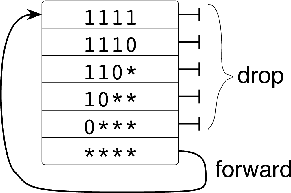
We first give a toy example of forwarding loop problem where the predicate filter of each rule is given by a wildcard expression, that is an -letter string in . Such an expression represents the set all -bit headers obtained by replacing each of the expression by either or . A packet with header in that set is said to match the rule. Figure 1 illustrates a one node network with wildcard expressions of letters. Rules are tested from top to bottom. All rules indicate to drop packets except the last one that forwards packets to the node itself. This network contains a forwarding loop if there exists a header that matches no rule except the last one. Not matching a rule as corresponds to having , , or . This one node network thus has a forwarding loop iff the formula is satisfiable, which is not the case. This simple example can easily be generalized to reduce SAT to forwarding loop detection in networks with wildcard rules. It also points out a key problem: testing the emptiness of expressions such as where are the sets associated to rules.
As packet headers in practical networks such as Internet typically have hundreds of bits, search of the header space is completely out of reach. The main challenge for solving such a problem thus resides in limiting the number of tests to perform. For that purpose, previous works [17, 15] propose to consider sets of headers that match some predicate filters and do not match some others. Defining two headers as equivalent when they match exactly the same predicate filters, it then suffices to perform one test per equivalence class. These classes are indeed the atoms (the minimal non-empty sets) of the field of sets (the (finite) -algebra) generated by the sets associated to the rules.
A first challenge lies in efficiently identifying and representing these atoms. This would be fairly easy if both intersection and complement could be represented efficiently. In practice, most classical compact data-structures for sets of bit strings are closed under intersection but not under complement. For example, the intersection of two wildcard expressions, if not empty, can obviously be represented by a wildcard expression, but the complement of a wildcard expression is more problematic. Previous works overcome this difficulty by representing the complement of a -letter wildcard expression as the union of several wildcard expressions (up to ). However, this can result in exponential blow-up and the tractability of these methods rely on various heuristics that do not offer rigorously proven guarantees.
A second challenge lies in understanding the tractability of practical networks. One can easily design a collection of wildcard expressions that generates all the possible singletons as atoms (all the -letters strings with only one non- letter). What does prevent such phenomenon in practice? Can we provide a property that intuitively fits with practical network and guarantees that the number of atoms does not blow up? This paper aims at addressing both challenges with provable guarantees.
Related work
The interest for network problem diagnosis has recently grown after the advent of Software-Defined Networking (SDN) [23, 18, 21, 12]. SDN offers the opportunity to manage the forwarding tables of a network with a centralized controller where full knowledge is available for analysis. Previous works has led to a series of methods for network analysis, resulting in several tools [17, 13, 19, 27]. The main approaches rely on computing classes of headers by combining rule predicate filters using intersection and set difference (that is intersection with complement). The idea of considering all header classes generated by the global collection of the sets associated to all forwarding rules in the network is due to Veriflow [17]. However, the use of set differences results in computing a refined partition of the atoms of the field of sets generated by this collection that can be much larger than an exact representation. NetPlumber [13], which relies on the header space analysis introduced in [15], refines this approach by considering the set of headers that can follow a given path of the network topology. This set is represented as a union of classes that match some rules (those that indicate to forward along the path) and not some others (those that have higher priority and deviate from the path): a similar problem of atom representation thus arises. The idea of avoiding complement operations is somehow approached in the optimization called “lazy subtraction” that consists in delaying as much as possible the computation of set differences. However, when a loop is detected, formal expressions with set differences have to be tested for emptiness. They are then actually developed, possibly resulting in the manipulation of expressions with exponentially many terms.
Concerning the tractability of the problem, the authors of NetPlumber observe a phenomenon called “linear fragmentation” [15, 14] that allows to argue for the efficiency of the method. They introduce a parameter measuring this linear fragmentation and claim a polynomial time bound for loop detection for low [15] (when emptiness tests are not included in the analysis). However, the rigorous analysis provided in [14] includes a factor where is the diameter of the network graph. While this factor appears to be largely overestimated in practice, the sole hypothesis of linear fragmentation does not suffice for explaining tractability and prove polynomial time guarantees. The alternative approach of Veriflow is specifically optimized for rules resulting from range matching within each field of the header. When the number of fields is constant, polynomial time execution can be guaranteed but this result does not extend to general wildcard matching.
A similar problem consists in conflict detection between rules and their resolution [1, 9, 5]. It has mainly been studied in the context of multi-range rules [1, 9], which can benefit from computational geometry algorithms. (A multi-range can be seen as a hyperrectangle in a -dimensional euclidean space where is the number of fields composing headers.) Another similar problem, determining efficiently the rule that applies to a given packet, has been studied for multi-ranges [9, 10, 11]. In the case of wildcard matching, such problems are related to the old problem of partial matching [24]. It is believed to suffer from the “curse of dimensionality” [3, 22] and no method significantly faster than exhaustive search is expected to be found with near linear memory (although some tradeoffs are known for small number of letters [7]). However, efficient hardware-based implementations exist based on Ternary Content Addressable Memory (TCAMs) [4] or Graphics Processing Unit (GPU) [26].
Regarding the manipulation of set collections, recent work [20] shows how to enumerate all sets obtained by closure under given set operations with polynomial delay. In particular, this allows to produce the field of sets generated by the collection. However, this setting requires a set representation which explicitly lists all elements and does not apply here. Another issue comes from the fact that the field set can be exponentially larger than its number of atoms.
Our contributions
First, we make a key algorithmic step by providing an efficient algorithm for computing an exact representation of the atoms of the field of sets generated by a collection of sets. The representation obtained is linear in the number of atoms and allows to test efficiently if an atom is included in a given set of the collection. The main idea is to represent an atom by the intersection of the sets that contain it. We avoid complement computations by using cardinality computations for testing emptiness. Our algorithm is generic and supports any data-structure for representing sets of -bit strings that supports intersection and cardinality computation in bounded time for some value . It runs in polynomial time with respect to , the number of sets and atoms respectively. Beyond combinations of wildcard and range expressions, we believe that it could be extended to support expressions on hashed values (for a fixed hash function) or bloom filters by defining auxiliary cardinality measures.
| Rule repr. | Trivial | NetPlumber [13] | Veriflow [17] | This paper |
| -bounded | – | – | ||
| ” ov. deg. | ” | – | – | |
| ” ov. deg. | ” | – | – | |
| -wildcard | ||||
| ” ov. deg. | ” | |||
| -multi-rng. | – | |||
| ” ov. deg. | ” | – |
Second, we provide a dimension parameter, the overlapping degree , that captures the complexity of a collection of rule sets considered in a forwarding network. It is defined as the maximum number of distinct rules (i.e. with pairwise distinct associated sets) that match a given header. This parameter constitutes a measure of complexity for the field of sets generated by a given collection of sets. In the context of practical hierarchical networks, we have the following intuitive reason to believe that this parameter is low: in such networks, more specific rules are used at lower levels of the hierarchy. We can thus expect that the overlapping degree is bounded by the number of layers of the hierarchy. Empirically, we observed a value within for datasets with hundreds to thousands of distinct multi-field rules, and for the collection of IPv4 prefixes advertised in BGP. A constant overlapping degree implies that the number of header classes is polynomially bounded, giving a hint on why practical networks are tractable despite the NP-completeness of the problem. In addition, the algorithm we propose is tailored to take advantage of low overlapping degree , even without knowledge of . Table 1 provides a summary of the complexity results obtained for loop detection depending on how the sets associated to rules are represented. Our techniques can be extended to handle write actions (partial writes of fixed values such as field replacement) while maintaining polynomial guarantees.
Our algorithm for atom computation solves two difficult technical issues. First, it manages to remain polynomial in the number of atoms even though the number of sets generated by intersection solely can be exponential in with general rules. Second, the use of cardinality computations allows to avoid exponential blow-up (in contrast with previous work) but naturally induces a quadratic term in the complexity. However, we manage to reduce it to in the case of collections with logarithmic overlapping degree (i.e. ). Indeed, our algorithm then becomes linear in and polynomial in , providing an algorithmic breakthrough towards efficient atom enumeration.
Roadmap: Section 2 introduces the model. Section 3 describes how to represent the atoms of a field of sets. We state in Section 4 our main result concerning atom computation and its implications for forwarding loop detection that give the upper bounds listed in Table 1. Section 5 gives more insight about the comparison of our results with previous works and justifies the lower bounds presented in Table 1. Finally, Section 6 discusses some perspectives.
2 Model
2.1 Problem
We consider a general model of network where a network instance is characterized by:
-
a graph where each node is a router and has a forwarding table .
-
a natural number representing the (fixed) bit-length of packet headers.
Let denote the set of all possible headers (all -bit strings). Each forwarding table is an ordered list of forwarding rules . Each forwarding rule , is made of a predicate filter and an action to apply on any packet whose header matches the predicate. We say that a header matches rule when it matches predicate (we may equivalently say that matches ). We then write to emphasize the fact that can be viewed as a compact data-structure encoding the set of headers that match it. This set is called the rule set associated to . For the ease of notation, we thus let denote both the predicated filter of rule and the associated set.
We consider three possible actions for a packet: forward to a neighbor, drop, or deliver (when the packet has reached destination). The priority of rules is given by their ordering: when a packet with header arrives at node , the first rule matched by is applied. Equivalently, the rule is applied when , where denotes the complement of . When no match is found (i.e. ), the packet is dropped.
Given a header , the forwarding graph of represents the forwarding actions taken on a packet with header : when the first rule that matches in indicates to forward to . The forwarding loop detection problem consists in deciding whether there exists a header such that has a directed cycle.
Note that we make the simplifying assumption that the input port of an incoming packet is not taken into account in the forwarding decision of a node. In a more general setting, a node has a forwarding table for each incoming link. This is essentially the same model except that we consider the line-graph of instead of .
2.2 Header Classes
A natural relation of equivalency exists between headers with respect to rules: two headers are equivalent if they match exactly the same rules, that is if they belong to the same rule sets. Trivially, two equivalent headers let the corresponding packets have exactly the same behavior in the network. The resulting equivalence classes partitions the header set into nonempty disjoint subsets called header classes. To check any property of the network, it suffices to do it on a class-by-class basis instead of a header-by-header basis. The number of header classes is thus a natural parameter when considering the difficulty of forwarding loop detection (or other similar network analysis problems). A more accurate definition of classes could take into account the order of rules and the topology (see Appendix E) but this does not allows us to obtain complexity gain in general.
The header classes can be defined according to the collection of rule sets of (i.e. ). If denotes the set of all rule sets associated to the rules matched by a given header , then its header class is clearly equal to (with the convention ). Such sets are the atoms of the field of sets generated by . Their computation is the main topic of this paper and is detailed in the next section.
2.3 Set representation
As we focus on the collection of rule sets, we now detail our hypothesis on their representation. We assume that a data-structure allows to represent some of the subsets of a space . For the ease of notation, also denotes the collection of subsets that can be represented with . We assume that is closed under intersection: if and are in , so is . We say that such a data-structure for subsets of is -bounded when intersection and cardinality can be computed in time at most: given the representation of , the representation of and the size of (as a binary big integer) can be computed within time . As big integers computed within time have bits, this implies : the bound obviously depends on . Intersection, inclusion test (), cardinality computation () and cardinality operations (addition, subtraction and comparison) are called elementary set operations. Under the -bounded hypothesis, all these operations can be performed in time ( is equivalent to ).
Two typical examples of data-structures meeting the above requirements are wildcard expressions and multi-ranges. In a forwarding network, we consider the header space of all -bit strings, which may be decomposed in several fields. A rule set is typically represented by a wildcard expression or a range of integers. In both cases, they can be represented within bits and both representation are -bounded. We call -wildcard a string . It represents the set . If rules are decomposed into fields, any combinations of wildcard expressions and ranges can be used (either one for each field) and represented within bits. However cardinality computations can take time as multiplications of big integers are required. Such representation is thus -bounded. Given field lengths with sum , we call -multi-range a cartesian product of integer ranges with for in . It represents the set where is the binary representation of within bits.
When manipulating a collection of sets in , we assume that their representations are stored in a balanced binary search tree, allowing to dynamically add, remove or test membership of a set in time. More efficient data-structures (tries and segment trees) can be used for wildcard expressions and multi-ranges as detailed in Appendix A.1.
3 Atoms and combinations generated by a collection of sets
Given a space of elements , a collection is a finite set of subsets of . The field of sets generated by a collection is the (finite) -algebra generated by , that is the smallest collection closed under intersection, union and complement that contains .
The atoms of are classically defined as the non-empty elements that are minimal for inclusion. For brevity, we call them the atoms generated by . Let denote their collection. Note that for and , we have either or (otherwise and would be non-empty elements of strictly included in ). This gives a characterization of the atoms that matches our definition of header classes when is the collection of rule sets of a network (see Section 2.2):
| (1) |
For example, the collection pictured in Figure 2 generates 7 atoms: , , , , , , and .
Due to the complement operations, the atoms can be harder to represent than the rules they are generated from. In Figure 2, all rules are ranges, but the atom is not. When the intersection operation can be computed and represented efficiently (see Section 2.3), it is natural to consider the collection of combinations defined as sets that can obtain by intersection from sets in :
| (2) |
In Figure 2, there are 8 combinations: , , , , , , and .
Given a collection and a subset , we let denote the of , that is the sets in that contain . We associate each combination with the set . The function (with parenthesis) should not be confused with an atom (without parenthesis). A combination is said to be covered if (the union of its non-containers covers it), otherwise it is uncovered. Similarly, we associate each atom with the combination (this corresponds to the “positive” part of the characterization from Equation 1). The following proposition states that atoms can be represented by uncovered combinations.
Proposition 1.
The collection of uncovered combinations is in one-to-one correspondence with the atom collection : each corresponds to the atom . Reciprocally, each atom is mapped to combination .
Based on Proposition 1, we say that an uncovered combination represents atom . can be seen as a canonical representation of by a collection of combinations. In Figure Figure 2, atom is represented by combination . Similarly, atoms , , , , and are represented by (uncovered) combinations , , , , , and respectively. Combination is covered: .
The proof of Proposition 1 is straightforward. First, we verify that if is an uncovered combination, is an atom: it suffices to observe that and to match with the atom characterization given by Equation 1 using . Similarly, if is an atom for some , the combination satisfies which implies . In particular, as , is uncovered.
A nice property of the characterization of Proposition 1 is that it allows to efficiently test whether a set contains an atom : given a combination that represents , is equivalent to . This comes from the fact that every uncovered combination has same containers as . (If it was not the case, and is covered.) This explains the importance of determining , and in particular to separate covered combinations from uncovered ones. This is the subject of the next section, but we first formally introduce the notion of overlapping degree.
Overlapping degree of a collection
Our representation is naturally associated to the following measure of complexity of a collection . We define the overlapping degree of as the maximum number of containers of an element, that is . Note that all elements within an atom have same containers in and that a set cannot have more containers than any of its elements. We thus have:
As any atom can be expressed as where is the set of containers of , the number of atoms is obviously bounded by where denotes the number of sets in . The overlapping degree of a collection thus measures its complexity in terms of number of atoms it may generate.
We similarly define the average overlapping degree as the average number of containers of an atom: . We obviously have . Given a collection , we will also consider the average overlapping degree of combinations, that is the average overlapping degree of . Note that has the same collection of atoms as and that a combination containing an atom must satisfy . The overlapping degree of is thus at most and we always have .
In the example from Figure 2, one can verify that we have , and .
4 Incremental computation of atoms
We can now state our main result concerning the computation of the atoms generated by a collection of sets.
Theorem 1.
Given a space set and a collection of subsets of , the collection of combinations that canonically represent the atoms can be incrementally computed with elementary set operations where: is the number of atoms generated by ; is the overlapping degree of ; is the average overlapping degree of ; is the average overlapping degree of . Within this computation, each combination can be associated to the list of sets in that contain . If sets are represented by -wildcard expressions (resp. -multi-ranges), the representation can be computed in (resp. ) time.
Application to forwarding loop detection
Theorem 1 has the following consequences for forwarding loop detection.
Corollary 1.
Given a network with collection of rule sets with -bounded representation, forwarding loop detection can be performed in time where is the number of atoms in , is the overlapping degree of and (resp. ) is the average overlapping degree of (resp. ). If sets are represented by -wildcard expressions (resp. -multi-ranges), the representation can be computed in (resp. ) time.
This result can be extended to handle write actions as explained in Appendix F due to the lack of space. The upper-bounds for forwarding loop detection listed in Table 1 follow from Corollary 1 which is proved in Appendix A.3. A key ingredient consists in maintaining for each rule set a list that describes its presence, priority and action for each node. Detecting a loop for a header class then consists in merging the lists associated to the rule sets containing (as provided by our atom representation) for obtaining the forwarding graph for all . Directed cycle detection is finally performed on each such graph.
In the rest of this Section, we prove Theorem 1 by introducing two incremental algorithms for atom computation and analyzing their performance. The incremental approach allows to avoid exponential blow-up even in cases where the number of combinations can be exponential in the number of atoms (an example is given in Appendix B.2).
Algorithms for updating atoms
We first propose a basic algorithm for updating the collection of uncovered combinations of a collection when a set is added to . The main idea is that after adding to , the only new uncovered combinations that can be created are intersections of pre-existing uncovered combinations with (see Lemma 1 in Appendix A.2). We thus first add to the combinations for . As this may introduce covered combinations, we then compute the atom size for each combination . It is then sufficient to remove any combination with to finally obtain . This atom size computation is possible because we have for all . (see Lemma 2 in Appendix A.2). As this union is disjoint, we have . We thus compute the inclusion relation between combinations and store in the combinations that strictly contain . Initializing to for all , we then scan all combinations by non-decreasing cardinality (or any topological order for inclusion) and subtract from for each . A simple proof by induction allows to prove that when is scanned. The whole process in summarized in Algorithm 1.
The correctness of Algorithm 1 follows from the two above remarks (that is Lemma 1 and Lemma 2 in Appendix A.2). Its main complexity cost comes from intersecting with each combination and computing the inclusion relation between combinations, that is and elementary set operations respectively. Starting from and incrementally applying Algorithm 1 to each set in thus allows to obtain with elementary set operations, yielding the general bound of Theorem 1.
To derive better bounds for low overlapping degree , we propose a more involved algorithm that maintains and from one iteration to another and makes only the necessary updates. This requires to handle several subtleties to enable lower complexity.
We similarly start by computing the collection of combinations intersecting . A first subtlety comes from the fact that several combinations may result in the same . However, we are only interested in the combination which is minimal for inclusion that we call the parent of . The reason is that can then be computed from . The parent is unique unless is covered in which case is marked as covered and discarded (see the argument for computation later on). To obtain right parent information, we thus process all by non-decreasing cardinality. The produced combinations such were not in are called new combinations. Their atom size is initialized to . See the “Parent computation” part of Algorithm 2.
We then remark that we only need to compute (or update) for combinations that include , which we store in a set Incl. We also note that needs to be computed when is new and updated when is the parent of a new combination. A second subtlety resides in computing (or updating) only when is not covered that is when (after computation) appears to be non-zero. As the computation of lists is the most heavy part of the computation, this is necessary to enable our complexity analysis. For that purpose, we scan Incl by non-decreasing cardinality so that the correct value of is known when is scanned similarly as in Algorithm 1. However, we avoid any useless computation when is zero. Otherwise, we compute (or update) and decrease by from for adequate : if and where both in , this computation has already been made; it is only necessary when is new or when is the parent of . We optionally maintain for each combination a list that contain the list of sets that contain (Such lists are not necessary for the computation but they are useful for loop detection as detailed in Appendix A.3). See the “Atom size computation” part of Algorithm 2.
A last critical point resides in the computation of for each new combination . The list can be obtained from by copying and also intersecting elements of with . This is sufficient: for such that , we can consider . If , by minimality of and we thus have . The case where and cannot happen as it would imply that two different combinations and generate by intersection with () and are both minimal for inclusion. In such case, was covered in and so would be in (and also in ). That is why such combination are already discarded during parent computation. On the other hand, the list of a combination can be updated by intersecting elements of with : when for , we have .
Finally, combinations with are discarded and removed from list of remaining combinations as detailed in the “Remove covered combinations” part of Algorithm 2.
The main argument in the complexity analyzis of Algorithm 2 comes from bounding the size of each list by (this is where the overlapping degree of is used). The number of elementary set operations performed is indeed where denotes the number of atoms of , denotes the atoms of included in , and denotes the uncovered combinations of that contain . A key step consists in proving . The accounts for membership tests and add/remove operations on collections of combinations. In the case of -wildcard and -multi-ranges, this factor can be saved by storing collections of sets in tries rather than balanced binary search trees. With -multi-ranges, a segment tree allows to retrieve Inter in elementary set operations [2, 8].
The various bounds for low overlapping degree of Theorem 1 results from applying iteratively Algorithm 2 for each set of and by carefully bounding the sums of terms. Intuitively, each atom generated by the collection of the first sets of can be associated to an atom of such that where . As each atom is included in sets of at most, this allows to bound the overall sum of terms by . Details are given in Appendix A.2.
5 Comparison with previous works
We give in Appendix C more details about “linear fragmentation”, a phenomenon observed by Kazemian et al. [14], and propose small overlap degree as a plausible cause. The notion of uncovered combination is linked to that of weak completion introduced by [5] in the context of rule-conflict resolution as detailed in Appendix D. We now provide examples where use of set complement computation can lead to exponential blow-up in previous work.
5.1 Veriflow
Veriflow [17] incrementally computes a partition into sub-classes that forms a refinement of the header classes: when a rule is added, each sub-class is replaced by and a partition of . Veriflow benefits from the hypothesis that headers can be decomposed into fixed fields and that each rule set can be represented by a multi-range . The intersection of two multi-ranges is obviously a multi-range. However, set difference is obtained by intersection with the complement which is represented as the union of up to multi-ranges. We prove in Appendix B.1 that successive difference with rules of the form with can generate multi-ranges in the computations of Veriflow as indicated in Table 1.
5.2 HSA / NetPlumber
HSA/NetPlumber [15, 13] use clever heuristics to efficiently compute the set of headers than can traverse a given path . An important one consists in lazy subtraction: set difference computations are postponed until the end of the path. For that purpose, this set is represented as a union of terms of the form where the elementary sets are represented with wildcards. The emptiness of such terms is regularly tested. A simple heuristic is used during the construction of the path: is obviously empty if is included in for some . But if the path loops, HSA has to develop the corresponding terms into a union of wildcards to determine if one of them may produce a forwarding loop.
We now provide an example where this emptiness test can take exponential time. Consider a node whose forwarding table consists in rules with following rule sets:
All rules are associated with the drop action except the last rule (with rule set ) whose action is to forward to the node itself. Such a forwarding table is depicted in Figure 1 for . Starting a loop detection from that node, HSA detects a loop for headers in . The emptiness of this term is thus tested. For that purpose, HSA represents the complement of with . Note that each of the wildcard expressions in that union have only one non- letter. Distributivity is then used to compute as . After expanding the first intersections, HSA thus obtains a union of wildcards with letters in and letters equal to that has to be intersected with . In particular, this unions contains all strings with letters equal to and equal to . All -letter strings with alphabet are produced during the computation which thus requires time. For testing a network with similar nodes, HSA thus requires time . As all sets are pairwise disjoint, the overlapping degree of the collection is and this justifies the two lower-bounds indicated for NetPlumber in Table 1.
6 Future work
Our approach could be naturally integrated in the Veriflow [17] framework both for speed-up and performance-guarantee considerations. Our ideas can also be integrated in the NetPlumber [13] framework (see the similar approach proposed in Appendix E). This would allow to enhance the emptiness tests performed within NetPlumber to guarantee polynomial time execution when the number of header classes is polynomially bounded. In the context of multi-ranges, the emptiness test of expressions is equivalent to the Klee measure problem which consists in computing the volume of a union of boxes. Indeed, expression is empty when the volume of the union of the boxes equals that of . According to recent work [6], the complexity of this problem is believed to be . It would be interesting to determine if such low complexity bounds extend to atom computation in the case of multi-ranges rules.
References
- [1] Hari Adiseshu, Subhash Suri, and Guru M. Parulkar. Detecting and resolving packet filter conflicts. In Proceedings IEEE INFOCOM 2000, The Conference on Computer Communications, Nineteenth Annual Joint Conference of the IEEE Computer and Communications Societies, Reaching the Promised Land of Communications, Tel Aviv, Israel, March 26-30, 2000, pages 1203–1212. IEEE, 2000.
- [2] Mark de Berg, Otfried Cheong, Marc van Kreveld, and Mark Overmars. Computational Geometry: Algorithms and Applications. Springer-Verlag TELOS, Santa Clara, CA, USA, 3rd ed. edition, 2008.
- [3] Allan Borodin, Rafail Ostrovsky, and Yuval Rabani. Lower bounds for high dimensional nearest neighbor search and related problems. In Jeffrey Scott Vitter, Lawrence L. Larmore, and Frank Thomson Leighton, editors, Proceedings of the Thirty-First Annual ACM Symposium on Theory of Computing, May 1-4, 1999, Atlanta, Georgia, USA, pages 312–321. ACM, 1999.
- [4] Pat Bosshart, Glen Gibb, Hun-Seok Kim, George Varghese, Nick McKeown, Martin Izzard, Fernando Mujica, and Mark Horowitz. Forwarding metamorphosis: Fast programmable match-action processing in hardware for SDN. In Proceedings of the ACM SIGCOMM 2013 Conference on SIGCOMM, SIGCOMM ’13, pages 99–110, New York, NY, USA, 2013. ACM.
- [5] Matthieu Boutier and Juliusz Chroboczek. Source-specific routing. In IFIP Networking, 2015.
- [6] Timothy M. Chan. Klee’s measure problem made easy. In 54th Annual IEEE Symposium on Foundations of Computer Science, FOCS 2013, 26-29 October, 2013, Berkeley, CA, USA, pages 410–419. IEEE Computer Society, 2013.
- [7] Moses Charikar, Piotr Indyk, and Rina Panigrahy. New algorithms for subset query, partial match, orthogonal range searching, and related problems. In Peter Widmayer, Francisco Triguero Ruiz, Rafael Morales Bueno, Matthew Hennessy, Stephan Eidenbenz, and Ricardo Conejo, editors, Automata, Languages and Programming, 29th International Colloquium, ICALP 2002, Malaga, Spain, July 8-13, 2002, Proceedings, volume 2380 of Lecture Notes in Computer Science, pages 451–462. Springer, 2002.
- [8] Herbert Edelsbrunner and Hermann A. Maurer. On the intersection of orthogonal objects. Information Processing Letters, 13(4):177–181, 1981.
- [9] David Eppstein and S. Muthukrishnan. Internet packet filter management and rectangle geometry. In S. Rao Kosaraju, editor, Proceedings of the Twelfth Annual Symposium on Discrete Algorithms, January 7-9, 2001, Washington, DC, USA., pages 827–835. ACM/SIAM, 2001.
- [10] Anja Feldmann and S. Muthukrishnan. Tradeoffs for packet classification. In Proceedings IEEE INFOCOM 2000, The Conference on Computer Communications, Nineteenth Annual Joint Conference of the IEEE Computer and Communications Societies, Reaching the Promised Land of Communications, Tel Aviv, Israel, March 26-30, 2000, pages 1193–1202. IEEE, 2000.
- [11] Pankaj Gupta and Nick McKeown. Algorithms for packet classification. IEEE Network: The Magazine of Global Internetworking, 15(2):24–32, March 2001.
- [12] Naga Praveen Katta, Jennifer Rexford, and David Walker. Incremental consistent updates. In Proceedings of the Second ACM SIGCOMM Workshop on Hot Topics in Software Defined Networking, HotSDN ’13, pages 49–54, New York, NY, USA, 2013. ACM.
- [13] Peyman Kazemian, Michael Chang, Hongyi Zeng, George Varghese, Nick Mckeown, Scott Whyte, and U C San Diego. Real Time Network Policy Checking using Header Space Analysis. In NSDI, 2013.
- [14] Peyman Kazemian, George Varghese, and Nick McKeown. Header space analysis: Static checking for networks. Technical report, Stanford, 2011. http://yuba.stanford.edu/ peyman/docs/headerspace_tech_report.pdf.
- [15] Peyman Kazemian, George Varghese, and Nick McKeown. Header space analysis: Static checking for networks. In Presented as part of the 9th USENIX Symposium on Networked Systems Design and Implementation (NSDI 12), pages 113–126, San Jose, CA, 2012. USENIX.
- [16] Kazemian Peyman. HSA/NetPlumber source code repository. https://bitbucket.org/peymank/hassel-public/.
- [17] Ahmed Khurshid, Xuan Zou, Wenxuan Zhou, Matthew Caesar, and P Brighten Godfrey. VeriFlow : Verifying Network-Wide Invariants in Real Time. In NSDI, 2013.
- [18] Vasileios Kotronis, Xenofontas Dimitropoulos, and Bernhard Ager. Outsourcing the routing control logic: Better internet routing based on SDN principles. In Proceedings of the 11th ACM Workshop on Hot Topics in Networks, HotNets-XI, pages 55–60, New York, NY, USA, 2012. ACM.
- [19] Haohui Mai, Ahmed Khurshid, P Brighten Godfrey, and Samuel T King. Debugging the Data Plane with Anteater. In SIGCOMM, 2011.
- [20] Arnaud Mary and Yann Strozecki. Efficient enumeration of solutions produced by closure operations. In Nicolas Ollinger and Heribert Vollmer, editors, 33rd Symposium on Theoretical Aspects of Computer Science, STACS 2016, February 17-20, 2016, Orléans, France, volume 47 of LIPIcs, pages 52:1–52:13. Schloss Dagstuhl - Leibniz-Zentrum fuer Informatik, 2016.
- [21] Christopher Monsanto, Joshua Reich, Nate Foster, Jennifer Rexford, and David Walker. Composing software-defined networks. In Proceedings of the 10th USENIX Conference on Networked Systems Design and Implementation, nsdi’13, pages 1–14, Berkeley, CA, USA, 2013. USENIX Association.
- [22] Mihai Patrascu. Unifying the landscape of cell-probe lower bounds. SIAM J. Comput., 40(3):827–847, 2011.
- [23] Peter Perešíni, Maciej Kuzniar, Nedeljko Vasić, Marco Canini, and Dejan Kostic. OF.CPP: Consistent Packet Processing for Openflow. In Proceedings of the Second ACM SIGCOMM Workshop on Hot Topics in Software Defined Networking, HotSDN ’13, pages 97–102, New York, NY, USA, 2013. ACM.
- [24] Ronald L. Rivest. Partial-match retrieval algorithms. SIAM J. Comput., 5(1):19–50, 1976.
- [25] Route Views Project. BGP traces. http://routeviews.org/.
- [26] Matteo Varvello, Rafael Laufer, Feixiong Zhang, and T.V. Lakshman. Multi-layer packet classification with graphics processing units. In CoNEXT, 2014.
- [27] Hongyi Zeng, Shidong Zhang, Fei Ye, Vimalkumar Jeyakumar, Mickey Ju, Junda Liu, Nick McKeown, and Amin Vahdat. Libra: Divide and conquer to verify forwarding tables in huge networks. In Proceedings of the 11th USENIX Conference on Networked Systems Design and Implementation, NSDI’14, pages 87–99, Berkeley, CA, USA, 2014. USENIX Association.
Appendix A : Proof details of Theorem 1 and Corollary 1
We present here a refined version of Theorem 1 with more hypothesis about the data-structure used to store a collection of sets. We first review these hypothesis and then the proof details of both versions.
A.1 Collection of sets representation
When manipulating a collection of sets in , we assume that their representations are stored in a collection data-structure allowing to dynamically add, remove or test membership of a set. Such operation are called -collection operations. We can use a balanced binary search tree when comparisons according to a total order can be performed. Such comparison can usually be obtained by comparing directly the binary representations themselves of the set in linear time (and thus for sets with -bounded representation). It is considered as an elementary set operation. In the case of wildcard expressions, the complexity of these operations can be reduced to time by using a trie or a Patricia tree. Our algorithms will also make use of an operation similar to stabbing query that we call -intersection query. It consists in producing the list of sets in a collection of sets that intersect a given query set (). We additionally require that the list is topologically sorted according to inclusion. We say that -intersection queries can be answered with overhead when dynamically adding or removing a set from the collection takes time at most and the -intersection query for any set takes time at most. In the case of -dimensional multi-ranges, a segment tree allows to answer -intersection queries with overhead [2, 8]. In the case of wildcard expressions, a trie or a Patricia tree allows to answer -intersection queries with overhead (the whole tree has to be traversed in the worse case, but no sorting is necessary as the result is naturally obtained according to lexicographic order).
A.2 Incremental computation of atoms (Theorem 1)
The following is a refinement of Theorem 1 with respect to data-structures that provide time bounds on -collection operations and -intersection queries. For the sake of simplicity of asymptotic expressions, we make the very loose assumption that and . (We are mainly interested in the case where is large. Note also that examples with would be very peculiar.)
Theorem 2.
Given a space set and a collection of subsets of , the collection of combinations that canonically represent the atoms generated by can be incrementally computed with elementary set operations where denotes the number of atoms generated by , denotes the overlapping degree of , denotes the average overlapping degree of and denotes the average overlapping degree of .
More precisely, if the data-structures used for representing sets and collections of sets enable elementary set operations within time , -collection operations within time and -intersection queries with overhead , then the representation of the atoms generated by can be computed in time.
The following lemma formally states that uncovered combinations of can be obtained from and justifies the overall approach of Algorithm 2.
Lemma 1.
Given a new rule , the collection of uncovered combinations of can be obtained by intersecting uncovered combinations in with . More precisely, we have .
Proof.
Consider an uncovered combination . Let be the intersection of the containers of in : . We have either if or if . To conclude, it is thus sufficient to show that is uncovered in . This follows from and : the non-containers of in are also non-containers of in and if was covered, so would be . ∎
The following Lemma, which expresses any combination as a disjoint union of atoms justify the computation of atom cardinalities in Algorithm 2 by scanning lists for .
Lemma 2.
Given a combination collection containing , we have for all . This union is disjoint and we have .
Proof.
Reminding that any combination includes , we have . Conversely, consider . The sets of containing are , and we have for . As (the sets that contain also contain ) and , we have . Hence . This union is disjoint as each is either an atom or is empty. ∎
We can now state the following proposition about the guarantees of Algorithm 2.
Proposition 2.
Algorithm 2 allow to dynamically update the collection of uncovered combinations of a collection using elementary set operations when a rule is added to , where denotes the number of atoms of , denotes the atoms of included in , and denotes the uncovered combinations of that contain .
More precisely, if the data-structures used for representing sets and collections of sets enable elementary set operations within time , -collection operations within time and -intersection queries with overhead , then the update of can be performed in time.
Proof.
As discussed before the correctness of Algorithm 2 for obtaining uncovered combinations after adding set to a collection from and results from Lemma 1. For a new combination , the list is obtained from and is updated similarly for such that . The correctness of this approach has already been discussed in Subsection 4. We develop here the key argument for ignoring a combination when it is produced by several minimal elements such that for in . If this happens, we know that is not in , meaning that it is covered in and so is in . We can thus safely eliminate in the first phase of the algorithm. For the remaining new combinations , the parent of is the unique combination such that and which is minimal for inclusion.
The correctness of the atom cardinality computation follows by induction on the number combinations in Incl processed so far in the corresponding for loop. Consider a newly created combination . The initial value of is . Assuming that the correct value has been obtained for processed before and , has been subtracted from and Lemma 2 implies that when we consider in the for loop. For already in before adding and for processed before , has been subtracted from only for newly created . For , may have decreased but this difference is compensated by . This is the reason why Algoritihm 2 updates only besides such that . The correctness of the atom cardinality computation implies that all covered combinations are removed and the correctness of Algorithm 2 follows.
We now analyze the complexity of Algorithm 2. The bound in terms of elementary set operations is obtained when balanced binary search tree (BST for short) are used to store the various collections of sets (i.e. , Incl, New and for ). When adding a set , finding the combinations in that intersect is a -intersection query and can be performed in time or set operations using BST (sorting is only necessary in that case). The collection Incl is then constructed in operations with BST or with appropriate data-structures. Removing combinations such that is just a matter of scanning Incl again and can be done within the same complexity. Let denote the combinations included in Incl at that point (just before cardinality computations). The computation of for is done only when , i.e. only if represents one of the atoms in . we thus have . This requires at most operations. Note that for each uncovered combination yields at least one uncovered combination in ( itself or or both). We thus have . The overall computation of lists can thus be performed within set operations with BST and time with appropriate data-structures. The computation of class cardinalities and the removal of covered combinations from the lists have same complexity. Removal of covered combinations from and Incl takes collection operations and fits within the same complexity bound. Additional cost of is necessary when maintaining data-structures enabling efficient -intersection queries. The whole algorithm can thus be performed in time or using elementary set operations with BST.
To achieve the proof of complexity of Algorithm 2, we show . Consider a combination that intersects . Then can be associated to an atom of included in (such atoms exist according to Lemma 2). For any atom , let denote the atom in that contains (we have or ). Now for , consider the atom . As is an atom and is a combination intersecting , we have and is one of the combinations in that contains . For each such combination , intersects or (or both), and or is uncovered in . Both contain and we have . We can thus write . ∎
It should be noted that in the case of -multi-ranges, we can distinguish in the analysis, the computation of for new that costs from other cardinality manipulations (subtractions and comparisons) that take . This allows to obtain the bound claimed in Theorem 1.
Proof of Theorem 2.
From Proposition 2, the overall complexity of atom computation is
set operations where
denotes the number of atoms in
and denotes the
atoms of included in and
. We first consider the case where is
unbounded (it is possible to construct examples with and
). As we add a set to , the number of atoms can only
increase (each atom remains unchanged or is eventually split into two). We thus
have and .
Using , the overall complexity is
by definition of average overlap.
The bound is obtained by using Algortihm 1
instead of Algorithm 2.
We now derive a bound depending on the average overlapping degree of combinations. Consider an atom and an uncovered combination . We can associate to an atom in . As is also a combination in , we have where denotes the combinations of containing . As the atoms in are disjoint, the atoms for are pairwise distinct. We thus have . The overall complexity of atom computation is by definition of overlapping degree and average overlapping degree respectively. The refined bound in terms of is obtained similarly. ∎
A.3 Application to forwarding loop detection (Corollary 1)
Claim 1.
Given the collection of rule sets of a network , and for each atom the list of sets in that contain , forwarding loop detection can be solved in time where is the number of header classes, is the average overlapping degree of and is the number of nodes in .
Proof.
For that, we assume that each rule set is associated with the list of forwarding rules that have rule set . Each such rule is also supposed to be associated to the node whose table contains it and the index of the rule in . Each list is additionally supposed to be sorted according to associated nodes. Such lists can easily be obtained by sorting the collection of all forwarding tables according to the predicate filters of rules.
The claim comes from the fact that uncovered combination in represent atoms of . It follows from testing for each header class whether the graph for all has a directed cycle. is computed by merging the lists for in time . This graph has at most edges and cycle detection can be performed in time. The overall complexity follows from by definition of . ∎
Appendix B : Difficult inputs for previous works
B.1 Veriflow
Verfilow [17] represents the complementary of a multi-range as the union of multi-ranges (at most):
-
and ,
-
and ,
-
,
-
and ,
where denotes the maximum possible value in field , and denotes the multi-range of all possible values for fields for .
The difficult input for Veriflow consists in a network with rules associated to the following multi-ranges:
-
,
-
for .
Consider the sub-classes generated while computing . The union of multi-ranges representing contains in particular and . This implies that Veriflow generates on such an input all sub-classes of the form with for some (we set ). Forwarding loop detection of an -node network thus requires time for Veriflow. As this example has overlappingd degree 2, this justifies the two lower-bounds indicated for Veriflow in Table 1 for -multi-ranges.
It is possible to adapt Veriflow to support general wildcard matching by considering each field bit as a field. The wildcard expressions will then similarly generate all sub-classes obtained by concatenation of words and . This justifies the two lower-bounds indicated for Veriflow in Table 1 for -wildcards.
Appendix B.2 : HSA/NetPlumber approach
The NetPlumber approach could be generalized to more general types of rules. However, we show that the simple heuristic for emptiness tests described in Section 5.2 is not sufficient. We provide an example where the HSA/NetPlumber approach generates an exponential number of paths while the number of classes is linear if it relies solely on this heuristic. Consider header space and the following rule sets: and . Consider a network with nodes. Each node for and has table where action indicates to forward packets to node for and to drop packets for . Starting from , the HSA approach generates a path for each combination for and . This path goes through and then through . It is constructed at least for term . The heuristical emptiness test of NetPlumber does not detect that it is empty since contains for and it is not included in . The number of paths generated is thus at least . However, the header classes are all singletons of and their number is . Note the high overlapping degree of this collection of rule sets.
Appendix C : Linear fragmentation versus overlapping degree
Interestingly, a complexity analysis of HSA loop detection is given in the technical report [14] under an assumption called “linear fragmentation”. This assumption, which is based on empirical observations, basically states that there exists a constant such that a given routing path will branch at most times. More precisely it states that a term in the expression representing , the set of headers that can follow , intersects at most of the rule sets in the table of the end node of . A simple induction allows to bound the number of terms generated by all paths of hops from a given source by . Under linear-fragmentation, the time complexity of HSA loop detection (excluding emptiness tests) is thus proved to be in [14] where is the diameter of network graph , the number of rules, and the number of ports in (in our simplified model each node has a single input port and the number of nodes in ). It is then argued that in practice the constant gets smaller as the length of the path considered increases and that practical loop detection has complexity as claimed in [15]. However, it is not rigorous to neglect the (exponential) factor under the sole linear-fragmentation hypothesis.
Additionally, we think that low overlapping degree provides a simple explanation for the phenomenon observed by Kazemian et al.: as the path length increases, the terms representing the header that can traverse the path result from the intersection of more rules and become less likely to intersect other rules when overlapping degree is limited. Moreover, bounded overlapping degree implies that the number of terms generated by HSA within hops is bounded by . The total number of terms generated is thus bounded by . This guarantees that all HSA computations besides emptiness tests remain polynomial for constant . In contrast, with the example provided in Appendix B.2 (which has unbounded overlapping degree), the HSA approach can generate exponentially many paths compared to the number of header classes in the context of general rules.
Appendix D : Related notion of weak completeness
In the context of resolution of conflicts between rules, Boutier and Chroboczek [5] introduce the concept of weak completeness: a collection is weakly complete iff for any sets , we have . They show that this is a minimal necessary and sufficient condition for all rule conflicts to be solved when priority of rules extends inclusion (i.e. has priority over when ). Interestingly, we can make the following connection with this work: given a combination collection containing , we have for all . (See Lemma 2 in Appendix A.2.) This allows to show that is weakly complete. It is indeed the smallest collection of combinations of that contains and that is weakly complete. Our work thus also provides an algorithm for computing such an optimal “weak completion”.
Appendix E : Topological header classes
Inspired by the HSA/NetPlumber [15, 13] approach, we can refine the definition of header classes. We fix a source node . A forwarding path originating from is a sequence where are the nodes encountered along the path and are the indexes of the forwarding rules followed: rule is applied at node , then rule at node and so on. We then define two headers as topologically equivalent from if they follow the same forwarding paths. Note that each topological class for that relation corresponds to a unique path (if some headers match two distinct rules at a node, the first one is followed).
We now show that the topological classes (from ) are indeed certain atoms of partial collections of rule sets. Given a forwarding path . Let denote the collection of rule sets of node where corresponds to the order of the rules in . Let also denote the partial collection of the first rule sets. The set of headers that can follow rule in node is . If corresponds to a topological class , we have . As the only positive terms of this intersection are , is indeed the atom associated to the combination in . Note that we consider a different partial collection for each path. Our framework can thus be applied to test whether the combination associated to any path does correspond to a topological class by testing the emptiness of . We detect a forwarding loop (starting from ) as soon as a path reaches a former node of .
Our incremental algorithm is well suited for incrementally augmenting the collection of rules as we progress along the path. Using a persistent style implementation for the data structure storing collections (as classically done when implementing binary search trees in functional languages), we can step back at a branching node and follow a different branch without having to recompute the collection of atoms generated by the path up to . The collection is also incrementally augmenting as we progress in routing table of a branching node and explore different paths. This allows to efficiently perform a search of the graph in a depth first search manner.
It is important to note that two different explored paths and are associated to different combinations . To see this, suppose that and branch at node : follows rule of while follows with . After , path cannot follow any rule associated with set due to emptiness tests. This ensures that the number of paths generated is bounded. Similarly to the proof of Proposition 2 and Theorem 2, each combination generated by a path can be associated to an atom of where denotes the collection of all rule sets in the network. The number of topological classes is thus always bounded by . However, for a given collection of rule sets generating atoms, one can easily produce a network topology with topological classes.
When performing the search from source , the number of paths (and prefixes of paths) generated is at most where are the uncovered combinations generated by . As each path prefix accounts for one call of Algorithm 1, this search thus costs elementary set operations. Repeating this for all possible source nodes, we get an overall complexity of operations for forwarding loop detection. (This complexity analysis can be refined in terms of overlapping degree and optimized by using potentially Algorithm 2 instead of Algorithm 1.)
Note that the number of paths explored could grow exponentially without appropriate emptiness tests as exemplified in Appendix B.2. Although this approach remains polynomial in terms of and , its complexity guaranties are less interesting than what we propose in Section 4. However, it allows to extend our framework with write actions as detailed in the next appendix.
Appendix F : Write actions
First note that allowing any write operations and variable header length (by allowing to push sub-headers) make the forwarding loop detection problem undecidable as we can then easily simulate a pushdown automaton with several stacks. However, in the context of MPLS, it is natural to allow to push and pop MPLS headers (and only that type). In the classical functioning of MPLS, each push or swap action always writes a fixed label value, rules taking into account the MPLS header always have higher priority and base their decisions on the outermost label only (and no other field). In that case, paths with MPLS forwarding can be factored out by adding shortcut edges (from the first push action to last pop action) in a preliminary step which should also include loop detection for each label value pushed somewhere in the network. This can clearly be performed in polynomial time. We reserve the study of more general write action with push and pop actions for future work. However, we now sketch how to handle write actions in the context of fixed length headers.
We suppose that a forwarding rule applied to a packet can perform a write action before forwarding the packet. We typically think of write actions that write some fixed values at fixed positions. We then see a write action as a projection of the header space in a smaller sub-space. More generally, we assume that each write action is associated with a function with the following properties (we set for ) :
-
intersection preservation: for , we have ;
-
two consecutive write operations and are equivalent to a single write operation with , is then called a write pattern assumed to be efficiently computable.
We do not need to formally assume that is a projection (i.e. ) although this is typically the case.
We additionally make the following assumption with respect the data-structure used for sets:
-
is in and can be computed in time.
All the above requirements are clearly met for any write action (of fixed bits at fixed positions) in the context of wildcard expressions. In the context of prefix matching we can only allow to write a prefix of bits to ensure that a set represented by a prefix is always mapped to a set that can be represented by a prefix. We can generalize this to the context of interval matching when low order bits are ordered first (little-endian order). We still represent a set with an interval but we additionally consider a write pattern and the number of bits of written so far. The write pattern is simply an integer with same bit representation as and . To test whether a header is in , we first check that its lowest bits are identical to those of , then shift , , and by bits to erase low order bits, obtaining respectively and test whether . Other set operations are handled similarly. Note that the computation of just requires to update the write pattern which can be globally shared for a collection of sets. A similar trick can be used with wildcard expressions. In the context of multi-ranges, our model thus enables prefix writes on one or several fields. (This includes in particular writing of exact values in one or several fields.)
Forwarding loop detection can then be performed using the approach detailed in Appendix E by additionally decorating each node of an explored path with a write pattern equivalent to the sequence of write actions performed so far along the path. A forwarding loop is detected when a former node associated to write pattern is reached again with same write pattern while growing a path containing . If the number the of write patterns that can be generated by combining various write actions is bounded by , then the length of each path is at most .
Our algorithms for incremental atom computation can easily be extended in that context: when a write action is performed when growing a path , we update the collection of uncovered combinations representing the atoms of the current collection of rule sets encountered along as follows. Each combination is replaced by (which typically amounts to a single update a the global write pattern in the contexts of wildcard expressions and multi-ranges). We then recompute the inclusion relations between them and atom sizes in elementary set operations as in Algorithm 1. Combinations that are detected as covered are removed (or just saved apart for efficient backtracking). We finally obtain a valid representation of since preserves intersection.
Note that write operations can only reduce the number of atoms. Forwarding loop detection can thus be performed within a factor compared to the search procedure of Appendix E, that is in elementary set operations. This is again polynomial in terms of number of rules , number of atoms generated by the collection of rule sets, and the number of write patterns that can be generated by write operations.